

Sensitivity Analysis of Optimal Commodity Decision Making with Neural Networks: A Case for COVID-19

1
Department of Mathematics and Computer Science, Amirkabir University of Technology, Tehran 1591634311, Iran
2
Kent Business School, Canterbury CT2 7FS, UK
*
Author to whom correspondence should be addressed.
Mathematics 2023, 11(5), 1202; https://0-doi-org.brum.beds.ac.uk/10.3390/math11051202
Submission received: 1 January 2023
/
Revised: 15 February 2023
/
Accepted: 20 February 2023
/
Published: 28 February 2023
(This article belongs to the Special Issue The Mathematics of Pandemics: Applications for Insurance)
Abstract
:The COVID-19 pandemic caused a significant disruption to food demand, leading to changes in household expenditure and consumption patterns. This paper presents a method for analyzing the impact of such demand shocks on a producer’s decision to sell a commodity during economic turmoil. The method uses an artificial neural network (ANN) to approximate the optimal value function for a general stochastic differential equation and calculate the partial derivatives of the value function with respect to various parameters of both the diffusion process and the payoff function. This approach allows for sensitivity analysis of the optimal stopping problem and can be applied to a range of situations beyond just the COVID-19 crisis.
MSC:
62P05; 97M30; 68Q321. Introduction
The COVID-19 pandemic had a significant and uneven impact on household spending in the UK and the US, with lock-downs and other public health measures leading to a 22.2% decrease in UK household spending (This is based on information that can be extracted on the webpage of the UK’s office for national statistics on COVID-19: https://www.ons.gov.uk/ accessed on 30 December 2022) and a 60% shock in a short time in the US consumption of many services and goods (The data can be extracted from the US economic recovery tracker at https://tracktherecovery.org/ accessed on 30 December 2022). However, some goods and services have experienced positive shocks. This has led us to investigate the impact of these changes in consumer demand on the optimal decision-making of producers. To the best of our knowledge, this is the first study to examine this issue. There have been numerous studies on changes in the consumption of various goods during the COVID-19 pandemic. While it might be expected that overall consumption would decrease, the actual patterns have been somewhat varied. For example, the consumption of fast food, bread, meat products, and beverages has generally declined, while the consumption of dairy and breakfast products, vegetables, fruits, and nutritional supplements has increased [1]. In the UK, there has been an increase in the consumption of high energy density snack and home-prepared foods, as well as fruits and vegetables [2]. Other studies have also examined changes in consumption and eating habits [3,4,5,6]. Despite all these studies, there is still a gap in our knowledge with regard to the changes in the behavior of the commodity market decision-makers. The main reason for this knowledge gap is that decisions are not observable and suitable models need to be employed to give us a better understanding of the situation.
To analyze these issues, the paper employs a storage model, which is a widely used formalism for modeling the optimal time to sell commodities. This approach is based on a large body of literature in the field. The storage models for commodity prices date back to [7], and were further developed by incorporating rational expectations in [8,9]. Refs. [10,11,12] developed a partial equilibrium structural model of commodity price determination and applied numerical methods to test and estimate the model parameters. More recently, many authors improved the storage model in order to better capture the statistical characteristics; see for instance [13,14,15,16,17,18,19]. Particularly, in the last paper, the focus is on the analysis of storable commodities from the perspective of the optimal stopping problem. However a main challenge that we need to overcome in this paper is how the model behavior changes when there is a shock to the demand-related parameters in the model. This is exactly the situation we have observed during the COVID-19 economic lock-down. To the best of our knowledge, such a sensitivity analysis has not yet been studied in the literature.
In this paper, we can make different measurements of different important objects. That includes sensitivity and impulse analysis of the value function, in addition to the probability of the storage time by the the decision maker. The results are useful for the stress testing of the commodity market at the time of large economic events such as the COVID-19 economic downturn. For instance, we will see if the demand uncertainty increases, specifically the demand volatility, then the probability of storage is higher for larger commodity values.
Our approach to calibrating the model is to employ the deep neural network formalism. This approach has been used for optimal stopping time in American option pricing in [20,21]. However, the literature is mainly developed under the assumption that the model parameters are given. This is not what we can assume as we are concerned with the model sensitivity analysis with regards to the changes in the parameters of the model. Motivated by the literature, we use two demand models, namely exponential the OU and CIR models (see [18,19]). The implementation of such a sensitivity analysis needs new developments of the calibration method, which also included the parameters. Therefore, the parameters have to be fed to the machine as part of the learning process. This constitutes the major innovation that differentiates our paper from the technical perspective of other papers in the literature. We need to mention that using sensitivity analysis by neural networks is a popular approach in the literature, for example see [22].
The organization of this paper is as follows. In Section 2, we provide a background of the technical account of the problem. In Section 3, the problem will be formulated in more detail. Section 4 introduces the neural network-based method for solving the optimal stopping problem. The application of this method to commodity markets is presented in Section 4. In addition, we present the sensitivity and impulse analysis of the optimal stopping problem using the proposed method. Finally, the paper concludes in Section 5.
2. Background
In this paper, we aim to understand the sensitivity and impulsiveness of the demand model to changes in various parameters. This is a challenging problem because any change in a parameter and impulsing demand can affect the optimal stopping time. To address this issue, we propose using deep neural networks as a means of providing a solution. Sensitivity and impulse analysis of the optimal stopping problem has not been widely studied in the literature. One example of such a study is [23], which uses analytical formulas for the value function to derive the signs of the derivatives of stopping boundaries with respect to various model parameters. However, this approach is limited to the simple Black–Scholes model and cannot be generalized to other models due to the lack of analytical solutions for the value function. Another study [24] examines the dependence of the value function on the initial condition and demonstrates the continuity of the value function, but this falls short of a comprehensive sensitivity and impulse analysis, which would require the differentiability of the value function. Ref. [25] uses neural networks to solve the optimal stopping problem and then calculates the Greeks of an American option using finite difference methods, rather than leveraging the computational capabilities of the neural networks for this task. Overall, the sensitivity and impulse analysis of the general optimal stopping problem remains a difficult problem.
There has been a recent trend of using deep learning in the optimal stopping problem. For example, ref. [20] proposes a deep neural network for directly learning the optimal stopping time. One challenge in using neural networks for optimal stopping is that the stopping time is a discrete quantity, which makes it difficult to apply gradient-based methods, the main tool for training neural networks. To overcome this, ref. [20] breaks the stopping time into stopping decisions made at each time step, and then relaxes the 0-1 nature of these decisions by allowing them to take values within . This approach allows the stopping time to be represented as a function of the state of the process, which is approximated by the neural network. The authors also apply their method to pricing American-style options. Similar to many other works in the literature, ref. [20] uses simulations to generate inputs for training the neural network. Another approach to using neural networks in optimal stopping is taken by [21], which uses the Longstaff–Schwartz algorithm and approximates the conditional expectation for a payoff process using a neural network. This approach is also extended to a hedging strategy, with the mean squared error of the conditional expectation serving as the loss function. In [26], a similar approach is taken with [20] with minor differences in the training phase. While [20] optimizes the stopping decision at each time step in a step-wise and recursive manner, ref. [26] optimizes the entire set of parameters for all time steps using a single objective function. Ref. [25] proposes a new neural network architecture that is trained only on the last layer, with the earlier layers initialized randomly. This architecture is used to approximate the continuation value of the optimal stopping problem and is claimed to be appropriate for high-dimensional data. The authors also use this method to calculate the Greeks of an American option, but rely on finite difference methods rather than neural networks for this purpose.
In this article, the focus is on the optimal stopping problem in a continuous-time framework. We propose using a neural network to approximate the optimal stopping probabilities and incorporate the model parameters as inputs to the network. This allows for efficient sensitivity and impulse analysis, as the complex functional form of the continuation value is avoided. The proposed method is applied to commodity prices, as the optimal stopping problem is particularly relevant in the commodities market where storage of the commodity is possible.
3. Formulation of the Problem
In this article, we are concerned with the optimal stopping problem for a stochastic process as follows. First, we introduce the following stochastic differential equation:
where is a Brownian motion and and are given functions parameterized by a set of parameters denoted by . Then, we introduce . The additional impulse parameter h gives a shock to the system by replacing a process by , where h is the percentage of the changes.
We assume by stopping at time that the agent will receive a payoff where r is the discounting factor and P is the instant payoff that depends on the parameters as well. Hence, the optimal stopping problem is to solve the following maximization:
where T is the terminal time and the supremum is taken over all stopping times in .
Because of the Markovian nature of the process , the optimal value of this stopping problem will depend only on the current time and the current state of the process rather than its history. In other words, we can define a value function:
Note that, by definition, . The stopping region and continuation region are two important sets corresponding to an optimal stopping problem and are defined as follows:
Note that both C and D are implicitly dependent on and h. Now, the optimal stopping time can be described as follows:
The aim of this article is to provide an efficient method to analyze the sensitivity of and V to the parameters .
We train an Artificial Neural Network (ANN) for computing the optimal stopping time. First, we discretize the time dimension in order to be able to feed the state process into the ANN. We consider be the time discretization. For simplicity, we will denote the value of process at time , i.e., , by . The optimal stopping time in the new discrete setting takes one of the values . To find , it suffices to determine at each time whether to stop or to continue the process. This can be modeled as a random variable:
We will denote the probability of by , which will be the intended output of the ANN. Note that is a function of and . Hence, the ANN should be able to compute functions . Given the value of , the stopping rule can be determined as follows. We need to specify a confidence level (e.g., 0.95), which is a threshold for , so that the stopping time is defined as below:
The ANN that we propose consists of sub-networks indexed by corresponding to each . The ith sub-network is intended to calculate . The architecture of the sub-networks is as follows. Each sub-network has in itself three hidden layers, and each layer consists of 10 neurons. The input layer of each sub-network consists of input neurons. One of the input neurons is reserved for the state of the process and the other d neurons are used to feed the parameters, and h, into the ith sub-network. The activation functions for all hidden layers are chosen to be the ReLU function, but the activation function of the output layer is chosen to be the sigmoid function because the output represents a probability and should be in . We denote full set of weights and biases of ANN by a vector w. The output of the ith subnetwork is represented as . Figure 1 shows the full architecture of the ANN.
Now, we explain the objective function of the ANN and the optimization method. A natural choice for the objective function is the expected payoff of the agent, which can be calculated as follows.
where is the payoff of the agent given a sample path X, i.e.,
where is the probability that the agent stops for the first time at . Hence, can be written as
We now explain the training process of the ANN. The goal is to maximize objective function J with respect to w. There are three difficulties in this optimization problem. The first difficulty is that J cannot be directly calculated since it is the expected value of a random quantity. To overcome this difficulty, we use a Monte Carlo approach in which we generate independent simulations of the process and then take the sample mean. In other words, if are independent simulations of X, then we approximate J by
The second difficulty is that we are not given the input data and h to train our ANN by them. To overcome this difficulty, the algorithm itself has to generate the input data. This is accomplished by generating random values of and h as input data. The distribution of the random numbers are chosen so that the support of the distribution covers the reasonable range of the parameters.
The third and most subtle difficulty is a technical problem arising during the training phase of the ANN. Indeed, if one tries to simultaneously train all s, it will be observed that, as i becomes larger and closer to N, the weights in the corresponding are very slowly or not at all changing, and hence the ANN is not trained properly. The cause of this problem is the fact that when the sample paths are stopped in an earlier time , they no longer participate in the payoff calculation for later s. This reduces the sample size of the simulation and makes the training slow. To overcome this difficulty, we have used a novel approach for the training of our ANN. We notice that we can optimize the weights of each by only considering the portion of sample paths beyond time . In other words, if we define
where denotes the restriction of to , and is the payoff of the agent starting from time and following the sample path , i.e.,
where we correspondingly define as the sample mean approximation of .
Note that each only depends on later s and not the earlier ones. This suggests that we can train the in a backward manner. Hence, we start from and optimize , and then we go backward and optimize for . After optimizing , the whole ANN has been trained.
The maximization of each is a stochastic optimization problem since is indeed a noisy objective function. A successful method in such a setting is the Adam optimization method [27], which is a gradient-based method. The Adam method is a gradient ascent method and at each step calculates the gradient of the objective function and updates the weights by a step size (learning rate). The gradients are efficiently calculated by the back-propagation algorithm. We have chosen the step size to decay with a exponential rate of .
To initialize the weights and biases of ANN we use the uniform Xavier initialization [28]. The property of this initialization is that the variance of activations are the same across each layer.
To conclude this section, we present the complete algorithm (Algorithm 1) of our method here.
| Algorithm 1 ANN for optimal stopping. |
Input: Parameters of the SDE and payoff function Output: Optimal weights of stopping probability functions
|
4. Application
In this section, we illustrate the method of the previous section in a problem arising from commodity optimal decision making in relation to changes in parameters and shocks. We assume that the demand for a commodity follows a stochastic differential equation such as Equation (1) with parameters . Later in this section, we will provide two explicit examples for the drift coefficient and volatility coefficient and will illustrate the result of our method for them.
The commodity price is then calculated by applying the demand function to the demand process. We use the well-known linear demand function . In this setting, the optimal stopping problem can be viewed as a model for the optimal storage problem. Indeed, if we assume that an agent has the possibility of storing the commodity in order to sell it in a future time, then the agent will choose the optimal time to sell so that the quantity is maximized. Having access to the storage option is very important to cope with the shocks to the demand fundamental parameters or even the demand value itself at the time of common shocks such as COVID-19 economic downturns.
Hence, for such an agent, the value of the storage option will be
where x is the current demand in the market.
We are now ready to train an ANN for this optimal stopping problem. The input of the ANN will be the model parameters and also the impulse h. indicates the first set of parameters, which govern the SDE, and the second set of parameters consists of , which determine the payoff. The simulations will be carried out using the Euler–Maruyama method for SDEs (see [29]). To generate inputs for the ANN, we use independent uniform random samples for each of the parameters. The range of the uniform distributions is chosen so that it covers the estimated values for real data obtained in [19]. We then train the ANN and obtain the optimal weights , which determine the optimal stopping probabilities . Unlike most applications of ANN, instead of minimizing an error or loss, here we maximize the expected payoff. However, we can still use a learning curve to illustrate the improvement of learning. We have to mention that the total simulation sample size is 16,000.
The crucial question from the agent standpoint is that of when to sell the inventory. In other words, what is the optimal stopping rule? As mentioned previously, there exists a stopping region D where the agent should stop when the demand enters this region. The boundary of the stopping region, known as the stopping boundary, may have complicated shapes in general. We assume that the stopping boundary is simply a single point and the stopping region becomes the interval . The authors of [19] have assumed to be a parameter and then estimated along other parameters using statistical methods.
In our setting, the stopping occurs at time by a probability . To convert the stopping probability to a stopping region, we fix a confidence level and take the stopping region to be the points in which the stopping occurs with a probability greater than . We can also define the stopping boundary as
In the rest of this section, we introduce two specific models for the demand process and then illustrate the result of our method on the two models.
4.1. Exponential Ornstein-Uhlenbeck Model
Our models for commodity demand should satisfy two criteria. One is that the demand should always be non-negative, and the other is the mean-reverting nature of the commodities. The two models that we introduce in this section both satisfy these two criteria.
We use the Exponential Ornstein–Uhlenbeck Model (EOU) [19,30]. We assume that the log-demand for a commodity is governed by the following SDE:
where is the long-term average demand and is the volatility of demand and is the mean reversion rate. The demand process then becomes , where . Although the process is also governed by a SDE, but we do not need it because we can simulate by first simulating and then calculating .
4.2. Cox-Ingersoll-Ross Model
The Cox–Ingersoll–Ross (CIR) process follows the following SDE:
Let . This model is used for commodity consumption modeling, see [18]. The parameters of this equation has the same interpretation as the Ornstein–Uhlenbeck process except that here the diffusion term is proportional to . It can be shown that this equation has a unique non-negative solution ([31], Theorem 6.2.2). Moreover, under the assumption , is always positive.
4.3. Numerical Assessment
Now, we focus on the results of the numerical assessment. However, before that, let us review the changes that the economies has experienced during the COVID-19 crisis. Here, we present a chart that includes the “all spending” as well as the “grocery spending” over the past two years in the USA. The data is taken from https://tracktherecovery.org/ accessed on 30 December 2022 provided by Affinity Solutions. As one can see in Figure 2, while the total spending has sharply reduced, which can indicate the reduction in most of the goods during the COVID-19 crisis, groceries have witnessed a sharp increase. For that reason, we need to examine the negative and positive changes in the demand parameters as well as the shock process, which give rise to sensitivity and impulse analysis. This is what we are going to present in the coming discussions.
The goal of the manuscript is to provide a numerical method for the sensitivity analysis of a stochastic optimal stopping problem. The data are generated from stochastic processes and then used to train the artificial neural network. The calibration to the real data is a difficult task on its own (see for instance [19]), that can be the subject of a future work.
As mentioned earlier, we have trained an ANN to learn about the optimal stopping problem for a set of fixed parameters, to see what the learning curves would look like. We use a default parameter set. The default parameters are and . Later, the parameters will also be part of the input data.
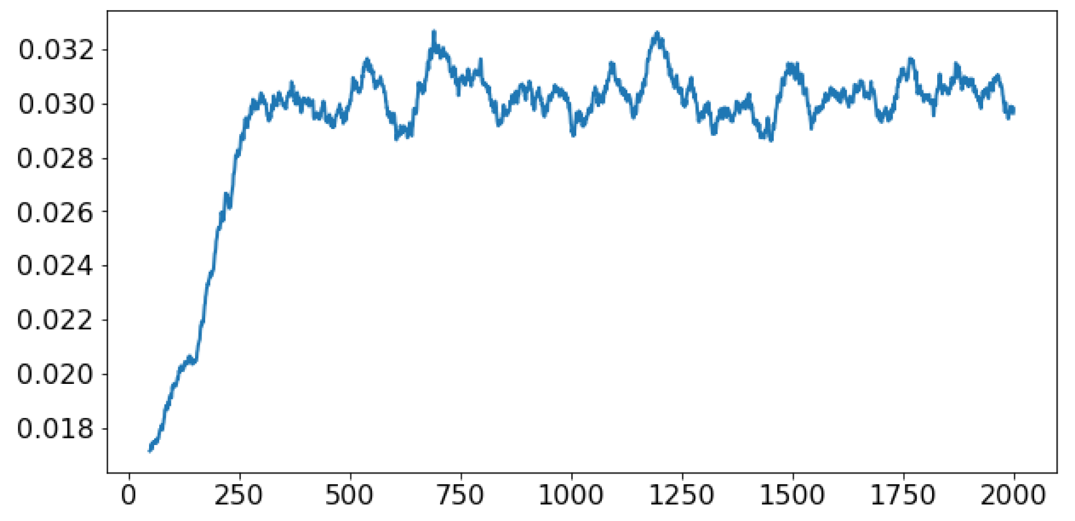
To validate our method, we consider the exponential OU process and find the value function to make a comparison with the results in [19] that uses the same model, but with a different method. Figure 3 shows how the expected payoff behaves during the training process. The x axis shows the number of epochs. As can be seen in the figure, the payoff reaches its maximum after around 250 epochs. After that point, it shows minor fluctuations, which are due to the inherent randomness in the calculation of the expected payoff.
Furthermore, as depicted in Figure 3, the learning curve stabilizes after 250 iterations, which is a sign of successful model validation in a neural network.
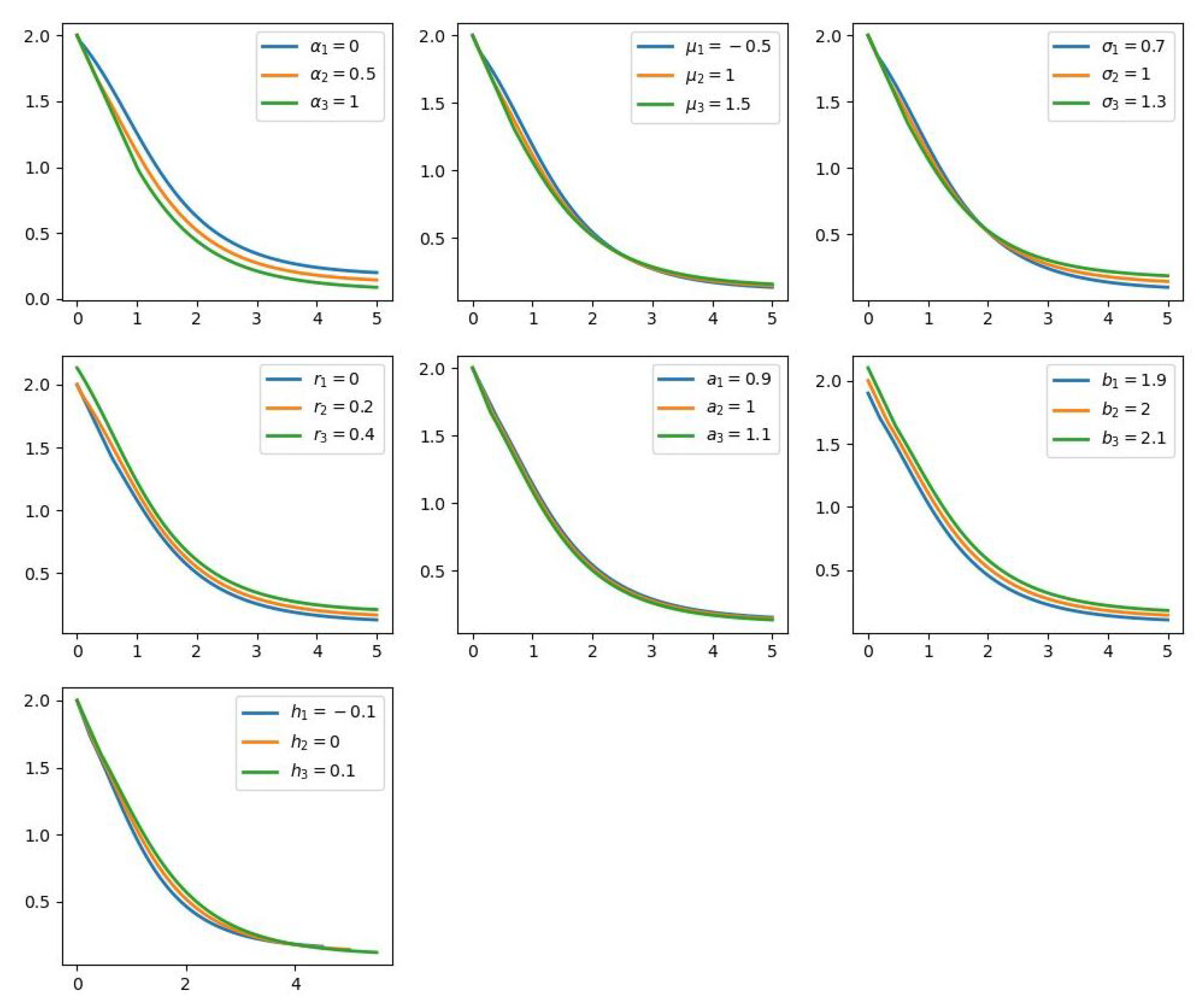
Figure 4 plots the value function for the different values of each of its parameters. The figures reveal much information about the value function. First, as can be seen, is a convex and decreasing function of x for all the illustrated values of parameters.
Second, the beginning segment of the graph of V is a linear segment. The reason for this is that for we have . This justifies our assumption that the domain D is in the form of .
Third, changing each parameter affects the value function in a monotonic way, so that V seems to be increasing with respect to and b and decreasing with respect to the remaining parameters. We will see more about the monotonicity in the sensitivity analysis section.
Comparing to the results produced in [19], the simulations match with our expectations; for instance, we see how the prices evolve with the volatility as higher volatility yields higher prices. However, we leave the interpretation of the other parameters to be read from [19]. Overall, these results show that the learning process of the neural network has generated a set of rightful value functions.
4.4. Sensitivity and Impulse Analysis
Now, let us focus on sensitivity and impulse analysis. Sensitivity analysis is essentially to see how the model reacts to changes in the model parameters, and impulse means how the model reacts to a shock to the demand. The shock to the demand is implemented by multiplying the demand process by , for a small parameter h, which represents the percentage changes in the demand.
Sensitivity and impulse analysis can be useful for a number of reasons, such as estimating how the time for the optimal storage time would delay or accelerate due to the economic shocks such as the COVID-19 catastrophe. The proposed sensitivity analysis method in this paper has applications beyond just COVID-19, as it can be used in a variety of contexts. Particularly, they can be used for calculating the Greeks of an American option or creating neutral portfolios to hedge against various risks. For example, delta hedging is a common strategy used to create a delta neutral portfolio, which is not sensitive to small changes in the underlying parameter.
4.4.1. Optimal Storage
First, let us focus on the optimal storage value . The Figure 5 and Figure 6 plot as a function of x for different values of parameters and also impulse h, for the demand process exponential OU and CIR, respectively. The confidence level is illustrated in the figures. The corresponding value of can be obtained by intersecting the confidence line with each graph.
Interestingly, the results for the two models are rather consistent, which shows the optimal storage is to a good extent to the choice of model. As one can see that the results, however, vary for different parameters. For , is decreasing, which indicates the larger mean reversion rate is one at a smaller value of the good it would decide to store. On the other hand, for , the relation is the opposite, meaning that the larger the average consumption, the larger storage value would be. Particularly, in the COVID-19 case, we can expect to see smaller for overall consumption and larger for the grocery. The behavior for is in a reverse direction than for , as more volatile demand would imply a decision for storage at a smaller value of the commodity. This is particularly important in COVID-19, as the demands for many goods have become volatile. The same is true for r and a. Note that increasing r means a higher time value, and larger a means more inelastic demand. The changes for the parameter b are not so meaningful given that we can always assume it is equal to 1. However, as one can see, the optimal value to store with respect to impulse h is increasing. This means in positive shocks there is less fear for price drops, so there is no need to rush storing goods, which makes sense.
4.4.2. Value Functions
Once the optimal decision problem has been solved, it is important to understand how the solution would react to changes in the model and impulse parameters.
One of the challenges of sensitivity and impulse analysis in the optimal stopping problem is the complex dependence of the optimal value function on the model parameters. One way to address this is to approximate the optimal value function with a simple parametric form and analyze the impulsive and sensitivity of the approximation, see [19]. However, simple parametric forms may not capture the complexity of the value function as a function of the parameters, and increasing the complexity of the parametric form can make it difficult to optimize the approximation. A network-based approach is able to capture the complexity of the value function and has well-developed optimization methods for training. This makes it a useful tool for impulse and sensitivity analysis in the optimal stopping problem.
We now focus on the exponential OU and CIR example of the previous section. We conduct a sensitivity analysis for the value function.
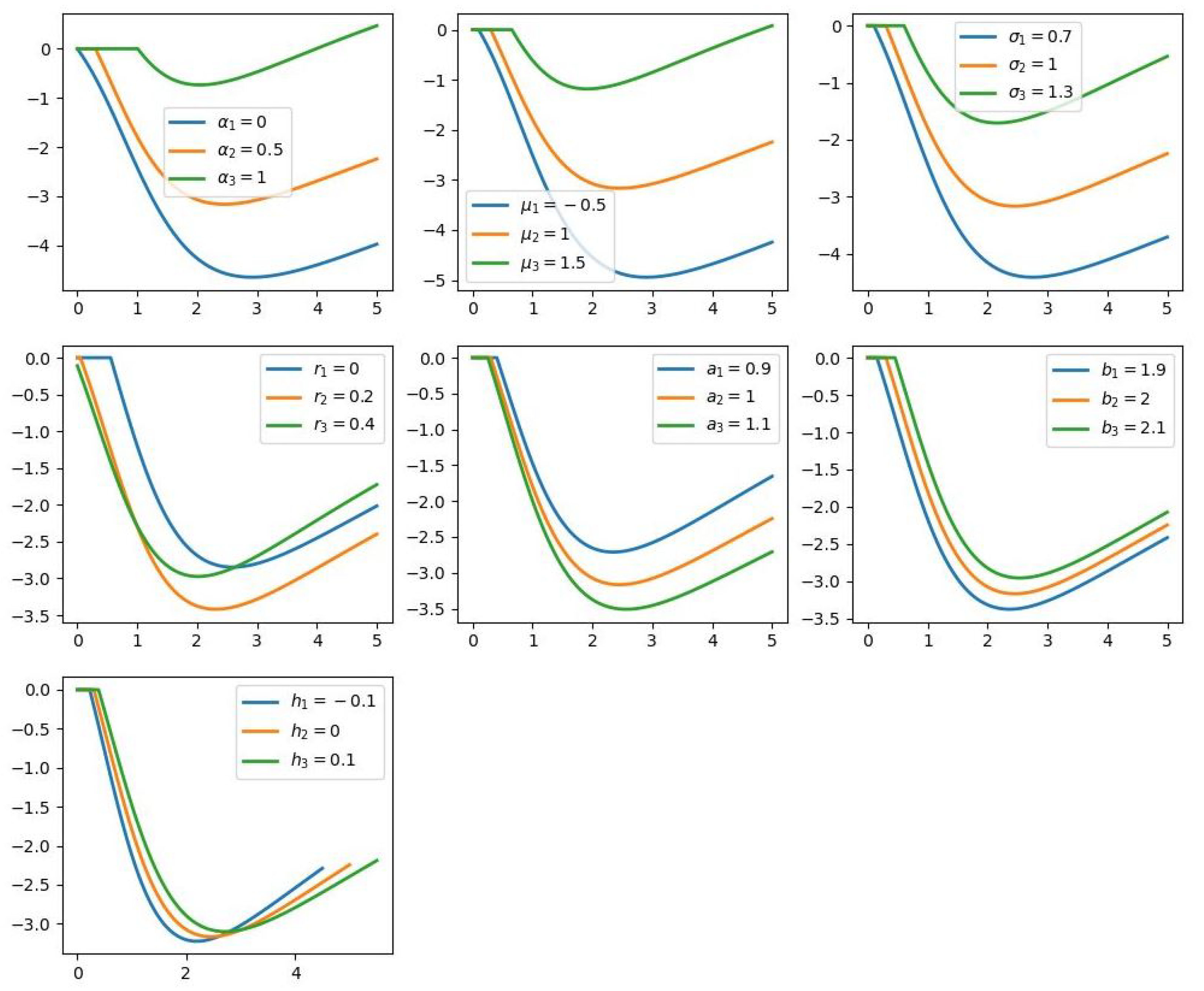
The back-propagation enables us to calculate efficiently the partial derivatives of V with respect to its parameters. This gives us a second order sensitivity analysis and illustrates the convexity and concavity with respect to each parameter. The figures of the partial derivative are shown in Figure 7 and Figure 8. As can be seen, the signs of the partial derivatives justify the monotonicity behavior that we observed in the graph of V previously.
First of all, as one can observe as with the optimal storage value, there is a consistency between the results of the two models, which makes the results very robust and reliable with respect to the changes in the modeling.
Second, the first part of all figures is constantly zero. The reason is that, for , the value function coincided with , and hence is independent of all parameters except a.
Third, as we expect, the first part of all figures are compatible with the value of that we have obtained in the previous part for optimal storage, as larger means larger values at which the figures remain equal to zero. However, in the continuation, the patterns do not always follow the same uniformity, with some figures exceeding others. Interestingly, there are values of x where in almost all figures the partial derivative reaches a minimum. This means that at a particular value, if a parameter changes, it is important whether the change is positive or negative. This means that the sensitivity of the value function to changes in the parameters and the impulse at a particular point is the smallest.
Forth, as from Figure 4, we can see that naturally if is larger, the value function itself is smaller. However, as one can see from Figure 7 and Figure 8, the opposite is true for the demand model parameters. This means at any value of the parameters, for larger x, the impact of the changes in those parameters are also larger. Interestingly, for the impulse, the behavior is changing at some point, which means while larger values for h gives larger partial derivatives with respect to h in the beginning, in one point they change the order.
As a final remark, we should mention that one can easily conduct a similar sensitivity analysis for the optimal stopping boundary, . Indeed, since each is obtained from by a simple operation, one can still use back-propagation to calculate its partial derivatives.
Remark 1.
A key benefit of our approach is that it does not depend on an analytical expression of the model and only necessitates simulated samples from the model. As a result, it can be utilized even in jump-diffusion models, although validation must be conducted for this new model. In other words, our approach is model-free.
5. Concluding Remarks
This paper presents a new method for the optimal stopping problem using artificial neural networks, that can be applied to situations where demand is shocked such as during the COVID-19 pandemic. As previously mentioned, the COVID-19 pandemic resulted in a substantial shock to the demand for certain goods, particularly food. This underscores the need for robust methods to analyze the implications of such shocks in existing economic and financial models. In this article, we concentrated on examining the impact of a shock on the price of a storable commodity. When agents are permitted to store the commodity for potential future sales, they must solve an optimal stopping problem. Thus, the value of the commodity is derived from the optimal value function. One advantage of this approach is its ability to efficiently conduct a sensitivity analysis. The method is demonstrated through two different models for commodity demand processes, where the value function and optimal stopping boundaries are calculated and sensitivity analysis is performed on all parameters, including volatility and interest rate. We obtain very robust results even after we change the models. While the optimal storage value is very consistent over all different changes, the changes to value function have different behaviors, which makes interpretation much harder. However, the results are very useful for the quantitative analysis due to robustness. The proposed method has potential applications in a wide range of optimal stopping problems in various fields, including finance.
Let us discuss some limitations and future directions of this study. A technical constraint is that, although the method is model-free, the convergence of the learning curve may depend on the nature of the process. In our case, both models, the exponential OU and CIR, are mean-reverting to a good extent, which aids in achieving convergence. However, if we were to use Geometric Brownian Motions, which are not mean-reverting, we cannot ensure that convergence will occur in a finite amount of time.
Another limitation is that the storage model considered in this study does not apply to all commodities. In particular, precious metals do not follow the same storage rules, and the model works best for agricultural goods.
There are also several interesting extensions of this model to consider in future studies. One can address the issues mentioned above, and additionally, observe the model’s performance on real data. This is a crucial task that requires a separate study, such as the one in [19], which illustrates the difficulties that arise when dealing with real data. Another future direction is to use the same methodology for non-commodity assets, such as using our method to determine the Greeks of American options.
Author Contributions
Writing—original draft, N.K., E.S. and H.A. (Hirbod Assa); Supervision, H.A. (Hojatollah Adibi). All authors have read and agreed to the published version of the manuscript.
Funding
This research received no external funding.
Data Availability Statement
No new data were created or analyzed in this study. Data sharing is not applicable to this article.
Conflicts of Interest
The authors declare no conflict of interest.
References
- Başaran, B.; Pekmezci Purut, H. The impact of the COVID-19 pandemic on the frequency of food consumption. J. Tour. Gastron. Stud. 2021, 9, 47–66. [Google Scholar] [CrossRef]
- Coulthard, H.; Sharps, M.; Cunliffe, L.; van den Tol, A. Eating in the lockdown during the COVID 19 pandemic; Self-reported changes in eating behaviour, and associations with BMI, eating style, coping and health anxiety. Appetite 2021, 161, 105082. [Google Scholar] [CrossRef]
- Fiorella, K.J.; Bageant, E.R.; Mojica, L.; Obuya, J.A.; Ochieng, J.; Olela, P.; Otuo, P.W.; Onyango, H.O.; Aura, C.M.; Okronipa, H. Small-scale fishing households facing COVID-19: The case of Lake Victoria, Kenya. Fish. Res. 2021, 237, 105856. [Google Scholar] [CrossRef]
- Pabst, A.; Bollen, Z.; Creupelandt, C.; Fontesse, S.; Orban, T.; de Duve, M.; Pinon, N.; Maurage, P. Alcohol consumption changes during the first COVID-19 lockdown: An online population survey in a convenience sample of French-speaking Belgian residents. Psychiatry Res. 2021, 300, 113938. [Google Scholar] [CrossRef]
- Güngör, B.O.; Ertuğrul, H.M.; Soytaş, U. Impact of COVID-19 outbreak on Turkish gasoline consumption. Technol. Forecast. Soc. Chang. 2021, 166, 120637. [Google Scholar] [CrossRef]
- Xiong, J.; Tang, Z.; Zhu, Y.; Xu, K.; Yin, Y.; Xi, Y. Change of Consumption Behaviours in the Pandemic of COVID-19: Examining Residents’ Consumption Expenditure and Driving Determinants. Int. J. Environ. Res. Public Health 2021, 18, 9209. [Google Scholar] [CrossRef]
- Gustafson, R.L. Implications of recent research on optimal storage rules. J. Farm Econ. 1958, 40, 290–300. [Google Scholar] [CrossRef] [Green Version]
- Muth, J.F. Rational expectations and the theory of price movements. Econometrica 1961, 29, 315–335. [Google Scholar] [CrossRef] [Green Version]
- Samuelson, P.A. Stochastic Speculative Price. Proc. Natl. Acad. Sci. USA 1971, 68, 335–337. [Google Scholar] [CrossRef] [Green Version]
- Deaton, A.; Laroque, G. On the behaviour of commodity prices. Rev. Econ. Stud. 1992, 59, 1–23. [Google Scholar] [CrossRef] [Green Version]
- Deaton, A.; Laroque, G. Estimating a nonlinear rational expectations commodity price model with unobservable state variables. J. Appl. Econom. 1995, 10, 9–40. [Google Scholar] [CrossRef]
- Deaton, A.; Laroque, G. Competitive storage and commodity price dynamics. J. Political Econ. 1996, 104, 896–923. [Google Scholar] [CrossRef] [Green Version]
- Chambers, M.J.; Bailey, R.E. A theory of commodity price fluctuations. J. Political Econ. 2001, 104, 924–957. [Google Scholar] [CrossRef]
- Ng, S.; Ruge-Murcia, F.J. Explaining the persistence of commodity prices. Comput. Econ. 2000, 16, 149–171. [Google Scholar] [CrossRef]
- Cafiero, C.; Bobenrieth, E.S.; Bobenrieth, J.R.; Wright, B. The empirical relevance of the competitive storage model. J. Econom. 2011, 162, 44–54. [Google Scholar] [CrossRef] [Green Version]
- Miao, Y.W.W.; Funke, N. Reviving the Competitive Storage Model; A Holistic Approach to Food Commodity Prices; IMF Working Paper; International Monetary Fund: Washington, DC, USA, 2011. [Google Scholar]
- Arseneau, D.; Leduc, S. Commodity price movements in a general equilibrium model of storage. IMF Econ. Rev. 2012, 61, 199–224. [Google Scholar] [CrossRef]
- Assa, H. A financial engineering approach to pricing agricultural insurances. Agric. Financ. Rev. 2015, 75, 63–76. [Google Scholar] [CrossRef]
- Karimi, N.; Assa, H.; Salavati, E.; Adibi, H. Calibration of Storage Model by Multi-Stage Statistical and Machine Learning Methods. Comput. Econ. 2022, 1–19. [Google Scholar] [CrossRef]
- Becker, S.; Cheridito, P.; Jentzen, A. Deep optimal stopping. J. Mach. Learn. Res. 2019, 20, 74. [Google Scholar]
- Becker, S.; Cheridito, P.; Jentzen, A. Pricing and hedging American-style options with deep learning. J. Risk Financ. Manag. 2020, 13, 158. [Google Scholar] [CrossRef]
- Burlacu, C.M.; Burlacu, A.C.; Praisler, M. Sensitivity Analysis of Artificial Neural Networks Identifying JWH Synthetic Cannabinoids Built with Alternative Training Strategies and Methods. Inventions 2022, 7, 82. [Google Scholar] [CrossRef]
- Guerra, M.; Nunes, C.; Oliveira, C. The optimal stopping problem revisited. Stat. Pap. 2021, 62, 137–169. [Google Scholar] [CrossRef]
- Jelito, D.; Pitera, M.; Stettner, Ł. Risk sensitive optimal stopping. Stoch. Process. Their Appl. 2021, 136, 125–144. [Google Scholar] [CrossRef]
- Herrera, C.; Krach, F.; Ruyssen, P.; Teichmann, J. Optimal stopping via randomized neural networks. arXiv 2021, arXiv:2104.13669. [Google Scholar]
- Becker, S.; Cheridito, P.; Jentzen, A.; Welti, T. Solving high-dimensional optimal stopping problems using deep learning. Eur. J. Appl. Math. 2021, 32, 470–514. [Google Scholar] [CrossRef]
- Kingma, D.P.; Ba, J. Adam: A method for stochastic optimization. arXiv 2014, arXiv:1412.6980. [Google Scholar]
- Glorot, X.; Bengio, Y. Understanding the difficulty of training deep feedforward neural networks. In Proceedings of the Thirteenth International Conference on Artificial Intelligence and Statistics. JMLR Workshop and Conference Proceedings, Sardinia, Italy, 13–15 May 2010; pp. 249–256. [Google Scholar]
- Kloeden, P.E.; Pearson, R.A. The numerical solution of stochastic differential equations. J. Aust. Math. Soc. Ser. B Appl. Math. 1977, 20, 8–12. [Google Scholar] [CrossRef] [Green Version]
- Schwartz, E.S. The stochastic behavior of commodity prices: Implications for valuation and hedging. J. Financ. 1997, 52, 923–973. [Google Scholar] [CrossRef]
- Lamberton, D.; Lapeyre, B. Introduction to Stochastic Calculus Applied to Finance; CRC Press: Boca Raton, FL, USA, 2011. [Google Scholar]
Figure 1.
Three hidden layer neural network for computation of .

Figure 2.
The USA consumption over the past two years.

Figure 3.
The expected payoff as a function of the number of epochs, evaluated for the parameters and .
Figure 3.
The expected payoff as a function of the number of epochs, evaluated for the parameters and .

Figure 4.
Each figure shows the graph of for three different values of the indicated parameter. The fixed parameters in each graph are chosen as .
Figure 4.
Each figure shows the graph of for three different values of the indicated parameter. The fixed parameters in each graph are chosen as .

Figure 5.
The figures show the graph of for three different values of each parameter indicated in the figures for the exponential OU model. The horizontal line cuts the probability of stop at a confidence level of 95%.
Figure 5.
The figures show the graph of for three different values of each parameter indicated in the figures for the exponential OU model. The horizontal line cuts the probability of stop at a confidence level of 95%.

Figure 6.
The figures show the graph of for three different values of each parameter indicated in the figures for the CIR model. The horizontal line cuts the probability of stop at a confidence level of 95%.
Figure 6.
The figures show the graph of for three different values of each parameter indicated in the figures for the CIR model. The horizontal line cuts the probability of stop at a confidence level of 95%.

Figure 7.
Sensitivity and impulse analysis of the value function of the exponential OU model. Each figure shows the graph of the partial derivative of with respect to one of its parameters, for three different values of the parameter. The fixed parameters in each graph are chosen as .
Figure 7.
Sensitivity and impulse analysis of the value function of the exponential OU model. Each figure shows the graph of the partial derivative of with respect to one of its parameters, for three different values of the parameter. The fixed parameters in each graph are chosen as .

Figure 8.
Sensitivity and impulse analysis of the value function of the CIR model. Each figure shows the graph of the partial derivative of with respect to one of its parameters, for three different values of the parameter. The fixed parameters in each graph are chosen as .
Figure 8.
Sensitivity and impulse analysis of the value function of the CIR model. Each figure shows the graph of the partial derivative of with respect to one of its parameters, for three different values of the parameter. The fixed parameters in each graph are chosen as .

Disclaimer/Publisher’s Note: The statements, opinions and data contained in all publications are solely those of the individual author(s) and contributor(s) and not of MDPI and/or the editor(s). MDPI and/or the editor(s) disclaim responsibility for any injury to people or property resulting from any ideas, methods, instructions or products referred to in the content. |
© 2023 by the authors. Licensee MDPI, Basel, Switzerland. This article is an open access article distributed under the terms and conditions of the Creative Commons Attribution (CC BY) license (https://creativecommons.org/licenses/by/4.0/).
Share and Cite
MDPI and ACS Style
Karimi, N.; Salavati, E.; Assa, H.; Adibi, H. Sensitivity Analysis of Optimal Commodity Decision Making with Neural Networks: A Case for COVID-19. Mathematics 2023, 11, 1202. https://0-doi-org.brum.beds.ac.uk/10.3390/math11051202
AMA Style
Karimi N, Salavati E, Assa H, Adibi H. Sensitivity Analysis of Optimal Commodity Decision Making with Neural Networks: A Case for COVID-19. Mathematics. 2023; 11(5):1202. https://0-doi-org.brum.beds.ac.uk/10.3390/math11051202
Chicago/Turabian StyleKarimi, Nader, Erfan Salavati, Hirbod Assa, and Hojatollah Adibi. 2023. "Sensitivity Analysis of Optimal Commodity Decision Making with Neural Networks: A Case for COVID-19" Mathematics 11, no. 5: 1202. https://0-doi-org.brum.beds.ac.uk/10.3390/math11051202
Note that from the first issue of 2016, this journal uses article numbers instead of page numbers. See further details here.