Article

An Improved Fick’s Law Algorithm Based on Dynamic Lens-Imaging Learning Strategy for Planning a Hybrid Wind/Battery Energy System in Distribution Network

1
Department of Electrical Engineering, College of Engineering, Jouf University, Sakaka 72388, Saudi Arabia
2
Department of Electrical Engineering, College of Engineering, Northern Border University, Ar’Ar 73222, Saudi Arabia
3
Department of Computer Engineering and Networks, College of Computer and Information Sciences, Jouf University, Sakaka 72388, Saudi Arabia
4
Centre for Smart Systems, AI and Cybersecurity, Staffordshire University, Stoke-on-Trent ST4 2DE, UK
*
Author to whom correspondence should be addressed.
Submission received: 30 January 2023 / Revised: 22 February 2023 / Accepted: 28 February 2023 / Published: 6 March 2023

Abstract

:
In this paper, optimal and multi-objective planning of a hybrid energy system (HES) with wind turbine and battery storage (WT/Battery) has been proposed to drop power loss, smooth voltage profile, enhance customers reliability, as well as minimize the net present cost of the hybrid system plus the battery degradation cost (BDC). Decision variables include the installation site of the hybrid system and size of the wind farm and battery storage. These variables are found with the help of a novel metaheuristic approach called improved Fick’s law algorithm (IFLA). To enhance the exploration performance and avoid the early incomplete convergence of the conventional Fick’s law (FLA) algorithm, a dynamic lens-imaging learning strategy (DLILS) based on opposition learning has been adopted. The planning problem has been implemented in two approaches without and considering BDC to analyze its impact on the reserve power level and the amount and quality of power loss, voltage profile, and reliability. A 33-bus distribution system has also been employed to validate the capability and efficiency of the suggested method. Simulation results have shown that the multi-objective planning of the hybrid WT/Battery energy system improves voltage and reliability and decreases power loss by managing the reserve power based on charging and discharging battery units and creating electrical planning with optimal power injection into the network. The results of simulations and evaluation of statistic analysis indicate the superiority of the IFLA in achieving the optimal solution with faster convergence than conventional FLA, particle swarm optimization (PSO), manta ray foraging optimizer (MRFO), and bat algorithm (BA). It has been observed that the proposed methodology based on IFLA in different approaches has obtained lower power loss and more desirable voltage profile and reliability than its counterparts. Simulation reports demonstrate that by considering BDC, the values of losses and voltage deviations are increased by 2.82% and 1.34%, respectively, and the reliability of network customers is weakened by 5.59% in comparison with a case in which this cost is neglected. Therefore, taking into account this parameter in the objective function can lead to the correct and real calculation of the improvement rate of each of the objectives, especially the improvement of the reliability level, as well as making the correct decisions of network planners based on these findings.

1. Introduction

Among renewable energies, the wind energy system is presumed amongst the most economical methods for electricity production, which is non-polluting and inexhaustible. Additionally, wind energy, like other renewable energy sources (RES), is geographically wide and at the same time scattered, almost always available. In addition, in recent years, environmental problems and issues related to climate change on the planet because of exploitation of fossil fuel-based power sources have increased the intensity of these tendencies [1,2]. Wind power can be conceived of as a source of clean and free energy. HES are used separately from the grid to supply loads far from the grid as well as sensitive loads. HES with storage devices such as batteries usually have higher reliability, as well as lower electricity generation costs, than individual systems. The presence of storage systems within power systems is necessary due to the random nature of wind energy [3,4]. Energy reliability under different weather conditions and related costs are two important issues when designing renewable energy systems. To make an energy system economical, the optimal design of these types of systems is necessary so that the optimal size of the devices to supply a specific load is obtained [5].
Furthermore, the interconnection of HES and large-scale power systems helps exchange power [5]. To achieve maximum benefits from renewable energy systems across distribution networks, the optimal site and size of these systems in the power system should be optimally determined. In recent years, distribution network operators have paid much attention to the scheduling of HES in electricity distribution networks. Hybrid wind energy systems integrated with battery storage are one of the most popular systems to enhance the features of electricity distribution networks by creating electrical scheduling with optimal power injection into the network. On the other hand, the capacity of batteries is reduced by charging and discharging energy, and thus, this problem is a major challenge for high-capacity applications. Battery degradation is caused by storage cycles as well as the charging and discharging process, which is created slowly. Battery degradation is measured based on two indices: calendar life and cycling life. The calendar indicates the expected number of years of battery life, while the latter represents the expected number of charge–discharge cycles of the battery before entering the resistance increase threshold mode. Therefore, considering battery degradation as an effective factor in scheduling HES based on battery storage should be considered and its effect on improving the distribution system’s indices should be assessed. In scheduling HES in distribution systems, their optimal installation location and power distribution of RES, besides the charge–discharge pattern of the storage units, should be optimally determined, and this optimization is performed using intelligent meta-heuristic methods in a facilitated and correct form [5,6].
The following presents a summary of studies conducted in the field of designing HES and the placement and planning of distributed power sources within distribution networks, especially by focusing on RES-dependent energy systems. In [7], the design of a RES with wind and solar-based power sources and also battery storage for Nepal is presented and the cost imposed on producing power is minimized. Ref. [8] designs a HES by adopting a linear programming method with the purpose of minimization of the investment and maintenance cost to supply the annual load. In [9], a grid-connected HES is optimally designed and developed based on multi-objective optimization with a fuzzy logic method and optimal ratings of the load-supplying equipment are obtained. Genetic algorithm (GA) was adopted [10] to discover the proper capacity of a wind–photovoltaic system by minimizing the investment cost and limiting the reliability. Ref. [11] models a wind–photovoltaic energy system for reliable supply of an annual load is presented to minimize the energy cost using GA and PSO algorithms. Ref. [12] optimally sizes a photovoltaic–wind–battery system by employing the fuzzy adaptive GA via determining the optimization variables. In [13], the optimal planning of an islanded energy system that feeds thermal and electrical load of a residential complex has been implemented using the binary GA. In [11], a grid-disconnected photovoltaic–wind energy system has been designed so that electrical demand of a load is met, and cost imposed by producing electrical power is minimized with the help of an improved PSO. The literature [14] presents a procedure using the PSO to achieve appropriate scale of an islanded photovoltaic–wind system that contains hydrogen storage and to meet the reliability constraint. Ref. [15] determines the components capacity of a wind–photovoltaic energy system to make energy cost as small as possible through the modified PSO. The authors in [16] optimally designed a wind–photovoltaic energy system with a battery bank so that the system cost is minimized by adopting multi-objective PSO (MOPSO). In [17], a wind–photovoltaic–fuel cell energy system is optimally scaled using the PSO and the minimum overall energy cost is found considering the equivalent loss factor (ELF). In [18], the cost-effective layout of an islanded wind–photovoltaic energy system in Mexico has been developed to minimize the overall system cost of supplying the annual load by using PSO. In [19], the optimal design of a HES that consists of photovoltaic, wind, and battery storage was developed to make the energy cost minimized using the spider community optimization algorithm (SSO) for Saudi Arabia. Ref. [20] achieves the size of a photovoltaic–wind energy system containing a battery bank and diesel support that feeds the annual load so that the minimum lifetime cost is achieved by incorporating nomadic people optimization (NPO) in Iraq. In the following, some of the research concerning the optimal siting of RES in distribution systems as well as the planning of HES are presented for radially structured distribution systems. Ref. [21] focuses on finding the optimal place of photovoltaic and wind systems in radial distribution systems by taking into account power loss on the distribution lines and reliability index using the flame propeller optimization (MFO). In [22], the same purposes of [21] are followed but aiming to minimize power loss and enhance network reliability by incorporating a hybrid learning–gray wolf algorithm (MOHTLBOGWO). In [23], the problem of finding the place and scale of wind turbines is formulated in the form of a single objective in the radial distribution system to minimize the loss using the GA. In [24], the PSO is applied for siting photovoltaic sources in an unbalanced distribution system so that the voltage profile becomes smoother and power loss is minimized. The literature [25] allocates a photovoltaic and wind turbine system to decrease power loss and voltage variation by adopting PSO. In [26], a two-stage optimal allocation method based on the PSO has been developed for photovoltaic systems to minimize power loss. In [25], the optimal place and size of photovoltaic and wind systems has been found to reduce power loss as much as possible and stabilize voltage with the help of the PSO. Ref. [27] discusses the optimal siting of photovoltaic and wind sources in a distribution system via the ALO to drop power loss, enhance voltage profile, and consequently stabilize the voltage. The paper used a multi-objective approach relying on weighting coefficients. In [28], the sizing of a HES including wind and photovoltaic sources besides battery banks is developed to minimize energy and emission costs using the spotted hyena optimization (SHO). In [29], the optimal layout and multi-objective allocation of a hybrid system with photovoltaic, wind turbines, and battery storage is implemented in a radial distribution system to diminish power loss, smooth voltage profile, and decrease energy production costs using weight coefficients method and improved whale optimization method (IWOA). Ref. [30] finds the optimal capacity and place of a hybrid wind–photovoltaic system containing battery units to make power loss and voltage variation as small as possible by incorporating an improved crow search algorithm (ICSA).
The contributions of the paper are described based on the research gaps in the literature as follows:
  • Most studies on HES suppose them in grid-disconnected form and focus on the sizing methods. Few studies have addressed the planning of HES with battery units in distribution networks, in which reliability studies have not been presented well.
  • In the HES, the storage unit compensates for power fluctuations of RES and improves reliability. Battery degradation assessment is presented as a crucial factor when designing off-grid HES. However, as far as the authors know, the effect of BDC on planning of HES in the radial distribution system and its effect on the improvement of network characteristics considering reliability has not been addressed.
  • A fast solver needs to be adopted to deal with optimization problems. Based on the NFL theory, a meta-heuristic method may show a good ability to achieve the global optimum in solving many optimization problems, even though it might fail to achieve the optimal solution of some problems. Thus, the motivation behind using novel metaheuristic methods to address planning problems of HES in distribution systems is to discover the installation points and optimal power flow of the HES.
The planning scheme of the WT/Battery system is proposed in the current study by expressing it as a multi-optimization problem. It is solved to minimize power loss, smooth voltage profile, improve reliability, as well as minimize the present cost and BDC. Providing a metaheuristic algorithm with powerful exploration and exploitation capabilities to prevent premature convergence can determine the optimal site and size of hybrid system components in a distribution system so that the maximum improvement of planning objectives is achieved. Therefore, there is still a need for an optimal and multi-objective planning framework for the HES with energy storage devices in the distribution system by employing a metaheuristic algorithm with the optimal ability to scape local minima/maxima. The present work improves the performance of the Fick’s law algorithm (FLA) [31] to enhance the exploration performance and prevent premature convergence based on the dynamic lens-imaging learning strategy (DLILS) based on improved opposition learning and the improved FLA algorithm (IFLA) is formed. The suggested approach is implemented on a 33-bus distribution system and the simulation results which include power losses, network voltage profile, and reliability in the form of energy not supplied are compared before and after planning. Additionally, the impact of BDC on individual objectives is investigated. Moreover, a comparison is made between the performance of the IFLA and FLA, PSO, MRFO, and BA when applied to solve the planning problem.
Important remarks and achievements of the present work are highlighted here:
  • Optimal multi-objective planning of a hybrid WT/Battery energy system in a distribution system.
  • Providing a multi-objective function considering power loss, voltage profile, reliability, net present cost, and storage degradation cost.
  • Evaluation of the effect of BDC on the multi-objective planning problem.
  • Using an improved Fick’s law algorithm based on a dynamic lens-imaging learning strategy.
  • Superiority of the suggested IFLA-based method to the FLA, PSO, MRFO, and BA.
Section 2 models the hybrid WT/Battery energy system. Section 3 formulates the proposed problem including the objective function and constraints. The proposed meta-heuristic algorithm and its use in solving the planning problem are given in Section 4. Eventually, Section 5 provides the results obtained from simulations and gives a discussion on the results, and Section 6 presents the conclusions.

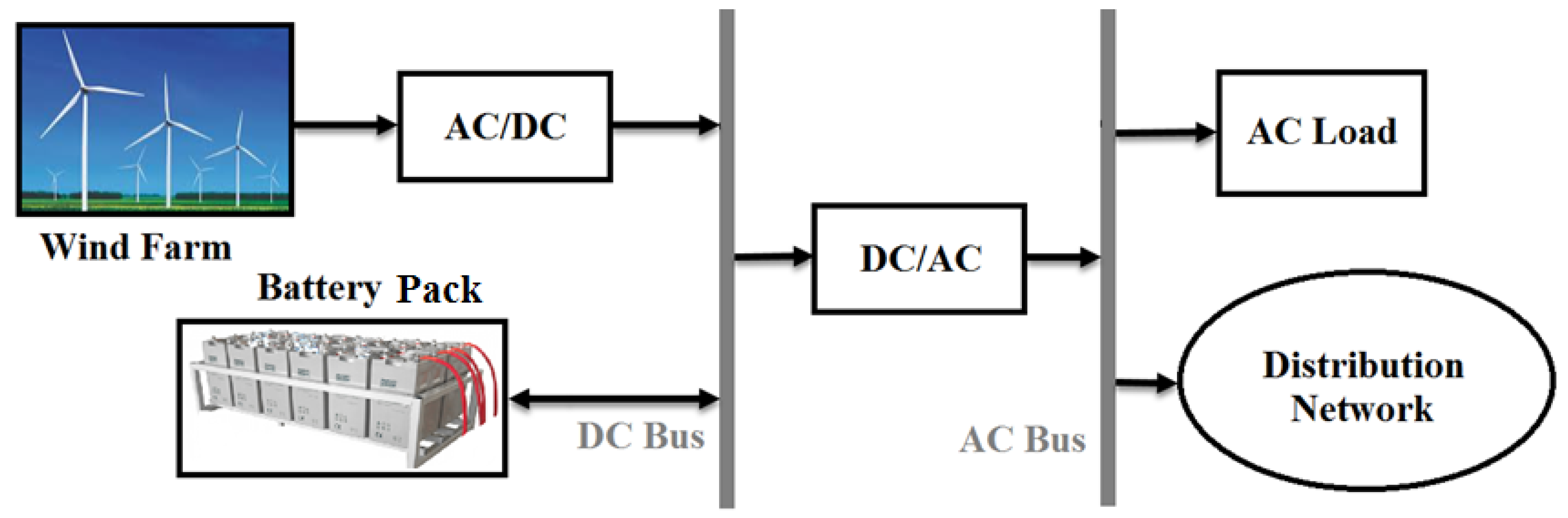
2. Hybrid WT/Battery Energy System

2.1. Operating Conditions

Planning of a hybrid WT/Battery system according to Figure 1 has been performed in the distribution network. In the case the power generation by the wind farm becomes greater than the amount of the demand, then it is assumed that 50% of the excess power over the demand of the hybrid system is injected to charge storage units (batteries) and the other 50% will be fed into the distribution system. In this condition, the batteries are in charging mode. On the other side, when there is shortage in the power output of the wind farm, the power required by the hybrid system load is met via battery discharging. The role of battery storage is to reduce power variations of the wind farm and inject programmable power of the HES into the distribution system. The demand is assumed to be fully met by the proposed HES.

2.2. Modeling of the HES

2.2.1. Wind Generator Power Model

The power generation ( p W G ) by a wind turbine has a nonlinear relationship with cut-in, rated, and cut-off wind speeds, as given by Equation (1) [5,12].
p W G = 0 ;                                                                                           W S W S c i n , W S W S c o u t p W G N o m × W S W S c i n W S n o m W S c i n ; W S c i n W S W S n o m p W G N o m ;                                                               W S n o m W S W S c o u t
where W S indicates the wind speed and W S c i n , W S c o u t , and W S n o m indicate the cut-in, cut-out, and nominal speeds, respectively. p W G N o m is the nominal power output.
Considering Equation (1) and the possible exit of wind sources based on reliability concepts, P W G considering the maximum number of wind generators W G f a i l and failed generators ( W G f a i l ) is defined as follows:
P W G = W G W G f a i l × p W G

2.2.2. Modeling the Battery Storage

In the HES, batteries are used to compensate for power fluctuations of energy sources. The operation of the battery storage system depends on their charging and discharging patterns [5,12,19]. In the following, the operation of the storage system is presented according to charging and discharging strategies.
  • Charging strategy: In this strategy, in the case the production power by wind generators exceeds the demand of the HES, it is assumed that 50% of the excess power over the demand of the HES is stored in battery units and the remainder can be fed into the distribution system. The power output of a battery bank at time t can be defined as follows:
P B a t t e r y t = P B a t t e r y t 1 × 1 σ + 0.5 × P W G t P H S t η I n v × η B a t t e r y
where P B a t t e r y t and P B a t t e r y t 1 denote the battery charge at times t and t − 1, respectively. P H S t represents the required power of the HES demand at time t, σ expresses the rate of self-discharge of the battery, η I n v shows the inverter efficiency, and η B a t t e r y is the charging efficiency of the battery.
  • Discharge strategy: In discharge strategy, if the production power of the wind generators cannot meet the demand, then the battery power can be discharged so that it fully meets the demand required by the hybrid system (the demand is assumed to be fully met during the study period). The power output from the battery bank at time t will be defined in Equation (4):
P B a t t e r y t = P B a t t e r y t 1 × 1 σ P H S t η I n v P W G t / η I n v

2.3. Modeling the Hybrid System Cost

The system cost model depends on the cost imposed by components, which includes investment cost, maintenance cost, and replacement cost during the life of the hybrid system project, and it is given by Equation (5) [5,12,19]:
N P C T = N P C I + N P C M + N P C R + C B D
where N P C T represents the present value of the HES. N P C I , N P C M , and N P C R represents the costs related to investment, maintenance, and replacement of equipment, respectively.

2.3.1. Investment Cost

The investment cost including the purchase cost of wind generators, batteries, and inverter is defined as follows [5,12,19].
N P C I = C o W G , I × W G + C o B a t t e r y , I × B a t t e r y + C o I n v , I × I n v
where C o W G , I , C o B a t t e r y , I , and C o I n v , I denote the purchase of each unit of wind generator, battery, and inverter, respectively. W G , B a t t e r y , and I n v represent the number of wind generators, batteries, and inverters, respectively.

2.3.2. Maintenance Cost

The maintenance cost of HES equipment will be [5,12,19]:
N P C M = C o W G , M × W G + C o B a t t e r y , M × B a t t e r y × t = 1 T 1 + I n f R 1 + I n t R t
where C o W G , M and C o B a t t e r y , M represent the yearly maintenance cost of wind generators and batteries, respectively. In the present study, the maintenance costs of the inverter are ignored.

2.3.3. Replacement Cost

In this study, according to the lifespan of batteries and inverters, only the cost of replacing them is considered. The equipment replacement cost is defined as follows [5,12,19]:
N P C R = C R B a t t e r y , R × B a t t e r y + C R I n v , R × I n v × t = 1 T 1 + I n f R 1 + I n t R t
where C R B a t t e r y , R and C R I n v , R represent the replacement cost of each wind turbine and inverter unit, respectively. I n f R and I n t R represent the inflation rate and interest rate, and T represents the study period of 8760 h.

2.3.4. Battery Degradation Cost (BDC)

The degradation cost of the grid-connected batteries is added to the net present cost function of the system to evaluate how battery degradation impacts the total cost. According to planning the HES with battery units in a short time horizon, the cycle life is considered to measure the degradation cost. BDC is defined as follows [32,33,34]:
C B D = C o B a t t e r y × B a t t e r y × D O D × P B a t t e r y × Δ t N u C y c l e
where C o B a t t e r y represents the investment cost of the battery, P B a t t e r y represents the battery power, and Δ t is the time interval (1 h). Depth of discharge (DOD) of the battery pack is calculated as follows [32]:
D O D = P B a t t e r y , M a x P B a t t e r y , i P B a t t e r y , M a x
where P B a t t e r y , M a x represents the maximum storage power in the battery and P B a t t e r y , i refers to the storage energy in the battery in a given hour of the study horizon.
The cycle life of the battery can be expressed by Equation (11):
N u C y c l e = τ × D O D μ
where τ and μ represent the specific parameters of the battery, which are 1331 and −1.825 [32] for lithium-ion battery, respectively.

3. Problem Formulation

The problem of hybrid WT/Battery system planning is presented in the 33-bus distribution system. Thereby, the design cost ( N P C T ) is minimized, the active power loss and voltage anomalies of buses are minimized, and the reliability of subscribers is also improved. The objective function of hybrid system design cost ( N P C T ) is formulated in Section 2 by considering the BDC. Here, the multi-objective function is presented according to the method of weighting coefficients, and functions related to the network, including active power loss, voltage profile, and network reliability are formulated, and the constraints of the problem are also presented.

3.1. Objective Function

The objective function for planning the HES with battery storage in the radial distribution system is described to minimize active power loss, smooth network voltage profile, increase reliability of network subscribers, as well as minimize the components cost along with BDC:
φ O F = ξ 1 × φ 1 O F φ 1 , m a x O F + ξ 2 × φ 2 O F φ 2 , m a x O F + ξ 3 × φ 3 O F φ 3 , m a x O F + ξ 4 × φ 4 O F / φ 4 , m a x O F
where φ 1 O F , φ 2 O F , φ 3 O F , and φ 4 O F represent active power loss function, network voltage deviation function, reliability function, and NPCT cost function, respectively. φ 1 , m a x O F , φ 2 , m a x O F , φ 3 , m a x O F , and φ 4 , m a x O F , respectively, represent the maximum loss of active power loss, voltage deviation, and maximum NPCT cost budget of the hybrid system. ξ 1 , ξ 2 , ξ 3 , and ξ 4 are the weight of different terms of the objective function, where ξ 1 + ξ 2 + ξ 3 + ξ 4 = 1 . Note that the fourth objective function, i.e., φ 4 O F , is expressed in the previous section using Equations (5)–(11). Based on the trial and error method and also a fair view of all objectives, the value of each of the weight coefficients is considered to be 0.25. The rest of the objectives, i.e., power loss reduction, voltage profile, and reliability enhancement of a distribution network subscribers, are mathematically defined in the following.

3.1.1. Power Losses

Distribution system operators always seek to make the active power losses ( P L o s s ) minimized. Therefore, this is considered in the planning problem of the WT/Battery hybrid system. Active power losses are presented as follows [29,30]:
φ 1 O F = P L o s s = i = 1 N b r a n c h R i × I i 2
where P L o s s represents the loss of active power, Ri represents the resistance of line i, I i represents the current of branch i, and N b r a n c h is the number of lines.

3.1.2. Voltage Deviations

The improvement of the voltage profile can be realized by reducing voltage variations in the buses. The objective function formulated to minimize this quantity can be expressed by Equations (14) and (15) [35]:
φ 2 O F = 1 N b u s × i = 1 N b u s ( v i v p ) 2
v p = 1 N b u s × i = 1 N b u s v i
where vi represents the i-th bus voltage, vp shows the average bus voltage, and Nbus is the number of buses.

3.1.3. Reliability

Reliability can be assumed as one of the critical parameters that should be enhanced when discussing the the operation of distribution networks. In this section, the objective of minimizing the energy not supplied (ENS) of users due to the outage of the lines can be defined [2,22].
φ 3 O F = E N S N e t w o r k T = i = 1 N b r j = 1 N l R O U i × ξ i × R Τ i × I L j
where E N S N e t w o r k T represents the disconnected energy of the subscribers, N l shows number of disconnected loads, R O U i is the value of line i outage, ξ i is the length of line i, R Τ i is the repair period of line i, and I L j indicates the amount of cut-off load due to the line i outage.

3.2. Problem Constraints

The constraints of the planning problem, based on which the objective function should be bound, are presented as follows:

3.2.1. Wind Farm Power

The power generated by wind farm should be maintanied between its lower and upper bounds:
P W G M i n P W G P W G M a x
where P W G M i n and P W G M a x represents the minimum and maximum power generation by a wind farm, respectively.

3.2.2. Battery Bank Capacity

The capacity of the battery bank must be kept within the allowed range:
P B a t t e r y M i n P B a t t e r y P B a t t e r y M a x
where P B a t t e r y M i n and P B a t t e r y M a x represents the minimum and maximum power size of a battery bank, respectively. The formula will be written as:
P B a t t e r y M i n = 1 D O D × P B a t t e r y M a x
where DOD represents the maximum depth of discharge of the battery unit.

3.2.3. Voltage of the Network Buses

This cvonstraint states that the voltage magitude at each bus should be within the specified range:
V B u s M i n V B u s V B u s M a x
where V B u s M i n and V B u s M a x show the minimum and maximum magnitudes of bus voltages, respectively.

3.2.4. Maximum Permissible Line Current

The thermal limitation of grid lines is applied by the following expression:
I L i n e M i n I L i n e I L i n e M a x
where I L i n e M i n and I L i n e M a x represent the minimum and maximum allowed current flow on network lines, respectively.

3.2.5. Power Balance

The active and reactive powers should be balanced in the system as follows:
P P o s t + i = 1 N W T / B a t t e r y P W T / B a t t e r y i = i = 1 N b r a n c h P l o s s i + q = 1 N b u s P d q
Q P o s t + i = 1 N W T / B a t t e r y Q W T / B a t t e r y i = i = 1 N b r a n c h Q l o s s i + q = 1 N b u s Q d q
where P P o s t , P W T / B a t t e r y , P l o s s , and P d represent the active power received from the substation, the active power fed into the network by the HES, active losses of the line, and active power need of the network load, respectively. Q P o s t , Q W T / B a t t e r y , Q l o s s , and Q d represent the reactive power received from the substation, the reactive power fed into the network by the HES, the line reactive losses, and the reactive power needed, respectively. N W T / B a t t e r y represents the number of hybrid systems (here, 1).

4. The Suggested Optimization

The optimal design and planning of the WT/Battery system in the radial distribution system can be formulated as a nonlinear optimization problem. The present paper adopts a novel optimization method called the improved Fick’s law algorithm (IFLA) based on the DLILS to solve the planning problem.

4.1. Overview to the FLA

The Fick diffusion law has been adopted in structuring a new optimization tool and is employed in the present research to optimally plan a hybrid WT/Battery system. The FLA includes diffusion, equilibrium, and steady state phases. The FLA is a powerful optimization method that can fairly perform exploration and exploitation processes by balancing these phases [31].

4.1.1. Inspiration

The motion of particles between different concentrated points in the space follow the Fick diffusion equations. It states that “diffusion speed is directly related to surface area and concentration difference and inversely related to membrane thickness”. A diffusion based on the rules of Fick is called normal propagation or Fick. In FLA algorithm, Fick’s law is simulated so that stable positions of molecules are found. In this algorithm, three motion operators including (1) diffusion operator (DO), (2) equilibrium operator (EO), and (3) steady state operator (SSO) are provided. In the DO phase, it is assumed that there are two regions at the beginning of the experiment with considerable concentration difference, which forces the particles to move and replace other particles’ positions. In the EO phase, the two concentrations are approximately the same and the particles attempt to find an equilibrium. The SSO phase happens when particles change their positions region based on the best stable position in this region.

4.1.2. Formulation of FLA

The FLA algorithm is presented mathematically as described below.
Step 1: Initialization. In the FLA, optimization starts based on a set of candidate solutions, shown by X, according to Equation (24). The generation of solutions is random and, in each iteration, the best solution is selected as the best current almost optimal solution [31].
  x 1 , 1 x 1 , j x 1 , D x 2 , 1 x 2 , j x 2 , D x N , 1 x N , j x N , D 1 x N , D
where N represents the number of solutions (population size), D represents the dimension of the problem (number of variables), and j refers to the jth decision variable.
Step 2: Clustering. At this step, the population of the algorithm is divided into two equal groups, N1 and N2.
Step 3: Transfer function (TF). The efficiency of any algorithm is highly dependent on the transition from discovery to exploitation and vice versa. In the FLA, a nonlinear transfer function (TF) is provided for this problem. TF function is defined as Equation (25) [31].
T F t = s i n h ( t / T ) c 1
where t and T show the number of iterations and maximum number of iterations, respectively, and c 1 is considered 0.5.
Step 4: Update the molecule position. In this step, three phases based on transfer operators, namely DO, EO, and SSO, are presented. The transition process between the three phases is based on the following equation [31]:
X i t = D O T F t < 0.9 E O T F t 1 S S O T F t > 1

4.1.3. DO Operator (Discovery Phase)

If there is a high concentration difference between two regions, molecules change their position according to the region concentration. T’DO is defined as follows [31].
T D O t = C 5 × T F t r , C 5 = 2
The flow direction is determined according to the value of T’DO as follows [31]:
X p , i t = from   i   to   j   region ;   T D 0 t < r a n d from   j   to   i   region ;   otherwise
If the concentration of region i is higher than that of region j, some molecules will migrate from region i to region j, and other remaining molecules in region i are influenced by this movement. The number of molecules transferred can be defined as follows [31]:
N T i j N i × r 1 × C 4 C 3 + N i × C 3
where NTij shows how many molecules moved between group i and group j, and C3 and C4 are fixed numbers with values of 0.1 and 0.2, respectively.
The number of remaining molecules within molecular group i is determined as follows [31]:
N R i j N i N T i j
NTij means transferred molecules then move to another region and their position is mainly updated with respect to the best equilibrium molecule in region j as follows [31]:
X p , i t + 1 = X E O , j t + D F p , j t × D O F × r 2 × J i , j t × X E O , j t X p , j t + 1
where X E O , j t represents the equilibrium position in region j, and D F i t refers to the direction factor which is equal to {−1, 1} and has random changes. This factor causes a stronger search of the search space and avoids getting trapped in the local optimum. r2 is a numerical expression between the closed interval 0 and 1 randomly. Additionally, DOF indicates the time-varying flow direction, which is defined as Equation (31) [31].
D O F = e x p ( C 2 T F t r 1 ) , C 2 = 2
J i , j t refers to the diffusion flux, which is presented as follows [31]:
J i , j t = D d c i , j t d x i , j t
where D represents the effective diffusion constant and its value is considered to be 0.1, while d c i , j t / d x i , j t represents the concentration gradient and is defined based on Equations (33) and (34) [31]:
d c i , j t = X m , j t X m , i t
d x i , j t = ( x E O , j t ) 2 ( x p , i t ) 2 + e p s
where X m , j t and X m , i t refer to the average position of the molecule in regions i and j, respectively.
The positions of remaining molecules in the ith group in region i are updated based on the movement between distinct stages (equilibrium positions in regions i and j and problem boundary and no change in the positions). This strategy can be described by Equation (35) [31]:
X p , j t + 1 = X E O , i t ;   r a n d < 0.8 X E O , i t + D O F × ( r 3 × U L + L ;   r a n d < 0.9 X p , i t + 1 ;   otherwise
where X E O , i t represents the equilibrium position in region i, U and L denote the upper and lower limits of the problem, and r3 represents a random number between 0 and 1.
Molecules in region j modify their position in the same region due to its higher concentration without traveling, i.e., their position is updated relative to the equilibrium point. The problem boundary is defined by Equation (36) [31]:
X p , j t + 1 = X E O , j t + D O F × ( r 4 × U L + L )

4.1.4. EO Operator (Transition Stage from Exploration to Exploitation)

At this step, the exploration phase is transferred to exploitation. The position of molecules is updated based on Equation (37) [31].
X p , g t + 1 = X E O , p t + Q E O , g t × X p , g t + Q E O , g t × M S p , E O t × X E O , g t X p , g t
where X p , g t represents the location of particle p in the group, X E O , g t refers to the equilibrium position in group g, and Q E O , g t and M S p , E O t are defined as Equations (38) and (44) [31].
Q E O , g t = R 1 t × D F g t × D R F E O , g t
where Q E O , g t represents the relative quantity of the region in group g and D R F E O , g t represents the diffusion rate coefficient in the group, which is obtained as follows [31]:
D R F E O , g t = e x p ( J p , E O t T F t )
In (39), J p , E O t is obtained as follows [31]:
J p , E O t = D d c g , E O t d x p , E O t
where d c g , E O t and d x p , E O t are determined as follows [31]:
d c g , E O t = x g , E O t X m , g t
d x p , E O t = ( x g , E O t ) 2 ( x p , g t ) 2 + e p s
D F g t = ± 1 :   direction   factor
M S p , E O t = e x p ( F S g , E O t F S p , g t + e p s ) :   motion   step
R 1 t = r a n d [ 0 , 1 ] d ;   d = 1 : dimension
where F S g , E O t represents the best fitness value in group g at time t and F S i , g t denotes the particle fitness value in group p at time t.

4.1.5. Steady State Operator (SSO) (Exploitation Phase)

The exploitation phase is the final step in the optimization problem. In this step, the position of the molecules will be updated based on the following equation [31]:
X p , g t + 1 = X s s t + Q g t × X p , g t + Q g t × M S p , g t × X s s t X p , g t
where X s s t and X p , g t represent the location of the steady state and the position of the p particle, respectively. Additionally, Q g t and M S p , E O t expresses the relative quantity of the g region and refers to the transition step, which are determined based on Equations (28) and (30) [31].
Q g t = R 1 t × D F g t × D R F g t
In (47), D F p t represents the direction factor equal to ±1, R 1 t varies between [0, 1] randomly, and D R F p t expresses the signal diffusion speed factor, which is obtained as follows [31]:
D R F g t = e x p ( J p , s s t T F t )
M S p , g t = e x p ( F S s s t F S p , g t + e p s )
J p , s s t is determined as follows [31]:
J p , s s t = d c g , s s t d x p , s s t
where d c g , s s t and d x p , s s t are calculated based on the following equations [31]:
d c g , s s t = x m , g t X s s t d x p , s s t = ( x s s t ) 2 ( x p , g t ) 2 + e p s

4.1.6. Balancing the Exploration and Exploitation Phases

Establishing a balance between exploration and exploitation phases is essential when dealing with optimization algorithms. The FLA consists of diffusion, equilibrium, and steady state steps. Exploration is based on a simulated diffusion phase, by which molecules discover the entire search domain. Then, the transition between exploration and exploitation can be implemented based on the equilibrium stage. Finally, following the steady state stage, the exploitation of molecules from promising areas is established.
According to the explanations, Algorithm A1 shows the step-by-step process of the FLA (see Appendix A).

4.2. Overview of the IFLA

In solving some optimization problems, optimization algorithms may experience an iterative stagnation, slow convergence, or premature convergence. In this situation, exploration and exploitation phases in solving such problems are more important. Here, the strategy to improve the efficiency of FLA is presented and explained. The DLILS is a learning method based on opposition learning [36]. In Figure 2, the DLILS is depicted. There is an individual F (molecule) on the left of axis y, and its projection on axis x represents X and its distance from axis x represents ξ . Axis y is a convex lens with a focal length of f, whose center is point O. When F flows through a convex lens, an opposing F’ is created and its image created on the x-axis is equal to X’ and its distance from axis x is indicated by ξ . Person X and opposite person X’ have been created.
As per Figure 2, X and X′ are calculated using the convex lens imaging principle:
ψ u + ψ l 2 X X ψ u + ψ l 2 = ξ ξ
where ψ u and ψ l show the upper and lower limits. Suppose ξ / ξ = μ   and μ represents the scaling factor. Equation (52) is rewritten and solved for X′:
X = ψ u + ψ l 2 + ψ u + ψ l 2 × μ X μ
The scalability factor μ can empower the local development potential of FLA. In DLILS, scaling factors are chosen as fixed, which weakens the algorithm’s convergence capability. A scaling factor with nonlinear dynamic reduction is presented so that the diversity of the algorithm is improved by increasing the search capability of the algorithm in a wider range. Therefore, based on this search near the optimal particle, the local search potential is strengthened and prevents getting trapped in the local optimum. The nonlinear dynamic scaling factor α is defined as follows:
μ = λ m i n λ m a x λ m i n × t T 2
where λ m a x shows the maximum scaling factor, λ m i n denotes minimum scaling factor, and T represents the maximum repetitions. λ m a x and λ m i n are considered 100 and 10. Equation (53) in the n-dimensional search space will be given as follows [36]:
X j = ψ u j + ψ l j 2 + ψ u j + ψ l j 2 × α X j α
where X j and Xj denote, respectively, the components of X0 and X in dimension j and ψ l j and ψ u j show the lower and upper limits of dimension j, respectively. The DLILS determines the best solution by fitness evaluation, considering candidate and opposing solutions.
The opposition-based learning (OBL) strategy has a form of Equation (53) with μ = 1 . The OBL strategy can be used to boost the overall exploration in the initial steps [36] and has the ability to diversify the population. However, by continuation of the iterations, the algorithm goes from global optima to local optima. To solve this issue, DLILS has been used.

4.3. Evaluating the Performance of the IFDA to Solve Test Functions

The performance of IFLA when used for solving classical test functions, including unimodal, multimodal, and fixed-dimensional polynomial functions, is discussed here [37]. The suitable performance of IFLA than that of conventional PSO, MRFO, and FLA algorithms is investigated. Table 1 reports the parameters used in optimization algorithms. As is observed, the IFLA has reached the optimal solution with better convergence capability and stronger competition compared to other algorithms with better values of statistical indices. Table 2 lists the reports related to the algorithms. In Table 2, symbols “+”, “−”, and “≈” show the performance of competitor is significantly better than, worse than, and almost similar to that of the IFLA, respectively. As one can observe, the IFLA provides more desirable results than its counterparts. Furthermore, the results of the Wilcoxon test [37] can be seen in Table 3, which confirmed that the proposed algorithm decisively wins over all algorithms and has better convergence efficiency.

4.4. The IFLA Implementation

The IFLA is implemented to solve the planning problem of the WT/Battery system in the distribution network.
  • Step (1) Initiate data. The data related to the load in active and reactive network along with R and X data of distribution network lines, the data of the system components, including wind speed data and components cost specifications, population number, and maximum iteration of IFLA are used as inputs.
  • Step (2) Random generation of decision variables. The decision variables in a specified range are randomly determined. The decision vector presented as x = L o c a t i o n W G / B a t t e r y ,   S i z e W G ,   S i z e B a t t e r y consists of the installation places of the hybrid WT/Battery system and the optimal size of two wind farms and battery banks.
  • Step (3) Calculate the objective function. The values of objective functions (Equation (12)) for each set of decision variables are calculated by considering constraints (Equations (17)–(23)). Then, the best variable set with lower objective function will be determined as the best variable set.
  • Step (4) Update the population. The algorithm population is updated, and a set of new decision variables are randomly determined for the updated population.
  • Step (5) Calculate the objective function for the updated population. Here, the objective function is calculated for a set of new variables for the updated population. The best set is achieved by the lowest objective function.
  • Step (6) Compare the solutions. The best solution, i.e., the minimum objective function, is compared with the best solution in Step 5. In the case the current solution is more acceptable, it replaces the previous one.
  • Step (7) Update population based on DLILS. Based on DLILS (Equations (52)–(55)), an exact search near the best solution is performed to boost the local optimization potential of the algorithm. The value of the objective function for the set of new solutions is found for the updated population and the best solution replaces the solution achieved in Step 7.
  • Step (8) Satisfy the convergence conditions. Once the convergence is reached, go to Step 9, otherwise return to Step 4.
  • Step (9) Algorithm termination. Terminate the IFLA and output the optimal decision variables.

5. Simulation Results and Discussion

The simulation report related to the multi-objective planning of the hybrid WT/Battery energy system in the radial distribution system is given here. The suggested approach is carried out on the standard IEEE 33-bus radial distribution system (Figure 3). The load data and network lines of 33 buses are obtained from Ref. [39]. The active and reactive loads are 3.72 MW and 2.3 MVAr. The data of wind speed, load power of the hybrid system, as well as the peak load percentage curve of the network are presented in Figure 4, Figure 5 and Figure 6, respectively, for a short term of 24 h [29,30]. Technical information and cost of wind turbine, battery, and inverter of WT/Battery system are given in Table 4.

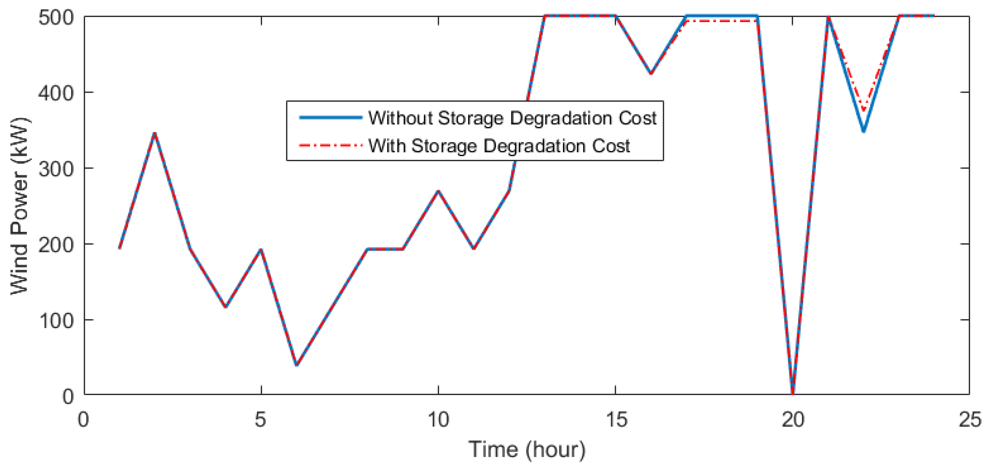
5.1. Results without BDC

The planning results concerning the hybrid WT/Battery energy system by discarding the BDC are presented using the IFLA. A comparison is made between the performance of the IFLA and conventional FLA, PSO, MRFO, and BA methods when applied to find a solution to the planning problem. The convergence process of the algorithms is given in Figure 7. As can be observed, the proposed algorithm finds the optimal solution faster than other methods and showed a better convergence performance. Additionally, the DLILS-based FLA prevents it from trapping in the local optimum points and incomplete convergence.
Table 5 lists the planning results of the hybrid WT/Battery energy system without considering the BDC using the IFLA and comparing its performance with other algorithms. According to this table, by optimal planning of the WT/Battery system, the value of each of the objectives presented in the objective function has been improved. IFLA’s proposed method has installed a wind farm with a peak size of 500 kW and a battery bank capacity of 545 kWh in Bus 7. The suggested IFLA-based planning methodology, by providing electrical planning based on battery bank charge and discharge management and power injection to the network, as well as meeting the demand of the WT/Battery system, the grid power losses decreased from 1833.62 kW to 1021.10 kW, the voltage deviations declined from value of 0.0149 p.u to 0.0055 p.u, and also the ENS decreased from 93.59 MWh to 63.22 MWh, which has provided the positive performance of the planning method in improving the objectives. The net present cost in the proposed methodology based on IFLA is obtained SAR 2,080,567.32. By comparing the numerical performance of the IFLA with the FLA, PSO, MRFO, and BA methods, in addition to achieving a lower cost value, the IFLA has improved each of the objectives. The comparison of the statistical analysis of different algorithms with 30 independent implementations is given in Table 6, which shows that the IFLA has achieved better statistical values compared to other methods, achieving lower values of mean, best, and STD.

5.2. Results with BDC

The planning results of the hybrid WT/Battery energy system in the 33-bus distribution system are given hoping to minimize the power losses, improve the network voltage profile, increase the reliability level, and minimize the net present cost together with BDC using the IFLA. The convergence trend of the IFLA and other algorithms can be seen in Figure 8. The suggested approach has obtained convergence in less iterations and has achieved the optimal solution with faster convergence and smaller convergence tolerance. Additionally, the performance improvement of the conventional FLA based on the DLILS method by avoiding local optima is quite evident.
The results obtained for the hybrid WT/Battery system planning in the 33-bus distribution system considering BDC using IFLA are presented in Table 7 and a comparison is made between IFLA and FLA, PSO, MRFO, and BA methods. As is observed, optimal planning of the hybrid WT/Battery energy system has reduced power losses, voltage deviations, as well as ENS value compared to the basic network. The proposed methodology based on the IFLA has installed a wind farm with a peak size of 500 kW and a battery capacity of 325 kWh in Bus 7 of the network. Considering the battery storage integrated with wind energy resources has led to an electrical planning implementation according to the battery reserve power and injection of the power to the network, the power loss of the network decreased from 1833.62 kW to 1072.85 kW, the voltage deviations decreased from 0.0149 p.u to 0.0057 p.u, and the ENS value declined from 93.59 MWh to 68.45 MWh. Moreover, the total NPC is obtained SAR 2,092,928.86 and the cost of battery degradation is achieved SAR 62,372.09 using the IFLA. Comparing the results of the IFLA algorithm with the FLA, PSO, MRFO, and BA methods has shown that the proposed IFLA achieves a lower objective function value and minimum values of losses, voltage deviations, and ENS. The statistical analysis of different methods performance with 30 independent executions is presented in Table 8. The IFLA obtained better values of mean, best, and STD criteria and confirmed the better performance of the IFLA-based approach of this paper.

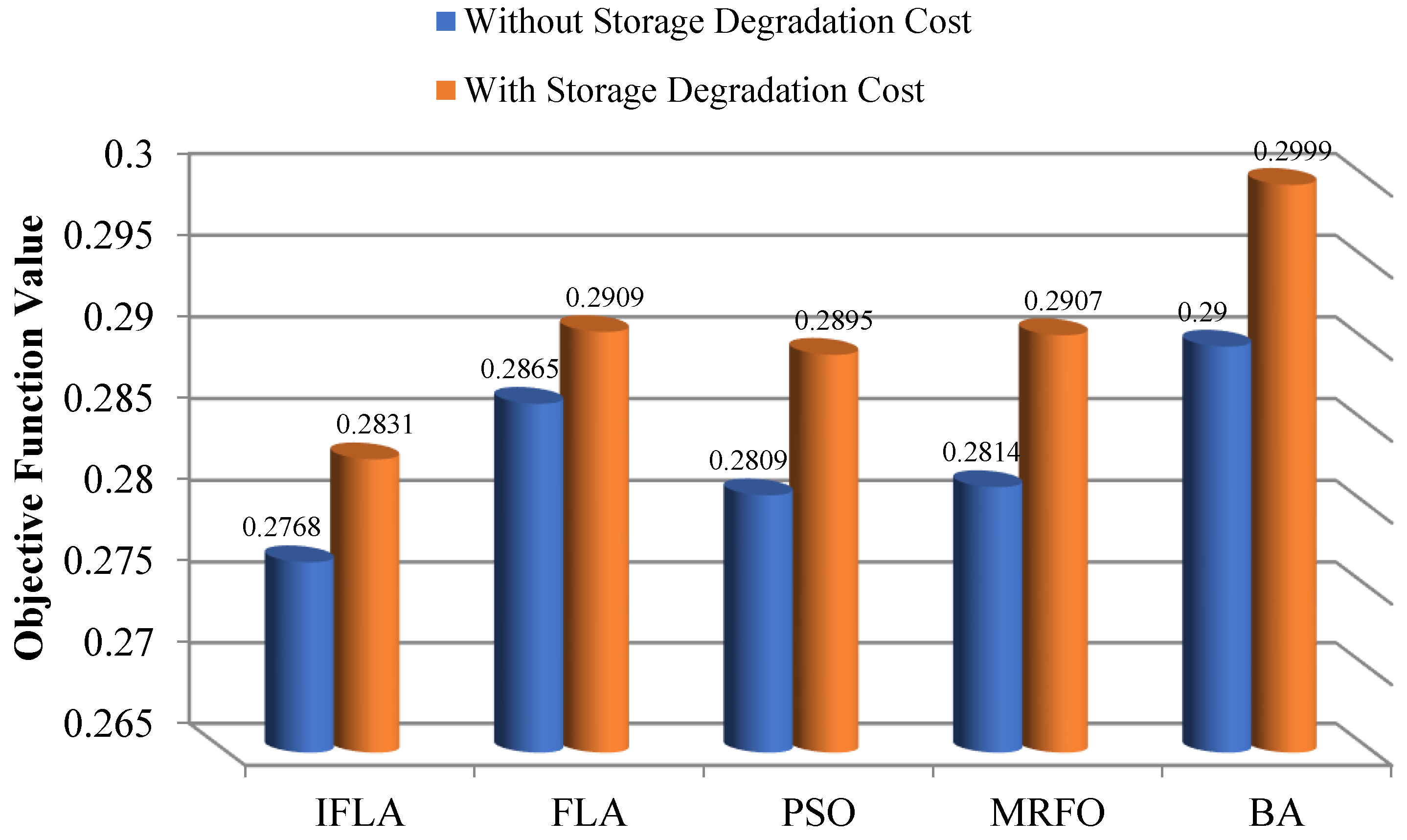
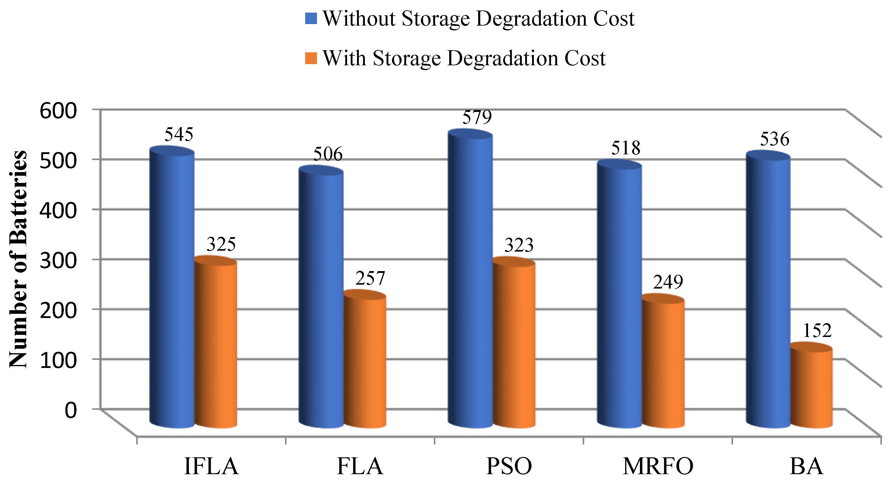
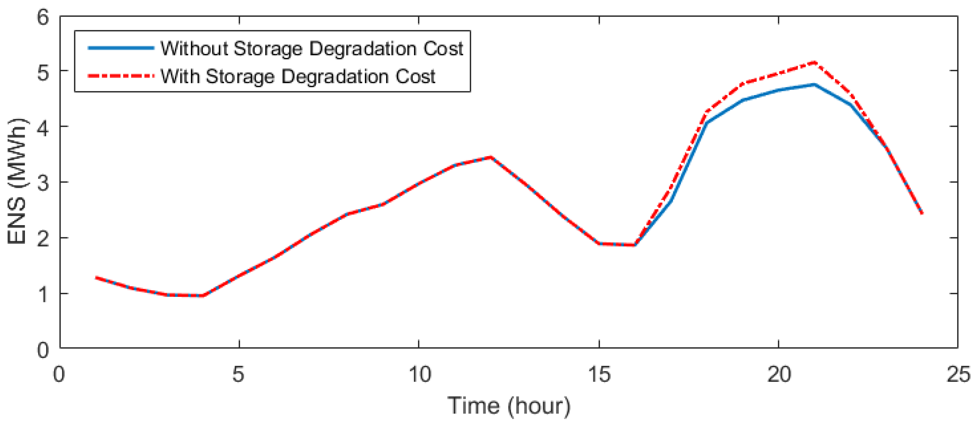
5.3. Comparison of Results

The optimal planning results of the hybrid WT/Battery energy system in the 33-bus distribution network without and with BDC including objective function value, the number of batteries, wind farm power, battery bank reserve energy, power loss, voltage oscillations of the system, and ENS values have been compared. In Figure 9, the objective function value obtained from the planning of the WT/Battery HES is compared in two cases: inclusion of BDC and exclusion of it. It is evident that considering the BDC, the objective function value has been weakened by all the methods. According to the results obtained in Table 5, Table 6, Table 7 and Table 8, in case of exclusion of BDC, the power losses, voltage deviations, and ENS are reduced by 44.31%, 63.08%, and 32.45%, respectively, compared to the base network and these objectives are decreased by 41.49%, 61.74%, and 26.86%, respectively compared to the base network in case of considering BDC. The comparison shows that when considering the BDC, the values of losses, voltage deviations, and ENS have increased by 2.82%, 1.34%, and 5.59%, respectively, compared to the case of without this cost. According to Figure 10, the number of batteries is reduced by considering the BDC. The wind power has decreased in some hours in Figure 11, and in Figure 12, the energy stored in the battery bank has decreased significantly due to the decrease in the number of batteries between 19.00 and 24.00 h considering the BDC. In addition, according to Figure 13 and Figure 14, considering the BDC, the losses and ENS have been increased (weakened) compared to the case without the BDC. Additionally, according to Figure 15, considering the BDC, the voltage oscillations of some buses has increased compared to exclusion of the BDC. Therefore, it is concluded that considering the BDC in the use of battery storage in the 24 h time horizon in solving the multi-objective hybrid WT/Battery system planning reduced the system storage level and weakened each of the objectives. Therefore, the consideration of the BDC in the detailed planning of energy systems based on battery storage, in addition to providing a more accurate model than without considering the BDC, makes the designers of these types of systems aware of the energy generation cost, and the awareness of system planners helps to make accurate decisions to meet the network demand considering power purchase from the HES integrated with battery storage.

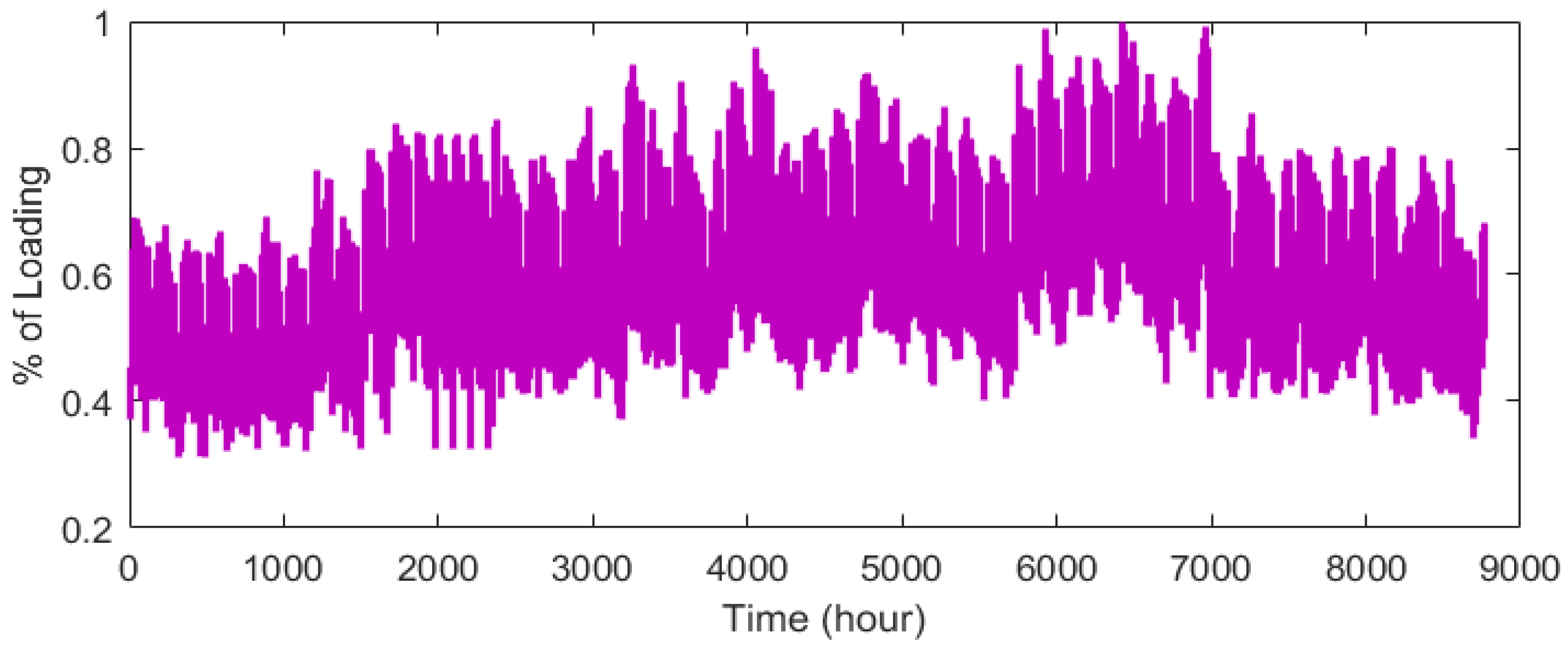
5.4. Long-Term Scheduling Results with BDC

The annual scheduling results of the hybrid WT/Battery energy system in the 33-bus distribution system are presented to minimize the power losses, improve the network voltage profile, increase the reliability level, and minimize the net present cost together with BDC using the IFLA considering 8760 h. Annual profile of wind speed, hybrid system demand, and also percentage of network peak load for 8760 h are depicted in Figure 16, Figure 17 and Figure 18, respectively. Additionally, the IFLA results are presented in Table 9.
The annual results obtained for the hybrid WT/Battery system scheduling in the 33-bus distribution system considering BDC using IFLA are presented in Table 9. The IFLA has installed a wind farm with a peak size of 500 kW and a battery capacity of 568 kWh in Bus 27 of the network. The power loss of the network decreased from 689,110.61 kW to 452,410.33 kW, the voltage deviations decreased from 0.0143 p.u to 0.0102 p.u, and the ENS value declined from 100.56 MWh to 74.82 MWh in a year. Moreover, the the cost of battery degradation is achieved 109,127.31 using the IFLA. Therefore, the results obtained from long-term scheduling have confirmed the optimal performance of the proposed methodology based on the IFLA in reducing network losses and voltage deviations, as well as improving the reliability of network customers.

5.5. Comparison with the Past Research

In [41] and [42], allocation a 3 MW wind turbine is developed to make power loss minimized and smooth the voltage profile in the 33-bus distribution system by adopting the genetic algorithm (GA) [41] and backtracking search optimization algorithm (BSOA) [42], and the IFLA results while using a turbine with a peak capacity of 500 kW along with a battery bank are compared with [41,42] in Table 10. As can be seen, compared to the GA and BSOA, the IFLA has obtained a lower losses value despite the use of energy sources with a lower capacity but integrated with battery storage. In addition, in these studies, reliability assessment has not been performed, but in the present approach, the customers reliability level has also been improved.

6. Conclusions

The current study concerns the multi-objective planning of a hybrid WT/Battery energy system in a 33-bus distribution system and attempts to minimize power loss, smooth the voltage profile, enhance reliability, and minimize the hybrid system net present cost and the BDC. The new IFLA algorithm based on the DLILS assists to specify decision variables including the planning problem. The planning problem without and considering the BDC is solved using the IFLA and compared with the results of the FLA, PSO, MRFO, and BA methods. As per the findings, based on the reserve power management of the battery storage system, electrical planning was established to constantly meet the load and optimally inject power to the distribution network to enhance the quality of objectives. The results demonstrated that the IFLA compared to other methods leads to higher drop of power loss, and further smoothness of the voltage profile and enhanced reliability. According to statistical analysis, the use of the DLILS in boosting the suggested method prevents premature convergence of the conventional FLA. Additionally, it is found that inclusion of the BDC in the storage system decreases the level of reserve energy and increases power loss and voltage oscillations, as well as weakens the reliability.
Moreover, considering the BDC, the losses, voltage deviations, and ENS have increased by 2.82%, 1.34%, and 5.59%, respectively, compared to the case without the BDC. Therefore, considering the BDC in the HES planning with battery storage makes planners of distribution networks more aware of the exact level of losses, voltage deviations, as well as reliability variations due to purchasing power from these energy systems, and prevents the planners from making wrong decisions to logically enhance the features of the distribution system.

Author Contributions

All the authors contributed to formulating the research idea, algorithm design, result analysis, writing, and reviewing the research. All authors have read and agreed to the published version of the manuscript.

Funding

This work was funded by the Deanship of Scientific Research at Jouf University under Grant Number DSR2022-RG-0113.

Data Availability Statement

Data sharing is not applicable—no new data are generated.

Conflicts of Interest

The authors declare no conflict of interest.

Nomenclature

E i Voltage of bus i
E j Voltage of bus j
E i min Minimum voltage of buses
E i max Maximum voltage of buses
I k Passing current through line k
i k d i p Best solution for the ith person
M Number of components contained in the knowledge
mMean value
M C i j Current passing through the network lines
M C i j N o m i n a l Allowable current passing through the network lines
NNumber of buses
N b Number of network lines
N p number of populations
NsampSample number of monte carlo simulation
P d Active load demand
P D G max Maximum active power of DG
P l o s s Total active power losses
P l o s s k Active power losses magnitude at line k
P m + 1 Active power of bus m + 1
P p o s t Active power of post
P P V PV power
p r Random exploratory learning probability
P r a t e d Rated PV power
Q d Reactive load demand
Q D G DG reactive power payments
Q D G min Minimum reactive power of DG
Q D G m a x Maximum reactive power of DG
Q l o s s Total reactive power losses of the network lines
Q l o s s k Reactive power losses magnitude at line k
Q m + 1 Active power of bus m + 1
Q p o s t Reactive power of post
R g Position resulting from the mutation process
R k Resistance of line k
R max , R min Lower and upper values of the variables
randA number in the range [0, 1)
S l o s s Total apparent power losses
S l o s s a f t e r _ P V s Apparent losses with PVs
S l o s s b e f o r e _ P V s Apparent losses without PVs
skdqSocial knowledge of qth in SKD
stStandard deviation
V D t o t a l Total voltage deviations
V D t o t a l a f t e r _ P V s Voltage deviations with PVs
V D t o t a l b e f o r e _ P V s Voltage deviations without PVs
V S I Voltage stability index
V S I t o t a l a f t e r _ P V s VSI with PVs
w 1 ,   w 2 ,   w 3 Weighted coefficients of three objectives
X i j ith person
X k Reactance of line k
ϕ Irradiance
ϕ r e f Reference irradiance
η M P P T PV MPPT efficiency
f b ϕ stochastic PDF of beta
ξ , ψ beta PDF parameters
μ Mean value in PDF of beta
Ω Deviation value in PDF of beta

Appendix A

Steps of implementation of the FLA.
Algorithm A1. FLA
1: Initialization;
2: Insert parameters of D, C1, C2, C3, C4, C5;
3: Initiate the population Xi (i = 1, 2 … N) as random;
4: Clustering: Dividing the population into two groups N1, and N2;
5: for s = 1:2 do
6:  Calculate the fitness of each group molecule Ns;
7:  Determining the best molecule is the best fitness value;
8: end for
9: while FES ≤ MAXFES do
10:   if If TF is greater than 0.9 then: (SSO)
11:     for op = 1: nop do
12:      Compute rate of diffusion via Equation (48)
13:      Compute the step of motion factor via Equation (49)
14:      Update position of the population via Equation (46)
15:     end for
16:   else if If TF is fewer than rand then (EO)
17:      for op = 1: nop do
18:      Compute rate of diffusion via Equation (39)
19:      Compute quantity of group relative via Equation (38)
20:      Update position of the population via Equation (37)
21:     end for
22:  else (EO)
23:     Compute flow direction via Equation (31)
24:     Calculate molecules number tending to move to region via Equation (28)
25:     Update position of the population via Equation (30);
26:     Update remained molecules in the region i via Equation (35);
27:     Update the region j molecules via Equation (36);
28:  Update FES ← FES + NP;
29: end while
30: Return best solution; = 0

References

  1. Hadidian-Moghaddam, M.J.; Arabi-Nowdeh, S.; Bigdeli, M.; Azizian, D. A multi-objective optimal sizing and siting of distributed generation using ant lion optimization technique. Ain Shams Eng. J. 2018, 9, 2101–2109. [Google Scholar] [CrossRef]
  2. Naderipour, A.; Abdul-Malek, Z.; Nowdeh, S.A.; Ramachandaramurthy, V.K.; Kalam, A.; Guerrero, J.M. Optimal allocation for combined heat and power system with respect to maximum allowable capacity for reduced losses and improved voltage profile and reliability of microgrids considering loading condition. Energy 2020, 196, 117124. [Google Scholar] [CrossRef]
  3. Farhat, O.; Khaled, M.; Faraj, J.; Hachem, F.; Taher, R.; Castelain, C. A short recent review on hybrid energy systems: Critical analysis and recommendations. Energy Rep. 2022, 8, 792–802. [Google Scholar] [CrossRef]
  4. Jahannoush, M.; Nowdeh, S.A. Optimal designing and management of a stand-alone hybrid energy system using meta-heuristic improved sine–cosine algorithm for Recreational Center, case study for Iran country. Appl. Soft Comput. 2020, 96, 106611. [Google Scholar] [CrossRef]
  5. Naderipour, A.; Kamyab, H.; Klemeš, J.J.; Ebrahimi, R.; Chelliapan, S.; Nowdeh, S.A.; Abdullah, A.; Marzbali, M.H. Optimal design of hybrid grid-connected photovoltaic/wind/battery sustainable energy system improving reliability, cost and emission. Energy 2022, 257, 124679. [Google Scholar] [CrossRef]
  6. Alanazi, A.; Alanazi, M.; Nowdeh, S.A.; Abdelaziz, A.Y.; El-Shahat, A. An optimal sizing framework for autonomous photovoltaic/hydrokinetic/hydrogen energy system considering cost, reliability and forced outage rate using horse herd optimization. Energy Rep. 2022, 8, 7154–7175. [Google Scholar] [CrossRef]
  7. Paudel, S.; Shrestha, J.N.; Neto, F.J.; Ferreira, J.A.; Adhikari, M. Optimization of hybrid PV/wind power system for remote telecom station. In Proceedings of the 2011 International Conference on Power and Energy Systems (ICPS), Chennai, India, 22–24 December 2011; pp. 1–6. [Google Scholar]
  8. Nagabhushana, A.C.; Jyoti, R.; Raju, A.B. Economic analysis and comparison of proposed HRES for stand-alone applications at various places in Karnataka state. In Proceedings of the ISGT2011-India, Kollam, India, 1–3 December 2011. [Google Scholar]
  9. La Terra, G.; Salvina, G.; Tina, G.M. Optimal sizing procedure for hybrid solar wind power systems by fuzzy logic. In Proceedings of the MELECON 2006–2006 IEEE Mediterranean Electrotechnical Conference, Malaga, Spain, 16–19 May 2006; pp. 865–868. [Google Scholar]
  10. Xu, D.; Kang, L.; Chang, L.; Cao, B. Optimal sizing of standalone hybrid wind/PV power systems using genetic algorithms. In Proceedings of the Canadian Conference on Electrical and Computer Engineering, Saskatoon, SK, Canada, 4 May 2005; pp. 1722–1725. [Google Scholar]
  11. Zhao, Y.S.; Zhan, J.; Zhang, Y.; Wang, D.P.; Zou, B.G. The optimal capacity configuration of an independent wind/PV hybrid power supply system based on improved PSO algorithm. In Proceedings of the 8th International Conference on Advances in Power System Control, Operation and Management (APSCOM 2009), Hongkong, China, 8–11 November 2009. [Google Scholar]
  12. Jemaa, A.B.; Hamzaoui, A.; Essounbouli, N.; Hnaien, F.; Yalawi, F. Optimum sizing of hybrid PV/wind/battery system using Fuzzy-Adaptive Genetic Algorithm. In Proceedings of the 2013 3rd International Conference on Systems and Control (ICSC), Algiers, Algeria, 29–31 October 2013; pp. 810–814. [Google Scholar]
  13. Tutkun, N.; San, E.S. Optimal power scheduling of an off-grid renewable hybrid system used for heating and lighting in a typical residential house. In Proceedings of the 2013 13th International Conference on Environment and Electrical Engineering (EEEIC), Wroclaw, Poland, 1–3 November 2013; pp. 352–355. [Google Scholar]
  14. Dehghan, S.; Saboori, H.; Parizad, A.; Kiani, B. Optimal sizing of a hydrogen-based wind/PV plant considering reliability indices. In Proceedings of the International Conference on Electric Power and Energy Conversion Systems, 2009. EPECS’09, Sharjah, United Arab Emirates, 10–12 November 2009; pp. 1–9. [Google Scholar]
  15. Sánchez, V.; Ramirez, J.M.; Arriaga, G. Optimal sizing of a hybrid renewable system. In Proceedings of the 2010 IEEE International Conference on Industrial Technology (ICIT), Via del Mar, Chile, 14–17 March 2010; pp. 949–954. [Google Scholar]
  16. Bansal, A.K.; Gupta, R.A.; Kumar, R. Optimization of hybrid PV/wind energy system using Meta Particle Swarm Optimization (MPSO). In Proceedings of the 2010 India International Conference on Power Electronics (IICPE), New Delhi, India, 28–30 January 2011; pp. 1–7. [Google Scholar]
  17. Bashir, M.; Sadeh, J. Size optimization of new hybrid stand-alone renewable energy system considering a reliability index. In Proceedings of the 2012 11th International Conference on Environment and Electrical Engineering (EEEIC), Venice, Italy, 18–25 May 2012; pp. 989–994. [Google Scholar]
  18. Sanchez, V.M.; Chavez-Ramirez, A.U.; Duron-Torres, S.M.; Hernandez, J.; Arriaga, L.G.; Ramirez, J.M. Techno-economical optimization based on swarm intelligence algorithm for a stand-alone wind-photovoltaic-hydrogen power system at south-east region of Mexico. Int. J. Hydrog. Energy 2014, 39, 16646–16655. [Google Scholar] [CrossRef]
  19. Fathy, A.; Kaaniche, K.; Alanazi, T.M. Recent approach based social spider optimizer for optimal sizing of hybrid PV/wind/battery/diesel integrated microgrid in Aljouf region. IEEE Access 2020, 8, 57630–57645. [Google Scholar] [CrossRef]
  20. Mohammed, A.Q.; Al-Anbarri, K.A.; Hannun, R.M. Optimal Combination and Sizing of a Stand–Alone Hybrid Energy System Using a Nomadic People Optimizer. IEEE Access 2020, 8, 200518–200540. [Google Scholar] [CrossRef]
  21. Jafar-Nowdeh, A.; Babanezhad, M.; Arabi-Nowdeh, S.; Naderipour, A.; Kamyab, H.; Abdul-Malek, Z.; Ramachandaramurthy, V.K. Meta-heuristic matrix moth–flame algorithm for optimal reconfiguration of distribution networks and placement of solar and wind renewable sources considering reliability. Environ. Technol. Innov. 2020, 20, 101118. [Google Scholar] [CrossRef]
  22. Nowdeh, S.A.; Davoudkhani, I.F.; Moghaddam, M.H.; Najmi, E.S.; Abdelaziz, A.Y.; Ahmadi, A.; Razavi, S.E.; Gandoman, F.H. Fuzzy multi-objective placement of renewable energy sources in distribution system with objective of loss reduction and reliability improvement using a novel hybrid method. Appl. Soft Comput. 2019, 77, 761–779. [Google Scholar] [CrossRef]
  23. Ugranlı, F.; Karatepe, E. Optimal wind turbine sizing to minimize energy loss. Int. J. Electr. Power Energy Syst. 2013, 53, 656–663. [Google Scholar] [CrossRef]
  24. Dahal, S.; Salehfar, H. Impact of distributed generators in the power loss and voltage profile of three phase unbalanced distribution network. Int. J. Electr. Power Energy Syst. 2016, 77, 256–262. [Google Scholar] [CrossRef]
  25. Kayal, P.; Chanda, C.K. Placement of wind and solar based DGs in distribution system for power loss minimization and voltage stability improvement. Int. J. Electr. Power Energy Syst. 2013, 53, 795–809. [Google Scholar] [CrossRef]
  26. Safaei, A.; Vahidi, B.; Askarian-Abyaneh, H.; Azad-Farsani, E.; Ahadi, S.M. A two step optimization algorithm for wind turbine generator placement considering maximum allowable capacity. Renew. Energy 2016, 92, 75–82. [Google Scholar] [CrossRef]
  27. Ali, E.S.; Elazim, S.A.; Abdelaziz, A.Y. Ant Lion Optimization Algorithm for optimal location and sizing of renewable distributed generations. Renew. Energy 2017, 101, 1311–1324. [Google Scholar] [CrossRef]
  28. Arabi-Nowdeh, S.; Nasri, S.; Saftjani, P.B.; Naderipour, A.; Abdul-Malek, Z.; Kamyab, H.; Jafar-Nowdeh, A. Multi-criteria optimal design of hybrid clean energy system with battery storage considering off-and on-grid application. J. Clean. Prod. 2021, 290, 125808. [Google Scholar] [CrossRef]
  29. Arasteh, A.; Alemi, P.; Beiraghi, M. Optimal allocation of photovoltaic/wind energy system in distribution network using meta-heuristic algorithm. Appl. Soft Comput. 2021, 109, 107594. [Google Scholar] [CrossRef]
  30. Javad Aliabadi, M.; Radmehr, M. Optimization of hybrid renewable energy system in radial distribution networks considering uncertainty using meta-heuristic crow search algorithm. Appl. Soft Comput. 2021, 107, 107384. [Google Scholar] [CrossRef]
  31. Hashim, F.A.; Mostafa, R.R.; Hussien, A.G.; Mirjalili, S.; Sallam, K.M. Fick’s Law Algorithm: A physical law-based algorithm for numerical optimization. Knowl. Based Syst. 2023, 260, 110146. [Google Scholar] [CrossRef]
  32. Dallinger, D. Plug-in Electric Vehicles Integrating Fluctuating Renewable Electricity (Vol. 20); Kassel University Press GmbH: Kassel, Germany, 2013. [Google Scholar]
  33. Chang, W.Y. The state of charge estimating methods for battery: A review. In International Scholarly Research Notices; Hindawi Publishing: New York, NY, USA, 2013. [Google Scholar]
  34. Gong, M.; Zhang, M.; Yuan, Y. Unsupervised band selection based on evolutionary multiobjective optimization for hyperspectral images. IEEE Trans. Geosci. Remote Sens. 2015, 54, 544–557. [Google Scholar] [CrossRef]
  35. Lotfipour, A.; Afrakhte, H. A discrete Teaching–Learning-Based Optimization algorithm to solve distribution system reconfiguration in presence of distributed generation. Int. J. Electr. Power Energy Syst. 2016, 82, 264–273. [Google Scholar] [CrossRef]
  36. Long, W.; Jiao, J.; Xu, M.; Tang, M.; Wu, T.; Cai, S. Lens-imaging learning Harris hawks optimizer for global optimization and its application to feature selection. Expert Syst. Appl. 2022, 202, 117255. [Google Scholar] [CrossRef]
  37. Zhao, W.; Zhang, Z.; Wang, L. Manta ray foraging optimization: An effective bio-inspired optimizer for engineering applications. Eng. Appl. Artif. Intell. 2020, 87, 103300. [Google Scholar] [CrossRef]
  38. Kennedy, J.; Eberhart, R. Particle swarm optimization. In Proceedings of the ICNN’95-International Conference on Neural Networks, Perth, Australia, 27 November 1995; Volume 4, pp. 1942–1948. [Google Scholar]
  39. Baran, M.E.; Wu, F.F. Network reconfiguration in distribution systems for loss reduction and load balancing. IEEE Trans. Power Deliv. 1989, 4, 1401–1407. [Google Scholar] [CrossRef]
  40. Ahmadi, S.; Abdi, S. Application of the Hybrid Big Bang–Big Crunch algorithm for optimal sizing of a stand-alone hybrid PV/wind/battery system. Sol. Energy 2016, 134, 366–374. [Google Scholar] [CrossRef]
  41. Hassan, A.A.; Fahmy, F.H.; Nafeh, A.E.S.A.; Abu-elmagd, M.A. Genetic single objective optimisation for sizing and allocation of renewable DG systems. Int. J. Sustain. Energy 2017, 36, 545–562. [Google Scholar] [CrossRef]
  42. El-Fergany, A. Optimal allocation of multi-type distributed generators using backtracking search optimization algorithm. Int. J. Electr. Power Energy Syst. 2015, 64, 1197–1205. [Google Scholar] [CrossRef]
Figure 1. Interconnection of the hybrid WT/Battery energy system and the radial distribution system.
Mathematics 11 01270 g001
Figure 2. Dynamic lens-imaging learning strategy.
Mathematics 11 01270 g002
Figure 3. Schematic of the 33-bus distribution system.
Mathematics 11 01270 g003
Figure 4. Profile of wind speed during a day.
Mathematics 11 01270 g004
Figure 5. Profile of hybrid system demand during a day.
Mathematics 11 01270 g005
Figure 6. Percentage of network peak load during a day.
Mathematics 11 01270 g006
Figure 7. The convergence process of different algorithms to solve the WT/Battery scheduling problem without storage degradation cost.
Mathematics 11 01270 g007
Figure 8. The convergence trend of various algorithms to solve the WG/Battery scheduling problem with storage degradation cost.
Mathematics 11 01270 g008
Figure 9. Value of objective function using different algorithms without and with storage degradation cost.
Mathematics 11 01270 g009
Figure 10. Number of batteries without and with BDC in WT/Battery scheduling using the IFLA.
Mathematics 11 01270 g010
Figure 11. Contribution of different components without and with BDC in WT/Battery scheduling using the IFLA.
Mathematics 11 01270 g011
Figure 12. Battery bank energy without and with BDC in WT/Battery scheduling using the IFLA.
Mathematics 11 01270 g012
Figure 13. Power losses of the network without and with BDC in WT/Battery scheduling using the IFLA.
Mathematics 11 01270 g013
Figure 14. ENS of the network without and with BDC in WT/Battery scheduling using the IFLA.
Mathematics 11 01270 g014
Figure 15. Voltage profile of the network by considering/neglecting the BDC in WT/Battery scheduling using the IFLA.
Mathematics 11 01270 g015
Figure 16. Profile of annual wind speed.
Mathematics 11 01270 g016
Figure 17. Profile of annual hybrid system demand.
Mathematics 11 01270 g017
Figure 18. Percentage of annual network peak load.
Mathematics 11 01270 g018
Table 1. Parameters of various algorithms under study.
AlgorithmParameterValue
FLA [31]D, C1, C2, C3, C4, C50.1, 5, 2, 0.1, 0.2, 2
PSO [38]Cognitive and social constant
Inertia weight
Velocity limit
(C1, C2) 2, 2
Linear reduction from 0.9 to 0.1
10% of dimension range
MRFO [37] S 2
(5)
Table 2. Mean results for classic test functions when adopting PSO, MRFO, FLA, and IFLA (the significant values are marked in boldface).
FunctionPSOMRFOFLAIFLA
F12.96 × 10−85.14 × 10−141.59 ×10−77.70 × 10−19
---
F25.59 × 10−12.38 × 10−18.95 × 10−11.72 × 10⁻¹
---
F31.67 × 1023.64 × 1016.21 × 1013.55 × 101
---
F49.614.426.562.36
---
F53.44 × 1013.07 × 1015.49 × 1012.73 × 101
---
F64.74 × 1072.55 × 10−152.99 × 10−52.71 × 10−17
---
F74.75 × 10−22.45 × 10−23.89 × 10−21.69 × 10⁻²
---
F8−8.24 × 10³−7.96 × 10³−7.51 × 10³ −8.09 × 10³
+--
F93.35 × 1013.30 × 1013.44 × 1012.97 × 101
---
F102.402.292.571.34
---
F111.72 × 10−15.02 × 10−23.97 × 10−23.73 × 10⁻²
---
F121.961.371.212.08 × 10−1
---
F131.57 × 1011.21 × 1011.34 × 1012.59
---
F149.98 × 10−19.98 × 10−19.98 × 10−19.98 × 10−1
===
F152.50 × 10−35.39 × 10−47.85 × 10−46.73 × 10⁻⁴
-+-
F16−1.03−1.03−1.03−1.03
===
F173.98 × 10−13.98 × 10−13.98 × 10−13.98 × 10−1
===
F183.003.003.003.00
===
F19−3.86−3.86−3.86−3.86
===
F20−3.27−3.24−3.27−3.29
---
F21−6.53−7.03−6.86−8.65
---
F22−5.53−8.25−7.82−8.80
---
F23−9.48−8.67−7.75−9.48
=--
Final rank2341
Table 3. The results of Wilcoxon’s test.
Corresponding AlgorithmIFDA Versus
p-ValuesBetterWorstEqual
PSO1.9644 × 10−41805
MRFO3.2701 × 10−41715
FLA3.6027 × 10−41616
Table 4. Technical information and cost of wind turbine, battery, and inverter of WT/Battery system [40].
ComponentParametersValues
WT
PWT-rated1 kW
vci3 m/s
vr13 m/s
vco20 m/s
WT lifetime20 years
WT capital cost$3200
WT replacement cost--
WT O&M cost$100/year
Battery
EBat max1 kA h
EBat min0.2 kA h
μBattery0.9
DOD0.8
Battery lifetime5 years
Battery capital cost100
Battery replacement cost--
Battery O&M cost$5/year
Inverter
μInv0.95
Table 5. The numerical results of different methods of hybrid WT/Battery system scheduling without storage degradation cost for 33-bus distribution network.
ItemProposed IFLAFLAPSOMRFOBA
Before scheduling
Power loss (kW)1833.621833.621833.621833.621833.62
Voltage Deviation (p.u)0.01490.01490.01490.01490.0149
Minimum Voltage (p.u)0.95650.95650.95650.95650.9565
ENS (MWh)93.5993.5993.5993.5993.59
After scheduling
HS Location (Bus)72727279
Size: WT/Battery (kW/kWh)500/325466/257500/323464/309421/152
Power loss (kW)1072.851110.831080.151085.101126.36
Voltage Deviation (p.u)0.00570.00680.00610.00640.0073
Minimum Voltage (p.u)0.98250.97840.98050.97930.9740
ENS (MWh/year)68.4570.1669.5169.7370.48
Storage degradation cost ((SAR/year)62,372.0939,329.4461,952.6847,749.1429,147.09
Cost of HS (SAR)2,092,928.861,950,918.582,092,874.011,946,005.471,764,784.91
OF 0.28310.29090.28950.29070.2999
Table 6. The performance comparison of different algorithms using the statistic analysis without storage degradation cost.
ItemIFLAFLAPSOMRFOBA
Best0.27680.28650.28090.28140.2900
Mean0.27750.28770.28260.28330.2927
Worst0.27880.28890.28400.28490.2951
STD0.03200.05180.04750.03630.0535
Table 7. The numerical report on different methods of hybrid WG/Battery system scheduling with storage degradation cost for 33-bus distribution system.
ItemProposed IFLAFLAPSOMRFOBA
Before scheduling
Power loss (kW)1833.621833.621833.621833.621833.62
Voltage Deviation (p.u)0.01490.01490.01490.01490.0149
Minimum Voltage (p.u)0.95650.95650.95650.95650.9565
ENS (MWh)93.5993.5993.5993.5993.59
After scheduling
HS Location (Bus)72727279
Size: WT/Battery (kW/kWh)500/325466/257500/323464/309421/152
Power loss (kW)1072.851110.831080.151085.101126.36
Voltage Deviation (p.u)0.00570.00680.00610.00640.0073
Minimum Voltage (p.u)0.98250.97840.98050.97930.9740
ENS (MWh)68.4570.1669.5169.7370.48
Storage degradation cost (SAR)62,372.0939,329.4461,952.6847,749.1429,147.09
Cost of HS (SAR)2,092,928.861,950,918.582,092,874.011,946,005.471,764,784.91
OF 0.28310.29090.28950.29070.2999
Table 8. The performance comparison of different algorithms using the statistic analysis with storage degradation cost.
ItemIFLAFLAPSOMRFOBA
Best0.28310.29090.28950.29070.2999
Mean0.28380.29230.29060.29180.3014
Worst0.28460.29310.29110.29270.3035
STD0.02160.03200.02370.03010.0528
Table 9. The annual results of IFLA for scheduling of the hybrid WG/Battery system with storage degradation cost for 33-bus distribution system.
ItemProposed IFLA
Before scheduling
Power loss (kW)689,110.61
Voltage Deviation (p.u)0.0143
Minimum Voltage (p.u)0.9582
ENS (MWh/year)100.56
Before scheduling
HS Location (Bus)27
Size: WT/Battery (kW/kWh)500/568
Power loss (kW)452,410.33
Voltage Deviation (p.u)0.0102
Minimum Voltage (p.u)0.9651
ENS (MWh/year)74.82
Storage degradation cost (SAR/year)109,127.31
Table 10. Comparison with past research.
ItemIFLAGA [41]BSOA [42]
P W G PWT = 500 kW
PBattery = 325 kWh
PWT = 2980 kWPWT = 2265 kW
LocationBus 7Bus 6Bus 8
Power Loss (kW)44.7072.6882.78
Min Voltage (p.u) 0.9565--0.9549
Disclaimer/Publisher’s Note: The statements, opinions and data contained in all publications are solely those of the individual author(s) and contributor(s) and not of MDPI and/or the editor(s). MDPI and/or the editor(s) disclaim responsibility for any injury to people or property resulting from any ideas, methods, instructions or products referred to in the content.

