
Performance Analysis of Long Short-Term Memory Predictive Neural Networks on Time Series Data

The Faculty of Engineering and Information Technology, George Emil Palade University of Medicine, Pharmacy, Science, and Technology of Târgu Mureş, 540139 Târgu Mureş, Romania
*
Author to whom correspondence should be addressed.
Mathematics 2023, 11(6), 1432; https://0-doi-org.brum.beds.ac.uk/10.3390/math11061432
Submission received: 3 February 2023
/
Revised: 12 March 2023
/
Accepted: 14 March 2023
/
Published: 15 March 2023
(This article belongs to the Special Issue Artificial Intelligence and Machine Learning Based Methods and Applications)
Abstract
:Long short-term memory neural networks have been proposed as a means of creating accurate models from large time series data originating from various fields. These models can further be utilized for prediction, control, or anomaly-detection algorithms. However, finding the optimal hyperparameters to maximize different performance criteria remains a challenge for both novice and experienced users. Hyperparameter optimization algorithms can often be a resource-intensive and time-consuming task, particularly when the impact of the hyperparameters on the performance of the neural network is not comprehended or known. Teacher forcing denotes a procedure that involves feeding the ground truth output from the previous time-step as input to the current time-step during training, while during testing feeding back the predicted values. This paper presents a comprehensive examination of the impact of hyperparameters on long short-term neural networks, with and without teacher forcing, on prediction performance. The study includes testing long short-term memory neural networks, with two variations of teacher forcing, in two prediction modes, using two configurations (i.e., multi-input single-output and multi-input multi-output) on a well-known chemical process simulation dataset. Furthermore, this paper demonstrates the applicability of a long short-term memory neural network with a modified teacher forcing approach in a process state monitoring system. Over 100,000 experiments were conducted with varying hyperparameters and in multiple neural network operation modes, revealing the direct impact of each tested hyperparameter on the training and testing procedures.
Keywords:
long short-term memory (LSTM); recurrent neural network (RNN); teacher forcing; prediction; performance analysis; benchmarking; machine learning; Tennessee Eastman process; time seriesMSC:
68T07; 68T091. Introduction
Machine learning algorithms, nowadays, are a “go-to” for solving a plethora of real-life problems in various domains, from healthcare [1], finance [2], and manufacturing [3] all the way to agriculture [4]. On a larger scale, machine learning can be regarded as an umbrella term incorporating a wide range of algorithms and models proposed for specific tasks, including medical diagnosis [5], predictive maintenance [6], text authorship attribution [7], human race recognition [8], and anomaly detection [9].
One specific subclass of machine learning includes neural networks. Since the first mention of artificial neurons almost 80 years ago [10], neural networks have constantly evolved and have been widely applied in numerous areas and domains, from economics [11] to medicine [12,13,14] to industrial domains [15]. Long short-term memory (LSTM) neural networks [16] are a special type of recurrent neural networks, initially proposed as a solution to the vanishing and exploding gradient problem. As predictors, LSTM neural networks are efficient in learning long- and short-term spatio-temporal dependencies in time series data. In the scientific literature, LSTMs have been proposed for prediction tasks on time series data in a multitude of papers [17,18,19,20]. Moreover, LSTMs have also been used for other task as well, such as text classification [21], phoneme classification [22], time series classification [19,23], electroencephalogram (EEG) classification [24], remaining useful life prediction [25], and sentiment analysis [26,27].
One major difficulty when working with neural networks is discovering the optimal hyperparameters [28] or the best-suited model for optimal performance. To this day, optimizing the hyperparameters involves finding the best values for specific datasets and for specific network architectures. Among the well-known optimization techniques, we find the grid search method [29], a blackbox hyperparameter optimization method involving finding the best values from a finite set. An alternative to grid search is random search [29], which involves randomly sampling hyperparameter values based on a search budget. Another popular optimization technique is Bayesian optimization [29], a technique that involves using a surrogate model to approximate a complex function and an acquisition function to determine the next point to evaluate. It operates through an iterative process, with the surrogate model and acquisition function being updated at each step.
The performance of neural networks has been analyzed by numerous researchers in diverse domains and on a multitude of datasets [30,31,32,33,34,35,36,37,38,39]. The classification and prediction performance of neural networks has been shown to be influenced by various factors, such as the architecture, the hyperparameters, and the dataset. While optimization techniques aid in discovering the best hyperparameters for such models, oftentimes an in-depth performance analysis is needed to observe and understand how different hyperparameters actually affect the functionality of the neural networks. Moreover, considering the high usability of neural networks by expert and novice users alike, oftentimes running an optimization algorithm (which can be time- and resource-consuming) is not enough without observing the model behavior.
This paper focuses on a prediction performance comparison between standard LSTMs and LSTMs trained with two variants of teacher forcing (TF) used for time series prediction in a process state monitoring system. The two variants of TF include the one proposed in [40] for anomaly-detection tasks (LSTMTF) and, as originally proposed in [41], for long-term forecasting (LSTMTFC).
By using an empirical approach, this paper analyzes the effects of different hyperparameters, such as the input sequence length, the number of time delays, the mini-batch size, the learning rate, and the number of hidden units, while training and testing the LSTM variants on time series data originating from an industrial process, namely, on the Tennessee Eastman process dataset [42,43]. Additionally, this paper also analyzes different neural network configurations, namely, multi-input single-output (MISO) and multi-input multi-output (MIMO) on two prediction modes, that is, many-to-many (M2M) and many-to-one (M2O). The performance analysis focuses on both the training and inference.
The prediction performance of different variants of LSTM was compared with the nonlinear auto-regressive neural networks with exogenous inputs (NARXNN). The authors of some large-scale studies, such as those in [30,31,32,35], performed thousands of experiments in this direction. For this study, approximately 100,000 neural networks were trained and tested using a wide range of hyperparameters, configurations, and prediction modes.
To the best of our knowledge, this is the first study focusing on time series prediction benchmarking of LSTM neural networks trained with TF compared to standard LSTMs. Furthermore, this paper also studies the exposure bias effect [44,45] for neural networks trained with TF in its original form. While exposure bias can affect the prediction performance of neural networks, we will also discuss the gained advantages of using LSTMs with TF for anomaly-detection tasks.
The remainder of the paper is organized as follows. Section 2 describes related studies, with special emphasis on concepts such as TF; the similarities between TF, NARXNN, and other recurrent neural networks; and hyperparameter optimization methods. The proposed approach is presented in Section 3. This is followed by Section 4, where the experimental assessment is presented. Section 5 describes the experimental results. Discussions, final remarks, and future work proposals are included in Section 6.
2. Related Work
An examination of the literature reveals a multitude of papers addressing the issues discussed throughout this paper. Thus, the related work section is split in three subsections. First, a background on teacher forcing is presented. Second, studies and benchmark papers on the topic of LSTM neural networks and recurrent neural networks (RNNs) are presented, addressing both predictive and classification tasks. Last, several highly cited hyperparameter optimization papers are investigated, while some proposed techniques from these papers are experimentally validated in the results section.
2.1. Teacher Forcing Background
We observed numerous similarities between LSTM with TF, Jordan neural networks [46], and NARXNN [35,47]. For a better understanding of the rest of this paper, the current section describes the similarities and differences between the previous terms as well as their applicability.
Recurrent neural networks, or RNNs, are neural networks that map sequence inputs to sequence outputs statefully. This means the output prediction depends not only on the input, but also on the hidden state of the system, which is updated as the sequence is processed over time [44,48,49]. Adding feedback loops to a feedforward neural network can be carried out using two fundamental approaches. The first approach is adding a feedback loop from the hidden layer to itself (or to the input layer); this resembles the Elman architecture, as originally proposed in [50]. Such an approach emphasizes, to a larger degree, the sequence of input values. The second approach is adding a feedback loop from the output layer to the input layer. This approach was first proposed in the Jordan neural network (JNN) architecture [46]. Compared to the Elman neural networks, this approach emphasizes the sequence of output values to a larger degree [48]. In the case of JNN, the previous output with only one time delay is fed back.
NARXNN denotes a special type of feedforward neural network where static backpropagation can be used for training, reducing the training phase time and resources compared to recurrent neural networks. One similarity between JNN and NARXNN is that both network architectures take exogenous variables as inputs, together with previous outputs as additional inputs. In the case of NARXNN, multiple time-steps from the output can be added as input. Additionally, NARXNN can take the exogenous variables as inputs with additional time delays (e.g., lags). NARXNNs are usually used in the engineering field for such tasks as dynamic system modeling, system identification, and particularly in the field of time series analysis.
TF was first proposed in [41], where the authors describe a training method that involves feeding back the current ground truth values as input in the subsequent time-steps. This way forces the neural network to remain as close as possible to the ground truth sequences. In recent years, several variants of TF have been proposed [51,52,53,54,55], most of them offering variations of this method for training recurrent neural networks (RNNs). In Goodfellow’s book [44], TF was also introduced as a neural network training technique, applicable to recurrent neural networks that have output to hidden connections. This technique originates from the maximum likelihood criterion, where during the training phase, the neural network receives the ground truth value of the output as input at the next time-step.
Moreover, Goodfellow et al. in [44] state that TF is also applicable to models that have hidden-to-hidden connections as well. In this scenario, training is carried out using both TF and backpropagation through time (BPTT) [56,57,58].
TF has been applied in several domains for solving diverse problems [59,60,61,62,63,64,65] (in order of appearance). Apart from the original version of the algorithm, several variations have also been proposed, a large majority of them for training RNNs.
Toomarian et al. [59] patented, for NASA, a variant of TF for fast temporal neural learning applied in circular trajectory learning. The patent proposes a continuous form of TF that modifies the activation dynamics of additive neural networks, where rather than the actual value of the output variable, the error between the desired output and the actual output is fed back to the neural network in real time.
In the same direction of trajectory learning, Toomarian and Barhen [65] also proposed a methodology for supervised temporal learning in nonlinear neural networks. Their work incorporates TF and adjoint operators for fast circular trajectory learning. This version of TF is applied similarly to the one in [59] by feeding back the error between the actual and predicted value.
To avoid exposure bias when training models with TF, Taigman et al. [51] proposed a modification to the TF algorithm, where, during training the neural network does not take the previous observed value as input, but rather, an average between the observed value and the previous network outputs with the addition of random noise. Their solution is proposed as a text-to-speech method for mimicking voices from samples originating from the wild.
Moving towards the field of language modeling, we find the work of Drossos et al. [52]. Here, the authors propose a sound event detection recurrent neural network capable of learning language models. TF is applied here using a scheduled sampling approached, that is, during the training process, gradually, based on a probability, the observed values are replaced by the outputs of the model.
A multi-domain (e.g., language modeling, vocal synthesis, image, and handwriting generation) proposed solution using a generative adversarial network with a variation of TF is the work of Lamb et al. [66], namely, Professor forcing. Their approach entails training additional discriminators to differentiate free running from forced hidden states. This approach assures that the dynamic of the network will remain similar when using observed and freely sampled values during the training procedures.
Moving towards NARXNN-based proposed solutions, we find the work of Massaoudi et al. [55] with a photovoltaic power forecasting technique. Their solution encompasses a hybrid model consisting of an LSTM neural network and an NARXNN. The NARXNN gathers data and generates a residual error vector. This vector is then fed into an LSTM neural network as additional input, allowing the LSTM to produce both point-by-point and sequence forecasts. This combination of the NARXNN model and the LSTM allows for the generation of accurate and reliable forecasts.
A popular solution that highlights the similarities between neural networks with TF and NARXNN is Amazon’s DeepAR [67]. DeepAR is a probabilistic forecasting technique that uses autoregressive RNNs to make predictions. It works by incorporating likelihoods and using nonlinear data transformation techniques, as learned by a neural network, to accurately forecast future outcomes. DeepAR is built upon an RNN where the input of the model consists of a combination of lagged target values and covariates. The model outputs either a point-by-point prediction with a standard loss function or a probabilistic prediction using the parameters of a probability density function (e.g., the mean and standard deviation value).
Other applications of NARXNN-based techniques, most of them in the energetic field, include: building temperature and energy forecasting [68,69], daily solar radiation prediction [70], load forecast for residential low-voltage distribution networks [71], hydrometeorological drought forecasting in hyper-arid climates [72], transformer oil-dissolved gas concentration prediction [73], electrical grid short-term load forecasting [74], lithium-ion battery state of health (SoH) estimation [75], and wind power prediction [76].
2.2. Neural Network Benchmarking Papers and Studies
Thomas Brueuel, from Google’s research team, studied the behavior and performance of LSTM classifiers in [30]. This study analyses the behavior of LSTMs for different hyperparameters, but also how the choice of non-linearities affects performance. Among the tested hyperparameters we find the learning rate, number of hidden units, and mini-batch size. The study focused on digit classification on two popular benchmarking datasets, namely, MNIST, which is an isolated digit handwriting classification dataset, and UW3, which is an OCR evaluation database. The results showed that the performance of LSTM classifiers mostly depends on learning rates, batching had little to no effect on performance, softmax training yielded better results compared to the least square training, and LSTMs without peephole connections obtained the best performance in comparison to LSTMs with peepholes.
Another large-scale study, on the performance of LSTM, is the work of Greff et al. [31]. Their study, named “LSTM: A search space odyssey”, analyzed the performance of eight LSTM variants on three tasks: speech recognition, handwriting recognition, and polyphonic music modeling. The studied LSTM variants included No input gate, No forget gate, No output gate, No input activation function, No output activation function, Coupled input and forget gate, No peepholes, and Full gate recurrence. As for activation functions, the standard approach was followed, namely using the sigmoid and the hyperbolic tangent functions. The authors also studied the effects of hyperparameters on the performance of the neural networks, hyperparameters such as the hidden layer size, learning rate, momentum, and input noise. However, the hyperparamter effects were not tested on entire ranges of possible values, but rather using random searches in specific ranges. The findings of this study show that the learning rate had the largest effect on the experiments, followed by the hidden layer size, and an interesting finding showed that adding noise to the inputs decreased the performance and increased the training time. One unexpected result, as the authors state, was that momentum had no effect on the performance or the training time of any of the eight tested LSTM variants. One conclusion of the study reveals that the standard LSTM variant (i.e., VLSTM) performed equally well in comparison to the other tested variants.
In a more recent study, Siami-Namini et al. [32] analyzed the time series forecasting performance of unidirectional LSTMs and bidirectional LSTMS (BiLSTMs). The authors compared the performance of auto-regressive integrated moving average (ARIMA) models, LSTMs, and BiLSTMs in the context of predicting financial time series data. One interesting aspect of this research is the prediction performance when the time series data are learned in both directions (i.e., past-to-future and future-to-past). Their results showed that BiLSTM’s training time was slower, but outperformed the unidirectional LSTM and ARIMA models in terms of prediction accuracy. Nonetheless, the authors provided no architectural or hyperparameter information about the tested neural networks, or whether the two architectures were trained and tested with the same set of hyperparameters.
Farzad et al. [33] examined the classification performance of LSTMs with various activation functions for the forget, input, and output gates. In their paper, the authors tested 23 activation functions for a Vanilla LSTM with a single hidden layer with various hidden units on three distinct datasets, namely, IMDB, Movie Review, and MNIST. Their results illustrate that on these three datasets, on average the less-known activations functions (e.g., Elliott, modified Elliott, and softsign) produced better results compared to the commonly used activation functions from the literature. Additionally, their results also show that activation functions with the range [−0.5, 1.5] can produce better results and using a wider range for the codomain can yield a better performance.
In the direction of forecasting multivariate time series data, we find the work of Khodabakhsh et al. [34]. Here, the forecasting accuracy of an LSTM neural network was tested on a dataset originating from an industrial system, namely, a petrochemical plant. The authors measured the training time and the values of the loss function regarding the size of the hidden layers (two hidden layers were used). Moreover, the influence of the mini-batch size and number of features on the forecasting accuracy was also measured. Their results show that on this specific dataset, increasing the number of features yielded better results for all mini-batch sizes. Most of the training information and hyperparameter values are not mentioned, and it is not clear what features were used or how they were selected; the authors only mention that they increased the number of features.
Moving towards NARXNN performance analysis papers, we find the work of Menezes and Barreto [35]. This paper presents an empirical evaluation of long-term time series prediction performance of NARXNNs on two real-world datasets, namely, the chaotic laser time series and a variable-bit-rate video traffic time series. In this paper, two variants of NARXNN (i.e., series–parallel and parallel architectures) are compared with an Elman neural network [50] and a time delay neural network (TDNN) [36]. On the first dataset, their results show that, when running with the same configuration and using the standard gradient-based backpropagation algorithm, the NARXNN obtains better results than the TDNN and the Elman network. Similar results were obtained on the second dataset, where the variants of NARXNN outperformed both the TDNN and Elman networks when trained and tested with the same configuration. This paper, however, used fixed values for the hyperparameters for all experiments, without measuring the performance of the three neural networks on other values.
More recently, Kumar and Murugan [37] published another NARXNN performance analysis paper using various training functions. In this paper, various NARXNN architectures were trained and tested on the Bombay Stock Exchange (BSE100) closing stock index of the Indian stock market. As performance metrics, the authors used the mean square error (MSE) and the symmetric mean absolute percentage error (SMAPE), the complexity of the neural network with respect to the number of neurons in the hidden layer, the training time, and the convergence speed (measured in epochs). The results illustrate that resilient backpropagation and train one-step secant yielded better results in comparison with the other ten compared functions in terms of SMAPE and training time. The Levenberg Marquadrt method, however, outperformed all other training functions in terms of convergence speed and SMAPE. Conversely, the paper proposes the optimal number of neurons on the hidden layer for an improved prediction accuracy and reduced over-fitting. As previously mentioned for the other analyzed papers, the findings are only applicable to this specific dataset.
2.3. Neural Network Hyperparameter Optimization
A popular guide on hyperparameter optimization is the work of Yoshua Bengio [28]. In this paper, the author offers practical recommendations towards selecting the optimal hyperparameter values, in the context of backpropagated gradient and gradient-based optimization for large-scale and deep neural networks. Among the discussed hyperparameters, the author identifies the initial learning rate as the most important one, in most of the cases, with values in the range (, 1), with the default value (e.g., 0.01) typically working for standard multi-layer neural networks. In terms of mini-batch size, the author identifies smaller values, even the default value of 32, to be efficient. As the author states, the impact of the mini-batch size should be mostly computational, affecting the training time and not the testing performance. This has been observed by other authors as well: Masters and Luschi in [77] experimentally proved that using smaller batch sizes, often as small as two, offers the best training stability and generalization performance. Moving on to the number of hidden units, in [28] the author proposes selecting the number of units to be larger than the input vector, as larger values would not affect the generalization performance but would require more computation power. For initialization, the author suggests that the biases can usually be initialized to zero and introduces several options for initializing the rest of the weights. The paper also describes two popular optimization techniques for searching the optimal hyperparameter values, namely, grid-search and random sampling.
In a different direction, Smith et al. in [38] proposed increasing the mini-batch size instead of decaying the learning rate. The authors tested their theory on two convolutional neural networks (i.e., Inception-ResNet-V2 and ResNet-50) on image classification tasks, namely, on the ImageNet dataset. Their results illustrate that in this scenario, on this dataset, they can achieve the same performance with reduced training time by increasing the mini-batch size.
Makoto et al. in [39] investigated several mini-batch creation strategies for neural machine translation models. This paper analysed mini-batch creation strategies such as sorting by length of source and target sentences. Their results suggest that the mini-batch size affects both the training speed and the accuracy of the model, with larger mini-batch sizes yielding better results.
While many papers are addressing the influence of different hyperparameters on the performance of neural networks, we believe one strong point of the current paper is an in-depth analysis and comparison of the performance of LSTMs trained with both TF and backpropagation through time. This study also tested using two variants of TF compared to standard LSTMs (i.e., VLSTMs) and to the classical TF approach. To the best of our knowledge, this is the first paper offering such a detailed analysis on LSTMTF, and on TF in general, on time series data.
3. Proposed Approach
The current section first offers a short overview of LSTMs and TF. Second, the configurations, hyperparameters, and prediction modes of the tested neural networks are described. Finally, this section introduces the performance evaluation metrics used in this paper, together with the feature-selection methods.
3.1. Long Short-Term Memory Neural Networks
This subsection concisely describes the concepts of LSTM with and without TF, together with the mathematical equations behind them.
The LSTM neural network can be defined as an enhanced version of an RNN, capable of capturing long- and short-term dependencies from data sequences, while also solving the exploding and vanishing gradient problem [78]. In this paper, the standard LSTM neural network will further be named Vanilla LSTM (VLSTM). The standard LSTM layers include LSTM units, as shown in Figure 1. These units take the current input vector, denoted as , together with the previous hidden state vector of the layer, further denoted as . The cell state vector, denoted as , is updated using three gates, namely, the input gate , the forget gate , and the output gate .
From an architectural point of view, these three gates can be viewed as three different layers included in the LSTM cell, where each gate regulates the information flow from and to the memory cell. The forget gate is responsible for determining what information is to be removed from the cell state, the input gate regulates what new information is to be stored in the cell state, and finally, the output gate controls the output of the LSTM unit, namely, the hidden state. At each time-step t, the hidden state vector and the cell state vector are transmitted to the next time-step . Here, the hidden state also denotes the output of the LSTM unit at time t, and it represents the short-term memory of the unit, while the cell state denotes the long-term memory.
The following equations describe the operations of the Vanilla LSTM units:
In Equations (1)–(6), , , and b denote the weight matrices for the inputs, outputs, hidden layer, and bias vector. In the same equations, denotes the elementwise multiplication operation. The two activation functions are the sigmoid, denoted as , and the hyperbolic tangent, denoted as . The two activation functions are computed as follows:
3.2. Long Short-Term Memory Networks with Teacher Forcing
Let , of size n, denote the input vector at time t, where represents the individual inputs (e.g., predictor variables) at time t. Let be the ground truth value (i.e., the observed value) of the output variable (i.e., the response variable). In short, the LSTM represents a nonlinear function of the previous inputs and hidden states. As previously mentioned, applying the original version of TF involves altering the training procedures by adding, at each time-step, an extra input, which is the previous ground truth value . This extra input needs to be present during both training and inference. In the original version of TF, and in subsequent papers proposing modified versions of TF, it is assumed that this extra input or inputs (i.e., the previous ground truth value) is not available after training; thus, it is replaced by the previous predicted value, denoted as and computed on the output layer as follows:
In a process state monitoring system, the measured outputs are available [40]; thus, we proposed such a modification of the LSTM neural network for anomaly detection. In such a scenario, the extra input for the neural network is the previous ground truth value, denoted as .
As this paper analyses the performance of LSTMs with TF with the output variable fed back as input with multiple time delays, denotes the vector of output variables, with delays. Namely, if , where , denotes m output variables with one time delay, then denotes m output variables with time delays.
If we separate the input vector into the external inputs and the previous ground truth value of the output variable , the previous equations, from Section 3.1, can be rewritten as follows:
These equations describe the forward pass during training for both LSTMTF and LSTMTFC, and the forward pass during inference for LSTMTF. For LSTMTFC, during inference, as the previous predicted values with time delays are fed back as inputs to the current time-step, the equations become:
TF, as applied to LSTMTF and LSTMTFC, does not introduce additional recurrent connections or weights from the output layer to the input layer; thus, the backwards propagation equations remain unchanged. Further details about BPTT and VLSTMs can be found in [56,57,58].
As described in [44], training models with the original version of TF can lead to poor prediction results, as during inference the model might be exposed to different data. This is referred to as exposure bias.
Exposure bias occurs when a machine learning model is not exposed to a diverse enough range of data during training. This can lead to poor performance and incorrect predictions when the model is used on data that do not match the characteristics of the training data. Essentially, exposure bias happens when the distribution of data seen by the model during training does not accurately reflect the distribution of data it will encounter in the real world.
Due to exposure bias, the LSTM’s predictions can be unreliable and inaccurate when the previous predicted value is fed back as input during inference. However, feeding back the actual (i.e., observed) value, during both training and inference, is not possible if the observed values are no longer available after training. This issue was also highlighted by other researchers as well [45,45].
As LSTMTF feeds back the previous output ground truth value (i.e., observed value) during both training and inference, this phenomenon should be avoided in comparison to LSTMTFC. This holds under the assumption that the observed value is available during inference, as proposed in [40], in a process state monitoring system. In this scenario, any change in the previous values of the monitored variable should be reflected in the current output and subsequently in the prediction errors. This, in turn, would be advantageous when such a model is used for anomaly-detection tasks, by monitoring the change in the prediction errors of the model.
3.3. Neural Network Architectures and Prediction Modes
The performance and predictive capabilities of the three neural networks (i.e., VLSTM, LSTMTF, and LSTMTFC) are tested using two distinct configurations and in two operation modes.
First, in terms of the number of inputs and outputs, the neural networks are tested as multi-input single-output (MISO) and multi-input multi-output (MIMO). The MISO configuration involves predicting one variable using multiple input variables. Conversely, the MIMO configuration involves predicting multiple variables using multiple input variables.
Second, in terms of prediction modes, two approaches are followed, namely, M2O and M2M. In the case of M2O, the neural networks will take as input a sequence of inputs; here, t denotes the number of time-steps (in other words, the length of the input sequence) and n denotes the number of input variables and will output only the final predicted value of the sequence. To exemplify, for every sequence of ten input values, the neural network will output the next value in the sequence.
In the case of M2M, the neural networks similarly take as input a sequence of values and output another sequence of values of size t, the first prediction starting at . Here, denotes the time of the first value in the input sequence.
To observe the influence of different hyperparameters on the training process and on the prediction capabilities, for all neural networks, in both MISO and MIMO configurations and in both M2O and M2M prediction modes, the following hyperparameters are analyzed:
- Input Sequence Length (ISL): The input sequence length denotes the number of time-steps of the input variables fed to the neural network as a single sequence.
- Teacher Forcing Lags (time-delays): For a given output variable, the number of lags denotes how many previous time-steps of said output variable will be fed back as input at the current time-step t. As previously mentioned, the number of lags is denoted as , where .
- Mini-Batch Size (MBS): The mini-batch represents a subset of the training dataset used to evaluate the gradient of the loss function and update the weights of the model [77].
- Learning Rate (LR): The learning rate is a hyperparameter that controls the rate of change for the weights after each optimization step. If the learning rate is too small, the model will learn slowly and training will take longer. If it is too high, the model may not find the optimal solution or may even diverge.
- Number of Hidden Units (HU): The dimensionality of the LSTM hidden state. The hidden units represent the information that is retained by the layer from one time-step to the next, referred to as the hidden state.
The previous hyperparameters are divided into two categories: internal (LR, HU) and external (ISL, Lags, MBS) hyperparameters.
3.4. Performance Evaluation Metrics
To measure the performance, the following performance metrics are used:
- Training Convergence Time (epochs). Convergence refers to the epoch at which the network’s performance on the training data stops advancing. This often occurs after the network’s weights and biases have been adjusted so that the network’s output is as near to the desired output as feasible for a particular input. This value is computed by identifying the epoch after which the loss value does not increase or decrease by a percentage, further denoted as , for P consecutive epochs.
- Training Final Loss Value. The final value of the training loss function after the maximum number of training epochs.
- Training Loss Mean Value. The mean value of the training loss function, computed over all the training epochs.
- Testing Mean Absolute Error Value (MAE). The mean average absolute error value computed on the testing set, as shown in Equation (18).
- Testing Error Standard Deviation Value. The standard deviation of the absolute error computed on the testing set.
In Equation (18), N denotes the total number of predictions and and denote the i-th observed and predicted value, respectively.
3.5. Feature Selection
The feature-selection methodology for the MISO configuration involves selecting the subgroup of inputs based on correlation coefficient scores computed between the selected output variable and the candidates for the input variables. Given one or more output variables, the Pearson correlation coefficient is computed. Next, from the list of possible input variables, those that exhibit the highest positive and negative coefficient scores are selected. This feature-selection methodology has been proposed and successfully applied in [40].
Let X denote the set of n available candidates for the input variables. Let Y denote the set containing the m selected output variables, where . If we consider K to be the number of observations for each variable, then for a given input variable x and an output variable y, Pearsons’s correlation coefficient is obtained using:
where and represent the average values of x and y, respectively.
For the MIMO configuration, all the available input candidates are selected, thus substantially increasing the complexity of the neural network and subsequently increasing the training involution. Nonetheless, the experimental assessment should reveal if this methodology yields better or worse results in comparison to the first proposed feature-selection method.
4. Experimental Assessment
This section describes the dataset used in the experimental assessment, the configurations, the hyperparameter values, and the performed experiments. The chosen dataset originates from a well-known, publicly available [43] benchmarking chemical process simulation, namely, the Tennessee Eastman process (TEP) [42]. This process has been proposed for various studies including plant-wide control strategy design, multivariate control, education, anomaly detection, and fault diagnosis.
The experimental assessment was performed in MATLAB R2022b running on a Lenovo Legion laptop with an AMD Ryzen 5 5600H CPU, 32 GB RAM DDR4, running Windows 10 PRO. The assessment results are showcased in the next chapter.
4.1. Dataset Description and Data Preprocessing
The Tennessee Eastman process (TEP), originally proposed by Downs and Vogel in 1992 [42], is a model of an industrial chemical process with the purpose of designing, researching, and assessing process control technologies. The TEP encompasses five major units, namely, the product condenser, the separator, the compressor, and the product stripper. As described in the original paper, the TEP outputs two liquid products and two byproducts from four input reactants. The chemical reactions are both irreversible and exothermic while the reaction rates are a function of temperature. In terms of reactant concentrations, the reactions are roughly first-order. The model described in the paper consists of 52 measurements (of which 41 are measurements for process variables together with 11 measurements for manipulated variables), and 20 fault types.
Now, the dataset selected for the experiments consists of four subsets, namely, fault-free training, fault-free testing, faulty testing, and faulty training. In this study, only the fault-free versions of the dataset were used (i.e., training and testing subsets), as only the prediction performance was analyzed and not the anomalous detection capabilities. The training subset consists of 500 simulations, each simulation having 500 observations, in total 250,000 observations. For each simulation, the variables were sampled every 3 min, while the simulation ran for 25 h in the case of the training subsets and for 48 h in the case of the testing subsets. The testing fault-free dataset consists of 500 simulations, each simulation having 960 observations, summing up to 480,000 data points. Each subset of the original dataset contains 55 columns. The complete list of variables is available in the original TEP paper [42]. Meanwhile, the datasets are publicly available for download [43]. For this study, a new subset was created for training by randomly selecting 10 simulations from the 500 available ones, the final training dataset containing 5000 observations, which equals 250 h of measurements.
In terms of preprocessing, the two datasets were normalized using the feature scaling method (i.e., bringing all values into the [0, 1] range), as shown in Equation (20).
where is the normalized value for a given feature x and , denote the minimum and maximum values of x, respectively. Furthermore, the scaling is performed independently for each feature. Both the training and testing set were normalized using the maximum and minimum values from the training set for each feature.
As there were no constant or duplicate columns, missing values, or obvious outliers, no further preprocessing was performed.
4.2. Neural Network Architectures
The neural networks are trained using the Adam optimizer [79]. Additionally, they contain one hidden layer, this way reducing their complexity, similarly to [80]. The experimental assessment should reveal if such reduced architectures can model the relationship between signals originating from industrial processes. As pointed out in [31,44], increasing the number of layers increases the complexity of the model (e.g., time and memory), while models with at least one hidden layer can represent an approximation of any function conditioned by the number of hidden units. A complete list of the selected inputs and outputs for both MISO and MIMO configurations is presented in Table 1.
4.3. Experiments
The following subsection describes the performed experiments and measurements. These experiments were performed on the following neural networks, namely, VLSTM, LSTMTF, and LSTMTFC in both prediction modes, namely, many-to-many and many-to-one. The neural networks were tested in two configurations, namely, multi-input single-output (MISO), that is, multiple output variables and one input variable, and multi-input multi-output (MIMO), that is, multiple input and multiple output variables. Table 2 shows the complete list of fixed and varying hyperparameter values for the first three experiments. The selected hyperparameters for the fourth experiments are detailed in the text, in Section 4.3.4. For computing the training convergence time, the following values were selected: = 1% and P = 5.
4.3.1. Experiment 1
The first experiment measures the influence of the input sequence length and the number of lags (i.e., the number of time delays of the output variable that are fed back as input variables) on the performance of the LSTM architectures. Here, the networks are trained and tested with different values for both the sequence length and the number of lags. In this experiment, we used the same sequence length for training and testing.
4.3.2. Experiment 2
The second experiment focuses on measuring the influence of the mini-batch size on the overall performance of the LSTM neural networks. Similarly to the first experiment, most of the hyperparameters are fixed, and the networks are trained and tested with multiple mini-batch sizes.
4.3.3. Experiment 3
While the previous two experiments focused on external hyperparameters, we wanted to see how certain internal hyperparameters influence the performance of the analyzed neural networks. In this experiment, all the external hyperparameters are fixed while the networks are trained with varying learning rates and number of hidden units on the LSTM layer. Additionally, here, the training and testing times are compared between the MISO and MIMO configurations.
4.3.4. Experiment 4
As mentioned earlier, we observed some similarities between NARXNN and TF. In this experiment, the prediction performance of NARXNN is also analyzed. A NARXNN model is trained and tested on the same dataset using a series–parallel configuration and is tested in two configurations, namely, parallel and series–parallel. As for hyperparameters, the values chosen for this model are the following: 16 neurons on the hidden layer, the symmetric sigmoid transfer function for the hidden layer, one delay for the output feedback. Subsequently, the hyperparameters for the LSTM neural networks are as follows: an input sequence length of 40, 16 hidden units on the hidden layer, one delay for the output feedback, a mini-batch size of 16, 0.01 learning rate, and 100–1000 training epochs.
4.3.5. Experiment 5
The fifth experiment analyzes the performance of the models when using additional validation data during training. As mentioned in [44], the use of validation datasets during training can aid in avoiding model overfitting. Here, the authors state that, typically, the training dataset is split into two disjoint subsets, one for training and one for validation during training. Furthermore, the authors suggest using 80% of the training dataset for training and 20% for validation. In this experiment, the performance of the neural networks is analyzed using the same ranges as above for all the hyperparameters, with a lag value of one. Additionally, we use the early stopping method, which implies stopping the training procedures or saving and returning the best parameters once the validation error starts increasing [44].
5. Results
This section describes the experimental assessment results and is organized as follows: for each configuration (i.e., MISO, MIMO) and for each prediction mode (i.e., M2M, M2O), the results for each experiment for each of the three neural network architectures are presented in a side-by-side approach. For LSTMTF and LSTMTFC, as the training process is identical, there is only one figure with the loss values. Additionally, for the M2O prediction mode, as the neural networks output only the final value of the sequence (without the rest of the values in the sequence), LSTMTFC cannot be applied in this scenario; thus, only LSTMTF and VLSTM are showcased for the M2O prediction mode.
5.1. Multi-Input Single-Output Configuration
5.1.1. Experiment 1
For the first experiment, measuring the performance based on the input sequence length and on the number of lags, the entire training process, in terms of the loss values for the 100 training epochs, is presented in Figure 2 and Figure 3.
In terms of final loss values, for the M2M prediction mode, after 100 training epochs, the values for LSTMTF were between 0.0008 and 0.0020 for input sequence lengths between 1 and 100 and between 0.0013 and 0.0022 for input sequence lengths between 100 and 500, with the final loss value increasing with the sequence length for sequence lengths in the range [1, 100]. In the case of VLSTM, the final loss values were higher for sequence lengths between 1 and 100, with values in the [0.0026, 0.0033] range, decreasing with the length of the input sequence. For sequence lengths in the [100, 500] the range of the final loss value was [0.0026, 0.0029].
Compared to the M2M prediction mode, for the M2O prediction mode, the final loss value decreased inversely proportional to the input sequence length for both architectures, from an average of 0.0025 for a sequence length of 10 to an average of 0.0005 for a sequence length of 500, for both LSTMTF and VLSTM.
For = 1% and P = 5 epochs, the training convergence times for LSTMTF, in regard to the number of lags, can be seen in Table 3. Here, the minimum, average, and maximum values are shown for both prediction methods, computed for different numbers of lags. In the same table, it can be observed that for the M2M prediction mode, the minimum and average number of epochs until convergence increased from 86 for 1 lag to 97 for 50 lags. The maximum values for both prediction modes were equal to 100.
Similarly, in the M2O prediction mode, the average number of epochs increased from 65 for 1 lag to 87 for 50 lags, with overall smaller average values for M2O in comparison to M2M. In comparison to M2M, the minimum values for M2O were also smaller, ranging from 16 epochs when LSTMTF was trained with 1 lag to 41 in the case where LSTMTF was trained with 50 lags. As was the case for M2M, here, the maximum values were also equal to 100 for all experiments. Overall, the training convergence times, measured in epochs, for different sequence lengths were larger for LSTMTF compared to VLSTM, in both prediction modes; this is illustrated in Table 4.
The loss average value for LSTMTF increased with the length of the input sequence for values between [1, 100] from 0.0013 to 0.0042, afterward remaining at an average of 0.0028 for sequence lengths between [101, 500] when trained with one lag. Overall, the loss average values increased for all sequence lengths with the addition of time delays, with an average of 0.004 for 10 lags, 0.005 for 20 lags, and 0.006 for 40 lags. In the case of VLSTM, no significant influence from the sequence length was observed on the average loss values.
In terms of final loss values, for M2M, after 100 training epochs, the values for LSTMTF were between 0.0008 and 0.0020 for input sequence lengths between 1 and 100 and between 0.0013 and 0.0022 for input sequence lengths between 100 and 500, the final loss value increasing with the sequence length for sequence lengths between [1, 100]. In the case of VLSTM, the final loss values were higher for sequence lengths between 1 and 100, with values in the [0.0026, 0.0033] range, decreasing with the length of the input sequence. For sequence lengths in the [100, 500] the range the final loss value was [0.0026, 0.0029].
Compared to the M2M prediction mode, for M2O the final loss value decreased inversely proportional to the input sequence length, for both architectures, from an average of 0.0025 for a sequence length of 10 to an average of 0.0005 for a sequence length of 500, for both LSTMTF and VLSTM.
The MAE computed with respect to the input sequence length and number of lags on the test set for the three architectures is illustrated in Figure 4 and Figure 5.
In the case of M2M for LSTMTF, the best results were obtained for sequence lengths in the range of [1, 100] with the worst results for larger sequence lengths (in the range [400–500]). In the case of VLSTM, the MAE remained almost constant, in the range of [0.058, 0.061], for all sequence lengths. Conversely, LSTMFC obtained the worst results, 30 times larger than LSTMTF and 25 times larger than VLSTM.
The same behavior was observed in terms of testing error standard deviation values, with values in the range of [0.037, 0.042] for LSTMTF for input sequence lengths in the range of [1, 100] and [0.0435, 0.046] for VLSTM for all input sequence lengths.
In the case of M2O, LSTMTF and VLSTM obtained similar results, with a minimum value of 0.038 obtained by the LSTMTF with 50 time delays and a minimum of 0.038 obtained by VLSTM. As illustrated in Figure 5, the average of the testing MAE increased with the sequence length for the LSTMTF and VLSTM architectures.
Overall, in terms of the convergence time and MAE, for the first experiment, the results show that LSTMTF performed best with 1 lag and with an input sequence length in the range [1, 100] and showed no significant deviations with longer sequence lengths when using M2M mode, see Figure 4. In an M2O mode, however, increasing the input sequence length yielded the worst results outside the [1, 100] range, see Figure 5. The performance of the VLSTM in M2M mode was subtly affected by the input sequence length; however, the training convergence times increased with the sequence length. In the case of VLSTM in M2O mode, similarly to the case of LSTMTF, the MAE increased with the increasing sequence length. For LSTMTFC, the testing MAE was clearly influenced by the input sequence length, yielding the worst results for sequence lengths in the [1, 100] range.
5.1.2. Experiment 2
The training loss values for the second experiment based on different mini-batch sizes are illustrated in Figure 6 and Figure 7. Additionally, the training convergence time for both architectures can be observed in Table 5.
The loss final value after 100 training epochs was smaller for mini-batch sizes between 2 and 32, with values in the range of [0.0007, 0.0018] for LSTMTF in an M2M prediction mode, while for mini-batch sizes between 32 and 128 the final values were in the [0.0013, 0.0023] range. In the case of M2O, for the same LSTMTF, the range of the final loss values was [0.0005, 0.0036] for mini-batch sizes between 2 and 32. For mini-batch sizes in the [32, 128] range, the final loss values were between 0.0014 and 0.0032. In the case of VLSTM, the final loss values for M2M were between 0.0022 and 0.0031 for mini-batch sizes between 2 and 32, and more constant in the [32, 128] mini-batch size range, with values between 0.0026 and 0.0028. Similarly to LSTMTF, for M2O, the range of the final loss values was [0.0001, 0.0023] for mini-batch sizes between 2 and 32 and between 0.0014 and 0.0019 for mini-batch sizes over 32.
Moving on to the testing performance, Figure 8 and Figure 9 illustrate the computed MAE for all architectures in both prediction modes. In Figure 8 it can be observed that overall the MAE is smaller for LSTMTF in an M2M prediction mode, for all mini-batch sizes, in comparison with the VLSTM. The best results were obtained by LSTMTF with mini-batch sizes in the range of [2, 32], with MAE values in the [0.030, 0.045] range, while the computed MAE for VLSTM was in the [0.058, 0.061] range for all mini-batch sizes. Similarly to the first experiment, the MAE for LSTMTFC was 50 times higher for mini-batch sizes in the [2, 32] range.
Conversely, in the case of M2O, VLSTM outperformed LSTMTF in almost all experiments; this can be observed in Figure 9. The only exception here was the case of LSTMTF with 10 lags, where the testing MAE was in the range of [0.05, 0.06] in comparison to VLSTM, where the MAE was in the range of [0.055, 0.062].
Overall, for the second experiment, LSTMTF yielded the best results with mini-batch sizes in the [2, 32] range, while in the same mini-batch range LSTMTFC obtained the worst results, as illustrated in Figure 8. The performance of VLSTM, in both prediction modes, was influenced to a lesser extent by the mini-batch size, yielding constant results for all mini-batch sizes.
5.1.3. Experiment 3
In the third experiment, the neural networks were trained and tested with various learning rates and numbers of hidden units. The results, in terms of mean loss values, for both LSTMTF and VLSTM are illustrated in Figure 10 and Figure 11. Additionally, the computed training convergence times with respect to the learning rate and to the number of hidden units are shown in Table 6 and Table 7.
The final loss values for LSTMTF in an M2M prediction mode were in the [0.001, 0.003] range, with no significant changes based on the values of the learning rate. However, the number of hidden units had more of an influence on the final loss values, with values ranging from 0.0015 to 0.003 for hidden units between 2 and 16 and values ranging from 0.001 to 0.0012 for hidden units between 16 and 128, with small changes for hidden units in the [16, 128] range. The final loss values for VLSTM in an M2M prediction mode were in the [0.002, 0.003] range for all experiments, with no visible trend given by the values of the learning rate or the number of hidden units. For the M2O prediction mode, the results in terms of the final loss values for both LSTMTF and VLSTM were similar, in the [0.0001, 0.0004] range.
As for the mean loss values computed over all 100 training epochs, it can be observed in Figure 10 that in the case of LSTMTF and VLSTM in an M2M mode, the number of hidden units had an influence on the mean loss values, with higher values for hidden units in the [2, 16] range in comparison to the [32, 128] range. For the M2O mode, for both LSTMTF and VLSTM the influence of the number of hidden units was obvious for hidden units in the [2, 7] range, as can be observed in Figure 11.
As shown in Table 6, the average convergence time increased with the number of hidden units only in the case of LSTMTF in an M2O prediction mode. Here, the number of epochs increased from 38 for 2 hidden units to 47 for 128 hidden units. The remaining results for the average convergence time, for all architectures, are shown in the same table. By analyzing the results shown in Table 7, we observe that the learning rate had little to no influence on the training convergence time.
The MAE computed on the testing dataset, for the third set of experiments, is illustrated in Figure 12 and Figure 13. As can be seen in Figure 12, for LSTMTF in an M2M prediction mode, the learning rate had little influence over the testing MAE, and all the trained LSTMTF predicted similarly regardless of the learning rate values. In the same figure, the influence of the number of hidden units is visible, namely, hidden units in the [2, 16] range yielded larger values for the MAE, with values in the [0.04, 0.06] range. For 16 to 128 hidden units, the prediction MAE was in the [0.030, 0.036] range.
In the case of VLSTM, in an M2M prediction mode, it can be observed that the number of hidden units and learning rate influenced the testing MAE to a smaller degree, with the prediction MAE remaining in the [0.058, 0.061] range, in comparison to LSTMTF and LSTMTFC.
For LSTMTFC using an M2M prediction method, the number of hidden units seem to have an inverse influence compared to LSTMTF, namely, for hidden units in the [2, 16] range the prediction MAE was in the [0.04, 0.07] range. Conversely, for hidden units in the [16, 128] range, the prediction MAE was in the [0.08, 0.71] range, following an ascending trend in relation to the number of hidden units.
Figure 13 illustrates the M2O prediction mode. Here, the learning rate and number of hidden units had a smaller influence on the prediction MAE in comparison to M2M. In the same figure it can be observed that over all experiments, on average, the MAE was similar for both LSTMTF and VLSTM, with MAE values in the [0.055, 0.066] range. These results, in terms of MAE, for the M2O prediction mode, are consistent with the results for the first two experiments.
The testing error standard deviation values followed a similar trend as the testing MAE for all neural networks. For LSTMTF, in a, M2M prediction mode, the testing error standard deviation values for hidden units in the [0, 16] range were between 0.004 and 0.0045, while for hidden units between 16 and 128, the standard deviation values were between 0.0355 and 0.0358. For VLSTM, the standard deviation values were in the [0.044, 0.046] range. Finally, for LSTMTFC, the values for hidden units between 2 and 16 were in the [0.03, 0.1] range, while for 16 to 128 hidden units, the standard deviation values were between 0.1 to 0.59, increasing with the number of hidden units.
Overall, for the third experiment, for all the tested LSTM variants, the learning rate had no significant influence on the testing MAE and on the training convergence time, as shown in Figure 12 and in Table 7. In terms of hidden units, for LSTMTF, the best results were obtained in the [16, 128] range, while for LSTMTFC the best results were obtained with hidden units in the [2, 16] range. VLSTM’s performance was not significantly affected by the number of hidden units. In terms of convergence time, similar values were obtained for all LSTM variants with hidden units in the [2, 128] range, as illustrated in Table 6.
5.2. Multi-Input Multi-Output Configuration
5.2.1. Experiment 1
The evolution of the training loss values for the MIMO configuration for the first set of experiments, is illustrated in Figure 14 and Figure 15. Here, the loss values over the 100 training epochs are similar to the MISO configuration for both LSTMTF and VLSTM.
Figure 16 and Figure 17 illustrate the testing prediction MAE for the MIMO configuration. Similarly to the results for the MISO configuration, here the testing MAE values of LSTMTF were in the [0.027, 0.040] range, and were smaller in comparison to the VLSTM MAE, which were in the [0,037, 0.038] range. These, however, were smaller compared to the MISO LSTMTF, where the MAE was in the [0.03, 0.06] range for all performed experiments. Another difference between MISO LSTMTF and MIMO LSTMTF is that the overall testing MAE values were larger for input sequence lengths in the range of [1, 100], as can be seen in Figure 16. The overall MAE was smaller for the MIMO configuration for all the tested models; for example, in the case of VLSTM the MAE decreased from [0.058, 0.061] to [0.038, 0.039].
5.2.2. Experiment 2
For the MIMO configuration, the results for the second set of experiments exhibit numerous similarities to the MISO configuration, both in the training loss values and in the prediction MAE. The training loss values are illustrated in Figure 18 and Figure 19, while the prediction MAE is shown in Figure 20 and Figure 21.
Compared to the MISO configuration, here, the overall testing MAE for all three neural networks, namely, LSTMTF, LSTMTF, and VLSTM, running in both prediction modes, namely, M2M and M2O, has shown a decrease for all mini-batch sizes. This can be seen in Figure 8, Figure 9, Figure 20 and Figure 21.
The MAE values for M2M LSTMTF were in the [0.024, 0.036] range, for M2M VLSTM in the [0.07, 0.09] range, and for M2M LSTMTFC in the [0.05, 1] range, with smaller values for mini-batch sizes between 2 and 32. Similarly to the MISO configuration, for VLSTM in a MIMO configuration, the mini-batch size had no significant influence on the testing MAE.
5.2.3. Experiment 3
Figure 22 and Figure 23 illustrate the mean loss values for the MIMO configuration for the third set of experiments. As shown in these two figures, the mean training loss values were smaller for LSTMTF compared to VLSTM. For LSTMTF the mean loss values were in the [0.0019, 0.026] range, while for VLSTM these values were in the [0.0019, 0.08] range. These differences are similar, in terms of value ranges, for both prediction modes.
The testing MAE is showcased in Figure 24 and Figure 25. Similarly to the previous experiments, the behavior of the neural networks was similar to the MISO configuration, namely, the learning rate had no significant influence on the testing MAE. In the case of LSTMTF, the number of hidden units, in the [2, 16] range, yielded higher overall values for the MAE, while in the case of VLSTM the influence of the learning rate and the number of hidden units on the MAE was comparably smaller, as illustrated in the two figures.
The training and testing running times, measured in milliseconds, for the tested neural networks, on 50,000 data points, are shown in Table 8. As can be observed, the training time, when switching from the MISO to the MIMO configuration, increased on average by 21%, while the testing time increased on average by 28%.
5.2.4. Experiment 4
Figure 26 illustrates the results for Experiment 4. Here, the observed and the predicted values are shown for the MISO configuration using an M2M prediction mode for the three LSTM variants (i.e., LSTMTF, LSTMTFC, VLSTM) and for the two NARXNN variants (i.e., parallel and series–parallel).
During training, the NARXNN models received the ground truth value of the output from the previous time-step as input for the next time-step. Similarly, during testing, the parallel architecture received the ground truth output value as input. In contrast, the series–parallel variant received the predicted value from the previous time-step as input for the next step during testing. These two operation modes are similar to LSTMTF and LSTMTFC.
As illustrated in Figure 26a, the LSTMTF’s predicted values closely resemble the observed values, while for the LSTMTFC, Figure 26b, the prediction slowly deviates from the observed value, starting from the 60th time-step. These results further illustrate the exposure bias effect in the case of LSTMTFC.
In terms of MAE, for the testing dataset, the results are as follows (in increasing order) LSTMTF: 0.038, LSTMTF M2O: 0.054, VLSTM: 0.059, NARXNN Series–Parallel (1000 Epochs): 0.084, NARXNN Parallel (1000 epochs): 0.110, ARXNN Series–Parallel (100 Epochs): 0.113, NARXNN Parallel (100 epochs): 0.123, and LSTMTFC: 0.551.
5.2.5. Experiment 5
During the fifth experiment, the neural networks underwent training with a separate validation set that accounted for 20% of the original training set. The remaining 80% of observations were utilized for actual training purposes.
The results for the MISO configuration, in the case of LSTMTF using an M2M prediction mode, in regard to the sequence length, were as follows: for sequence lengths between 1 and 100 the MAE was in the [0.03, 0.045] range, increasing with the sequence length, and in the [0.04, 0.044] range for sequence lengths between 100 and 500, following a similar pattern as the results of Experiment 1. For the M2O prediction mode, the results were in the [0.052, 0.085] range, with the same pattern as the results of Experiment 1.
In the case of VLSTM, using an M2M mode, the MAE results were in the [0.058, 0.06] range, with no significant deviations in relation to the length of the input sequence. The results for the M2O prediction mode yielded MAE values in the [0.053, 0.14] range; the highest value of 0.14 was obtained for a sequence length of 470. LSTMTFC obtained similar results to those from Experiment 1, with large MAE values for sequence lengths between 1 and 100, with values up to 0.8, and values between 0.059 and 0.06 for larger sequence lengths.
While measuring the MAE for various mini-batch sizes (i.e., in the [2, 128] range), the following results were obtained: for LSTMTF using an M2M prediction mode, the MAE was in the [0.031, 0.053] range, while for the M2O mode it was in the [0.053, 0.06] range. The results followed a similar pattern to those of Experiment 2.
The VLSTM network obtained the following results: for the M2M prediction mode, the MAE was between 0.058 and 0.06, while for the M2O prediction mode, the MAE was between 0.052 and 0.058. Finally, LSTMTFC yielded MAE values between 0.04 and 0.065 for mini batch-sizes in the [2,32] range and MAE values in the [0.059, 0.25] range for mini-batch sizes above 32.
Moving on to the results for various numbers of hidden units and learning rates. LSTMTF using an M2M prediction mode obtained MAE values between 0.032 and 0.058; these values decreased inversely proportionally to the number of hidden units. Conversely, the same LSTMTF in an M2O prediction mode obtained MAE values in the [0.053, 0.063] range. Similarly to Experiment 3, there were no significant changes in the MAE with regard to the learning rate values.
In the same experiment, VLSTM using an M2M prediction mode obtained MAE values between 0.058 and 0.059 and MAE values between 0.053 and 0.063 when using an M2O prediction mode. The MAE values did not show significant fluctuations as the number of hidden units or learning rate values increased. Similarly to Experiment 3, LSTMTFC obtained better results for fewer hidden units, with an average of 0.06 MAE for 2 hidden units, over all learning rates. The MAE values increased with the number of hidden units, with the highest value of 1.69 obtained with 114 hidden units.
Regarding the input sequence length, the outcomes for the MIMO configuration were the following. LSTMTF in an M2M prediction mode produced MAE values between 0.024 and 0.028 while the M2O prediction mode yielded values between 0.03 and 0.06. The values for the M2M prediction mode were smaller in comparison to the ones from Experiment 1 while the values for the M2O prediction mode were larger.
VLSTM in a MIMO configuration yielded MAE values between 0.037 and 0.038 over all sequence lengths when used in an M2M prediction mode, and MAE values between 0.03 and 0.06 when used in an M2O prediction mode. The results for LSTMTFC yielded MAE values between 0.2 and 0.8. The largest MAE values between 0.47 and 0.8 were obtained for sequence lengths between 1 and 100.
When testing the performance, for various mini-batch sizes, using the MIMO configuration, the following results were obtained. LSTMTF in an M2M prediction mode yielded MAE values in the [0.023, 0.024] range for mini-batch sizes between 2 and 32 and between 0.024 and 0.032 for mini-batch sizes between 32 and 128. Here, the MAE displayed an upward trend with the increase in the mini-batch size. In the M2O prediction mode, the results for LSTMTF, in terms of MAE, were between 0.035 and 0.044.
The VLSTM using an M2M prediction mode yielded MAE values between 0.037 and 0.039 and, using an M2O prediction mode, MAE values between 0.035 and 0.038. LSTMTFC’s prediction MAE results were in the [0.034, 0.77] range, with higher MAE values between 0.15 and 0.77 for mini-batch sizes between 2 and 64.
In the MIMO configuration, with regard to the number of hidden units and learning rate, the models obtained the following results. LSTMTF using an M2M prediction mode yielded MAE values in the [0.024, 0.036] range and, using an M2O prediction, the MAE values were in the [0.034, 0.041] range. The MAE in regard to the number of hidden units and learning rate values was similar to the results from MIMO Experiment 3. Here, with hidden units in the [2,16] range, the computed MAE was between 0.028 and 0.036. The MAE gradually decreased while increasing the number of hidden units.
In the case of M2M VLSTM, the range of the MAE was smaller with values between 0.037 and 0.038 with no visible effect from the number of hidden units or learning rate values. For VLSTM with an M2O approach, the MAE values were in the [0.034, 0.042] range for this experiment. Finally, LSTMTFC yielded MAE values between 0.04 and 0.25 for hidden units in the [2,16] range. In the [32,128] hidden unit range, the MAE for LSTMTFC was between 0.27 and 0.71, increasing with the number of hidden units. Similarly to the previous experiments, the change in the learning rate values had no visible impact on the prediction MAE.
6. Discussion, Conclusions, and Future Work
This paper offered an in-depth analysis of LSTM neural networks trained with and without teacher forcing. Teacher forcing was applied in two variants, with the actual (observed) value fed back as input during both training and testing, as proposed for anomaly-detection tasks (e.g., LSTMTF), and as originally proposed, with the predicted values fed back during testing (e.g., LSTMTFC). Additionally, the paper also introduced training and testing time measurements for the tested architectures.
The datasets used for the experimental assessment are publicly available, and originate from the well-known Tennessee Eastman chemical process simulation. The training and testing procedures were performed using a wide range of both internal and external hyperparameters, while the results were analyzed using various performance metrics. All the neural network architectures were tested in multiple configurations, namely, multi-input single-output and multi-input multi-output using two prediction modes: many-to-many and many-to-one. For reproducibility, all the tested neural network configurations, hyperparameters, and datasets were documented throughout this paper.
In both configurations, MISO and MIMO, the VLSTM (i.e., the standard LSTM without teacher forcing) obtained better results in terms of training convergence time for the M2M prediction method; however, in terms of prediction MAE, LSTMTF obtained better results. Out of the three neural networks, LSTMTFC obtained the worst results in terms of testing MAE using the M2M approach.
As pointed out by other researchers, feeding the observed value during training and the predicted value during testing may lead to unexpected and unreliable results reflected in the prediction values due to exposure bias. This behavior was observed and presented in the final experiment. The large differences between LSTMTF and LSTMTFC make the former a suitable candidate for anomaly-detection tasks, as proposed in [40], where any intervention in the process yields significant differences in the prediction error as the measured output is fed back, compared to LSTMTFC, where the prediction is fed back as additional input. Moreover, the ranges that yielded the best results, for all LSTM variants, were identified in the results section. In the case of M2O, the differences between the LSTMTF and VLSTM were not very significant in any of the performed experiments. While in this scenario, on this specific dataset, the overall results were better when using an M2M prediction mode, M2O modes might yield better results on other datasets and in different scenarios.
In every experimental scenario, there was a small decrease in the prediction error when switching from the MISO to the MIMO configuration on the same neural network type. However, the time taken for training and testing increased by 21% for training and 28% for testing when using the MIMO configuration. Overall, the input sequence length, mini-batch size, number of hidden units, and number of lags influenced the training and testing performance. Conversely, the learning rate’s influence appeared to be smaller in all the experiments for all neural network architectures.
Experiment 5 yielded an intriguing outcome when utilizing the early stopping technique to train neural networks. The findings indicated that employing this approach did not result in any significant improvement in the MAE values across various scenarios or configurations. Nevertheless, despite the lack of a significant reduction in the prediction MAE, the comparable results to previous experiments suggest that neural networks can be trained with fewer data points and still perform similarly well for this dataset. It is important to note that in Experiment 5, only 80% of the original training set was used for training, with the remaining 20% serving as the validation set. Overall, for this set of experiments, LSTMTF generally outperformed the other models that were tested.
Among the performance metrics used in this paper, we included the MAE and the testing error standard deviation. These metrics can be useful, for example, in detection approaches such as the one in [40]. One potential alternative to using MAE as an evaluation metric is to consider the mean squared error (MSE) instead. Unlike MAE, which treats all errors equally, MSE gives greater weight to larger errors. This can be useful in situations where it is important to capture the magnitude of the error in the model’s predictions.
As illustrated by the experimental results, the architecture of LSTMs can be significantly reduced, while still maintaining prediction performance. This was observed while using fewer features for the MISO architecture, while still obtaining similar results to the MIMO architecture. Moreover, by using TF, it was shown that the models can be trained with a reduced number of samples while using only one hidden layer and still outperform other models. The reduced architecture (i.e., number of inputs, one hidden layer, and number of hidden units) and the possibility of training models with fewer samples make such models suitable candidates for real-time operations and on resource-constrained devices.
As future work, we intend to further extend this research to include various other datasets originating from other industrial processes. One important possible future direction includes an in-depth analysis of the effects of missing measurements and variable sampling rates when dealing with time series data.
While this work presented an in-depth performance analysis of LSTMs, we intend to extend this work to include other models and on other prediction modes as well. An interesting architecture worth including in future work is the Encode-Decoder model, which operates differently from the models analyzed in this paper. Additionally, the results from this study, and from future extensions, can aid in developing new anomaly-detection, fault-detection, process control, and predictive maintenance techniques. Such methods could also be applied in other fields as well, for example, in healthcare monitoring and prediction.
Author Contributions
Conceptualization, R.B. and P.H.; methodology, R.B.; software, R.B.; validation, R.B. and P.H.; formal analysis, R.B.; investigation, R.B.; resources, R.B.; data curation, R.B. and P.H.; writing—original draft preparation, R.B.; writing—review and editing, R.B. and P.H.; visualization, R.B.; supervision, P.H.; project administration, R.B.; funding acquisition, R.B. All authors have read and agreed to the published version of the manuscript.
Funding
The article processing charge (APC) was funded by the Institution Organizing University Doctoral Studies (I.O.S.U.D.), the Doctoral School of Letters, Humanities and Applied Sciences, George Emil Palade University of Medicine, Pharmacy, Science, and Technology of Târgu Mureş, 540139 Târgu Mureş, Romania.
Data Availability Statement
The datasets used in this article are publicly available for download at: https://dataverse.harvard.edu/dataset.xhtml?persistentId=doi:10.7910/DVN/6C3JR1 (accessed on 1 February 2023). Furthermore, the paper containing the description of the datasets is available at [43].
Conflicts of Interest
The authors declare no conflict of interest.
Abbreviations
The following abbreviations are used in this manuscript:
| HU | Number of Hidden Units |
| ISL | Input Sequence Length |
| JNN | Jordan Neural Network |
| LSTM | Long Short-term Memory Neural Network |
| LSTMTF | Long Short-term Memory Neural Network with Teacher Forcing as proposed in [40] |
| LSTMTFC | Long Short-term Memory Neural Network with the original Teacher Forcing algorithm |
| M2O | Many-to-One Prediction Mode |
| M2M | Many-to-Many Prediction Mode |
| MAE | Mean Absolute Error |
| MBS | Mini-Batch Size |
| MIMO | Multi Input Multi Output Configuration |
| MISO | Multi Input Single Output Configuration |
| MSE | Mean Squared Error |
| NARXNN | Nonlinear Auto-Regressive Neural Networks with eXogenous (external) inputs |
| RNN | Recurrent Neural Network |
| SMAPE | Symmetric Mean Absolute Percentage Error |
| SOH | State of Health |
| TEP | Tennessee Eastman Process |
| TF | Teacher Forcing |
| VLSTM | Vanilla Long Short-term Memory Neural Network |
References
- Shailaja, K.; Seetharamulu, B.; Jabbar, M. Machine learning in healthcare: A review. In Proceedings of the IEEE 2018 Second International Conference on Electronics, Communication and Aerospace Technology (ICECA), Coimbatore, India, 29–31 March 2018; pp. 910–914. [Google Scholar]
- Dixon, M.F.; Halperin, I.; Bilokon, P. Machine Learning in Finance; Springer: Berlin/Heidelberg, Germany, 2020; Volume 1406. [Google Scholar]
- Rai, R.; Tiwari, M.K.; Ivanov, D.; Dolgui, A. Machine learning in manufacturing and industry 4.0 applications. Int. J. Prod. Res. 2021, 59, 4773–4778. [Google Scholar] [CrossRef]
- Liakos, K.G.; Busato, P.; Moshou, D.; Pearson, S.; Bochtis, D. Machine learning in agriculture: A review. Sensors 2018, 18, 2674. [Google Scholar] [CrossRef] [PubMed] [Green Version]
- Călburean, P.A.; Grebenișan, P.; Nistor, I.A.; Pal, K.; Vacariu, V.; Drincal, R.K.; Țepes, O.; Bârlea, I.; Șuș, I.; Somkereki, C.; et al. Prediction of 3-year all-cause and cardiovascular cause mortality in a prospective percutaneous coronary intervention registry: Machine learning model outperforms conventional clinical risk scores. Atherosclerosis 2022, 350, 33–40. [Google Scholar] [CrossRef] [PubMed]
- Carvalho, T.P.; Soares, F.A.; Vita, R.; Francisco, R.d.P.; Basto, J.P.; Alcalá, S.G. A systematic literature review of machine learning methods applied to predictive maintenance. Comput. Ind. Eng. 2019, 137, 106024. [Google Scholar] [CrossRef]
- Avram, S.M.; Oltean, M. A Comparison of Several AI Techniques for Authorship Attribution on Romanian Texts. Mathematics 2022, 10, 4589. [Google Scholar] [CrossRef]
- Darabant, A.S.; Borza, D.; Danescu, R. Recognizing human races through machine learning—A multi-network, multi-features study. Mathematics 2021, 9, 195. [Google Scholar] [CrossRef]
- Nassif, A.B.; Talib, M.A.; Nasir, Q.; Dakalbab, F.M. Machine learning for anomaly detection: A systematic review. IEEE Access 2021, 9, 78658–78700. [Google Scholar] [CrossRef]
- McCulloch, W.S.; Pitts, W. A logical calculus of the ideas immanent in nervous activity. Bull. Math. Biophys. 1943, 5, 115–133. [Google Scholar] [CrossRef]
- Elmsili, B.; Outtaj, B. Artificial neural networks applications in economics and management research: An exploratory literature review. In Proceedings of the IEEE 2018 4th International Conference on Optimization and Applications (ICOA), Mohammedia, Morocco, 26–27 April 2018; pp. 1–6. [Google Scholar]
- Haglin, J.M.; Jimenez, G.; Eltorai, A.E. Artificial neural networks in medicine. Health Technol. 2019, 9, 1–6. [Google Scholar] [CrossRef]
- Ullah, A.; Malik, K.M.; Saudagar, A.K.J.; Khan, M.B.; Hasanat, M.H.A.; AlTameem, A.; AlKhathami, M.; Sajjad, M. COVID-19 Genome Sequence Analysis for New Variant Prediction and Generation. Mathematics 2022, 10, 4267. [Google Scholar] [CrossRef]
- Abdel-Basset, M.; Hawash, H.; Alnowibet, K.A.; Mohamed, A.W.; Sallam, K.M. Interpretable Deep Learning for Discriminating Pneumonia from Lung Ultrasounds. Mathematics 2022, 10, 4153. [Google Scholar] [CrossRef]
- Rodrigues, J.A.; Farinha, J.T.; Mendes, M.; Mateus, R.J.; Cardoso, A.J.M. Comparison of Different Features and Neural Networks for Predicting Industrial Paper Press Condition. Energies 2022, 15, 6308. [Google Scholar] [CrossRef]
- Hochreiter, S.; Schmidhuber, J. Long short-term memory. Neural Comput. 1997, 9, 1735–1780. [Google Scholar] [CrossRef] [PubMed]
- Gers, F.A.; Eck, D.; Schmidhuber, J. Applying LSTM to time series predictable through time-window approaches. In Neural Nets WIRN Vietri-01; Springer: Berlin/Heidelberg, Germany, 2002; pp. 193–200. [Google Scholar]
- Siami-Namini, S.; Tavakoli, N.; Namin, A.S. A comparison of ARIMA and LSTM in forecasting time series. In Proceedings of the 2018 17th IEEE International Conference on Machine Learning and Applications (ICMLA), Orlando, FL, USA, 17–20 December 2018; pp. 1394–1401. [Google Scholar]
- Karim, F.; Majumdar, S.; Darabi, H.; Chen, S. LSTM fully convolutional networks for time series classification. IEEE Access 2017, 6, 1662–1669. [Google Scholar] [CrossRef]
- Sagheer, A.; Kotb, M. Time series forecasting of petroleum production using deep LSTM recurrent networks. Neurocomputing 2019, 323, 203–213. [Google Scholar] [CrossRef]
- Zhou, C.; Sun, C.; Liu, Z.; Lau, F. A C-LSTM neural network for text classification. arXiv 2015, arXiv:1511.08630. [Google Scholar]
- Graves, A.; Fernández, S.; Schmidhuber, J. Bidirectional LSTM networks for improved phoneme classification and recognition. In Proceedings of the International Conference on Artificial Neural Networks; Springer: Berlin/Heidelberg, Germany, 2005; pp. 799–804. [Google Scholar]
- Tan, H.X.; Aung, N.N.; Tian, J.; Chua, M.C.H.; Yang, Y.O. Time series classification using a modified LSTM approach from accelerometer-based data: A comparative study for gait cycle detection. Gait Posture 2019, 74, 128–134. [Google Scholar] [CrossRef]
- Wang, P.; Jiang, A.; Liu, X.; Shang, J.; Zhang, L. LSTM-based EEG classification in motor imagery tasks. IEEE Trans. Neural Syst. Rehabil. Eng. 2018, 26, 2086–2095. [Google Scholar] [CrossRef]
- Wang, X.; Huang, T.; Zhu, K.; Zhao, X. LSTM-Based Broad Learning System for Remaining Useful Life Prediction. Mathematics 2022, 10, 2066. [Google Scholar] [CrossRef]
- Ma, Y.; Peng, H.; Khan, T.; Cambria, E.; Hussain, A. Sentic LSTM: A hybrid network for targeted aspect-based sentiment analysis. Cogn. Comput. 2018, 10, 639–650. [Google Scholar] [CrossRef]
- Minaee, S.; Azimi, E.; Abdolrashidi, A. Deep-sentiment: Sentiment analysis using ensemble of cnn and bi-lstm models. arXiv 2019, arXiv:1904.04206. [Google Scholar]
- Bengio, Y. Practical recommendations for gradient-based training of deep architectures. In Neural Networks: Tricks of the Trade; Springer: Berlin/Heidelberg, Germany, 2012; pp. 437–478. [Google Scholar]
- Feurer, M.; Hutter, F. Hyperparameter optimization. In Automated Machine Learning; Springer: Cham, Switzerland, 2019; pp. 3–33. [Google Scholar]
- Breuel, T.M. Benchmarking of LSTM networks. arXiv 2015, arXiv:1508.02774. [Google Scholar]
- Greff, K.; Srivastava, R.K.; Koutník, J.; Steunebrink, B.R.; Schmidhuber, J. LSTM: A search space odyssey. IEEE Trans. Neural Netw. Learn. Syst. 2016, 28, 2222–2232. [Google Scholar] [CrossRef] [PubMed] [Green Version]
- Siami-Namini, S.; Tavakoli, N.; Namin, A.S. The performance of LSTM and BiLSTM in forecasting time series. In Proceedings of the 2019 IEEE International Conference on Big Data (Big Data), Los Angeles, CA, USA, 9–12 December 2019; pp. 3285–3292. [Google Scholar]
- Farzad, A.; Mashayekhi, H.; Hassanpour, H. A comparative performance analysis of different activation functions in LSTM networks for classification. Neural Comput. Appl. 2019, 31, 2507–2521. [Google Scholar] [CrossRef]
- Khodabakhsh, A.; Ari, I.; Bakır, M.; Alagoz, S.M. Forecasting multivariate time-series data using LSTM and mini-batches. In Proceedings of the 7th International Conference on Contemporary Issues in Data Science; Springer: Berlin/Heidelberg, Germany, 2020; pp. 121–129. [Google Scholar]
- Menezes, J.M.P., Jr.; Barreto, G.A. Long-term time series prediction with the NARX network: An empirical evaluation. Neurocomputing 2008, 71, 3335–3343. [Google Scholar] [CrossRef]
- Principe, J.C.; Euliano, N.R.; Lefebvre, W.C. Neural and Adaptive Systems: Fundamentals through Simulations with CD-ROM; John Wiley & Sons, Inc.: Hoboken, NJ, USA, 1999. [Google Scholar]
- Kumar, D.A.; Murugan, S. Performance analysis of NARX neural network backpropagation algorithm by various training functions for time series data. Int. J. Data Sci. 2018, 3, 308–325. [Google Scholar] [CrossRef]
- Smith, S.L.; Kindermans, P.J.; Ying, C.; Le, Q.V. Don’t decay the learning rate, increase the batch size. arXiv 2017, arXiv:1711.00489. [Google Scholar]
- Morishita, M.; Oda, Y.; Neubig, G.; Yoshino, K.; Sudoh, K.; Nakamura, S. An empirical study of mini-batch creation strategies for neural machine translation. arXiv 2017, arXiv:1706.05765. [Google Scholar]
- Bolboacă, R. Adaptive Ensemble Methods for Tampering Detection in Automotive Aftertreatment Systems. IEEE Access 2022, 10, 105497–105517. [Google Scholar] [CrossRef]
- Williams, R.J.; Zipser, D. A learning algorithm for continually running fully recurrent neural networks. Neural Comput. 1989, 1, 270–280. [Google Scholar] [CrossRef]
- Downs, J.J.; Vogel, E.F. A plant-wide industrial process control problem. Comput. Chem. Eng. 1993, 17, 245–255. [Google Scholar] [CrossRef]
- Rieth, C.A.; Amsel, B.D.; Tran, R.; Cook, M.B. Additional Tennessee Eastman Process Simulation Data for Anomaly Detection Evaluation. Harv. Dataverse 2017, 1, 2017. [Google Scholar] [CrossRef]
- Goodfellow, I.; Bengio, Y.; Courville, A. Deep Learning; MIT Press: Cambridge, MA, USA, 2016. [Google Scholar]
- Schmidt, F. Generalization in generation: A closer look at exposure bias. arXiv 2019, arXiv:1910.00292. [Google Scholar]
- Jordan, M. Generic constraints on underspecified target trajectories. In International Joint Conference on Neural Networks; IEEE Press: New York, NY, USA, 1989; Volume 1, pp. 217–225. [Google Scholar] [CrossRef]
- Lin, T.; Horne, B.G.; Tino, P.; Giles, C.L. Learning long-term dependencies in NARX recurrent neural networks. IEEE Trans. Neural Netw. 1996, 7, 1329–1338. [Google Scholar]
- Medsker, L.; Jain, L.C. Recurrent Neural Networks: Design and Applications; CRC Press: Boca Raton, FL, USA, 1999. [Google Scholar]
- Yu, Y.; Si, X.; Hu, C.; Zhang, J. A Review of Recurrent Neural Networks: LSTM Cells and Network Architectures. Neural Comput. 2019, 31, 1235–1270. [Google Scholar] [CrossRef] [PubMed]
- Elman, J.L. Finding structure in time. Cogn. Sci. 1990, 14, 179–211. [Google Scholar] [CrossRef]
- Taigman, Y.; Wolf, L.; Polyak, A.; Nachmani, E. Voiceloop: Voice fitting and synthesis via a phonological loop. arXiv 2017, arXiv:1707.06588. [Google Scholar]
- Drossos, K.; Gharib, S.; Magron, P.; Virtanen, T. Language modelling for sound event detection with teacher forcing and scheduled sampling. arXiv 2019, arXiv:1907.08506. [Google Scholar]
- Bengio, S.; Vinyals, O.; Jaitly, N.; Shazeer, N. Scheduled sampling for sequence prediction with recurrent neural networks. Adv. Neural Inf. Process. Syst. 2015, 28. [Google Scholar]
- Loganathan, G.; Samarabandu, J.; Wang, X. Sequence to sequence pattern learning algorithm for real-time anomaly detection in network traffic. In Proceedings of the 2018 IEEE Canadian Conference on Electrical & Computer Engineering (CCECE), Quebec, QC, Canada, 13–16 May 2018; pp. 1–4. [Google Scholar]
- Massaoudi, M.; Chihi, I.; Sidhom, L.; Trabelsi, M.; Refaat, S.S.; Abu-Rub, H.; Oueslati, F.S. An effective hybrid NARX-LSTM model for point and interval PV power forecasting. IEEE Access 2021, 9, 36571–36588. [Google Scholar] [CrossRef]
- Werbos, P.J. Backpropagation through time: What it does and how to do it. Proc. IEEE 1990, 78, 1550–1560. [Google Scholar] [CrossRef] [Green Version]
- Staudemeyer, R.C.; Morris, E.R. Understanding LSTM—A tutorial into long short-term memory recurrent neural networks. arXivt 2019, arXiv:1909.09586. [Google Scholar]
- Sherstinsky, A. Fundamentals of recurrent neural network (RNN) and long short-term memory (LSTM) network. Phys. D Nonlinear Phenom. 2020, 404, 132306. [Google Scholar] [CrossRef] [Green Version]
- Toomarian, N.; Bahren, J. Fast Temporal Neural Learning Using Teacher Forcing. U.S. Patent No. 5,428,710, 27 June 1995. [Google Scholar]
- Schrauwen, B.; Verstraeten, D.; Van Campenhout, J. An overview of reservoir computing: Theory, applications and implementations. In Proceedings of the 15th European Symposium on Artificial Neural Networks, Bruges, Belgium, 25–27 April 2007; pp. 471–482. [Google Scholar]
- Qi, K.; Gong, Y.; Liu, X.; Liu, X.; Zheng, H.; Wang, S. Multi-task MR Imaging with Iterative Teacher Forcing and Re-weighted Deep Learning. arXiv 2020, arXiv:2011.13614. [Google Scholar]
- Goodman, S.; Ding, N.; Soricut, R. Teaforn: Teacher-forcing with n-grams. arXiv 2020, arXiv:2010.03494. [Google Scholar]
- Hao, Y.; Liu, Y.; Mou, L. Teacher Forcing Recovers Reward Functions for Text Generation. arXiv 2022, arXiv:2210.08708. [Google Scholar]
- Feng, Y.; Gu, S.; Guo, D.; Yang, Z.; Shao, C. Guiding teacher forcing with seer forcing for neural machine translation. arXiv 2021, arXiv:2106.06751. [Google Scholar]
- Toomarian, N.B.; Barhen, J. Learning a trajectory using adjoint functions and teacher forcing. Neural Netw. 1992, 5, 473–484. [Google Scholar] [CrossRef]
- Lamb, A.M.; Alias Parth Goyal, A.G.; Zhang, Y.; Zhang, S.; Courville, A.C.; Bengio, Y. Professor forcing: A new algorithm for training recurrent networks. Adv. Neural Inf. Process. Syst. 2016, 29. [Google Scholar]
- Salinas, D.; Flunkert, V.; Gasthaus, J.; Januschowski, T. DeepAR: Probabilistic forecasting with autoregressive recurrent networks. Int. J. Forecast. 2020, 36, 1181–1191. [Google Scholar] [CrossRef]
- Delcroix, B.; Ny, J.L.; Bernier, M.; Azam, M.; Qu, B.; Venne, J.S. Autoregressive neural networks with exogenous variables for indoor temperature prediction in buildings. Build. Simul. 2021, 14, 165–178. [Google Scholar] [CrossRef]
- Ruiz, L.G.B.; Cuéllar, M.P.; Calvo-Flores, M.D.; Jiménez, M.D.C.P. An Application of Non-Linear Autoregressive Neural Networks to Predict Energy Consumption in Public Buildings. Energies 2016, 9, 684. [Google Scholar] [CrossRef] [Green Version]
- Boussaada, Z.; Curea, O.; Remaci, A.; Camblong, H.; Mrabet Bellaaj, N. A Nonlinear Autoregressive Exogenous (NARX) Neural Network Model for the Prediction of the Daily Direct Solar Radiation. Energies 2018, 11, 620. [Google Scholar] [CrossRef] [Green Version]
- Bennett, C.; Stewart, R.A.; Lu, J. Autoregressive with Exogenous Variables and Neural Network Short-Term Load Forecast Models for Residential Low Voltage Distribution Networks. Energies 2014, 7, 2938–2960. [Google Scholar] [CrossRef]
- Alsumaiei, A.A.; Alrashidi, M.S. Hydrometeorological Drought Forecasting in Hyper-Arid Climates Using Nonlinear Autoregressive Neural Networks. Water 2020, 12, 2611. [Google Scholar] [CrossRef]
- Pereira, F.H.; Bezerra, F.E.; Junior, S.; Santos, J.; Chabu, I.; Souza, G.F.M.d.; Micerino, F.; Nabeta, S.I. Nonlinear Autoregressive Neural Network Models for Prediction of Transformer Oil-Dissolved Gas Concentrations. Energies 2018, 11, 1691. [Google Scholar] [CrossRef] [Green Version]
- Buitrago, J.; Asfour, S. Short-Term Forecasting of Electric Loads Using Nonlinear Autoregressive Artificial Neural Networks with Exogenous Vector Inputs. Energies 2017, 10, 40. [Google Scholar] [CrossRef] [Green Version]
- Ren, Z.; Du, C.; Ren, W. State of Health Estimation of Lithium-Ion Batteries Using a Multi-Feature-Extraction Strategy and PSO-NARXNN. Batteries 2023, 9, 7. [Google Scholar] [CrossRef]
- Prasetyowati, A.; Sudibyo, H.; Sudiana, D. Wind Power Prediction by Using Wavelet Decomposition Mode Based NARX-Neural Network. In Proceedings of the 2017 International Conference on Computer Science and Artificial Intelligence, CSAI 2017, Jakarta, Indonesia, 5–7 December 2017; Association for Computing Machinery: New York, NY, USA, 2017; pp. 275–278. [Google Scholar] [CrossRef]
- Masters, D.; Luschi, C. Revisiting small batch training for deep neural networks. arXiv 2018, arXiv:1804.07612. [Google Scholar]
- Hanin, B. Which Neural Net Architectures Give Rise to Exploding and Vanishing Gradients? In Proceedings of the Advances in Neural Information Processing Systems; Bengio, S., Wallach, H., Larochelle, H., Grauman, K., Cesa-Bianchi, N., Garnett, R., Eds.; Curran Associates, Inc.: New York, NY, USA, 2018; Volume 31. [Google Scholar]
- Kingma, D.P.; Ba, J. Adam: A method for stochastic optimization. arXiv 2014, arXiv:1412.6980. [Google Scholar]
- Halpern-Wight, N.; Konstantinou, M.; Charalambides, A.G.; Reinders, A. Training and testing of a single-layer LSTM network for near-future solar forecasting. Appl. Sci. 2020, 10, 5873. [Google Scholar] [CrossRef]
Figure 1.
LSTM generic unit (left) together with an LSTM unit with teacher forcing (right). This figure originates from [40].
Figure 1.
LSTM generic unit (left) together with an LSTM unit with teacher forcing (right). This figure originates from [40].

Figure 2.
Illustration of the training loss for Experiment 1, LSTMTF (left) and VLSTM (right), using a many-to-many prediction mode. For each architecture, the lines with the same colors represent the loss for networks trained with the sequence length in the range [1:500]. The highlighted thick lines represent the training loss for a sequence length of 1.

Figure 3.
Illustration of the training loss for Experiment 1, LSTMTF (left) and VLSTM (right), using a many-to-one prediction mode. For each architecture, the lines with the same colors represent the loss for networks trained with the sequence length in the range [1:500]. The highlighted thick lines represent the training loss for a sequence length of 1.

Figure 4.
Illustration of the testing mean absolute error value for Experiment 1, LSTMTF (left), VLSTM (middle), and LSTMTFC (right), using a many-to-many prediction mode.
Figure 4.
Illustration of the testing mean absolute error value for Experiment 1, LSTMTF (left), VLSTM (middle), and LSTMTFC (right), using a many-to-many prediction mode.

Figure 5.
Illustration of the testing mean absolute error value for Experiment 1, LSTMTF (left) and VLSTM (right), using a many-to-one prediction mode.
Figure 5.
Illustration of the testing mean absolute error value for Experiment 1, LSTMTF (left) and VLSTM (right), using a many-to-one prediction mode.

Figure 6.
Illustration of the training loss for Experiment 2, LSTMTF (left) and VLSTM (right), using a many-to-many prediction mode. For each architecture, the lines with the same colors represent the loss for networks trained with mini-batch size in the [2:128] range. The highlighted thick lines represent the training loss for a mini-batch size of 2.

Figure 7.
Illustration of the training loss for Experiment 2, LSTMTF (left) and VLSTM (right), using a many-to-one prediction mode. For each architecture, the lines with the same colors represent the loss for networks trained with the training mini-batch sizes in the [2:128] range. The highlighted thick lines represent the training loss for a mini-batch size of 2.

Figure 8.
Illustration of the testing mean absolute error value for Experiment 2, LSTMTF (left), VLSTM (middle), and LSTMTFC (right), using a many-to-many prediction mode.
Figure 8.
Illustration of the testing mean absolute error value for Experiment 2, LSTMTF (left), VLSTM (middle), and LSTMTFC (right), using a many-to-many prediction mode.

Figure 9.
Illustration of the testing mean absolute error value for Experiment 2, LSTMTF (left) and VLSTM (right), using a many-to-one prediction mode.
Figure 9.
Illustration of the testing mean absolute error value for Experiment 2, LSTMTF (left) and VLSTM (right), using a many-to-one prediction mode.

Figure 10.
Illustration of the mean loss value for Experiment 3, LSTMTF (left) and VLSTM (right), using a many-to-many prediction mode.
Figure 10.
Illustration of the mean loss value for Experiment 3, LSTMTF (left) and VLSTM (right), using a many-to-many prediction mode.

Figure 11.
Illustration of the mean loss value for Experiment 3, LSTMTF (left) and VLSTM (right), using a many-to-one prediction mode.
Figure 11.
Illustration of the mean loss value for Experiment 3, LSTMTF (left) and VLSTM (right), using a many-to-one prediction mode.

Figure 12.
Illustration of the testing mean absolute error value for Experiment 3, LSTMTF (left), VLSTM (middle), and LSTMTFC (right), using a many-to-many prediction mode.
Figure 12.
Illustration of the testing mean absolute error value for Experiment 3, LSTMTF (left), VLSTM (middle), and LSTMTFC (right), using a many-to-many prediction mode.

Figure 13.
Illustration of the testing mean absolute error value for Experiment 3, LSTMTF (left) and VLSTM (right), using a many-to-one prediction mode.
Figure 13.
Illustration of the testing mean absolute error value for Experiment 3, LSTMTF (left) and VLSTM (right), using a many-to-one prediction mode.

Figure 14.
Illustration of the training loss for Experiment 1, LSTMTF (left) and VLSTM (right), using a many-to-many prediction mode. The highlighted thick lines represent the training loss for a mini-batch size of 2.
Figure 14.
Illustration of the training loss for Experiment 1, LSTMTF (left) and VLSTM (right), using a many-to-many prediction mode. The highlighted thick lines represent the training loss for a mini-batch size of 2.

Figure 15.
Illustration of the training loss for Experiment 1, LSTMTF (left) and VLSTM (right), using a many-to-one prediction mode. The highlighted thick lines represent the training loss for a mini-batch size of 2.
Figure 15.
Illustration of the training loss for Experiment 1, LSTMTF (left) and VLSTM (right), using a many-to-one prediction mode. The highlighted thick lines represent the training loss for a mini-batch size of 2.

Figure 16.
Illustration of the testing mean absolute error value for Experiment 1, LSTMTF (left), VLSTM (middle), and LSTMTFC (right), using a many-to-many prediction mode.
Figure 16.
Illustration of the testing mean absolute error value for Experiment 1, LSTMTF (left), VLSTM (middle), and LSTMTFC (right), using a many-to-many prediction mode.

Figure 17.
Illustration of the testing mean absolute error value for Experiment 1, LSTMTF (left) and VLSTM (right), using a many-to-one prediction mode.
Figure 17.
Illustration of the testing mean absolute error value for Experiment 1, LSTMTF (left) and VLSTM (right), using a many-to-one prediction mode.

Figure 18.
Illustration of the training loss for Experiment 2, LSTMTF (left) and VLSTM (right), using a many-to-many prediction mode.
Figure 18.
Illustration of the training loss for Experiment 2, LSTMTF (left) and VLSTM (right), using a many-to-many prediction mode.

Figure 19.
Illustration of the training loss for Experiment 2, LSTMTF (left) and VLSTM (right), using a many-to-one prediction mode.
Figure 19.
Illustration of the training loss for Experiment 2, LSTMTF (left) and VLSTM (right), using a many-to-one prediction mode.

Figure 20.
Illustration of the testing mean absolute error value for Experiment 2, LSTMTF (left), VLSTM (middle), and LSTMTFC (right), using a many-to-many prediction mode.
Figure 20.
Illustration of the testing mean absolute error value for Experiment 2, LSTMTF (left), VLSTM (middle), and LSTMTFC (right), using a many-to-many prediction mode.

Figure 21.
Illustration of the testing mean absolute error value for Experiment 2, LSTMTF (left) and VLSTM (right), using a many-to-one prediction mode.
Figure 21.
Illustration of the testing mean absolute error value for Experiment 2, LSTMTF (left) and VLSTM (right), using a many-to-one prediction mode.

Figure 22.
Illustration of the mean loss value for Experiment 3, LSTMTF (left) and VLSTM (right), using a many-to-many prediction mode.
Figure 22.
Illustration of the mean loss value for Experiment 3, LSTMTF (left) and VLSTM (right), using a many-to-many prediction mode.

Figure 23.
Illustration of the mean loss value for Experiment 3, LSTMTF (left) and VLSTM (right), using a many-to-one prediction mode.
Figure 23.
Illustration of the mean loss value for Experiment 3, LSTMTF (left) and VLSTM (right), using a many-to-one prediction mode.

Figure 24.
Illustration of the testing mean absolute error value for Experiment 3, LSTMTF (left), VLSTM (middle), and LSTMTFC (right), using a many-to-many prediction mode.
Figure 24.
Illustration of the testing mean absolute error value for Experiment 3, LSTMTF (left), VLSTM (middle), and LSTMTFC (right), using a many-to-many prediction mode.

Figure 25.
Illustration of the testing mean absolute error value for Experiment 3, LSTMTF (left) and VLSTM (right), using a many-to-one prediction mode.
Figure 25.
Illustration of the testing mean absolute error value for Experiment 3, LSTMTF (left) and VLSTM (right), using a many-to-one prediction mode.

Figure 26.
Illustration of the prediction performance for experiment 4. Subfigures (a,b,d–f) showcase the observed/predicted values on an entire cycle of 500 observations. Subfigure (c) showcases the observed/predicted values for LSTMTF using an M2O prediction mode for 5000 observations.
Figure 26.
Illustration of the prediction performance for experiment 4. Subfigures (a,b,d–f) showcase the observed/predicted values on an entire cycle of 500 observations. Subfigure (c) showcases the observed/predicted values for LSTMTF using an M2O prediction mode for 5000 observations.


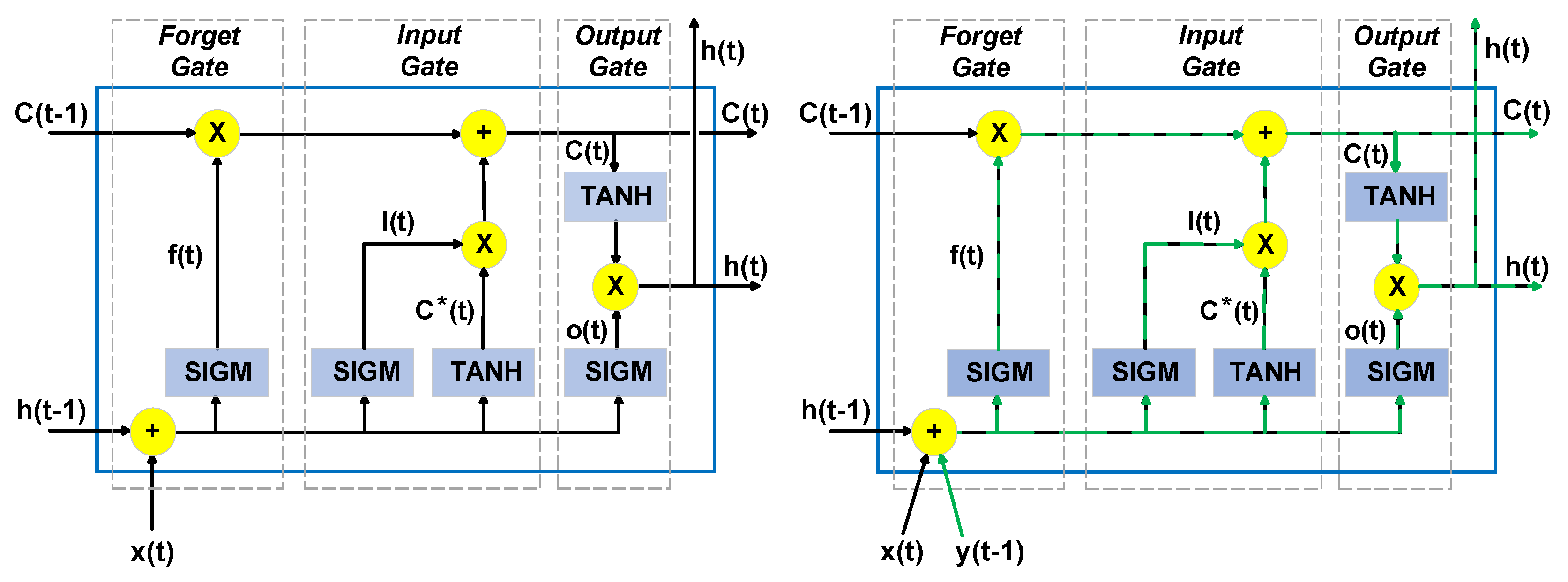
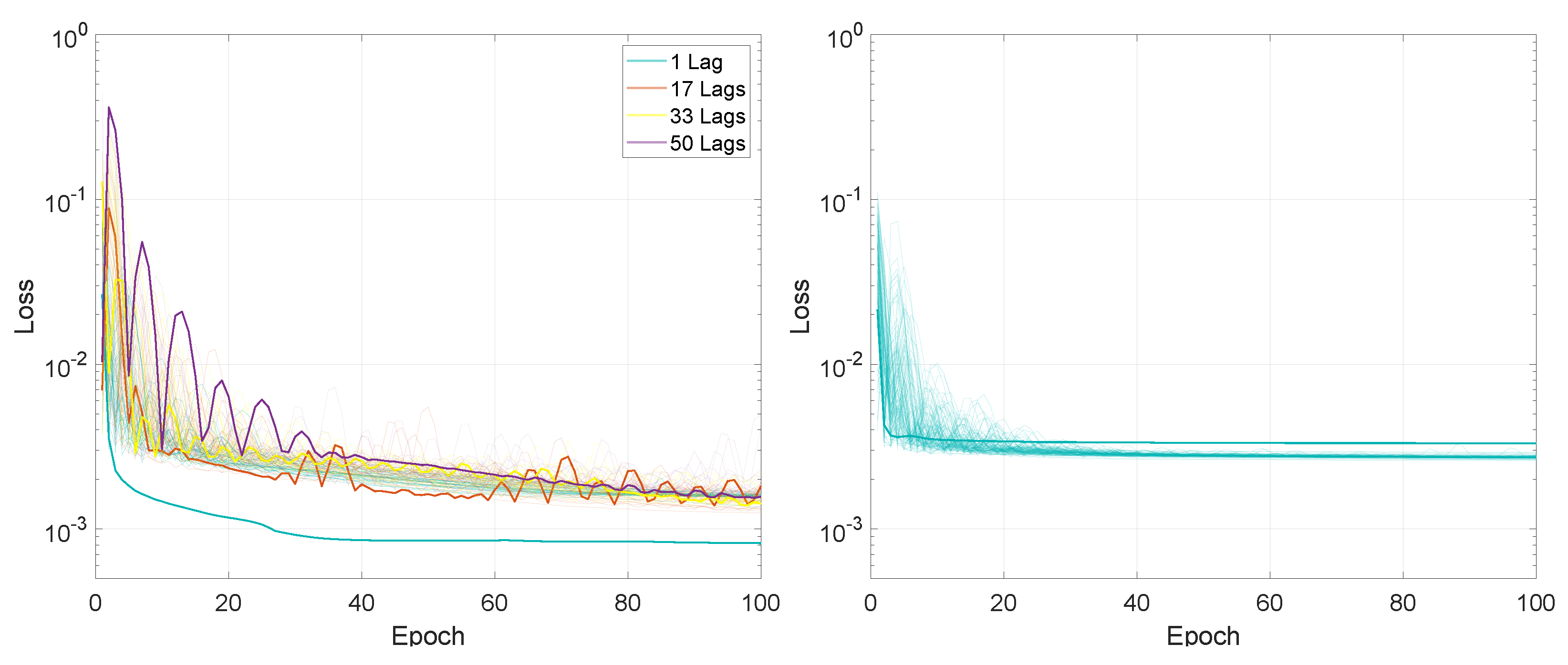
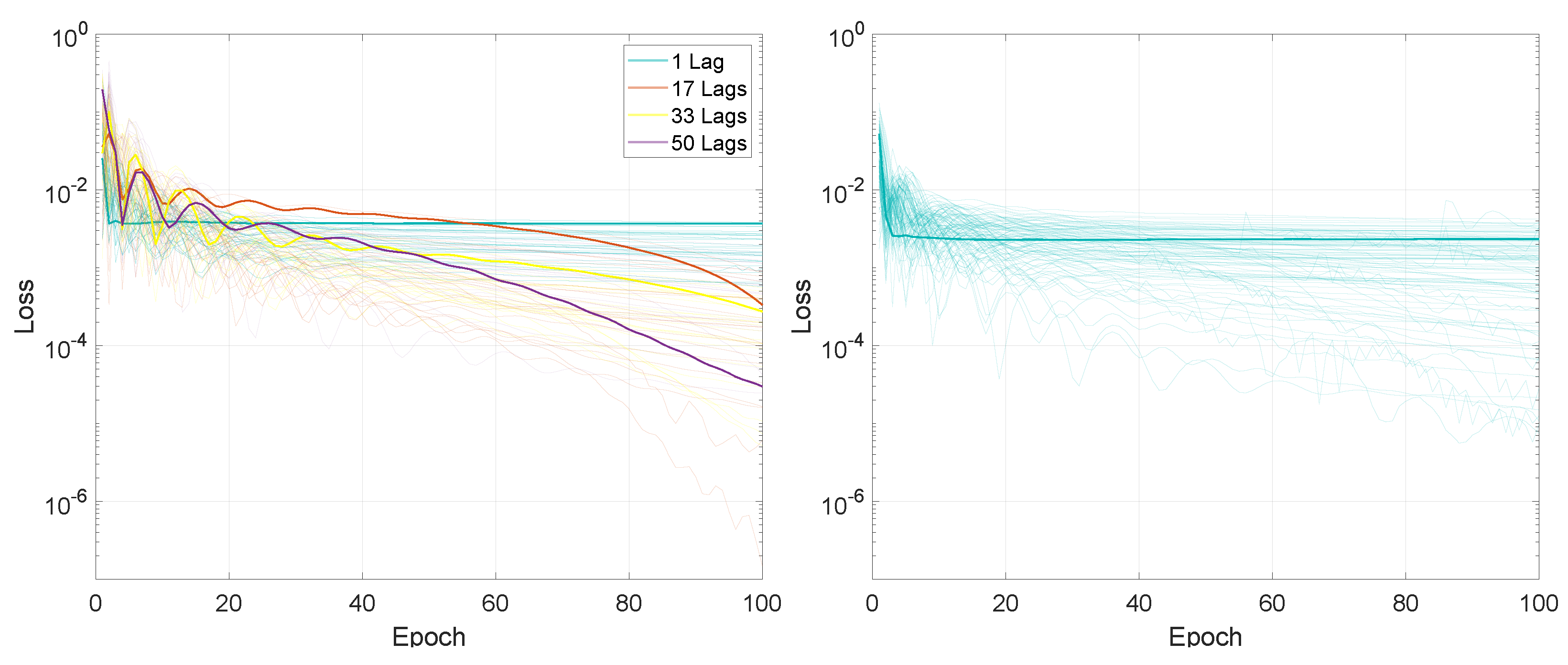
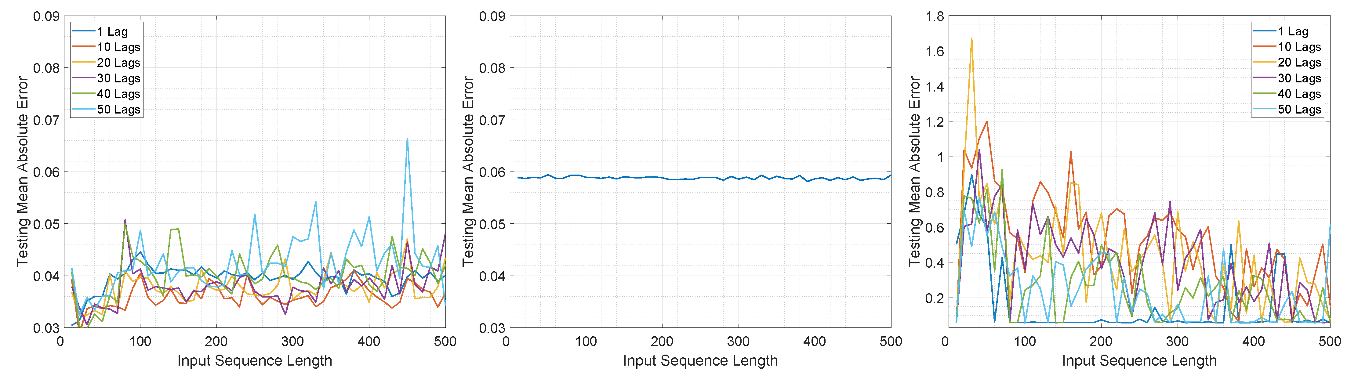
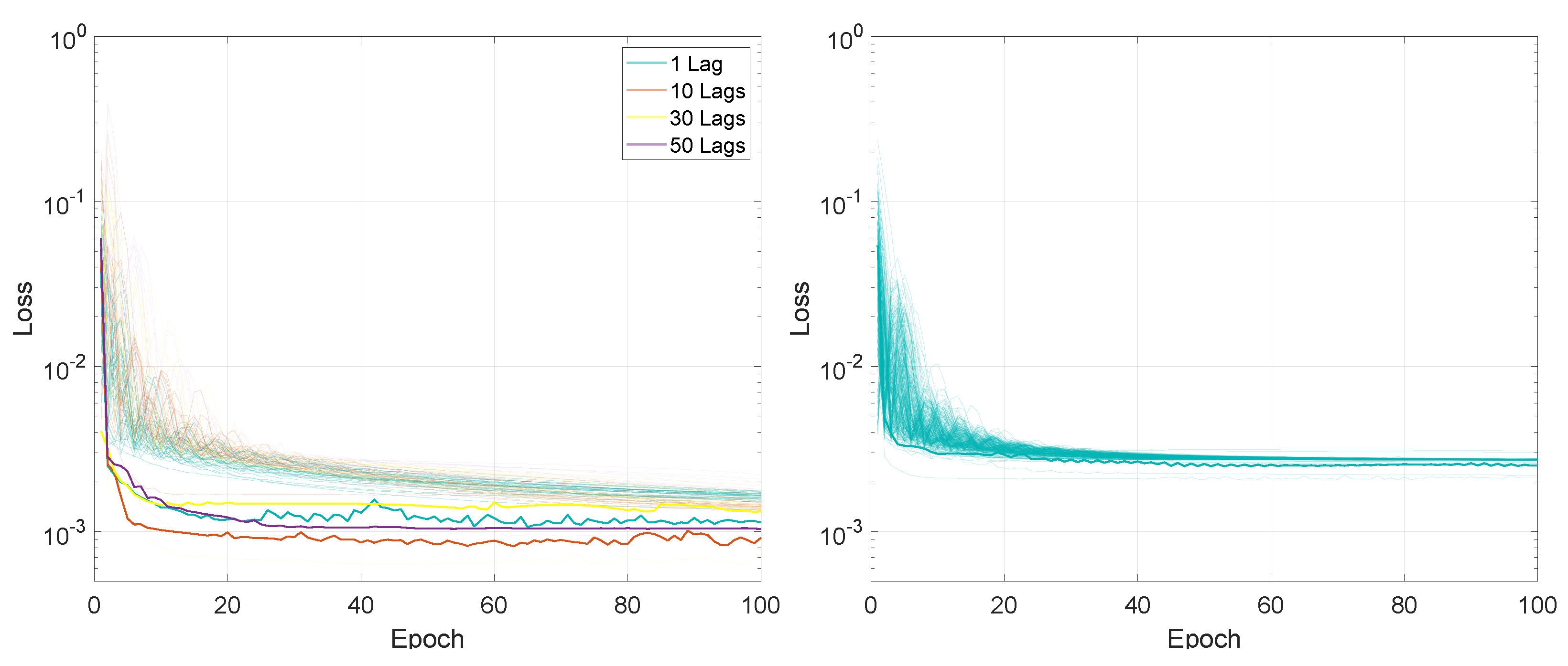
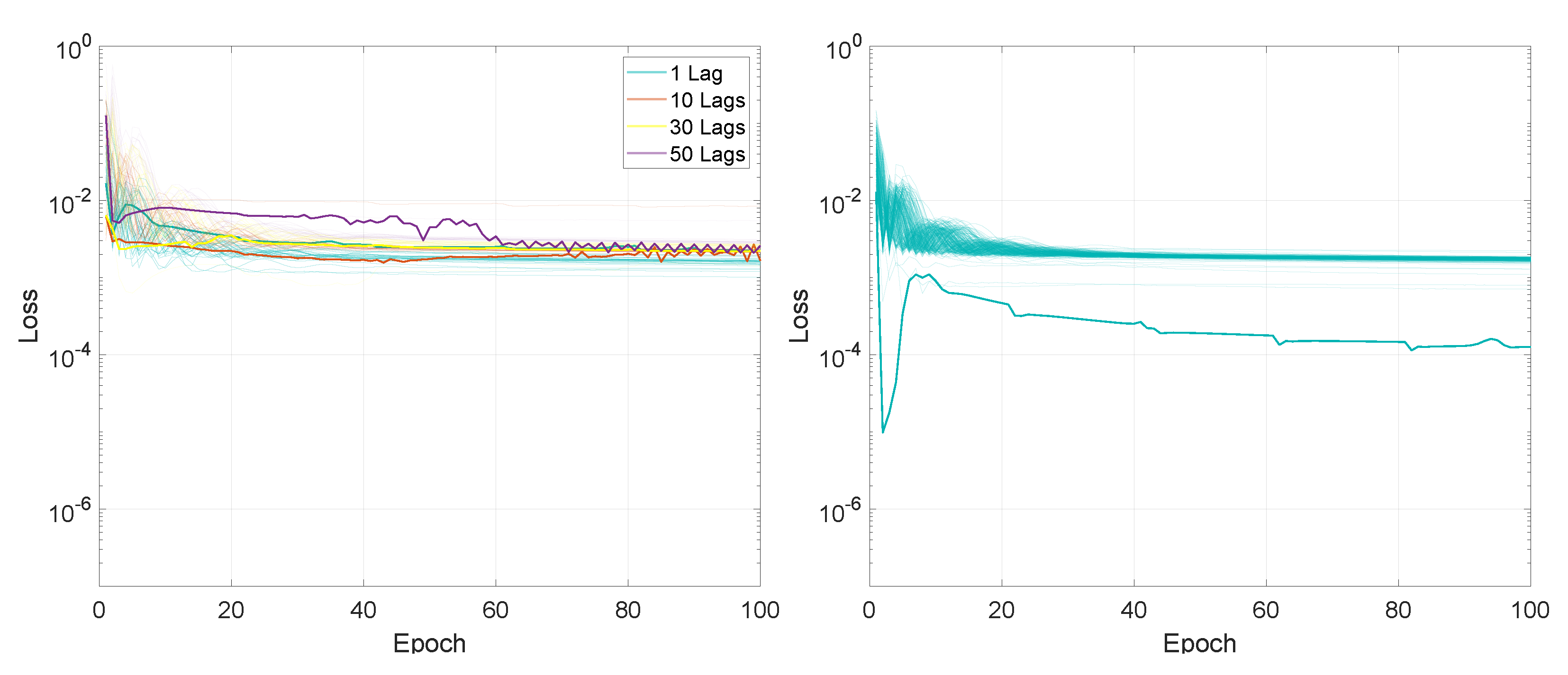
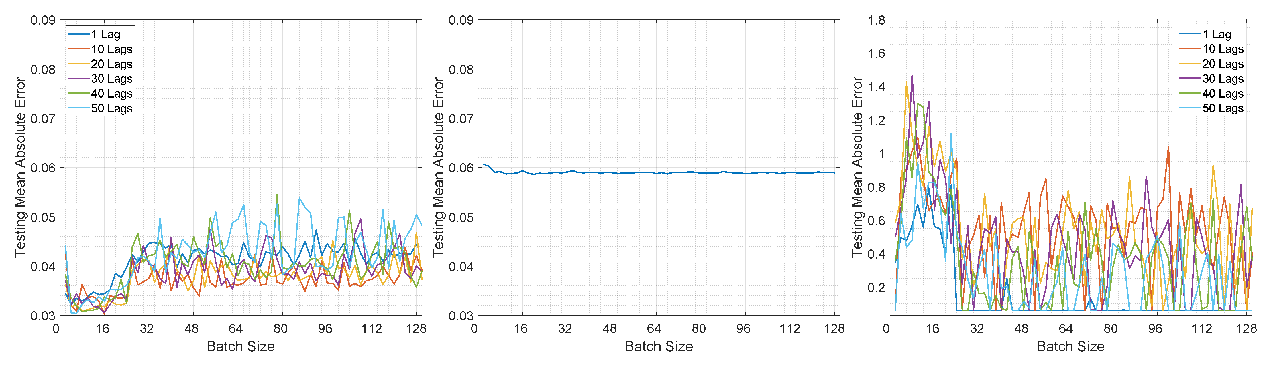
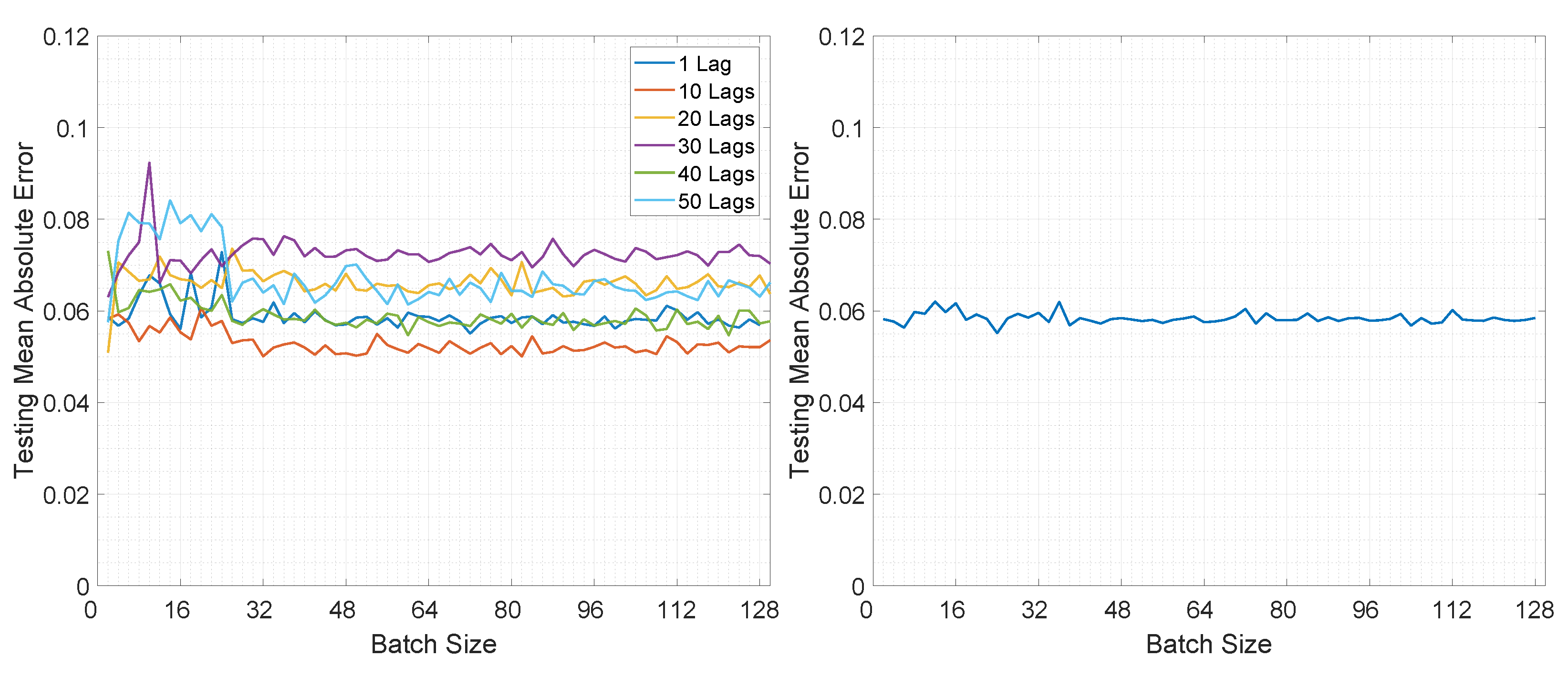
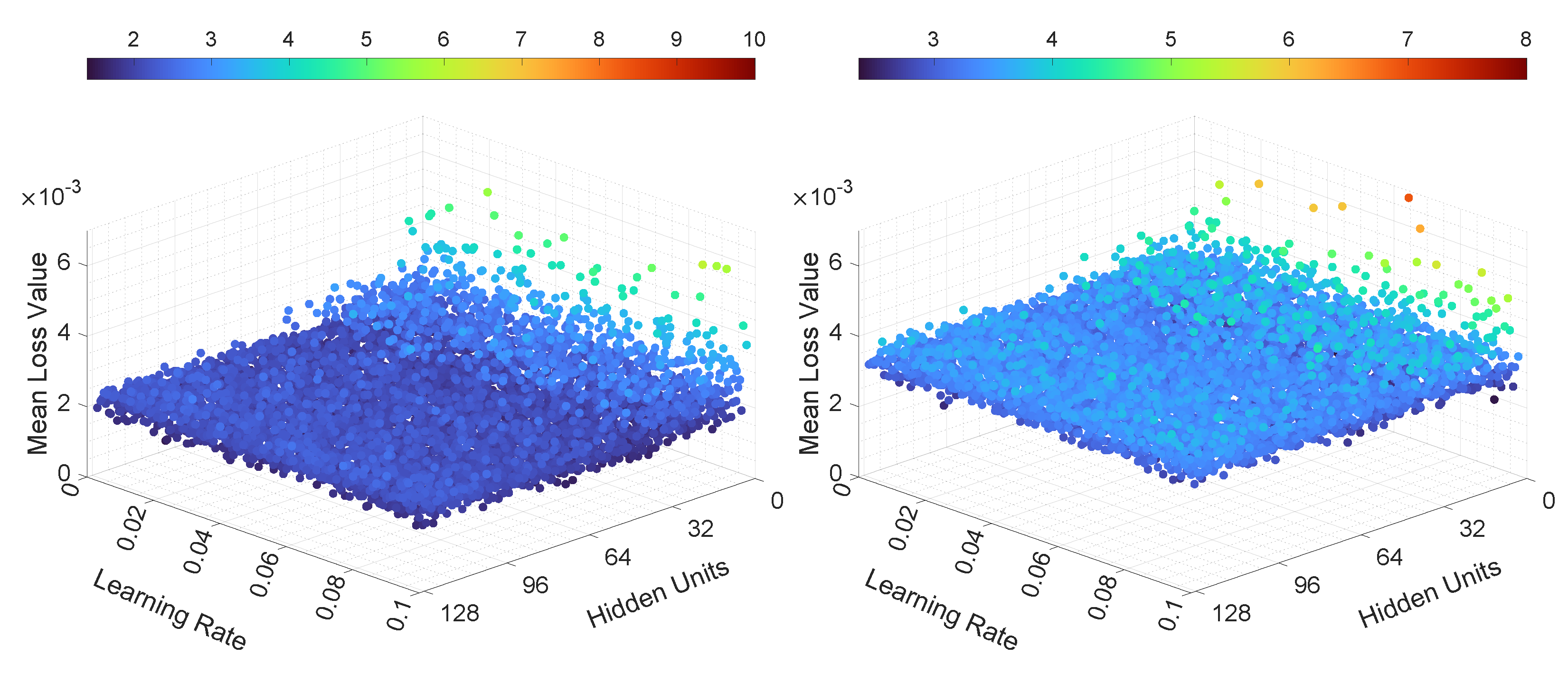
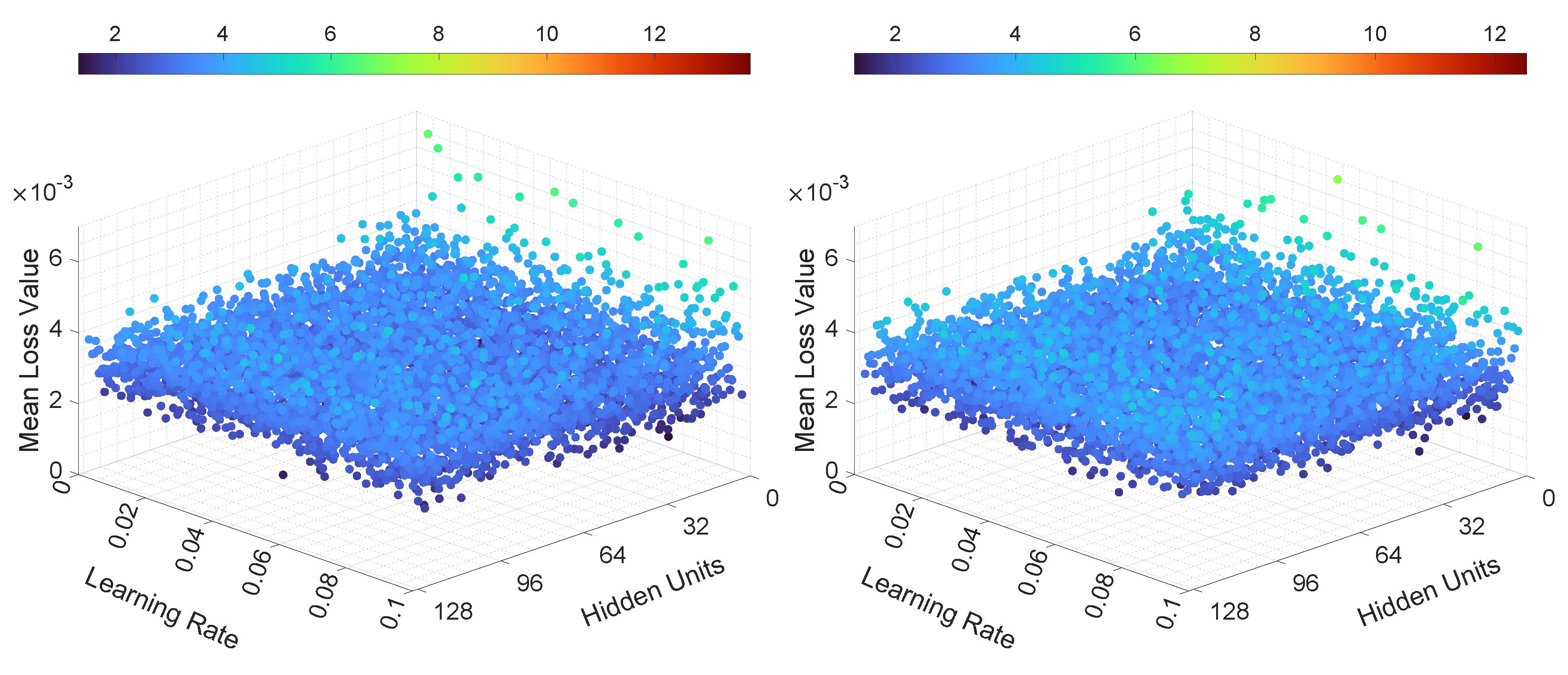
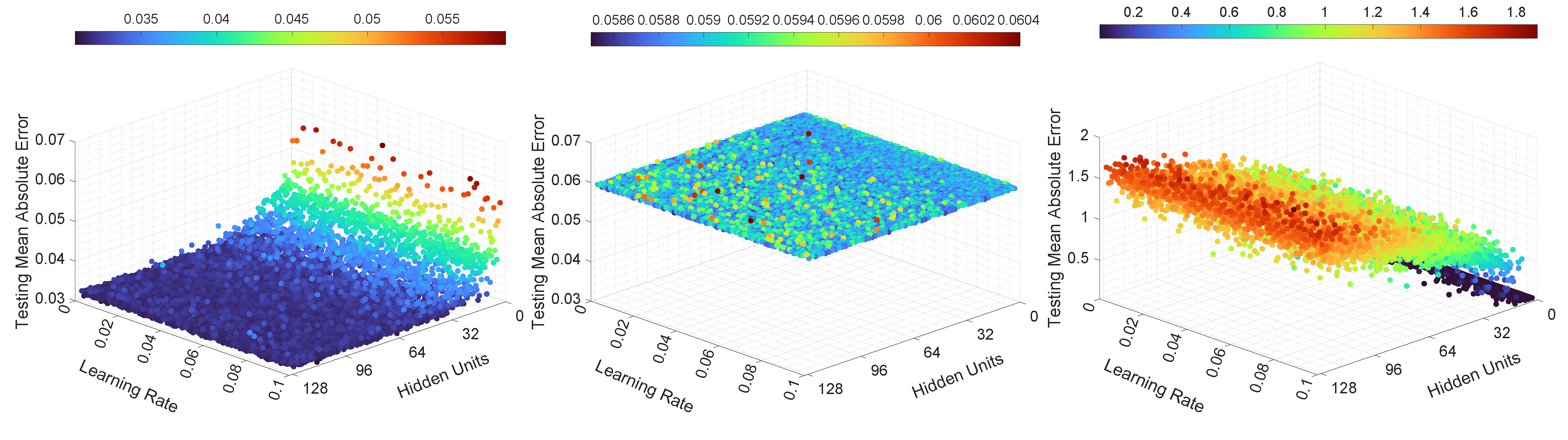
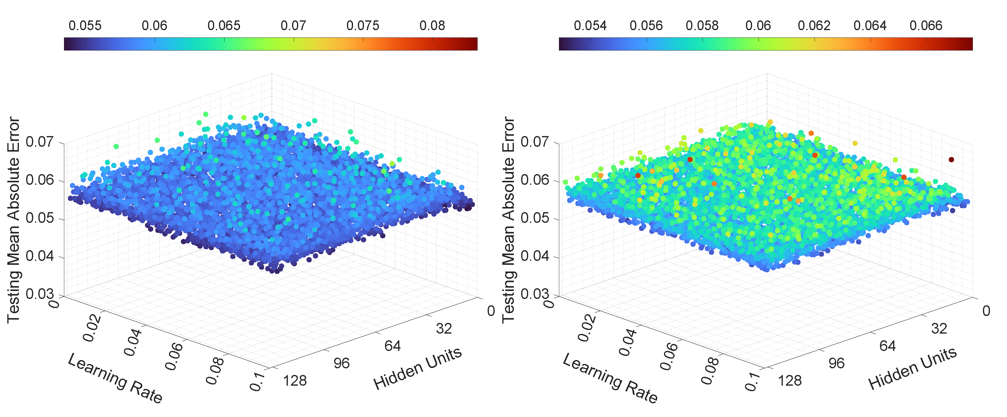
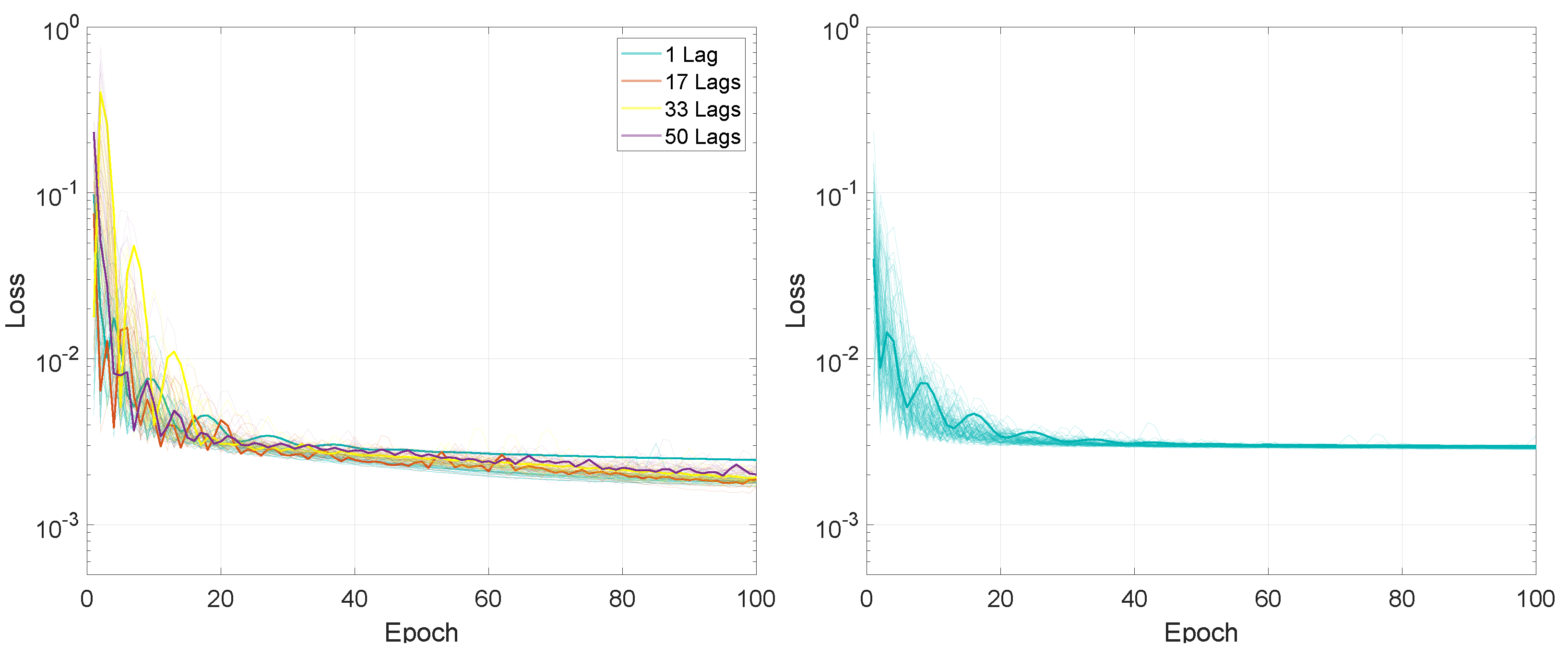
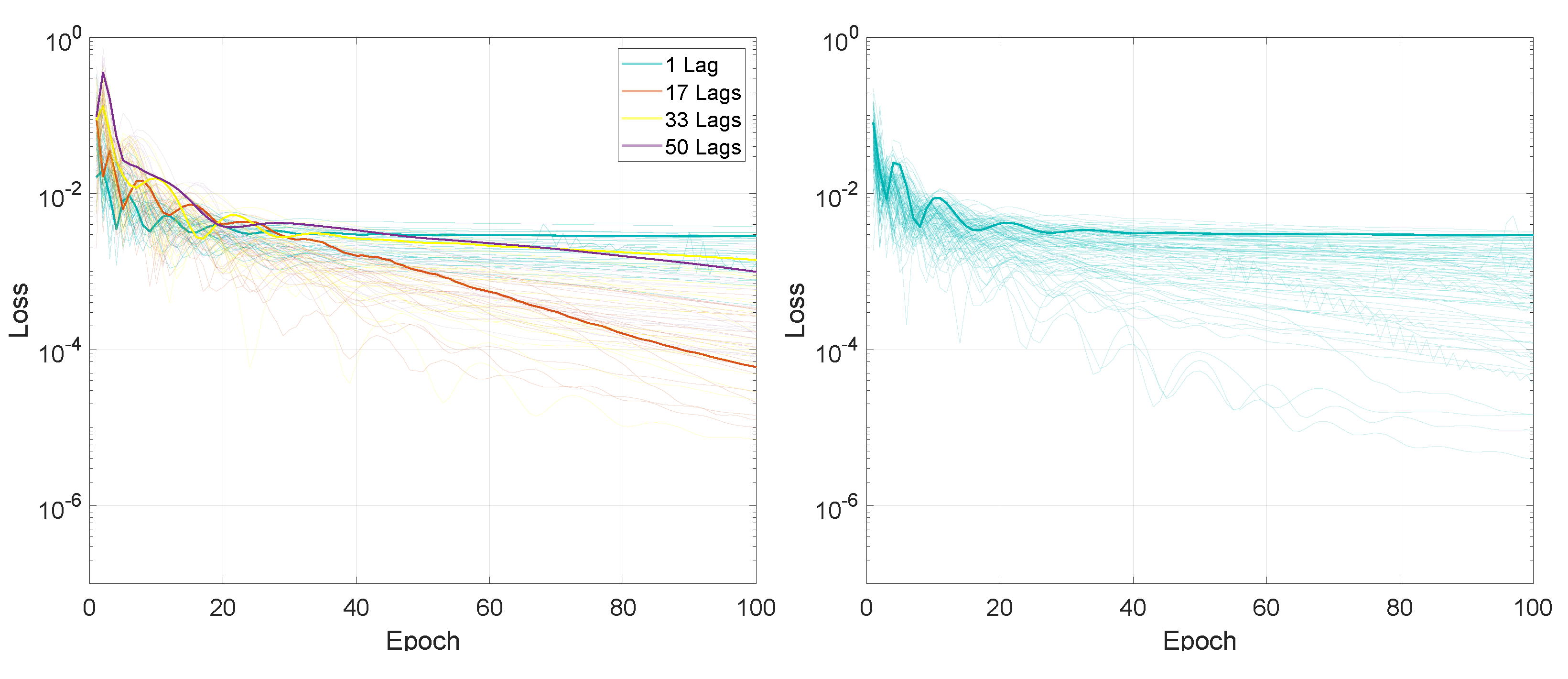
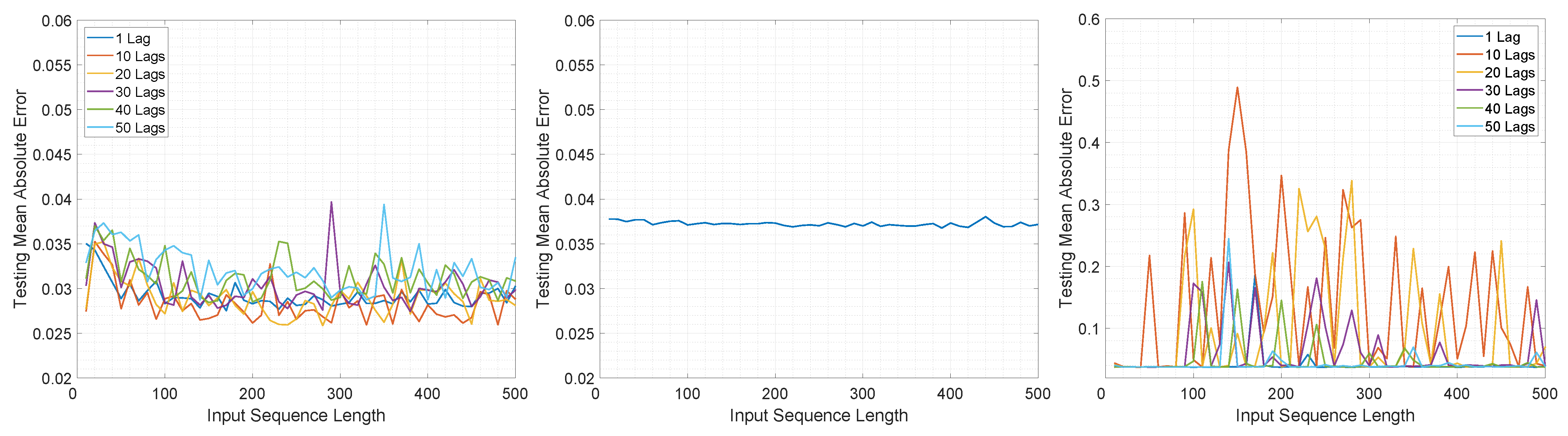
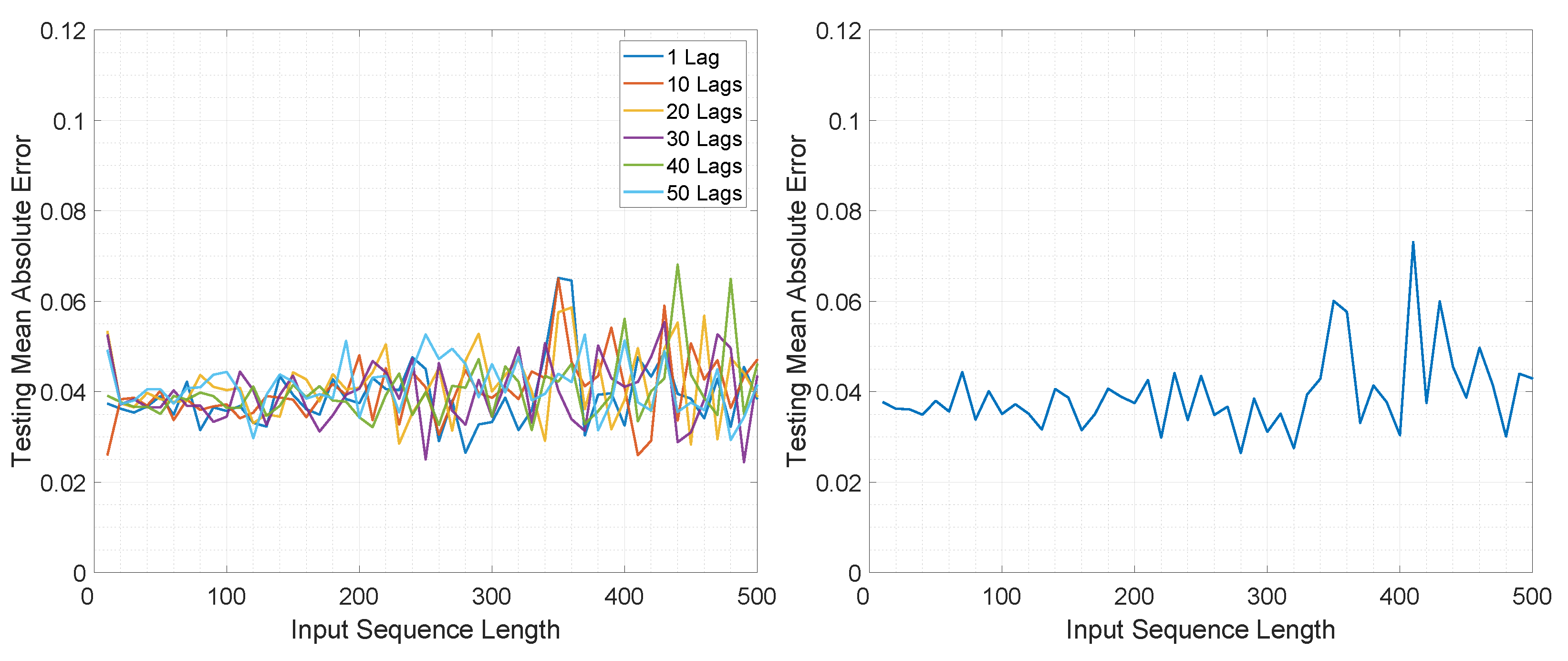
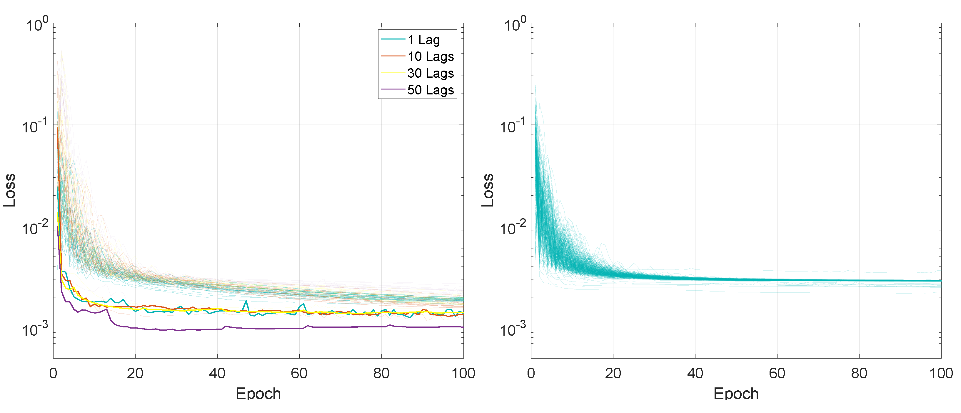
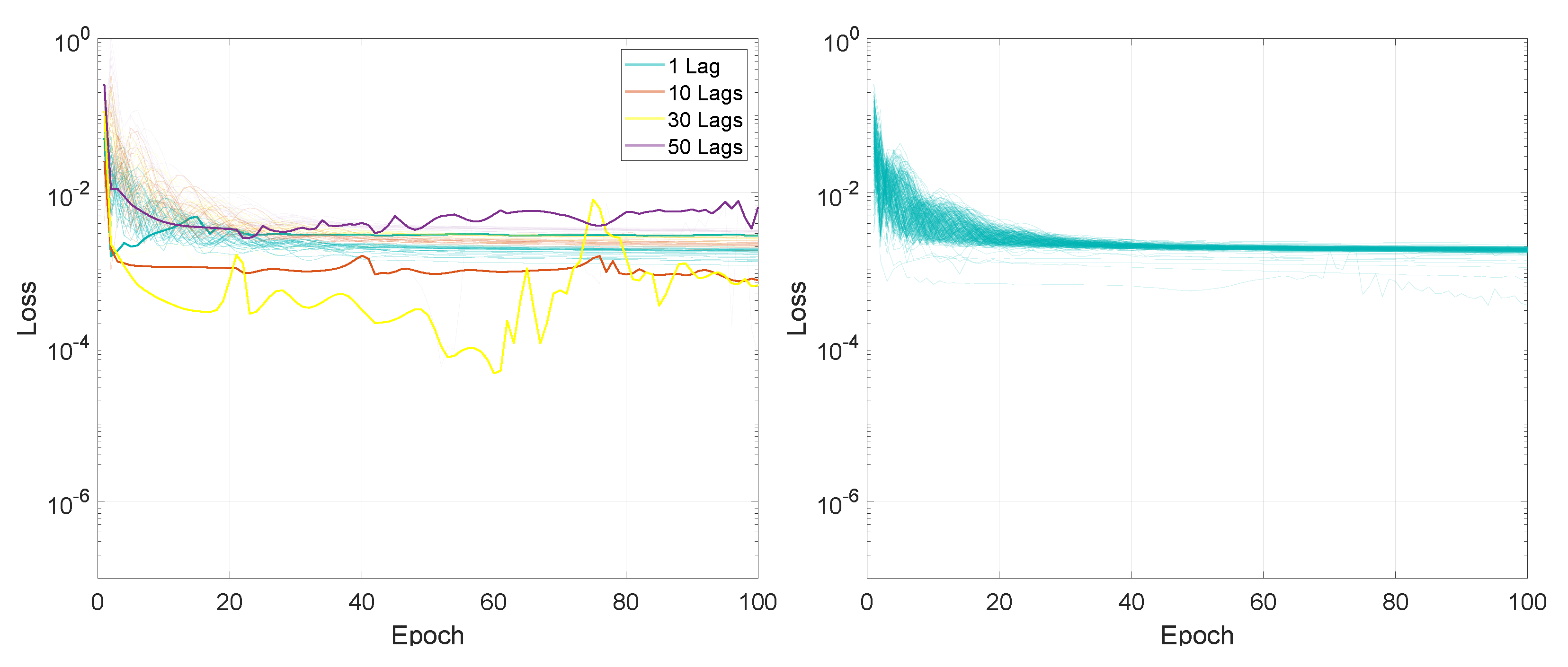
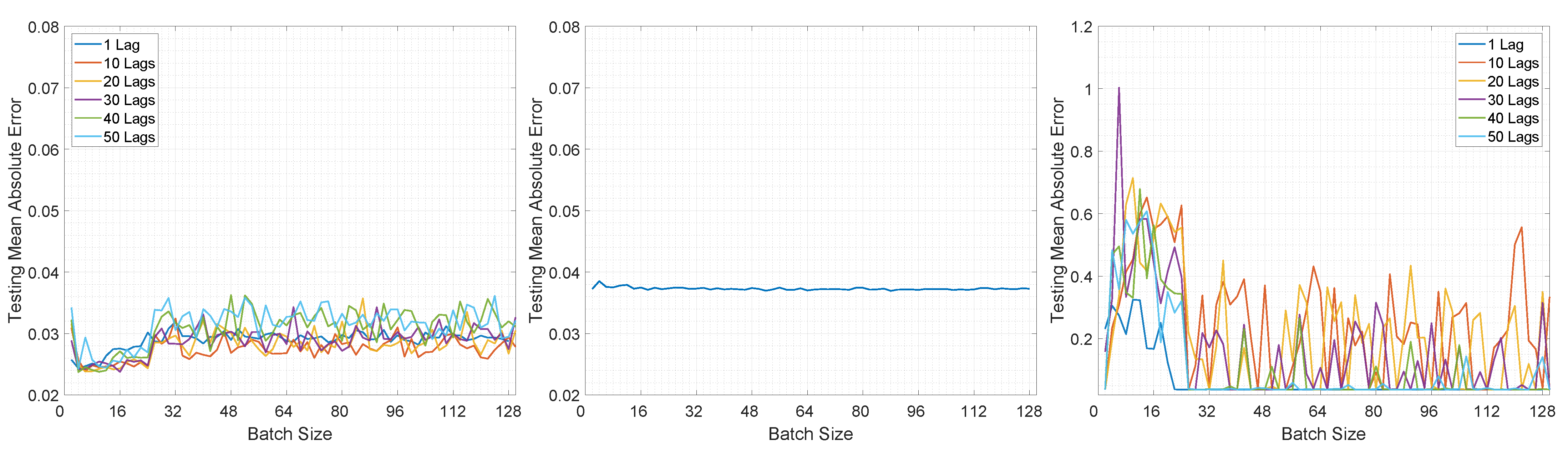
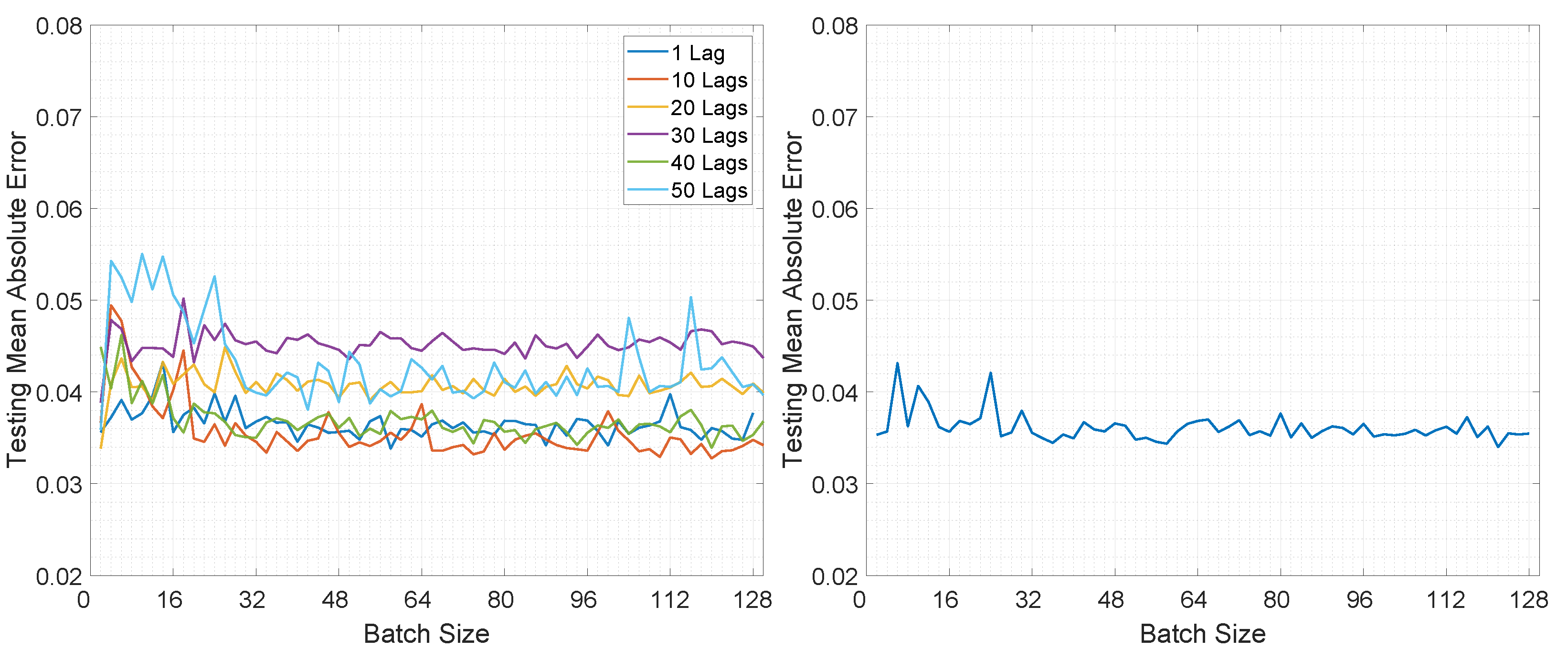
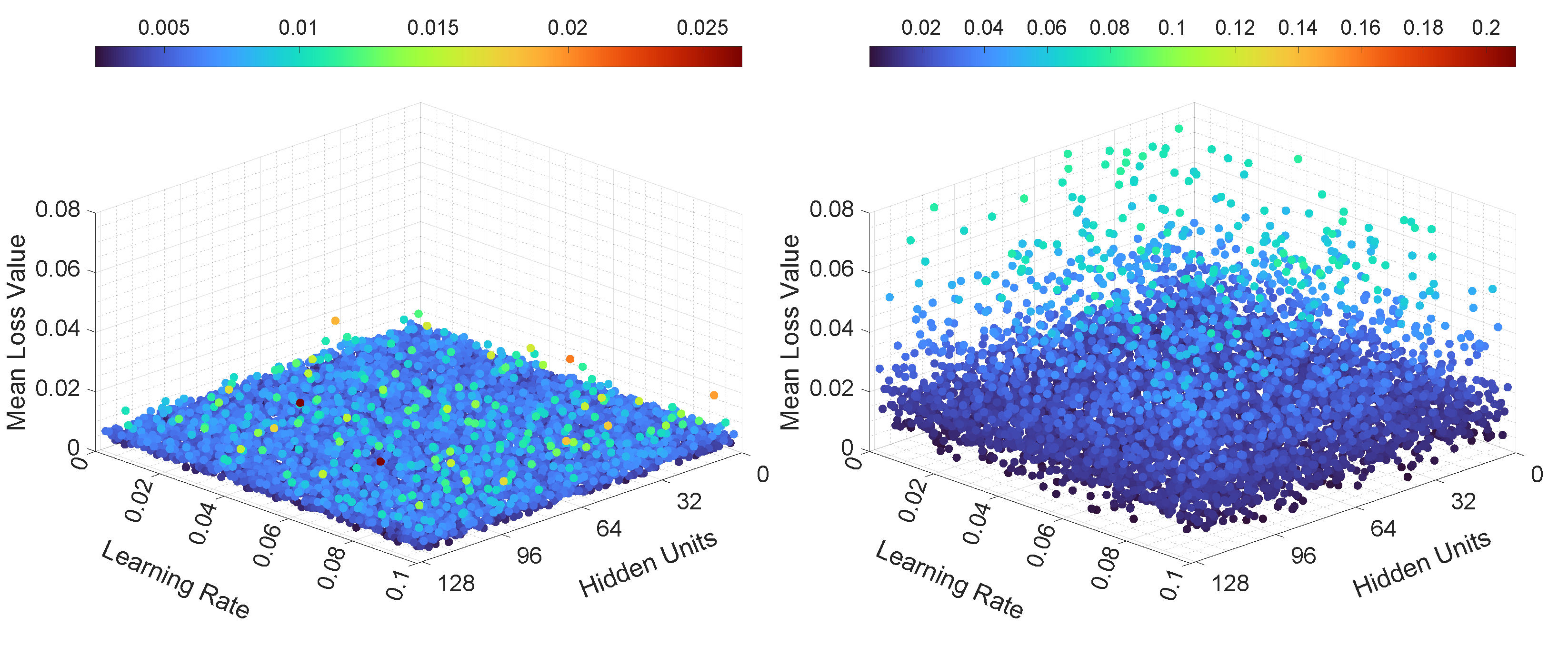
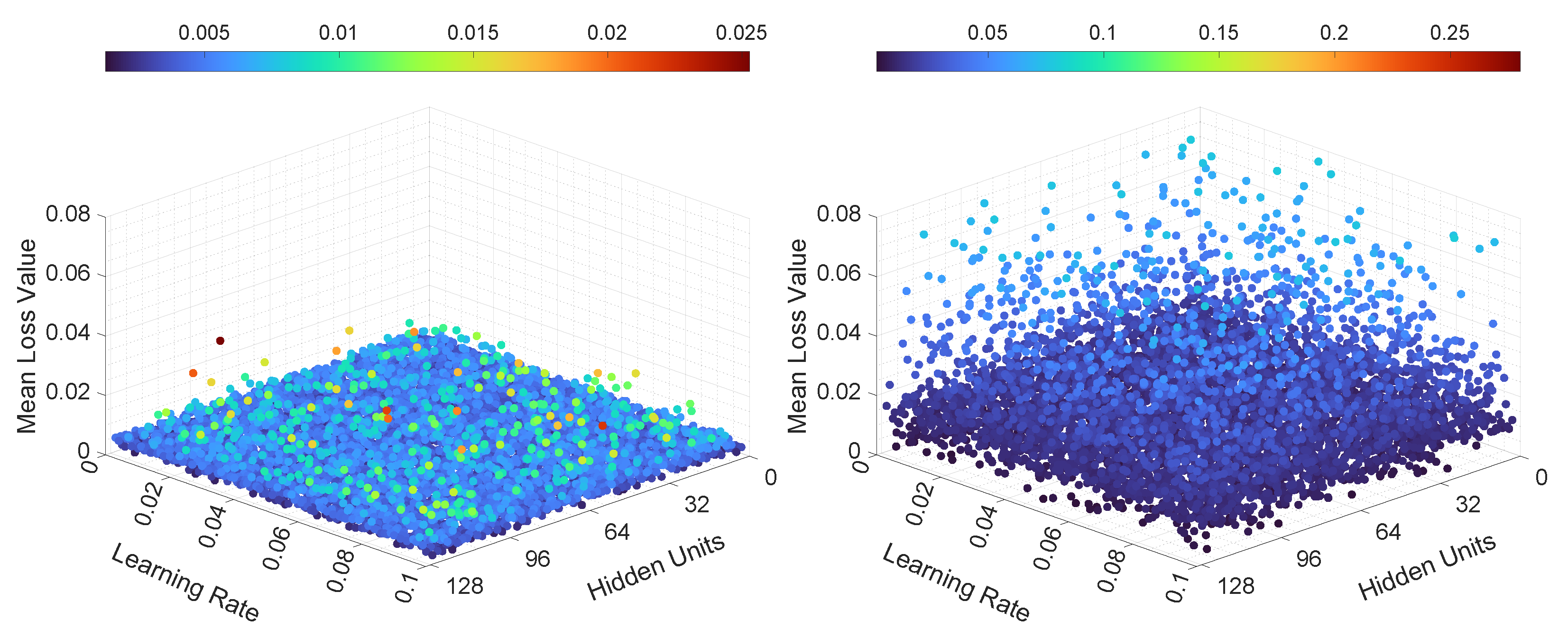
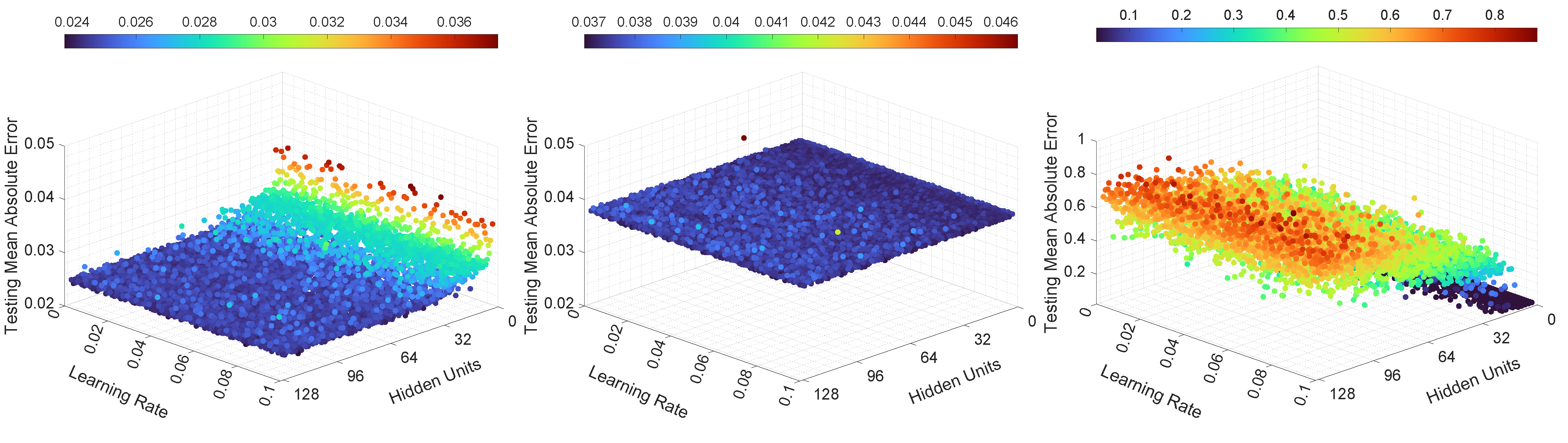
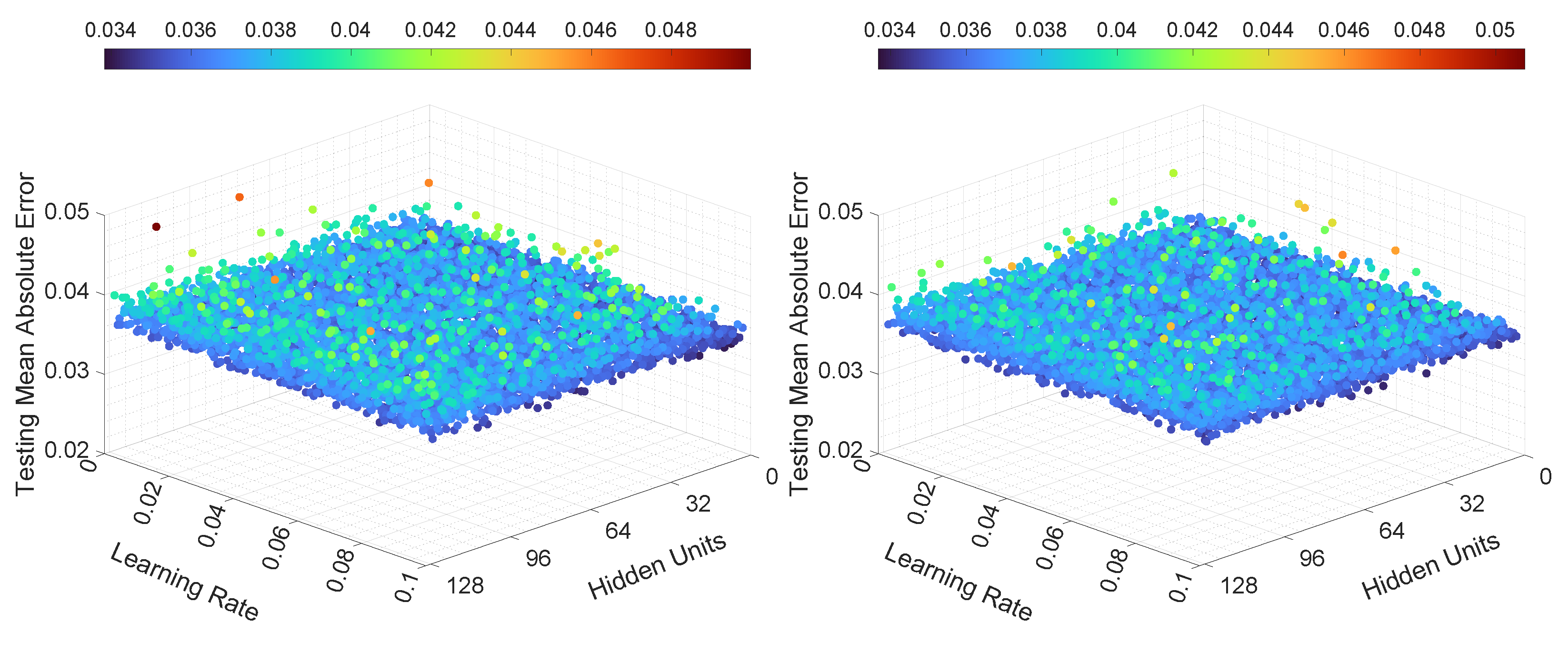
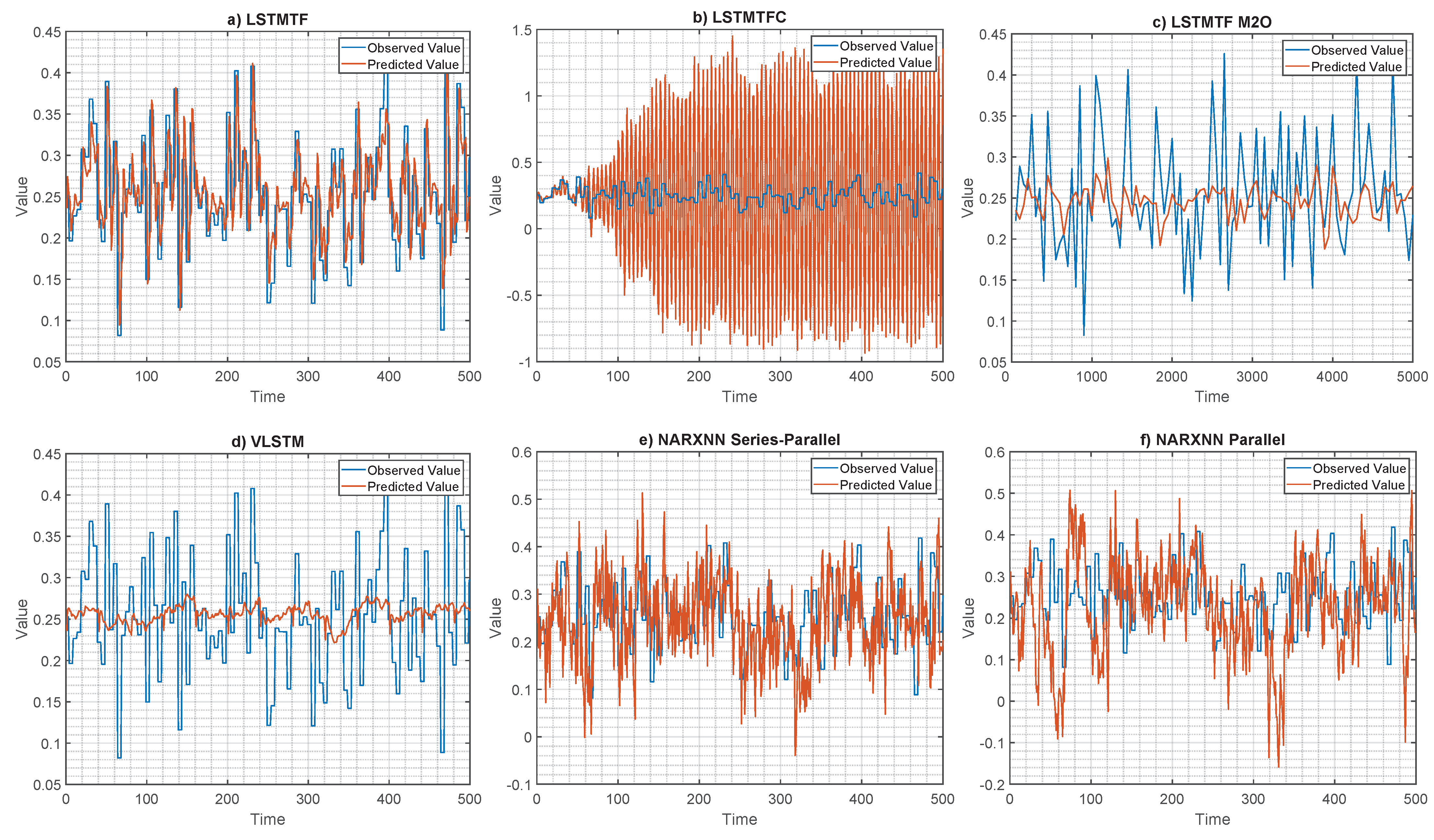
Table 1.
The list of selected inputs and outputs for the MISO and MIMO configurations. A detailed description of the variables can be found in the original TEP paper [42,43].
| Configuration | Output Variables | Input Variables |
|---|---|---|
| MISO | Product Analysis F (Stream 11) | A Feed (stream 1) |
| A and C Feed (Stream 4) | ||
| Product Separator Pressure | ||
| Stripper Pressure | ||
| Stripper Temperature | ||
| Stripper Steam Flow | ||
| Reactor Cooling Water Outlet Temperature | ||
| Reactor feed Analysis B | ||
| Reactor feed Analysis E | ||
| A feed flow (Stream 1) | ||
| Reactor Cooling Water Flow | ||
| MIMO | Product Analysis F (Stream 11) Purge gas analysis (Stream 9) | All Continuous Process Measurements |
| All Process Manipulated Variables |
Table 2.
The complete list of fixed and varying hyperparameter values for Experiments 1–3 for all the tested neural network architectures.
Table 2.
The complete list of fixed and varying hyperparameter values for Experiments 1–3 for all the tested neural network architectures.
| Experiment | Hidden Layers | Sequence Input Length | Hidden Units | Learning Rate | Mini-Batch Size | Epochs | Lags |
|---|---|---|---|---|---|---|---|
| 1 | 1 | [10, 500] | 16 | 0.01 | 32 | 100 | [1, 50] |
| 2 | 1 | 40 | 16 | 0.01 | [1, 128] | 100 | 1 |
| 3 | 1 | 40 | [1, 128] | [0.00001, 0.1] | 32 | 100 | 1 |
Table 3.
The training convergence time (epochs) for LSTMTF, computed with respect to the number of lags, for = 1% and P = 5.
Table 3.
The training convergence time (epochs) for LSTMTF, computed with respect to the number of lags, for = 1% and P = 5.
| Many-to-Many | Many-to-One | |||||
|---|---|---|---|---|---|---|
| Min | Avg | Max | Min | Avg | Max | |
| 1 Lag | 41 | 86 | 100 | 16 | 65 | 100 |
| 10 Lags | 26 | 91 | 100 | 16 | 72 | 100 |
| 20 Lags | 46 | 95 | 100 | 21 | 73 | 100 |
| 30 Lags | 46 | 95 | 100 | 21 | 73 | 100 |
| 40 Lags | 46 | 96 | 100 | 26 | 71 | 100 |
| 50 Lags | 46 | 97 | 100 | 41 | 87 | 100 |
Table 4.
The average training convergence time (epochs) for LSTMTF and VLSTM, computed with respect to the input sequence length, for = 1%, P = 5, and 1 lag for LSTMTF.
Table 4.
The average training convergence time (epochs) for LSTMTF and VLSTM, computed with respect to the input sequence length, for = 1%, P = 5, and 1 lag for LSTMTF.
| LSTMTF | VLSTM | |||
|---|---|---|---|---|
| ISL | Many-to-Many | Many-to-One | Many-to-Many | Many-to-One |
| [10, 100] | 70 | 83 | 32 | 38 |
| [100, 200] | 73 | 69 | 36 | 51 |
| [200, 300] | 86 | 82 | 44 | 57 |
| [300, 400] | 93 | 82 | 66 | 74 |
| [400, 500] | 90 | 86 | 80 | 79 |
Table 5.
The training convergence time (epochs) for LSTMTF and VLSTM, computed with respect to the mini-batch size, for = 1% and P = 5.
Table 5.
The training convergence time (epochs) for LSTMTF and VLSTM, computed with respect to the mini-batch size, for = 1% and P = 5.
| LSTMTF | VLSTM | |||
|---|---|---|---|---|
| MBS | Many-to-Many | Many-to-One | Many-to-Many | Many-to-One |
| 2 | 100 | 46 | 12 | 66 |
| 8 | 51 | 31 | 16 | 41 |
| 16 | 86 | 41 | 41 | 32 |
| 32 | 100 | 51 | 46 | 56 |
| 64 | 86 | 56 | 51 | 56 |
| 128 | 100 | 56 | 51 | 57 |
Table 6.
The training convergence time (epochs) for LSTMTF and VLSTM, computed with respect to the number of hidden units, for = 1% and P = 5.
Table 6.
The training convergence time (epochs) for LSTMTF and VLSTM, computed with respect to the number of hidden units, for = 1% and P = 5.
| LSTMTF | VLSTM | |||
|---|---|---|---|---|
| HU | Many-to-Many | Many-to-One | Many-to-Many | Many-to-One |
| 2 | 81 | 38 | 30 | 38 |
| 8 | 73 | 40 | 25 | 44 |
| 16 | 76 | 43 | 24 | 43 |
| 32 | 79 | 47 | 22 | 44 |
| 64 | 77 | 44 | 22 | 42 |
| 128 | 58 | 47 | 23 | 47 |
Table 7.
The training convergence time (epochs) for LSTMTF and VLSTM, computed with respect to the learning rate, for = 1% and P = 5.
Table 7.
The training convergence time (epochs) for LSTMTF and VLSTM, computed with respect to the learning rate, for = 1% and P = 5.
| LSTMTF | VLSTM | |||
|---|---|---|---|---|
| LR | Many-to-Many | Many-to-One | Many-to-Many | Many-to-One |
| [0.0001, 0.02] | 71 | 46 | 23 | 45 |
| [0.02, 0.04] | 71 | 44 | 23 | 44 |
| [0.04, 0.06] | 71 | 44 | 23 | 44 |
| [0.06, 0.08] | 71 | 45 | 23 | 45 |
| [0.08, 0.1] | 71 | 44 | 23 | 44 |
Table 8.
The actual training and testing times for 50,000 data points, measured in milliseconds, for LSTMTF and VLSTM.
Table 8.
The actual training and testing times for 50,000 data points, measured in milliseconds, for LSTMTF and VLSTM.
| LSTMTF | VLSTM | |||
|---|---|---|---|---|
| Time [ms] | Many-to-Many | Many-to-One | Many-to-Many | Many-to-One |
| MISO Training | 1820 | 1831 | 1810 | 1870 |
| MISO Testing | 46.55 | 49.70 | 47.13 | 45.72 |
| MIMO Training | 2209 | 2294 | 2208 | 2236 |
| MIMO Testing | 57.27 | 63.08 | 60.74 | 61.71 |
Disclaimer/Publisher’s Note: The statements, opinions and data contained in all publications are solely those of the individual author(s) and contributor(s) and not of MDPI and/or the editor(s). MDPI and/or the editor(s) disclaim responsibility for any injury to people or property resulting from any ideas, methods, instructions or products referred to in the content. |
© 2023 by the authors. Licensee MDPI, Basel, Switzerland. This article is an open access article distributed under the terms and conditions of the Creative Commons Attribution (CC BY) license (https://creativecommons.org/licenses/by/4.0/).
Share and Cite
MDPI and ACS Style
Bolboacă, R.; Haller, P. Performance Analysis of Long Short-Term Memory Predictive Neural Networks on Time Series Data. Mathematics 2023, 11, 1432. https://0-doi-org.brum.beds.ac.uk/10.3390/math11061432
AMA Style
Bolboacă R, Haller P. Performance Analysis of Long Short-Term Memory Predictive Neural Networks on Time Series Data. Mathematics. 2023; 11(6):1432. https://0-doi-org.brum.beds.ac.uk/10.3390/math11061432
Chicago/Turabian StyleBolboacă, Roland, and Piroska Haller. 2023. "Performance Analysis of Long Short-Term Memory Predictive Neural Networks on Time Series Data" Mathematics 11, no. 6: 1432. https://0-doi-org.brum.beds.ac.uk/10.3390/math11061432
Note that from the first issue of 2016, this journal uses article numbers instead of page numbers. See further details here.