
Hybrid Newton–Sperm Swarm Optimization Algorithm for Nonlinear Systems
by
 , , , and
Obadah Said Solaiman
1,
Rami Sihwail
2,*,
Hisham Shehadeh
3,
Ishak Hashim
1,4 and
Kamal Alieyan
2 1
Department of Mathematical Sciences, Faculty of Science & Technology, Universiti Kebangsaan Malaysia, Bangi 43600, Selangor, Malaysia
2
Department of Cyber Security, Faculty of Computer Science & Informatics, Amman Arab University, Amman 11953, Jordan
3
Department of Computer Information System, Faculty of Computer Science & Informatics, Amman Arab University, Amman 11953, Jordan
4
Nonlinear Dynamics Research Center (NDRC), Ajman University, Ajman P.O. Box 346, United Arab Emirates
*
Author to whom correspondence should be addressed.
Mathematics 2023, 11(6), 1473; https://0-doi-org.brum.beds.ac.uk/10.3390/math11061473
Submission received: 6 February 2023
/
Revised: 11 March 2023
/
Accepted: 14 March 2023
/
Published: 17 March 2023
(This article belongs to the Special Issue Numerical Methods for Solving Nonlinear Equations)
Abstract
:Several problems have been solved by nonlinear equation systems (NESs), including real-life issues in chemistry and neurophysiology. However, the accuracy of solutions is highly dependent on the efficiency of the algorithm used. In this paper, a Modified Sperm Swarm Optimization Algorithm called MSSO is introduced to solve NESs. MSSO combines Newton’s second-order iterative method with the Sperm Swarm Optimization Algorithm (SSO). Through this combination, MSSO’s search mechanism is improved, its convergence rate is accelerated, local optima are avoided, and more accurate solutions are provided. The method overcomes several drawbacks of Newton’s method, such as the initial points’ selection, falling into the trap of local optima, and divergence. In this study, MSSO was evaluated using eight NES benchmarks that are commonly used in the literature, three of which are from real-life applications. Furthermore, MSSO was compared with several well-known optimization algorithms, including the original SSO, Harris Hawk Optimization (HHO), Butterfly Optimization Algorithm (BOA), Ant Lion Optimizer (ALO), Particle Swarm Optimization (PSO), and Equilibrium Optimization (EO). According to the results, MSSO outperformed the compared algorithms across all selected benchmark systems in four aspects: stability, fitness values, best solutions, and convergence speed.
Keywords:
nonlinear systems; Newton’s method; iterative methods; sperm swarm optimization algorithm; optimization algorithmMSC:
65D99; 65H10; 65K101. Introduction
Many issues in the natural and applied sciences are represented by systems of nonlinear equations that require solving, where such that is nonlinear for all . It is well known that determining the precise solution to the nonlinear system is a difficult undertaking, especially when the equation comprises terms made up of logarithmic, exponential, trigonometric, or a mix of any transcendental terms. Thus, finding approximate solutions to this type of problem has emerged as a need. The iterative methods, including Newton’s method, are some of the most famous methods for finding approximate solutions to nonlinear equation systems (NESs) [1]. Alternatively, optimization algorithms have been applied in attempts to extract the root solution of nonlinear systems.
In the last ten years, various optimization algorithms have been developed. Those methods can be divided into four primary categories: human-based methods, swarm-based methods, physical-based methods, and evolutionary-based methods [2]. Human perception, attitude, or lifestyle influence human-based methods. Examples of these methods are the “Harmony Search Algorithm (HSA)” [3] and the “Fireworks Algorithm (FA)” [4]. Swarm-based methods mimic the behavior of swarms or animals to reproduce or survive. Examples of this algorithm are “Sperm Swarm Optimization (SSO)” [5,6,7,8], “Harris Hawks Optimization (HHO)” [9], “The Ant Lion Optimizer (ALO)” [10], and “Butterfly Optimization Algorithm (BOA)” [11]. Some representative swarm intelligence optimization methods and applications have also been proposed; see for example, [12]. Physical-based methods are inspired by both physical theories and the universe’s rules. An example of these algorithms is the “Gravitational Search Algorithm (GSA)” [2], and “Equilibrium Optimizer (EO)” [13]. Evolutionary-based methods are inspired by the Darwinian theory of evolution. An example of this method is the “Genetics Algorithm (GA)” [14]. Finally, some advanced optimization methods with applications from the real-life have been proposed, for example [15,16].
The primary objectives of these methods are to yield the optimal solution and a higher convergence rate. Meta-heuristic optimization should be based on exploration and exploitation concepts to achieve global optimum solutions. The exploitation concept indicates the ability of a method to converge to the optimal potential solution. In contrast, exploration refers to the power of algorithms to search the entire space of a problem domain. Therefore, the main goal of meta-heuristic methods is to balance the two concepts.
However, different meta-heuristic methods have been developed to find solutions to various real-life tasks. The use of optimization algorithms for solving NESs is significant and critical. Various optimization algorithms are used in the solution of nonlinear systems. The following may be summarized:
By improving the performance of optimization algorithms, researchers have been able to target more accurate solutions. For example, Zhou and Li [17] provided a unified solution to nonlinear equations using a modified CSA version. FA was modified by Ariyaratne et al. [18], who made it possible to make the root approximation simultaneously with continuity, differentiation, and initial assumptions. Ren et al. [19] proposed another variation by combining GA with harmonic and symmetric individuals. Chang [20] also revised the GA to estimate better parameters for NESs.
Furthermore, complex systems were handled by Grosan and Abraham [21] by putting them in the form of multi-objective optimization problems. Jaberipour et al. [22] addressed NESs using a modified PSO method; the modification aims to overcome the core PSO’s drawbacks, such as delayed convergence and trapping at local minimums. Further, NESs have been addressed by Mo and Liu [23], who added the “Conjugate Direction Method (CDM)” into the PSO algorithm. The algorithm’s efficiency for solving high-dimensional problems and overcoming local minima was increased by using CDM [24].
Several research methods involved combining two population-based algorithms (PBAs) to achieve more precise results in nonlinear modeling systems. These combinations produce hybrid algorithms that inherit the benefits of both techniques while reducing their downsides [25]. Hybrid ABC [26], hybrid ABC and PSO [27], hybrid FA [28], hybrid GA [29], hybrid KHA [30], hybrid PSO [31], and many others [32,33,34,35,36] are some examples of hybridizing PBAs.
NESs have often been solved using optimization techniques, either using a “Single Optimization Algorithm (SOA)” or a hybrid algorithm that combines two optimization procedures. Only a few researchers have attempted to combine the iterative method and an optimization approach. Karr et al. [37] presented a hybrid method combining Newton’s method and GA for obtaining solutions for nonlinear testbed problems. After using GA to identify the most efficient starting solution, Newton’s approach was utilized. To solve systems of nonlinear models, a hybrid algorithm described by Luo et al. [38] can be utilized; the combination includes GA, Powell algorithm, and Newton’s method. Luo et al. [39] have provided a method for solving NESs by integrating chaos and quasi-Newton techniques. Most of the previous research has concentrated on a specific topic or issue rather than attempting to examine NESs. In a relatively recent study, Sihwail et al. [40] developed a hybrid algorithm known as NHHO to solve arbitrary NESs of equations that combine Harris Hawks’ optimization method and Newton’s method. Very recently, Sihwail et al. [41] proposed a new algorithm for solving NESs of equations in which Jarratt’s iterative approach and the Butterfly optimization algorithm were combined to create the new scheme known as JBOA.
A hybrid algorithm can leverage the benefits of one method while overcoming the drawbacks of the other. However, most hybrid methods face problems with premature convergence due to the technique used in the original algorithms [42]. As a result, choosing a dependable combination of algorithms to produce an efficient hybrid algorithm is a crucial step.
One of the more recent swarm-based methods is Sperm Swarm Optimization (SSO), which is based on the mobility of flocks of sperm to fertilize an ovum. There are various benefits of SSO, which can be listed as follows [2,5,6]:
- The capability of exploitation of SSO is very robust.
- Several kinds of research have validated its simplicity, efficiency, and ability to converge to the optimal solution.
- Its theory can be applied to a wide range of problems in the areas of engineering and science.
- Its mathematical formulation is easy to implement, understand, and utilize.
However, most NESs simulate different data science and engineering problems that have more than one solution. Hence, it is difficult to give accurate solutions to these problems. Like other optimization algorithms, SSO may fall into a local minimum (solution) instead of the optimal solution. As a result, we developed a hybrid approach that incorporates Newton’s iterative scheme with the SSO algorithm to mitigate the drawback. It is worth mentioning that Newton’s method is the first known iterative scheme for solving nonlinear equations using the successive approximation technique. According to Newton’s method, the correct digits nearly double each time a step is performed, referred to as the second order of convergence.
Newton’s method is highly dependent on choosing the correct initial point. To achieve good convergence toward the root, the starting point, like other iterative approaches, must be close enough to the root. The scheme may converge slowly or diverge if the initial point is incorrect. Consequently, Newton’s method can only perform limited local searches in some cases.
For the reasons outlined above, a hybrid SSO algorithm (MSSO) has been proposed to solve NESs, where Newton’s method is applied to improve the search technique and SSO is used to enhance the selection of initial solutions and make global search more efficient.
It is not the concern of this study to demonstrate that hybridizing the SSO and Newton’s methods performs better than other optimization algorithms such as PSO or genetic algorithms. However, this work aims to highlight the benefits of hybridizing an optimization algorithm with an iterative method. This is to enhance the iterative method’s accuracy in solving nonlinear systems and reduce its complexity. Further, it is also able to overcome several drawbacks of Newton’s method, such as initial point selection, trapping in local optima, and divergence problems. Moreover, hybridization in MSSO is beneficial in finding better roots for the selected NSEs. Optimization algorithms alone are unlikely to provide precise solutions compared to iterative methods such as Newton’s method and Jarratt’s method.
The proposed modification improves the initial solution distribution in the search space domain. Moreover, compared to the random distribution used by the original technique, Newton’s approach improves the computational accuracy of SSO and accelerates its convergence rate. Hence, this research paper aims to improve the accuracy of NES solutions. The following are the main contributions of this paper:
- We present a Modified Newton–Sperm Swarm Optimization Algorithm (MSSO) that combines Newton’s method and SSO to enhance its search mechanism and speed up its convergence rate.
- The proposed MSSO method is intended to solve nonlinear systems of different orders.
- Different optimization techniques were compared with MSSO, including the original SSO, PSO, ALO, BOA, HHO, and EO. The comparison was made based on multiple metrics, such as accuracy, fitness value, stability, and convergence speed.
The rest of the paper is organized as follows: Section 2 discusses SSO algorithms and Newton’s iterative method. Section 3 describes the proposed MSSO. Section 4 describes the experiments on the benchmark systems and their results. Further discussion of the findings is provided in Section 5. Finally, Section 6 presents the study’s conclusion.
2. Background
2.1. Standard Sperm Swarm Optimization (SSO) Algorithm
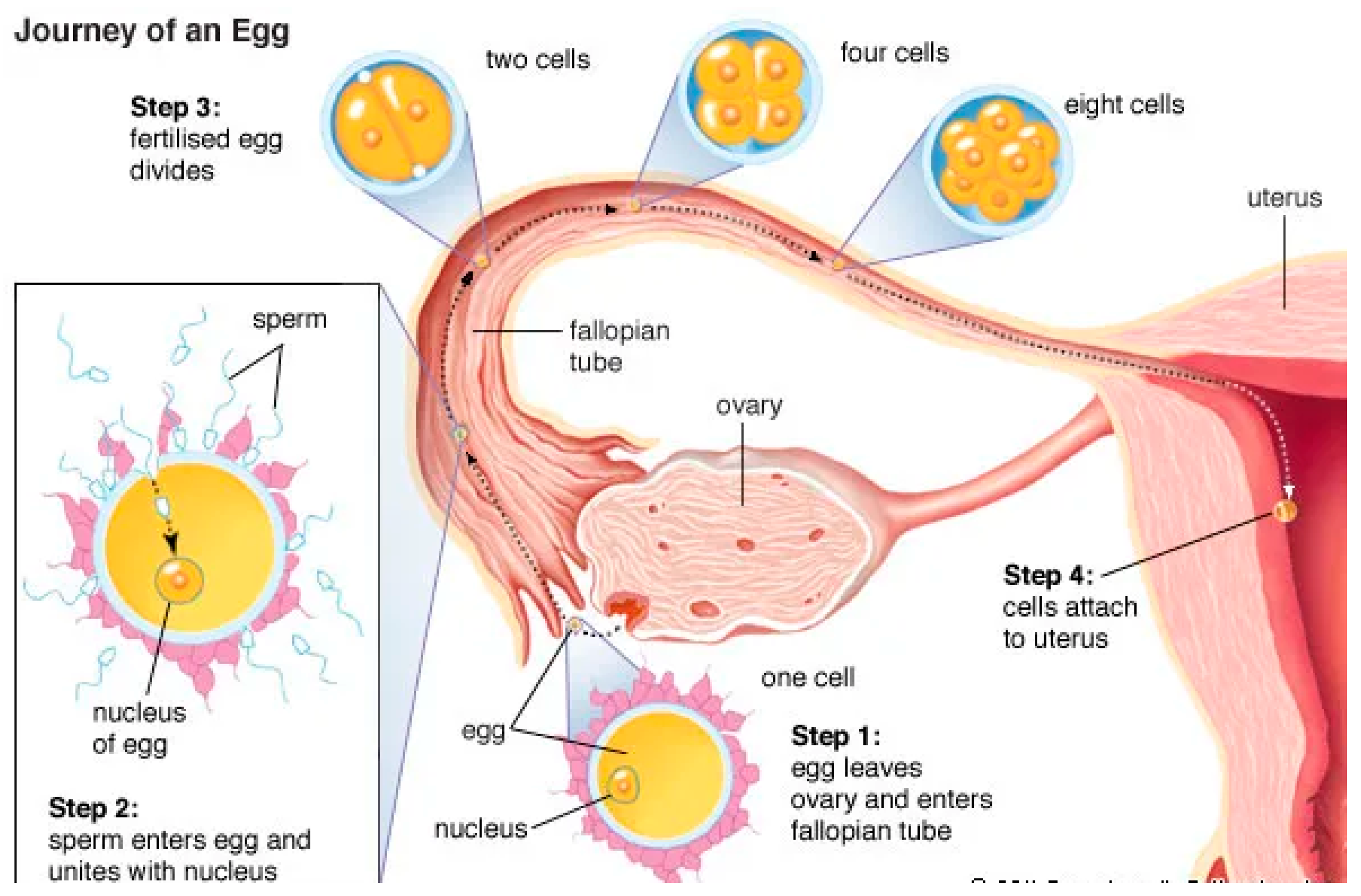
SSO is a newly created swarm-based technique proposed by Shehadeh et al. [2,5,6] that draws inspiration from the actions of a group of sperm as they fertilize an ovum. In the process of fertilization, a single sperm navigates a path against overwhelming odds to merge with an egg (ova). In general, there are 130 million sperm involved in the insemination process. Eventually, one of these sperm will fertilize the ovum. Based on Shehadeh et al. [6], the procedure of fertilization can be summarized as follows:
A male’s reproductive system releases the sperm into the cervix, where the fertilization process starts. Each sperm is given a random location inside the cervix to begin the fertilization process as part of this task. Further, every sperm has two velocities on the Cartesian plane. The initial velocity value of sperm denotes this velocity. The procedure of fertilization is demonstrated in Figure 1.
From this point, every sperm in the swarm is ready to swim until it reaches the outer surface of the ovum. Scientists found that the sperm float on the surface as a flock or swarm, moving from the zone of low temperature to the area of high temperature. Moreover, they observed that the ovum triggers a chemical to pull the swarm; this is known as a chemotactic process. According to researchers, these cells also beat at the same frequency as the tail movements through the grouping. The ovum and its location in the fallopian tubes are illustrated in Figure 1. Based on Shehadeh et al. [6], this velocity is denoted by the personal best velocity of the sperm.
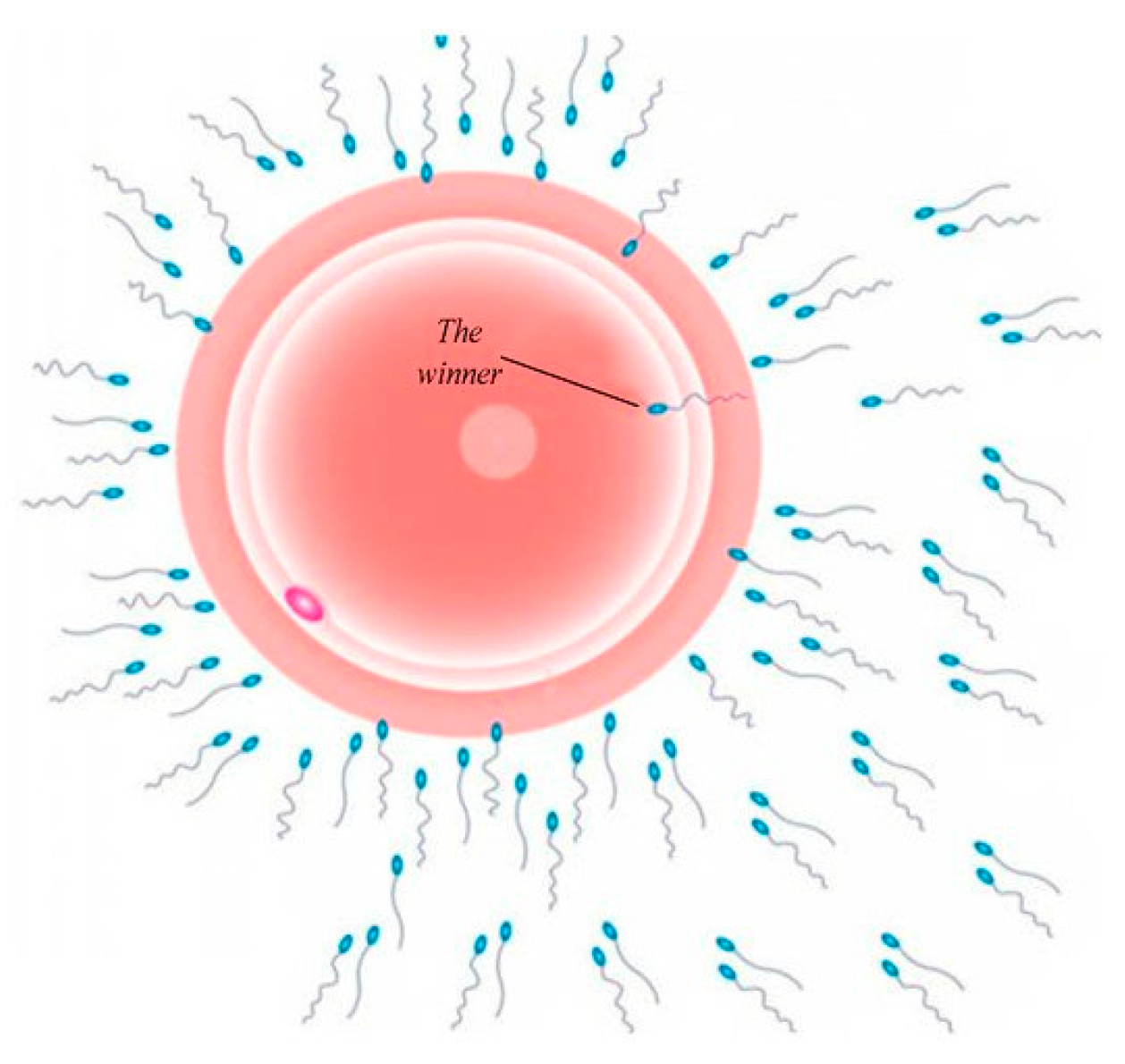
Usually, in a typical scenario, one sperm can fertilize an ovum. Based on that, Shehadeh et al. [2,5,6,7,8] calls this sperm the winner. The winner and the flock of sperm are illustrated in Figure 2.
The best answer is found and obtained using this strategy, which makes use of a group of sperm (potential solutions) floating over the whole search area. Concurrently, the possible solutions will consider the most suitable sperm in their path, who will be the victor (the sperm that is closest to the egg). Alternatively, the flock will consider on the winner’s position and the position of its prior best solution. Thus, every sperm enhances its initial zone across the optimum area by taking into consideration its current velocity, current location, and the location of both the global’s best solution (the winner) and the sperm’s best solution. Mathematically speaking, in SSO, the flock updated their sites according to the following formula:
where
- vi is the velocity of potential solution i at iteration t;
- xi is the current position of possible solution i at iteration t;
Three velocities can be used to calculate the sperm’s velocity: the initial velocity of a potential solution, the personal best solution, and the global best solution.
First is the initial velocity of sperm, which takes a random value based on the velocity dumping parameter and the pH value of the initial location. The model can be calculated by applying the following formula:
Second is a personal best location for the potential solution, adjusted in memory based on the prior location until it is closest to the optimal value. However, this velocity can be changed based on the pH and temperature values. The following formula may be used to calculate this model:
Third, the global best solution is simulated by the winner, which is denoted by the closest sperm to the ovum. The mathematical model of the winning velocity of the potential solution Vi(t) can be represented in Equation (4). The flock of sperm and the value of the winner are depicted in Figure 2.
The symbols of the prior equations are as follows:
- vi is the velocity of potential solution i at iteration t;
- D is the velocity damping factor and is a random parameter with a range of 0 to 1;
- pH_Rand1, pH_Rand2, and pH_Rand3 are the reached site pH values, which are random parameters that take values between 7 to 14;
- Temp_Rand1 and Temp_Rand2 are values of the site temperature, which are random parameters that take values between 35.1 to 38.5;
- xi is the current position of potential solution i at iteration t;
- xsbest is the personal best location of potential solution i at iteration t;
- xsgbest is the global best location of the flock.
Based on the equations mentioned above, the total velocity rule Vi(t) can be formalized based on velocity initial value, personal best solution, and global best solution as follows [2,5,6,7,8]:
Based on the theory of SSO, both pH and temperature affect the velocity rule. The pH changes depending on the woman’s attitude, whether depressed or happy, and on the food consumed. The value of the pH parameter falls in a range between seven and fourteen. Alternatively, the temperature ranges from 35.1 to 38.5 °C according to blood pressure circulation in the reproductive system [7].
Further, SSO is a swarm-based method that simulates the metaphor of natural fertilization. SSO, however, has a few disadvantages in terms of efficiency. Applied to a broad search domain, SSO is prone to getting trapped in local optima [2], which is one of its main drawbacks. Therefore, improvements are needed to enhance the method’s exploration process.
2.2. Newton’s Method
An iterative technique is a technique (method) for finding an approximate solution by making successive approximations. Iterative approaches usually cannot deliver accurate answers. Accordingly, researchers generally select a tolerance level to distinguish between approximate and exact answers for the solutions obtained through iterative approaches. Newton’s method, also known as the Newton–Raphson method, was proposed by Isaac Newton and is the most widely used iterative method. The procedure of Newton’s scheme is described by
where is the nonlinear system of equations, and represents the “Jacobian of ″. Newton’s second-order convergence method may be easily applied to various nonlinear algebraic problems [1]. As a result, mathematical tools such as Mathematica and MATLAB provide built-in routines for finding nonlinear equations’ roots based on Newton’s scheme.
3. Modified Sperm Swarm Optimization (MSSO)
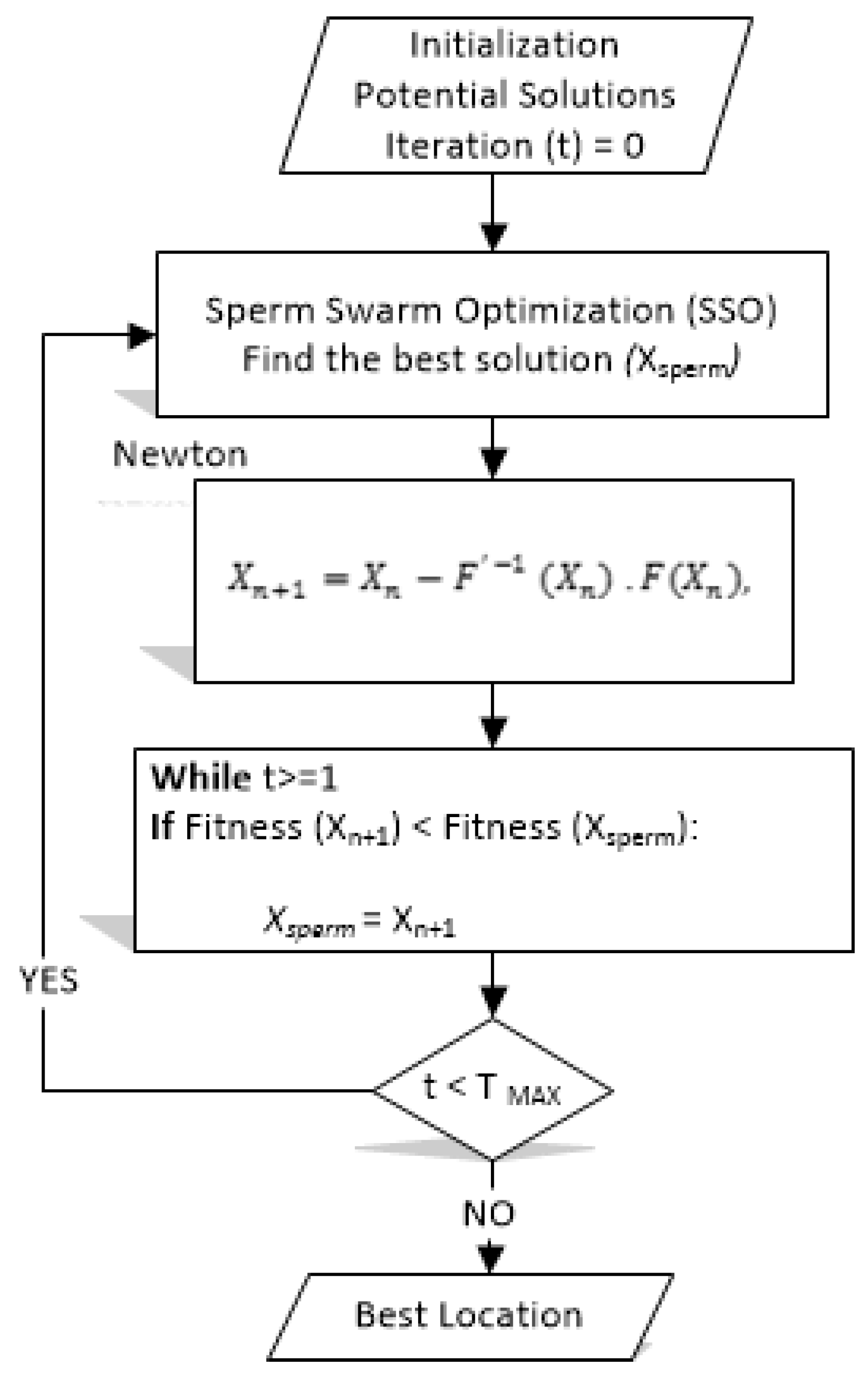
SSO is a powerful optimization technique that can address various issues. No algorithm, however, is suitable for tackling all problems, according to the “No Free Lunch (NFL)” theorem [48]. By using Newton’s method, the proposed MSSO outperforms the original SSO in terms of solving nonlinear equation systems. In MSSO, Newton’s methods are used as a local search to enhance the search process, as shown in Figure 3.
When Newton’s method is applied to the sperm position, at each iteration, the fitness value of the potential solution is compared to the fitness of the location calculated by Newton’s scheme. The newly computed location by Newton’s method is shown in Figure 3 as .
In each iteration, MSSO employs both the SSO algorithm and Newton’s method. The SSO first determines the most optimal sperm location among the twenty initial locations as an optimal candidate location. The optimal candidate location is then fed into Newton’s method. In other words, the output from SSO is considered a potential solution or a temporary solution. The obtained solution is then treated as an input for Newton’s method. Newton’s method as an iterative method calculates the next candidate solution based on Equation (6). Newton’s method’s ability to find a better candidate is very high since it is a second-order convergence method. However, in order to avoid a local optimal solution, the candidate solution obtained from Newton’s method (Xn+1) is compared to the solution calculated by SSO (Xsperm). Thus, the location with the lowest fitness value determines the potential solution to the problem. The next iteration is then performed based on the current most promising solution. Algorithm 1 shows the pseudocode for the suggested MSSO algorithm.
| Algorithm 1. Modified Sperm Swarm Optimization (MSSO). | |
| Begin | |
| Step 1: | Initialize potential solutions. |
| Step 2: | for i = 1: size of flock do |
| Step 3: | apply the fitness for potential solution. |
| if obtained fitness > best solution of the potential solution then | |
| give the current value as the best solution of the potential solution. | |
| end if | |
| end for | |
| Step 4: | depends on the winner, give the value of winner. |
| Step 5: | for i =1: size of flock do |
| Perform Equation (5) | |
| Perform Equation (1). | |
| end for | |
| Step 6: | Calculate Newton’s location using Equation (6) |
| Calculate the fitness of and using Equation (7) | |
| if fitness () < fitness | |
| end if | |
| Step 7: | while final iterations is not reached go to Step 2. |
| End. | |
The initialization, exploitation, and exploration phases of the SSO method are shown in the algorithm. The alterations specified in the red box are implemented at the end of each iteration. We compare Newton’s location with the sperm’s optimal location based on their fitness values and select the one that has the best fitness value.
Computational Complexity
The complexity of the new MSSO’s can be obtained by adding up the SSO’s complexity and Newton’s method’s complexity. At first glance, Newton’s technique is overly complicated compared to optimization methods. At each iteration, one has to solve a system of linear models, which is time-consuming because every Jacobian calculation requires scalar function evaluations. As a result, combining Newton’s approach with any optimization process is likely to make it more complicated.
On the other hand, combining SSO with Newton’s technique did not significantly increase processing time. However, the MSSO can overcome Newton’s method limitations, including selecting the starting points and divergence difficulties. As a result, the MSSO is superior at solving nonlinear equation systems.
The MSSO’s time complexity is influenced by the initial phase, the process of updating the position of the sperm, and the use of Newton’s scheme. The complexity of the initialization process is O(S), where S is the total number of sperm. The updating process, which includes determining the optimal solution and updating sperm positions, has a complexity equal to O(I × S) + O(I × S × M), where I and M represent the maximum number of iterations and the complexity of the tested benchmark equation respectively. Furthermore, Newton’s scheme complexity is calculated as O(I × T), where T is the computation time. Consequently, the proposed MSSO has an overall computational complexity of O(S × (I + IM + 1) + IT).
Every improvement certainly has a cost. The principal objective of the proposed hybrid algorithm is to enhance the fitness value and the convergence speed of the existing algorithms. However, as a result of adding one algorithm to another, the complexity and the time cost of the hybrid algorithm are increased compared to the original algorithm. Eventually, a tradeoff between the merits and disadvantages should be considered while using any algorithm.
4. Numerical Tests
Eight nonlinear systems of several orders were selected as indicators to clarify the efficiency and capability of the new hybrid MSSO scheme. Comparisons between MSSO and the other six well-known optimization algorithms have been performed. Those optimization algorithms are the original SSO [2], HHO [9], PSO [49], ALO [10], BOA [11], and EO [13]. For consistency, all selected systems used in the comparisons are arbitrary problems that are common in the literature, for instance, [19,21,40,44,50,51,52,53].
The comparison between the optimization algorithms is based on the fitness value of each algorithm in each benchmark. A solution with less fitness value is more accurate than a solution with a higher fitness value. Hence, the most effective optimization algorithm is the one that solves with the least fitness value. The fitness function used in the comparison is the Euclidean norm, also called the square norm or norm-2. Using the Euclidean norm, we can determine the distance from the origin, which is expressed as follows:
Similar settings have been used in all benchmarks to guarantee a fair comparison of all selected algorithms. The parameter values of all optimization algorithms have been fine-tuned to improve the performance of the algorithms. The best solution was chosen by every optimization method 30 times. Search agents (population size) have been set to 20 and the maximum iteration to 50. Furthermore, the best solution with the least fitness value is chosen if there is more than one solution for a particular benchmark. In the end, for lack of space, answers are shortened to 11 decimal places.
Calculations were conducted using MATLAB software version R2020a with the default variable precision of 16 digits. This was on an Intel Core i5 processor running at 2.2 GHz and 8 GB of RAM under the Microsoft Windows 8 operating system.
Problem 1: Let us consider the first problem to be the following nonlinear system of two equations:
For this system, the precise solution is given by , . After running the algorithms 30 times, MSSO significantly surpassed all other optimization algorithms in the comparison. Table 1 shows that the proposed hybrid MSSO algorithm has attained the best solution with the least fitness value equaling zero. This means that the solution obtained by MSSO is an exact solution for the given system.
Problem 2: The second benchmark is the system of two nonlinear equations given by:
Here, the exact zero for the system in this problem is given by . As shown in Table 2, it is evident that MSSO achieved the exact solution of this system with a fitness value of zero. It also outperformed all other algorithms with a substantial difference, especially in comparison with SSO, BOA, and HHO.
Problem 3: The third system of nonlinear equations is given by:
This NES of three equations has the exact solution , , . According to Table 3, the proposed MSSO achieved a zero fitness value. The superiority of MSSO is evident in this example, with a significant difference between MSSO and all other compared optimization algorithms.
Problem 4: Consider the following system of three nonlinear equations:
The precise solution of the nonlinear system in this problem is equal to . The best solution achieved by the compared schemes for the given system is illustrated in Table 4. The proposed MSSO found a precise answer, with zero as a fitness value. ALO recorded the second-best solution with a fitness value of 2.27 × 10⁻⁶, while the rest of the compared algorithms were far from the exact answer. Again, the proposed MSSO has proved it has an efficient local search mechanism. Hence, it can achieve more accurate solutions for nonlinear systems.
Problem 5: The next benchmark is the following system of two nonlinear equations:
This nonlinear system has the trivial solution . Table 5 illustrates the comparison between the different optimization algorithms for the given system. Compared with the other algorithms, the original SSO and HHO achieved excellent results, with fitness values of 5.36 × 10⁻¹⁵ and 6.92 × 10⁻¹⁴, respectively. However, MSSO outperformed both of them and delivered the exact solution for the given system.
Problem 6: The sixth system considered for the comparison is an interval arithmetic benchmark [53] given by the following system of ten equations:
In this benchmark, MSSO has proven its efficiency. Table 6 clearly shows the significant differences between MSSO and the other compared algorithms. MSSO achieved the best solution with a fitness value of 5.21 × 10⁻¹⁷, while all different algorithms achieved solutions far from the exact answer. When we compare the fitness values of the hybrid MSSO and the original SSO, we can see how substantial modifications were made to the local search mechanism of the original SSO to produce the hybrid MSSO.
Problem 7: Consider the model A combustion chemistry problem for a temperature of 3000 °C [21], which can be described by the following nonlinear system of equations:
In Table 7, the comparison for this system shows that MSSO has the least fitness value of 7.09 × 10⁻²¹, while PSO and EO have fitness values of 2.85 × 10⁻⁹ and 3.45 × 10⁻⁸, respectively.
Problem 8: The last benchmark is an application from neurophysiology [52], described by the nonlinear system of six equations:
There is more than one exact solution to this system. Table 8 shows that the proposed MSSO algorithm achieved the most accurate solution with a fitness value of 1.18 × 10⁻²⁴, and the PSO algorithm achieved second place with a fitness value of 5.26 × 10⁻⁷. In contrast, the rest of the algorithms recorded answers that differ significantly from the exact solution. Further, NESs in problems 6–8 prove the flexibility of the proposed hybrid MSSO as it remains efficient even in a wide interval [−10, 10].
The comparison results in all benchmarks confirm the hypothesis that we have mentioned in the first section; that is, that the hybridization of two algorithms inherits the efficient merits of both algorithms (SSO and Newton’s methods). This can be seen by looking at the comparison results between the MSSO and the original SSO, where the MSSO has outperformed the original SSO in all selected benchmarks. The reason for this remarkable performance is the use of Newton’s method as a local search, which strengthens the hybrid’s capability to avoid the local optimum in Problems 1–5 (where MSSO has obtained the exact solution), and significantly improves the obtained fitness values in Problems 6-8. The comparisons indicate that the proposed hybrid algorithm MSSO has avoided being trapped in the local optima in all problems, compared with the majority of the other algorithms.
5. Results and Analysis
5.1. Stability and Consistency of MSSO
Table 9 shows the average fitness value of the MSSO and the other algorithms compared in the previous benchmarks. This is when each problem is run 30 times to illustrate the continuous efficiency and power of the proposed MSSO algorithm.
According to Table 9, MSSO has surpassed all other compared algorithms. The average fitness values of MSSO and the original SSO show a significant difference in all benchmarks. Consequently, this improvement confirms the flexibility of the hybrid MSSO in seeking the best solution without being entrapped by local optima. Furthermore, as shown in Table 9, MSSO outperforms all of the other compared algorithms, particularly for problems 2, 4, 6, and 8.
Additionally, the algorithm is considered consistent and stable if it maintains consistency over 30 runs. The average of the solutions must, therefore, be the same as or very close to the best solution in order to achieve consistency. It has been demonstrated in this study that MSSO consistency has been maintained for all selected problems. Moreover, the average standard deviation achieved by each algorithm is shown in Table 10, in which smaller values of standard deviation indicate more stability. The hybrid MSSO demonstrated stable results in most of the selected problems.
Furthermore, the significance of MSSO improvements was examined using the statistical t-test in Table 11. Improvements were considered significant if the p-value was less than 0.05; otherwise, they were not. Results show that all algorithms have p-values lower than 0.05 in all tested problems, except for HHO, which has a single value above 0.05 in Problem 5. It is evident from this that MSSO has a higher level of reliability than competing algorithms. Further, MSSO’s solutions are significantly more accurate than those of other algorithms since the majority of its p-values are close to 0. The results demonstrate that the MSSO is a robust search method capable of finding precise solutions. Moreover, it is able to avoid local optimal traps and immature convergence.
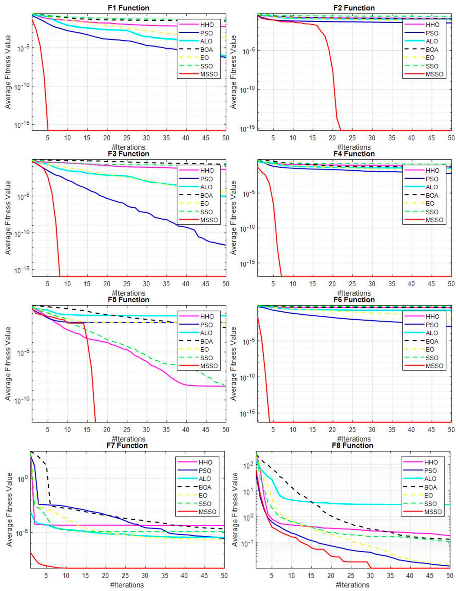
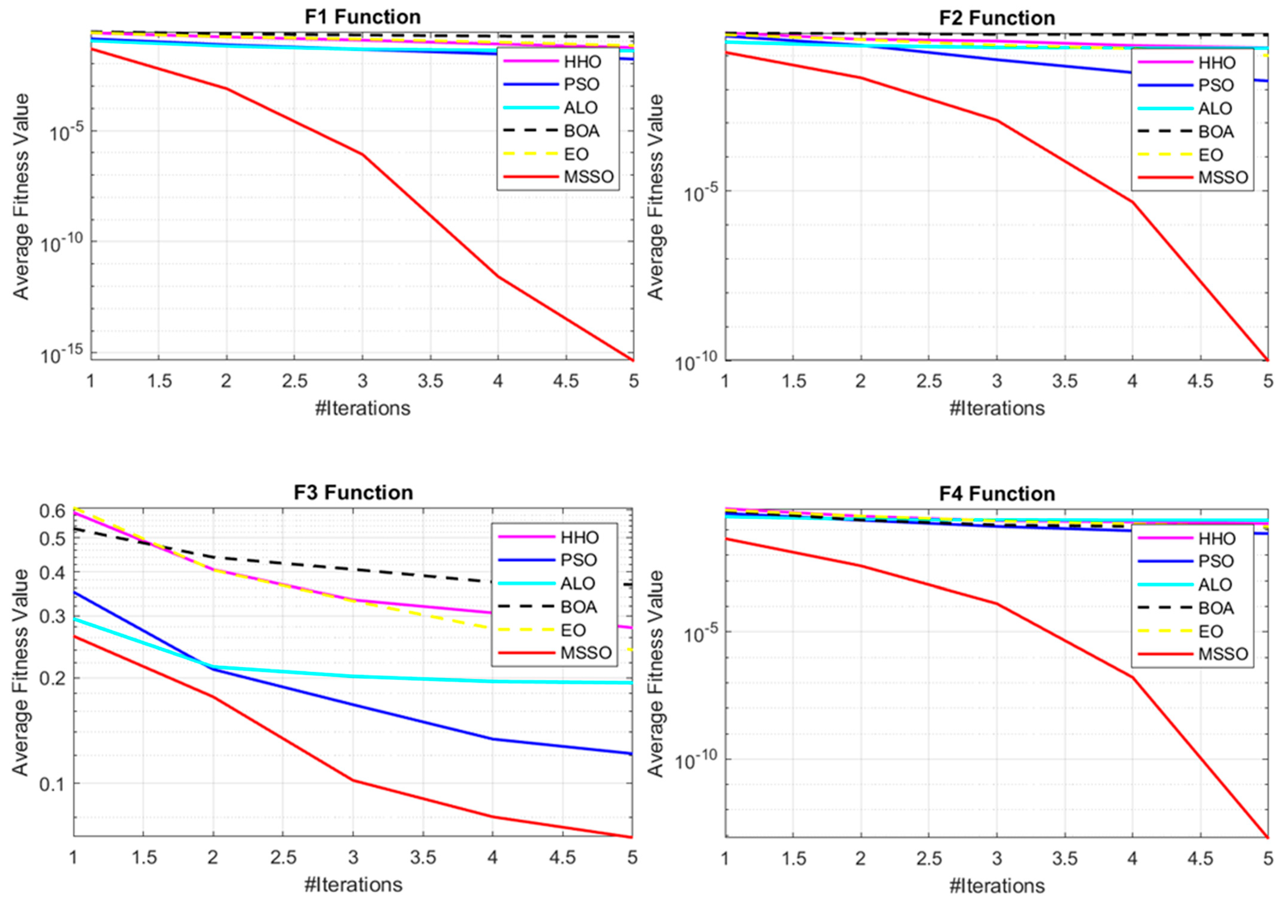
Moreover, one of the criteria that is considered when comparing algorithms is their speed of convergence. Figure 4 indicates that MSSO enhanced the convergence speed of the original SSO in all problems. It also shows that MSSO achieves the best solution with much fewer iterations than the other algorithms. Consequently, the superiority of the proposed MSSO is confirmed.
It is known that any optimization method has some constraints that slow down the algorithm from finding the optimum solution or, in some cases, prevent it from finding the solution. HHO, for instance, probably attains local optima instead of the optimal answer. SSO quickly falls into a local minimum of systems of nonlinear equations, which consists of a set of models [2]. PSO has some drawbacks, such as a lack of population variety and the inability to balance local optima and global optima [54]. The EO method, on the other hand, does not function well for large-scale situations [55].
The novel hybrid algorithm MSSO’s convergence speed is attributed to combining Newton’s iterative method as a local search and the SSO algorithm. On the one hand, MSSO benefits from the originality of Newton’s method, which was developed to find solutions to nonlinear equation systems. On the other hand, SSO ensures appropriate initial solutions for Newton’s method by employing search agents. Furthermore, Newton’s method features a second-order of convergence, which implies that the scheme converges to approximately two significant digits in each iteration [1]. Thus, the hybridization between Newton’s method and the SSO algorithm inherits the merits from both sides to produce an efficient algorithm that can overcome the main disadvantages [56,57].
It is worth noting that the default precision value of the variable in MATLAB was used for all calculations in this study, which is 16 digits of precision. This precision is timesaving compared with more significant digits. However, in some situations, this may impact the outcome. In MATLAB, the function ”vpa” may be used to enhance variable precision. Thus, increasing the number of digits can improve the accuracy of the findings, but this is a time-consuming operation. More details and examples of this case can be seen in [40]. In this research, the use of ”vpa” has increased the accuracy of the results in Problem 5, Problem 7, and Problem 8.
5.2. Comparison between MSSO and Newton’s Method
The effectiveness of MSSO is demonstrated by the correctness of the generated solutions and its ability to avoid local optima compared to Newton’s method. Accordingly, both strategies were examined for problems 1–4. Table 12, Table 13, Table 14 and Table 15 compare the fitness values achieved by MSSO and Newton’s method using three randomly chosen starting points. We examined both strategies for comparison purposes at iteration 5, iteration 7, and iteration 10. In addition, variables of 1200-digit precision in all selected problems were used to clarify the solutions’ accuracy. If, as noted earlier, the number of digits is increased, the findings may also improve.
MSSO surpassed Newton’s approach in all of the chosen problems, as shown in Table 12, Table 13, Table 14 and Table 15. Newton’s method, like all other iterative methods, is extremely sensitive to the starting answer . Choosing an incorrect starting point can slow down the convergence of Newton’s method (see Table 12 and Table 14) or cause Newton’s method to diverge (see Table 13). Further, a singularity in the Jacobian in Newton’s method’s denominator can be caused by the improper selection of the initial point. The Jacobian’s inverse does not thus exist. Therefore, it is impossible to utilize Newton’s approach (refer to Table 14 and Table 15).
Table 12, Table 13, Table 14 and Table 15 show a considerable improvement in MSSO outcomes compared with Newton’s technique. The primary issue with Newton’s starting point has been addressed by relying on 20 search agents at the early stages of the hybrid MSSO. This is rather than picking one point as Newton does. The MSSO selects several random starting points, called search agents, unlike Newton’s method. MSSO examines each search agent’s fitness value, then chooses the search agent with the lowest fitness value as an initial guess. Selecting the starting point in this manner is crucial for improving the accuracy of the answer.
The previous experiments show that the proposed MSSO outperforms Newton’s method in selected problems. As opposed to Newton’s method, which normally starts with one initial point, MSSO starts with 20 search agents. The superiority of the MSSO is demonstrated by the accuracy of its solutions. In addition, the time required to reach the convergence criteria is less in MSSO. Having 20 random initial solutions clearly requires more time for Newton’s method. Therefore, this is another reason why hybridizing both SSO and Newton’s method is better than depending on one of them.
Moreover, the speed of convergence towards the best solution is astonishing. MSSO can choose the best initial point in a few iterations and move quickly toward the global optima. Figure 5 shows the convergence speed of problems 1–4 for the first five iterations on an average of 30 runs.
To clarify the significant improvements of MSSO over Newton’s iterative method, a comparison between Newton’s technique and MSSO for Problems 1, 2, 3, and 4 were performed. Table 16 shows the CPU-time needed for Newton’s technique and MSSO to attain the stopping criterion (ε ≤ 1 × 10⁻¹⁵).
Based on the results, an apparent enhancement has been added to Newton’s method by using the hybridized MSSO. The CPU-time needed to satisfy the selected stopping limit is much better for MSSO than Newton’s method. Even though Newton’s method is a part of the proposed MSSO, MSSO showed better results because of the mechanism of SSO in selecting the best initial guess for Newton’s technique as a local search inside the hybrid algorithm.
It is well known that choosing a starting point that is far from the root of the system could negatively affect the convergence of Newton’s method. Therefore, since Newton’s method is included in the MSSO, this could negatively affect MSSO’s convergence as well. However, based on the mechanism of the MSSO, the algorithm randomly selects 20 agents that are considered as initial points within a specific interval. In general, optimization algorithms have more choices to start with compared to Newton’s method. Iterative methods can benefit from hybridization in selecting initial points because optimization algorithms can have many initial points. On the other hand, optimization algorithms can benefit from the fast and accurate convergence of iterative methods.
6. Conclusions
In this work, a hybrid method known as MSSO was introduced for solving systems of nonlinear equations using Newton’s iterative method as a local search for the Sperm Swarm Optimization algorithm SSO. The main goal of the MSSO is to solve the problem of Newton’s method’s initial guess, the achievement of which results in a better selection of initial points, enabling it to be applied to a wider variety of real-world applications. Moreover, Newton’s scheme was used in MSSO as a local search, which improved the accuracy of the tested solutions. In addition, the MSSO’s convergence speed is substantially improved.
Eight nonlinear systems of varying orders were utilized to illustrate the effectiveness of the proposed MSSO. The novel MSSO was also compared to six well-known optimization methods, including the original SSO, BOA, ALO, EO, HHO, and PSO. The Euclidean norm has been utilized as a fitness function in all benchmarks. According to the results, MSSO outperforms all other compared algorithms in four metrics: fitness value, solution accuracy, stability, and speed of convergence. In addition, the consistency of the MSSO is confirmed by running the methods thirty times. Additionally, the standard deviation showed that MSSO was the most stable optimization algorithm.
Additionally, we compared the performance of MSSO and Newton’s method on four problems from the benchmarks. Across all four datasets, the MSSO outperformed Newton’s method. The MSSO method also overcomes some of Newton’s scheme’s limitations, such as divergence and selection of initial guesses.
Future work can address some related issues, such as how the suggested method performs against common optimization benchmarks. Future research will also focus on solving nonlinear equations arising from real-world applications, such as Burgers’ Equation. In addition, future work needs to address the efficiency of the proposed algorithm when solving big systems. Finally, the use of a derivative-free iterative method instead of Newton’s method reduces the computational complexity resulting from the need to evaluate Newton’s method in each iteration and is an interesting topic that needs to be focused on in the future.
Author Contributions
Conceptualization, O.S.S. and R.S.; methodology, O.S.S., R.S. and H.S.; validation, K.A. and I.H.; formal analysis, O.S.S. and R.S.; investigation, O.S.S. and R.S.; resources, O.S.S., R.S. and H.S.; data curation, O.S.S. and R.S.; writing—original draft preparation, O.S.S., R.S. and H.S.; writing—review and editing, K.A. and I.H.; visualization, R.S.; supervision, O.S.S., R.S. and I.H.; project administration, O.S.S., R.S. and I.H.; funding acquisition, I.H. All authors have read and agreed to the published version of the manuscript.
Funding
This research and the APC were funded by Universiti Kebangsaan Malaysia, grant number DIP-2021-018.
Data Availability Statement
The data that support the findings of this study are available on request from the corresponding author, Sihwail, R.
Conflicts of Interest
The authors declare that there is no conflict of interest regarding the publication of this paper.
References
- Traub, J.F. Iterative Methods for the Solution of Equations; Prentice-Hall: Englewood Cliffs, NJ, USA, 1964. [Google Scholar]
- Shehadeh, H.A. A Hybrid Sperm Swarm Optimization and Gravitational Search Algorithm (HSSOGSA) for Global Optimization. Neural Comput. Appl. 2021, 33, 11739–11752. [Google Scholar] [CrossRef]
- Gupta, S. Enhanced Harmony Search Algorithm with Non-Linear Control Parameters for Global Optimization and Engineering Design Problems. Eng. Comput. 2022, 38, 3539–3562. [Google Scholar] [CrossRef]
- Zhu, F.; Chen, D.; Zou, F. A Novel Hybrid Dynamic Fireworks Algorithm with Particle Swarm Optimization. Soft Comput. 2021, 25, 2371–2398. [Google Scholar] [CrossRef]
- Shehadeh, H.A.; Ahmedy, I.; Idris, M.Y.I. Empirical Study of Sperm Swarm Optimization Algorithm. Adv. Intell. Syst. Comput. 2018, 869, 1082–1104. [Google Scholar] [CrossRef]
- Shehadeh, H.A.; Ahmedy, I.; Idris, M.Y.I. Sperm Swarm Optimization Algorithm for Optimizing Wireless Sensor Network Challenges. In Proceedings of the 6th International Conference on Communications and Broadband Networking, Singapore, 24–26 February 2018; pp. 53–59. [Google Scholar] [CrossRef]
- Shehadeh, H.A.; Idris, M.Y.I.; Ahmedy, I.; Ramli, R.; Noor, N.M. The Multi-Objective Optimization Algorithm Based on Sperm Fertilization Procedure (MOSFP) Method for Solving Wireless Sensor Networks Optimization Problems in Smart Grid Applications. Energies 2018, 11, 97. [Google Scholar] [CrossRef] [Green Version]
- Id, H.A.S.; Yamani, M.; Idris, I.; Ahmedy, I. Multi-Objective Optimization Algorithm Based on Sperm Fertilization Procedure (MOSFP). Symmetry 2017, 9, 241. [Google Scholar] [CrossRef] [Green Version]
- Heidari, A.A.; Mirjalili, S.; Faris, H.; Aljarah, I.; Mafarja, M.; Chen, H. Harris Hawks Optimization: Algorithm and Applications. Future Gener. Comput. Syst. 2019, 97, 849–872. [Google Scholar] [CrossRef]
- Mirjalili, S. The Ant Lion Optimizer. Adv. Eng. Softw. 2015, 83, 80–98. [Google Scholar] [CrossRef]
- Arora, S.; Singh, S. Butterfly Optimization Algorithm: A Novel Approach for Global Optimization. Soft Comput. 2018, 23, 715–734. [Google Scholar] [CrossRef]
- Zhang, Y.; Wang, Y.H.; Gong, D.W.; Sun, X.Y. Clustering-Guided Particle Swarm Feature Selection Algorithm for High-Dimensional Imbalanced Data With Missing Values. IEEE Trans. Evol. Comput. 2022, 26, 616–630. [Google Scholar] [CrossRef]
- Faramarzi, A.; Heidarinejad, M.; Stephens, B.; Mirjalili, S. Equilibrium Optimizer: A Novel Optimization Algorithm. Knowl.-Based Syst. 2020, 191, 105190. [Google Scholar] [CrossRef]
- Holland, J.H. Genetic Algorithms. Sci. Am. 1992, 267, 66–72. [Google Scholar] [CrossRef]
- Liu, K.; Hu, X.; Yang, Z.; Xie, Y.; Feng, S. Lithium-Ion Battery Charging Management Considering Economic Costs of Electrical Energy Loss and Battery Degradation. Energy Convers. Manag. 2019, 195, 167–179. [Google Scholar] [CrossRef]
- Liu, K.; Zou, C.; Li, K.; Wik, T. Charging Pattern Optimization for Lithium-Ion Batteries with an Electrothermal-Aging Model. IEEE Trans. Ind. Inform. 2018, 14, 5463–5474. [Google Scholar] [CrossRef]
- Zhou, R.H.; Li, Y.G. An Improve Cuckoo Search Algorithm for Solving Nonlinear Equation Group. Appl. Mech. Mater. 2014, 651–653, 2121–2124. [Google Scholar] [CrossRef]
- Ariyaratne, M.K.A.; Fernando, T.G.I.; Weerakoon, S. Solving Systems of Nonlinear Equations Using a Modified Firefly Algorithm (MODFA). Swarm Evol. Comput. 2019, 48, 72–92. [Google Scholar] [CrossRef]
- Ren, H.; Wu, L.; Bi, W.; Argyros, I.K. Solving Nonlinear Equations System via an Efficient Genetic Algorithm with Symmetric and Harmonious Individuals. Appl. Math. Comput. 2013, 219, 10967–10973. [Google Scholar] [CrossRef]
- Chang, W. der An Improved Real-Coded Genetic Algorithm for Parameters Estimation of Nonlinear Systems. Mech. Syst. Signal Process. 2006, 20, 236–246. [Google Scholar] [CrossRef]
- Grosan, C.; Abraham, A. A New Approach for Solving Nonlinear Equations Systems. IEEE Trans. Syst. Man Cybern. Part ASyst. Hum. 2008, 38, 698–714. [Google Scholar] [CrossRef]
- Jaberipour, M.; Khorram, E.; Karimi, B. Particle Swarm Algorithm for Solving Systems of Nonlinear Equations. Comput. Math. Appl. 2011, 62, 566–576. [Google Scholar] [CrossRef] [Green Version]
- Mo, Y.; Liu, H.; Wang, Q. Conjugate Direction Particle Swarm Optimization Solving Systems of Nonlinear Equations. Comput. Math. Appl. 2009, 57, 1877–1882. [Google Scholar] [CrossRef] [Green Version]
- Sihwail, R.; Omar, K.; Ariffin, K.A.Z. An Effective Memory Analysis for Malware Detection and Classification. Comput. Mater. Contin. 2021, 67, 2301–2320. [Google Scholar] [CrossRef]
- Sihwail, R.; Omar, K.; Zainol Ariffin, K.; al Afghani, S. Malware Detection Approach Based on Artifacts in Memory Image and Dynamic Analysis. Appl. Sci. 2019, 9, 3680. [Google Scholar] [CrossRef] [Green Version]
- Jadon, S.S.; Tiwari, R.; Sharma, H.; Bansal, J.C. Hybrid Artificial Bee Colony Algorithm with Differential Evolution. Appl. Soft Comput. J. 2017, 58, 11–24. [Google Scholar] [CrossRef]
- Jia, R.; He, D. Hybrid Artificial Bee Colony Algorithm for Solving Nonlinear System of Equations. In Proceedings of the 2012 8th International Conference on Computational Intelligence and Security, CIS 2012, Guangzhou, China, 17–18 November 2012; pp. 56–60. [Google Scholar]
- Aydilek, İ.B. A Hybrid Firefly and Particle Swarm Optimization Algorithm for Computationally Expensive Numerical Problems. Appl. Soft Comput. J. 2018, 66, 232–249. [Google Scholar] [CrossRef]
- Nasr, S.; El-Shorbagy, M.; El-Desoky, I.; Hendawy, Z.; Mousa, A. Hybrid Genetic Algorithm for Constrained Nonlinear Optimization Problems. Br. J. Math. Comput. Sci. 2015, 7, 466–480. [Google Scholar] [CrossRef]
- Abualigah, L.M.; Khader, A.T.; Hanandeh, E.S.; Gandomi, A.H. A Novel Hybridization Strategy for Krill Herd Algorithm Applied to Clustering Techniques. Appl. Soft Comput. J. 2017, 60, 423–435. [Google Scholar] [CrossRef]
- El-Shorbagy, M.A.; Mousa, A.A.A.; Fathi, W. Hybrid Particle Swarm Algorithm for Multiobjective Optimization: Integrating Particle Swarm Optimization with Genetic Algorithms for Multiobjective Optimization; Lambert Academic: Saarbrücken, Germany, 2011. [Google Scholar]
- Goel, R.; Maini, R. A Hybrid of Ant Colony and Firefly Algorithms (HAFA) for Solving Vehicle Routing Problems. J. Comput. Sci. 2018, 25, 28–37. [Google Scholar] [CrossRef]
- Turanoğlu, B.; Akkaya, G. A New Hybrid Heuristic Algorithm Based on Bacterial Foraging Optimization for the Dynamic Facility Layout Problem. Expert Syst. Appl. 2018, 98, 93–104. [Google Scholar] [CrossRef]
- Skoullis, V.I.; Tassopoulos, I.X.; Beligiannis, G.N. Solving the High School Timetabling Problem Using a Hybrid Cat Swarm Optimization Based Algorithm. Appl. Soft Comput. J. 2017, 52, 277–289. [Google Scholar] [CrossRef]
- Chen, X.; Zhou, Y.; Tang, Z.; Luo, Q. A Hybrid Algorithm Combining Glowworm Swarm Optimization and Complete 2-Opt Algorithm for Spherical Travelling Salesman Problems. Appl. Soft Comput. J. 2017, 58, 104–114. [Google Scholar] [CrossRef]
- Marichelvam, M.K.; Tosun, Ö.; Geetha, M. Hybrid Monkey Search Algorithm for Flow Shop Scheduling Problem under Makespan and Total Flow Time. Appl. Soft Comput. J. 2017, 55, 82–92. [Google Scholar] [CrossRef]
- Karr, C.L.; Weck, B.; Freeman, L.M. Solutions to Systems of Nonlinear Equations via a Genetic Algorithm. Eng. Appl. Artif. Intell. 1998, 11, 369–375. [Google Scholar] [CrossRef]
- Luo, Y.Z.; Yuan, D.C.; Tang, G.J. Hybrid Genetic Algorithm for Solving Systems of Nonlinear Equations. Chin. J. Comput. Mech. 2005, 22, 109–114. [Google Scholar]
- Luo, Y.Z.; Tang, G.J.; Zhou, L.N. Hybrid Approach for Solving Systems of Nonlinear Equations Using Chaos Optimization and Quasi-Newton Method. Appl. Soft Comput. J. 2008, 8, 1068–1073. [Google Scholar] [CrossRef]
- Sihwail, R.; Said Solaiman, O.; Omar, K.; Ariffin, K.A.Z.; Alswaitti, M.; Hashim, I. A Hybrid Approach for Solving Systems of Nonlinear Equations Using Harris Hawks Optimization and Newton’s Method. IEEE Access 2021, 9, 95791–95807. [Google Scholar] [CrossRef]
- Sihwail, R.; Said Solaiman, O.; Zainol Ariffin, K.A. New Robust Hybrid Jarratt-Butterfly Optimization Algorithm for Nonlinear Models. J. King Saud Univ.—Comput. Inf. Sci. 2022, 34 Pt A, 8207–8220. [Google Scholar] [CrossRef]
- Sihwail, R.; Omar, K.; Ariffin, K.A.Z.; Tubishat, M. Improved Harris Hawks Optimization Using Elite Opposition-Based Learning and Novel Search Mechanism for Feature Selection. IEEE Access 2020, 8, 121127–121145. [Google Scholar] [CrossRef]
- Said Solaiman, O.; Hashim, I. Efficacy of Optimal Methods for Nonlinear Equations with Chemical Engineering Applications. Math. Probl. Eng. 2019, 2019, 1728965. [Google Scholar] [CrossRef] [Green Version]
- Said Solaiman, O.; Hashim, I. An Iterative Scheme of Arbitrary Odd Order and Its Basins of Attraction for Nonlinear Systems. Comput. Mater. Contin. 2020, 66, 1427–1444. [Google Scholar] [CrossRef]
- Said Solaiman, O.; Hashim, I. Optimal Eighth-Order Solver for Nonlinear Equations with Applications in Chemical Engineering. Intell. Autom. Soft Comput. 2021, 27, 379–390. [Google Scholar] [CrossRef]
- Said Solaiman, O.; Hashim, I. Two New Efficient Sixth Order Iterative Methods for Solving Nonlinear Equations. J. King Saud Univ. Sci. 2019, 31, 701–705. [Google Scholar] [CrossRef]
- Said Solaiman, O.; Ariffin Abdul Karim, S.; Hashim, I. Dynamical Comparison of Several Third-Order Iterative Methods for Nonlinear Equations. Comput. Mater. Contin. 2021, 67, 1951–1962. [Google Scholar] [CrossRef]
- Adam, S.P.; Alexandropoulos, S.A.N.; Pardalos, P.M.; Vrahatis, M.N. No Free Lunch Theorem: A Review. Springer Optim. Its Appl. 2019, 145, 57–82. [Google Scholar] [CrossRef]
- Kennedy, J.; Eberhart, R. Particle Swarm Optimization. In Proceedings of the ICNN’95—International Conference on Neural Networks, Perth, WA, Australia, 27–1 December 1995; pp. 1942–1948. [Google Scholar] [CrossRef]
- El-Shorbagy, M.A.; El-Refaey, A.M. Hybridization of Grasshopper Optimization Algorithm with Genetic Algorithm for Solving System of Non-Linear Equations. IEEE Access 2020, 8, 220944–220961. [Google Scholar] [CrossRef]
- Wang, X.; Li, Y. An Efficient Sixth-Order Newton-Type Method for Solving Nonlinear Systems. Algorithms 2017, 10, 45. [Google Scholar] [CrossRef] [Green Version]
- Verschelde, J.; Verlinden, P.; Cools, R. Homotopies Exploiting Newton Polytopes for Solving Sparse Polynomial Systems. SIAM J. Numer. Anal. 1994, 31, 915–930. [Google Scholar] [CrossRef]
- van Hentenryck, P.; Mcallester, D.; Kapur, D. Solving Polynomial Systems Using a Branch and Prune Approach. SIAM J. Numer. Anal. 1997, 34, 797–827. [Google Scholar] [CrossRef] [Green Version]
- Ridha, H.M.; Heidari, A.A.; Wang, M.; Chen, H. Boosted Mutation-Based Harris Hawks Optimizer for Parameters Identification of Single-Diode Solar Cell Models. Energy Convers. Manag. 2020, 209, 112660. [Google Scholar] [CrossRef]
- Elgamal, Z.M.; Yasin, N.M.; Sabri, A.Q.M.; Sihwail, R.; Tubishat, M.; Jarrah, H. Improved Equilibrium Optimization Algorithm Using Elite Opposition-Based Learning and New Local Search Strategy for Feature Selection in Medical Datasets. Computation 2021, 9, 68. [Google Scholar] [CrossRef]
- Shehadeh, H.A.; Mustafa, H.M.J.; Tubishat, M. A Hybrid Genetic Algorithm and Sperm Swarm Optimization (HGASSO) for Multimodal Functions. Int. J. Appl. Metaheuristic Comput. 2021, 13, 1–33. [Google Scholar] [CrossRef]
- Shehadeh, H.A.; Shagari, N.M. Chapter 24: A Hybrid Grey Wolf Optimizer and Sperm Swarm Optimization for Global Optimization. In Handbook of Intelligent Computing and Optimization for Sustainable Development; John Wiley & Sons, Inc.: Hoboken, NJ, USA, 2022; pp. 487–507. [Google Scholar] [CrossRef]
Figure 1.
The procedure of fertilization [6].
Figure 1.
The procedure of fertilization [6].

Figure 2.
A flock of sperm and the winner [2].
Figure 2.
A flock of sperm and the winner [2].

Figure 3.
The framework of the proposed MSSO.

Figure 4.
The convergence speed for the eight problems based on an average of 30 runs.

Figure 5.
The convergence speed of problems 1–4 for five iterations based on an average of 30 runs.


Table 1.
Comparison of different optimization algorithms for Problem 1.
| MSSO | HHO [9] | PSO [49] | ALO [10] | BOA [11] | EO [13] | SSO [2] | |
|---|---|---|---|---|---|---|---|
| 1.34019185756 | 1.34020535556 | 1.34019185727 | 1.34019196042 | 1.34359319240 | 1.34019194567 | 1.34502836805 | |
| 0.85023291642 | 0.85023195766 | 0.85023291632 | 0.85023300025 | 0.85138606082 | 0.85023289034 | 0.85355356706 | |
| Fitness | 0 | 2.1212 × 10⁻⁵ | 2.2401 × 10⁻¹⁰ | 1.0147 × 10⁻⁷ | 2.6296 × 10⁻³ | 1.8396 × 10⁻⁷ | 3.7618 × 10⁻³ |
Table 2.
Comparison of different optimization algorithms for Problem 2.
| MSSO | HHO [9] | PSO [49] | ALO [10] | BOA [11] | EO [13] | SSO [2] | |
|---|---|---|---|---|---|---|---|
| 1.12906503916 | 1.12903302177 | 1.12906503916 | 1.12906515112 | 1.12588512395 | 1.12906504185 | 1.14402014766 | |
| 1.93008086290 | 1.93011297982 | 1.93008086290 | 1.93008085965 | 1.93375637741 | 1.93008086329 | 1.92067058635 | |
| Fitness | 0 | 0.000117763 | 8.01 × 10⁻¹⁵ | 4.22 × 10⁻⁷ | 0.012716315 | 1.1201 × 10⁻⁸ | 0.048651092 |
Table 3.
Comparison of different optimization algorithms for Problem 3.
| MSSO | HHO [9] | PSO [49] | ALO [10] | BOA [11] | EO [13] | SSO [2] | |
|---|---|---|---|---|---|---|---|
| 0.90956949452 | 0.90449212115 | 0.89176809239 | 0.85453639710 | 0.83212389642 | 0.90775456824 | 1.03817572093 | |
| 0.66122683227 | 0.66642798414 | 0.67275154835 | 0.69673611158 | 0.69808559231 | 0.66254037960 | 0.56914672488 | |
| 1.57583414391 | 1.57229467736 | 1.56169705842 | 1.53258611089 | 1.52262989677 | 1.57448413869 | 1.69602879530 | |
| Fitness | 0 | 0.005442108 | 0.004315295 | 0.013715754 | 0.036158224 | 0.000699083 | 0.061770954 |
Table 4.
Comparison of different optimization algorithms for Problem 4.
| MSSO | HHO [9] | PSO [49] | ALO [10] | BOA [11] | EO [13] | SSO [2] | |
|---|---|---|---|---|---|---|---|
| 0.35173371125 | 0.36165321762 | 0.35083292352 | 0.35172698088 | 0.38459199838 | 0.35086562122 | 0.37260511330 | |
| 0.35173371125 | 0.35137717774 | 0.35226253114 | 0.35173655019 | 0.33171697596 | 0.35200965295 | 0.34576550099 | |
| 0.35173371125 | 0.34410796587 | 0.35213140099 | 0.35173726704 | 0.34030291514 | 0.35226146573 | 0.33588500543 | |
| Fitness | 0 | 0.005300022 | 0.000379475 | 2.2674 × 10⁻⁶ | 0.016625262 | 0.000294859 | 0.010254721 |
Table 5.
Comparison of different optimization algorithms for Problem 5.
| MSSO | HHO [9] | PSO [49] | ALO [10] | BOA [11] | EO [13] | SSO [2] | |
|---|---|---|---|---|---|---|---|
| 3.6298689 × 10⁻²² | 1.0162783 × 10⁻¹⁴ | −2.0631743 × 10⁻⁸ | −2.0631743 × 10⁻⁸ | 0.00019546601 | −1.0265357 × 10⁻¹⁴ | −5.8109345 × 10⁻¹⁶ | |
| 7.2597377 × 10⁻²² | -4.1451213 × 10⁻¹⁴ | 2.4507340 × 10⁻⁷ | 2.4507340 × 10⁻⁷ | 1.1132830 × 10⁻⁵ | 1.0797593 × 10⁻¹³ | −3.9989603 × 10⁻¹⁵ | |
| Fitness | 0 | 6.92 × 10⁻¹⁴ | 3.64 × 10⁻⁷ | 3.64 × 10⁻⁷ | 4.32 × 10⁻⁴ | 1.61 × 10⁻¹³ | 5.36 × 10⁻¹⁵ |
Table 6.
Comparison of different optimization algorithms for Problem 6.
| MSSO | HHO [9] | PSO [49] | ALO [10] | BOA [11] | EO [13] | SSO [2] | |
|---|---|---|---|---|---|---|---|
| 0.25783339370 | 0.34365751785 | 0.25784839865 | 0.26464526597 | 0.33136834430 | 0.25516109743 | 0.20435054402 | |
| 0.38109715460 | 0.33753782972 | 0.38110810543 | 0.40023813660 | 0.38789340931 | 0.37760106529 | 0.28412716608 | |
| 0.27874501735 | 0.29465973836 | 0.27883198050 | 0.30288150337 | 0.21629745964 | 0.27543881117 | 0 | |
| 0.20066896423 | 0.25159175619 | 0.20067772983 | 0.19561671789 | 0.11897384735 | 0.20247039332 | 4.6624555 × 10⁻¹⁴ | |
| 0.44525142484 | 0.29083336278 | 0.44529373708 | 0.42832138835 | 0.43899648474 | 0.44562023380 | 0.21484320995 | |
| 0.14918391997 | 0.17861978035 | 0.14916957364 | 0.13017287705 | 0.11989963467 | 0.14456849647 | 0.04811561607 | |
| 0.43200969898 | 0.45287147997 | 0.43201094116 | 0.42448051059 | 0.41892967958 | 0.43104930617 | 0.46906778944 | |
| 0.07340277778 | 0.12886919949 | 0.07336337021 | 0.08657096366 | 0.00941718057 | 0.07245346262 | 0.04141333025 | |
| 0.34596682688 | 0.41390929124 | 0.34597891260 | 0.35142553752 | 0.31940825594 | 0.34552658400 | 0.44010425014 | |
| 0.42732627599 | 0.31843020513 | 0.42732508540 | 0.40501764912 | 0.31956474381 | 0.42687560151 | 0.45420039449 | |
| Fitness | 5.21 × 10⁻¹⁷ | 0.238337 | 0.000107027 | 0.049509462 | 0.182742367 | 0.007434684 | 0.448061654 |
Table 7.
Comparison of different optimization algorithms for Problem 7.
| MSSO | HHO [9] | PSO [49] | ALO [10] | BOA [11] | EO [13] | SSO [2] | |
|---|---|---|---|---|---|---|---|
| 1.8492683 × 10⁻⁷ | 4.8416050 × 10⁻⁶ | 1.9790922 × 10⁻⁵ | 1.0594162 × 10⁻⁵ | 1 × 10⁻²² | 1.0078652 × 10⁻⁵ | 1 × 10⁻²² | |
| 1.5794030 × 10⁻⁷ | 1 × 10⁻²² | 1.3635593 × 10⁻¹⁵ | 3.3602174 × 10⁻⁷ | 1 × 10⁻²² | 3.5661155 × 10⁻⁸ | 1 × 10⁻²² | |
| 1.3864372 × 10⁻⁵ | 1.6731599 × 10⁻⁵ | 3.1002047 × 10⁻⁵ | 3.0337169 × 10⁻⁵ | 4.1974292 × 10⁻⁶ | 3.0993197 × 10⁻⁵ | 3.8503515 × 10⁻⁶ | |
| 7.1476236 × 10⁻¹¹ | 9.8490309 × 10⁻⁶ | 5.7239289 × 10⁻¹⁰ | 1.4332843 × 10⁻⁸ | 6.9533835 × 10⁻⁶ | 9.9663562 × 10⁻⁶ | 8.9634004 × 10⁻⁷ | |
| 6.6527288 × 10⁻²¹ | 1 × 10⁻²² | 1.3480554 × 10⁻¹⁸ | 1 × 10⁻²² | 1 × 10⁻²² | 1.0400080 × 10⁻²² | 1 × 10⁻²² | |
| 2.4773409 × 10⁻⁶ | 1 × 10⁻²² | 4.8969622 × 10⁻⁶ | 2.6156272 × 10⁻⁷ | 2.6521256 × 10⁻⁶ | 1.0305788 × 10⁻⁹ | 2.7036389 × 10⁻⁷ | |
| 4.9999643 × 10⁻⁶ | 1 × 10⁻²² | 4.9991846 × 10⁻⁶ | 5.0388691 × 10⁻⁶ | 1 × 10⁻²² | 9.0975075 × 10⁻¹⁰ | 4.1982561 × 10⁻⁶ | |
| 1.7135628 × 10⁻⁵ | 1.1426668 × 10⁻⁵ | 1.1003359 × 10⁻¹⁰ | 7.7891263 × 10⁻⁷ | 2.1564327 × 10⁻⁵ | 2.1008819 × 10⁻²² | 2.2239423 × 10⁻⁵ | |
| 4.7151213 × 10⁻⁷ | 5.6143966 × 10⁻⁶ | 2.0556945 × 10⁻⁷ | 7.7518075 × 10⁻⁶ | 3.3294486 × 10⁻⁶ | 9.9131258 × 10⁻⁶ | 6.2906500 × 10⁻⁶ | |
| 2.2079329 × 10⁻⁶ | 2.4214874 × 10⁻⁶ | 2.7225791 × 10⁻¹⁵ | 6.7696638 × 10⁻⁷ | 1 × 10⁻²² | 1.9269643 × 10⁻⁸ | 1 × 10⁻²² | |
| Fitness | 7.09 × 10⁻²¹ | 3.23 × 10⁻⁶ | 2.85 × 10⁻⁹ | 1.73 × 10⁻⁷ | 6.22 × 10⁻⁶ | 3.45 × 10⁻⁸ | 6.91 × 10⁻⁶ |
Table 8.
Comparison of different optimization algorithms for Problem 8.
| MSSO | HHO [9] | PSO [49] | ALO [10] | BOA [11] | EO [13] | SSO [2] | |
|---|---|---|---|---|---|---|---|
| 0.68279148724 | 0.52702319411 | 0.76960300904 | 0.28887548289 | 0.95829879077 | 0.26693676403 | 1.00511003439 | |
| 0.50647432076 | 0.29250343550 | 0.66834059064 | 0.24588295652 | 0.10377244360 | 0.73023242916 | −0.14156714998 | |
| −0.7306132937 | 0.84391409892 | 0.63852284443 | −0.95725516399 | 0.20563151204 | −0.96364982722 | 0.12921880541 | |
| −0.8622550449 | 0.96128971140 | −0.74385526431 | 0.96902915055 | −0.98879741269 | 0.68370357562 | 0.99423873612 | |
| 3.8805276 × 10⁻¹⁹ | −0.01763142313 | −5.5341563 × 10⁻⁷ | 0.00262835607 | −0.02586929684 | −0.00260602535 | 0.01451788346 | |
| −3.013005 × 10⁻¹⁹ | −0.00227648751 | −2.3175063 × 10⁻⁷ | 0.00282255517 | 0.01218071672 | −0.00190637065 | −0.00244565414 | |
| Fitness | 1.18 × 10⁻²⁴ | 0.020764231 | 5.26 × 10⁻⁷ | 0.001489 | 0.048684 | 0.002456 | 0.032031 |
Table 9.
The comparison results of the average 30-run solution for all problems.
| MSSO | HHO [9] | PSO [49] | ALO [10] | BOA [11] | EO [13] | SSO [2] | |
|---|---|---|---|---|---|---|---|
| Problem 1 | 2.2709 × 10⁻¹⁶ | 0.0022869 | 2.2927 × 10⁻⁶ | 6.2912 × 10⁻⁷ | 0.039573 | 9.3817 × 10⁻⁵ | 0.050354 |
| Problem 2 | 4.7855 × 10⁻¹⁶ | 0.13913 | 0.037009 | 0.11703 | 0.12076 | 0.060332 | 0.27432 |
| Problem 3 | 1.1842 × 10⁻¹⁶ | 0.038848 | 2.1189 × 10⁻¹² | 7.5657 × 10⁻⁶ | 0.20288 | 3.3604 × 10⁻⁵ | 0.14209 |
| Problem 4 | 1.1102 × 10⁻¹⁷ | 0.052119 | 0.0055764 | 0.042144 | 0.063878 | 0.015678 | 0.12467 |
| Problem 5 | 0 | 2.706 × 10⁻⁹ | 0.011783 | 0.058917 | 0.0035033 | 0.011783 | 2.1635E-09 |
| Problem 6 | 5.2147 × 10⁻¹⁷ | 0.37777 | 0.00092349 | 0.16493 | 0.36299 | 0.037007 | 0.56687 |
| Problem 7 | 4.7872 × 10⁻⁹ | 4.4292 × 10⁻⁵ | 2.5874 × 10⁻⁶ | 3.4687 × 10⁻⁶ | 2.0904 × 10⁻⁵ | 2.3701 × 10⁻⁶ | 1.1393 × 10⁻⁵ |
| Problem 8 | 0.010581 | 0.18797 | 0.01278 | 2.9582 | 0.13696 | 0.014989 | 0.11305 |
| Mean (F-test) | 1 | 5.375 | 2.625 | 4.375 | 5.5 | 3.375 | 5.625 |
| Rank | 1 | 5 | 2 | 4 | 6 | 3 | 7 |
Table 10.
The average standard deviation for all problems.
| MSSO | HHO [9] | PSO [49] | ALO [10] | BOA [11] | EO [13] | SSO [2] | |
|---|---|---|---|---|---|---|---|
| Problem 1 | 7.7097 × 10⁻¹⁶ | 0.0035697 | 4.4735 × 10⁻⁶ | 8.3914 × 10⁻⁷ | 0.046935 | 0.00012725 | 0.030655 |
| Problem 2 | 1.1592 × 10⁻¹⁶ | 0.062883 | 0.021589 | 0.069769 | 0.058383 | 0.058383 | 0.085942 |
| Problem 3 | 3.4857 × 10⁻¹⁶ | 0.039902 | 3.889 × 10⁻¹² | 8.6567 × 10⁻⁶ | 0.18297 | 5.8122 × 10⁻⁵ | 0.069194 |
| Problem 4 | 6.0809 × 10⁻¹⁷ | 0.031155 | 0.0043532 | 0.039841 | 0.022589 | 0.045526 | 0.082401 |
| Problem 5 | 0 | 9.7731 × 10⁻⁹ | 0.064539 | 0.13399 | 0.0026465 | 0.064539 | 4.3991 × 10⁻⁹ |
| Problem 6 | 0 | 0.076223 | 0.00068543 | 0.061743 | 0.064055 | 0.038589 | 0.07177 |
| Problem 7 | 6.8883 × 10⁻⁹ | 2.0068 × 10⁻⁵ | 4.9339 × 10⁻⁶ | 2.582 × 10⁻⁶ | 1.0476 × 10⁻⁵ | 2.8284 × 10⁻⁶ | 2.3389 × 10⁻⁶ |
| Problem 8 | 0.057522 | 0.11493 | 0.0348 | 12.8391 | 0.051742 | 0.016544 | 0.050028 |
| Mean (F-test) | 1.5 | 5.25 | 2.875 | 4.625 | 4.875 | 3.75 | 4.875 |
| Rank | 1 | 7 | 2 | 4 | 5.5 | 3 | 5.5 |
Table 11.
p-values for the fitness based on the t-test.
| HHO [9] | PSO [49] | ALO [10] | SSO [2] | EO [13] | BOA [11] | |
|---|---|---|---|---|---|---|
| Problem 1 | 7.425 × 10⁻⁵ | 0.0032362 | 7.305 × 10⁻⁵ | 6.322 × 10⁻¹¹ | 0.00053712 | 0.032655 |
| Problem 2 | 1.396 × 10⁻⁸ | 0.0078581 | 0.00018975 | 7.512 × 10⁻¹⁷ | 0.0053228 | 0.002542 |
| Problem 3 | 2.1404 × 10⁻⁸ | 0.00038876 | 1.7706 × 10⁻⁶ | 2.171 × 10⁻¹³ | 5.5596 × 10⁻⁵ | 0.000194 |
| Problem 4 | 6.4406 × 10⁻¹⁰ | 5.0472 × 10⁻⁵ | 1.2494 × 10⁻⁷ | 6.948 × 10⁻¹¹ | 0.013013 | 6.918 × 10⁻¹¹ |
| Problem 5 | 0.32558 | 9.7628 × 10⁻⁸ | 0.0012288 | 0.32563 | 0.001503 | 4.3991 × 10⁻⁶ |
| Problem 6 | 1.8665 × 10⁻²⁶ | 3.7433 × 10⁻⁵ | 1.1361 × 10⁻¹⁶ | 2.345 × 10⁻²⁶ | 2.9061 × 10⁻¹⁰ | 2.855 × 10⁻²² |
| Problem 7 | 3.7355 × 10⁻¹² | 0.0044676 | 3.9777 × 10⁻⁹ | 7.247 × 10⁻²¹ | 0.00029067 | 2.3389 × 10⁻⁶ |
| Problem 8 | 2.3479 × 10⁻¹² | 0.049502 | 0.00014768 | 1.574 × 10⁻⁹ | 2.3043 × 10⁻⁶ | 0.000028 |
Table 12.
A comparison of Newton’s method and MSSO for Problem 1.
| Iteration | MSSO | |||
|---|---|---|---|---|
| 5 | 1.14 × 10⁻¹⁷ | 1.17 × 10⁻²⁴ | 3.01 × 10⁻³⁵ | 0 |
| 7 | 2.08 × 10−70 | 2.26 × 10−98 | 9.97 × 10−141 | 0 |
| 10 | 1.20 × 10−562 | 2.34 × 10−786 | 3.33 × 10−1125 | 0 |
Table 13.
A comparison of Newton’s method and MSSO for Problem 2.
| Iteration | MSSO | |||
|---|---|---|---|---|
| 5 | 6.38 × 10⁻⁹ | Diverge | Diverge | 0 |
| 7 | 2.61 × 10−37 | Diverge | Diverge | 0 |
| 10 | 1.92 × 10−302 | Diverge | Diverge | 0 |
Table 14.
A comparison of Newton’s method and MSSO for Problem 3.
| Iteration | MSSO | |||
|---|---|---|---|---|
| 5 | 4.68 × 10⁻⁴ | Not Applicable | 6.15 × 10⁻⁸ | 2.82 × 10⁻¹⁶ |
| 7 | 6.10 × 10⁻¹³ | Not Applicable | 1.67 × 10⁻²⁸ | 8.09 × 10−57 |
| 10 | 7.68 × 10−96 | Not Applicable | 2.35 × 10−220 | 0 |
Table 15.
A comparison of Newton’s method and MSSO for Problem 4.
| Iteration | MSSO | |||
|---|---|---|---|---|
| 5 | Not Applicable | 1.72 × 10⁻¹⁷ | 1.45 × 10⁻³⁵ | 1.12 × 10−45 |
| 7 | Not Applicable | 4.77 × 10−68 | 1.73 × 10−144 | 3.76 × 10−183 |
| 10 | Not Applicable | 1.85 × 10−538 | 4.22 × 10−1161 | 0 |
Table 16.
Comparing Newton’s method and MSSO in terms of average time (in seconds).
| Problem | Newton | MSSO ε ≤ 1 × 10 −15 | ||
|---|---|---|---|---|
| Initial Guess | Iteration | ε ≤ 1 × 10 −15 | ||
| Problem 1 | {0,0} | 5 | 1.389 | 0.283 |
| Problem 2 | {1.5,1.5} | 5 | 1.871 | 0.179 |
| Problem 3 | {1,1,1} | 8 | 2.497 | 0.234 |
| Problem 4 | {0.5,0.5} | 4 | 2.137 | 0.244 |
Disclaimer/Publisher’s Note: The statements, opinions and data contained in all publications are solely those of the individual author(s) and contributor(s) and not of MDPI and/or the editor(s). MDPI and/or the editor(s) disclaim responsibility for any injury to people or property resulting from any ideas, methods, instructions or products referred to in the content. |
© 2023 by the authors. Licensee MDPI, Basel, Switzerland. This article is an open access article distributed under the terms and conditions of the Creative Commons Attribution (CC BY) license (https://creativecommons.org/licenses/by/4.0/).
Share and Cite
MDPI and ACS Style
Said Solaiman, O.; Sihwail, R.; Shehadeh, H.; Hashim, I.; Alieyan, K. Hybrid Newton–Sperm Swarm Optimization Algorithm for Nonlinear Systems. Mathematics 2023, 11, 1473. https://0-doi-org.brum.beds.ac.uk/10.3390/math11061473
AMA Style
Said Solaiman O, Sihwail R, Shehadeh H, Hashim I, Alieyan K. Hybrid Newton–Sperm Swarm Optimization Algorithm for Nonlinear Systems. Mathematics. 2023; 11(6):1473. https://0-doi-org.brum.beds.ac.uk/10.3390/math11061473
Chicago/Turabian StyleSaid Solaiman, Obadah, Rami Sihwail, Hisham Shehadeh, Ishak Hashim, and Kamal Alieyan. 2023. "Hybrid Newton–Sperm Swarm Optimization Algorithm for Nonlinear Systems" Mathematics 11, no. 6: 1473. https://0-doi-org.brum.beds.ac.uk/10.3390/math11061473
Note that from the first issue of 2016, this journal uses article numbers instead of page numbers. See further details here.