
Temperature Time Series Prediction Model Based on Time Series Decomposition and Bi-LSTM Network

1
School of Mathematics, Hefei University of Technology, Hefei 230009, China
2
School of Software, Hefei University of Technology, Hefei 230009, China
*
Author to whom correspondence should be addressed.
Mathematics 2023, 11(9), 2060; https://0-doi-org.brum.beds.ac.uk/10.3390/math11092060
Submission received: 30 March 2023
/
Revised: 18 April 2023
/
Accepted: 25 April 2023
/
Published: 26 April 2023
(This article belongs to the Special Issue Time Series Analysis)
Abstract
:Utilizing a temperature time-series prediction model to achieve good results can help us to accurately sense the changes occurring in temperature levels in advance, which is important for human life. However, the random fluctuations occurring in a temperature time series can reduce the accuracy of the prediction model. Decomposing the time-series data prior to performing a prediction can effectively reduce the influence of random fluctuations in the data and consequently improve the prediction accuracy results. In the present study, we propose a temperature time-series prediction model that combines the seasonal-trend decomposition procedure based on the loess (STL) decomposition method, the jumps upon spectrum and trend (JUST) algorithm, and the bidirectional long short-term memory (Bi-LSTM) network. This model can achieve daily average temperature predictions for cities located in China. Firstly, we decompose the time series into trend, seasonal, and residual components using the JUST and STL algorithms. Then, the components determined by the two methods are combined. Secondly, the three components and original data are fed into the two-layer Bi-LSTM model for training purposes. Finally, the prediction results achieved for both the components and original data are merged by learnable weights and output as the final result. The experimental results show that the average root mean square and average absolute errors of our proposed model on the dataset are 0.2187 and 0.1737, respectively, which are less than the values 4.3997 and 3.3349 attained for the Bi-LSTM model, 2.5343 and 1.9265 for the EMD-LSTM model, and 0.9336 and 0.7066 for the STL-LSTM model.
MSC:
68TO71. Introduction
With the continuous progress of society and the developments being made in the fields of science and technology, time-series analysis has been applied to various aspects of research, including the analysis of the change in the Earth’s ecological environment [1,2,3,4], the trend of social and economic developments [5,6,7,8], and the speed of virus transmission [9,10,11]. An excellent time-series model can be effective and helpful to managers as decision-makers when proposing plans, and it can provide an effective scientific basis for our understanding of the social life of human beings and the topic of environmental protection. As a common time-series dataset, temperature affects every aspect of human life [12,13,14]. With the increase in the population and the acceleration of the urbanization process, the greenhouse effect is constantly increasing. Extreme temperature changes have had a significant impact on human life; for example, reduced crop yields and droughts caused by temperature fluctuations continue to undermine the process of sustainable development [15,16]. Therefore, it is of great significance to establish an accurate temperature prediction model to guide the research and reduce social and economic losses.
With the expansion of relevant research, the prediction models being utilized for different types of time series are being diversified. The authors of reference [17] used support vector machines (SVM) to predict the temperature level at a particular site. The authors of reference [18] used the backpropagation (BP) algorithm to predict the air temperature in a mine. However, both of the abovementioned methods presented certain disadvantages. When the dataset is large, SVMs consume both memory and time, and the convergence speed of the BP neural network is slow. Recurrent neural networks (RNN), which can retain contextual window information, are increasingly used in research to perform temperature predictions. The long short-term memory (LSTM) network is an improved version of an RNN. Numerous scholars have used the LSTM for the corresponding research. The authors of reference [19] proposed a distributed fusion LSTM network to predict the temperature and humidity levels in buildings by presenting a synchronous prediction of both the temperature and humidity. The authors of reference [20] proposed a neural network based on the time convolutional and LSTM networks, which considers the effects of salinity and depth, to present an accurate prediction of seawater temperature levels. The authors of reference [21] proposed an improved LSTM network to predict the number of confirmed COVID-19 cases. The authors of reference [22] proposed a neural network based on the Bi-LSTM model and an attention mechanism to analyze the answers provided for the questions asked by members of the community.
The long-term temperature data present certain periodic fluctuations in temperature levels, and the time-series decomposition method can decompose the periodic temperature data into several different components. Numerous scholars have observed that the prediction effect achieved by combining the decomposed data with corresponding prediction methods is significantly improved compared to the prediction performed by directly using the original data. For example, the authors of [23] achieved better results in their analysis and forecasting of economic time-series data using the singular spectrum analysis (SSA) model. The authors of reference [24] achieved the accurate prediction of network traffic based on the improved seasonal-trend decomposition procedure based on the loess (STL) decomposition method and LSTM neural network, which reduces the likelihood of the neural network’s poor performance in the case of being performed over a long period of time. The authors of reference [25,26] predicted the number of subway passengers based on the STL decomposition and LSTM neural networks, discussed the influence of the decomposition cycle on the prediction results, and proposed a subway passenger number prediction method based on the empirical model decomposition (EMD) method combined with LSTM neural network. The authors of reference [27] achieved a high-precision prediction result of vegetable prices by adding an attention mechanism to the STL-LSTM model.
In this paper, we propose a temperature prediction model that combines the STL method, jumps upon spectrum and trend (JUST) algorithm, and bidirectional long short-term memory (Bi-LSTM) network. Our model can effectively reduce the influence of irregular fluctuations on the temperature data, improve the accuracy of the predictions, and finally achieve the prediction of the daily average temperature levels in cities located in China. We first decompose the time-series data into the categories of trend, seasonal, and residual components using the STL and JUST time-series decomposition methods. The trend component has a low frequency, and the seasonal component has a high frequency. Additionally, the high-frequency components generally appear as smooth and more regular. The two sets of components are then united to obtain a combination of trend, seasonal, and residual components. The three sub-sequences and original data are subsequently fed into a two-layer Bi-LSTM neural network for training purposes, and finally, the predicted temperature is presented using learnable weights. The model proposed in this paper can achieve high-precision prediction results for the daily mean temperature of a city and also presents strong data anti-sensitivity results. The prediction results are less affected by random fluctuations occurring in the data.
The rest of the paper is structured as follows: Section 2 introduces the materials and methods, including the data preparation method and the model we used in the study; Section 3 introduces the experiments and experimental results, including the step size, test, cumulative distribution probability, and intuitive comparison experiments performed to achieve the prediction results; and, finally, Section 4 presents the discussion.
2. Materials and Methods
2.1. Data Materials
The average daily temperature levels of thirty-four provincial capital cities in China were used for training and testing purposes. The time-series data used for this study were for the period 1 January 2010–31 December 2020. The source of this dataset was obtained through reference [28]. The dataset contained approximately 14,000 temperature values, 90% of which were used for training and the rest for testing purposes. At the same time, in order to test the effectiveness of the model following the completion of the model training, the daily average temperature data of 60 cities in China were randomly selected for additional tests. The obtained time-series data were for the period 1 January 2010–31 December 2020. The test dataset consisted of approximately 240,000 temperature values.
2.2. Methods
In this section, we introduce the methods used for the model. The algorithms involved in the test mainly included JUST, LSTM, Bi-LSTM, STL, and JUST-STL-Bi-LSTM (JSBL).
2.2.1. Time-Series Decomposition Algorithm
JUST is a time-series decomposition and change point detection method [29]. The method decomposes the time-series data into trend, seasonal, and residual components. This method can decompose time-series data using the anti-leakage least-squares spectral analysis (ALLSSA), which can fully retain component information and display information regarding seasonal component variations [30]. The algorithm adopts an additive model. The trend component is generally represented by , the seasonal component by , and the residual component by . Then, a time series of length can be expressed as Formula (1):
The process of the JUST algorithm to decompose time series into trend, season, and residual components can be divided into the following 8 steps:
- Define the window size , define the step size , and set ;
- Obtain time-series fragments ;
- Initialize the change point ;
- For the time-series fragments presented in step 2, the ALLSSA algorithm is used to decompose the time-series fragments into trend, season, and residual components and ;
- If , return to step 4;
- Record the square sum of the remaining component fragments corresponding to the lowest value, denoted as and ;
- If ; return to step 2;
- Take the obtained change points as the input and apply the ALLSSA algorithm to obtain .
The STL algorithm is based on the regression decomposition time-series data of the loess decomposition method. The th cycle is presented as follows:
- Detrending: . Subtract the trend component from the original data .
- Cycle-subseries smoothing: the loess regression method is performed for the component in step 1. The sequence following the regression step is denoted as .
- Low-pass filtering: calculate the moving average of the series in step 2 three times. The lengths of the three moving averages are , , and 3. is the sample length. The loess regression method is performed on the series following the moving average. The sequence following the regression step is denoted as .
- Detrending of smoothed cycle-subseries: .
- Deseasonalizing: .
- Trend smoothing: through the regression of the sequence presented in step 5, the trend component is obtained.
- Residual component: .
2.2.2. Bidirectional Long Short-Term Memory Model
The Bi-LSTM model is based on the LSTM model. We first introduce the LSTM model in this study. The performance of traditional neural networks to achieve input sequences with contextual information is generally unsatisfactory. An RNN feeds the output data back to the input, effectively solving the problem of traditional neural networks in this respect [31]. However, following numerous derivative operations performed over a long distance, the RNN can cause the problem of gradient disappearance. The LSTM neural network is an improved RNN network, adding three gate structures, respectively, the forgetting, input, and output gates. It can effectively alleviate the problem of gradient disappearance or explosion from occurring in the RNN [32]. The structure of the LSTM is presented in Figure 1.
The parameters presented in the diagram of the LSTM network’s structure apply to the following four steps: update the forget gate, input gate, cell state, and output gate. Additionally, , , , respectively, represent the forget, input, and output gates. and represent the corresponding weight coefficient and bias, respectively. represents the hidden state of the moment. represents the input at the time. represents the state of the cell at the current time. is the candidate value vector. is the Sigmoid activation function.
Update the forget gate:
Update the input gate:
Update the cell state:
Update the output gate:
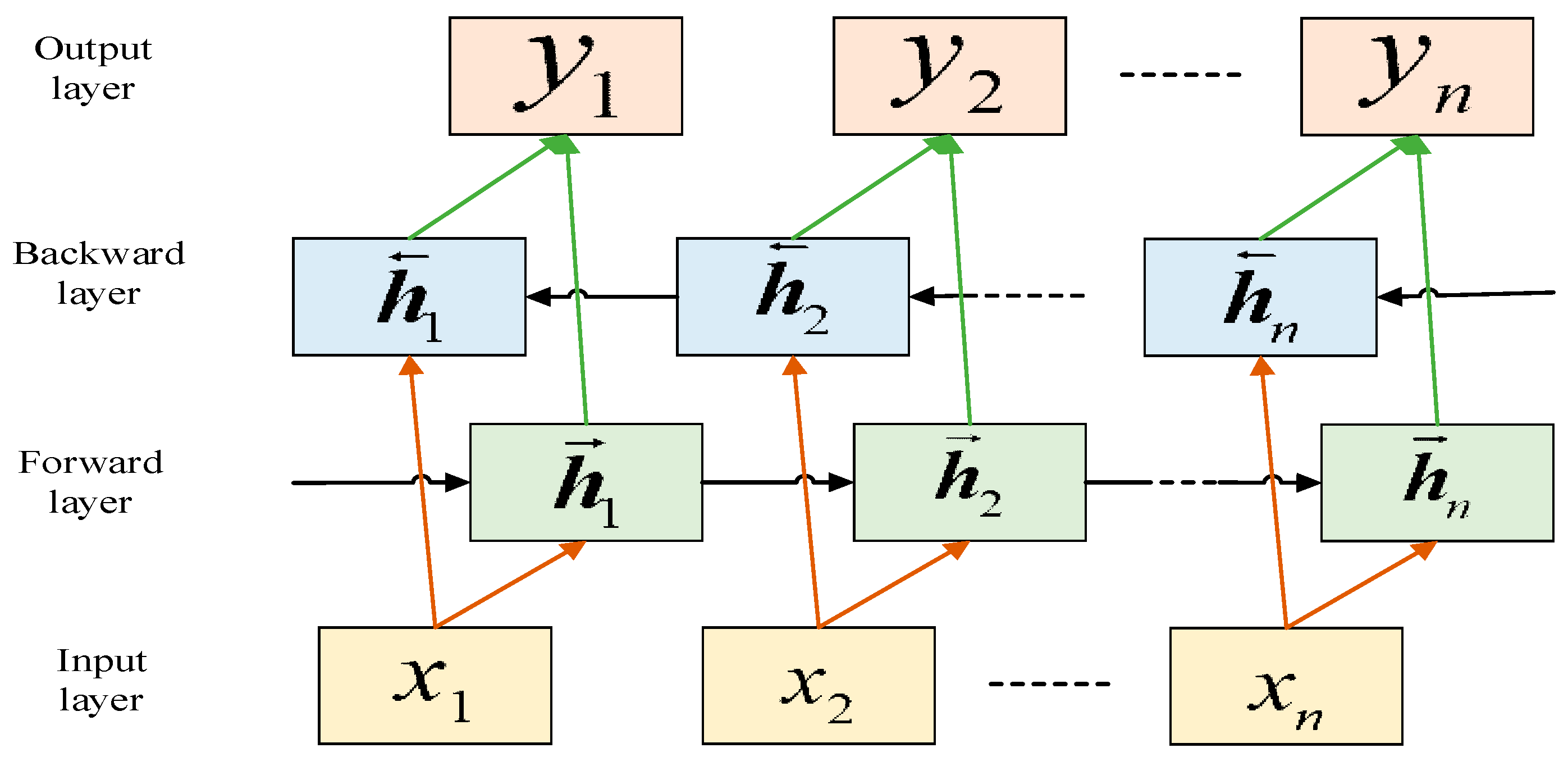
The limitation of the LSTM network unit is that it can learn the data characteristics of the preorder component but cannot combine the data characteristics of the post-order component. Bi-LSTM implements additional training by traversing the input data twice and can capture both forward and backward information. It consists of two different LSTM network hidden layers with the outputs located in opposite directions. The Bi-LSTM model is presented in Figure 2.
2.2.3. JUST-STL-Bi-LSTM Model
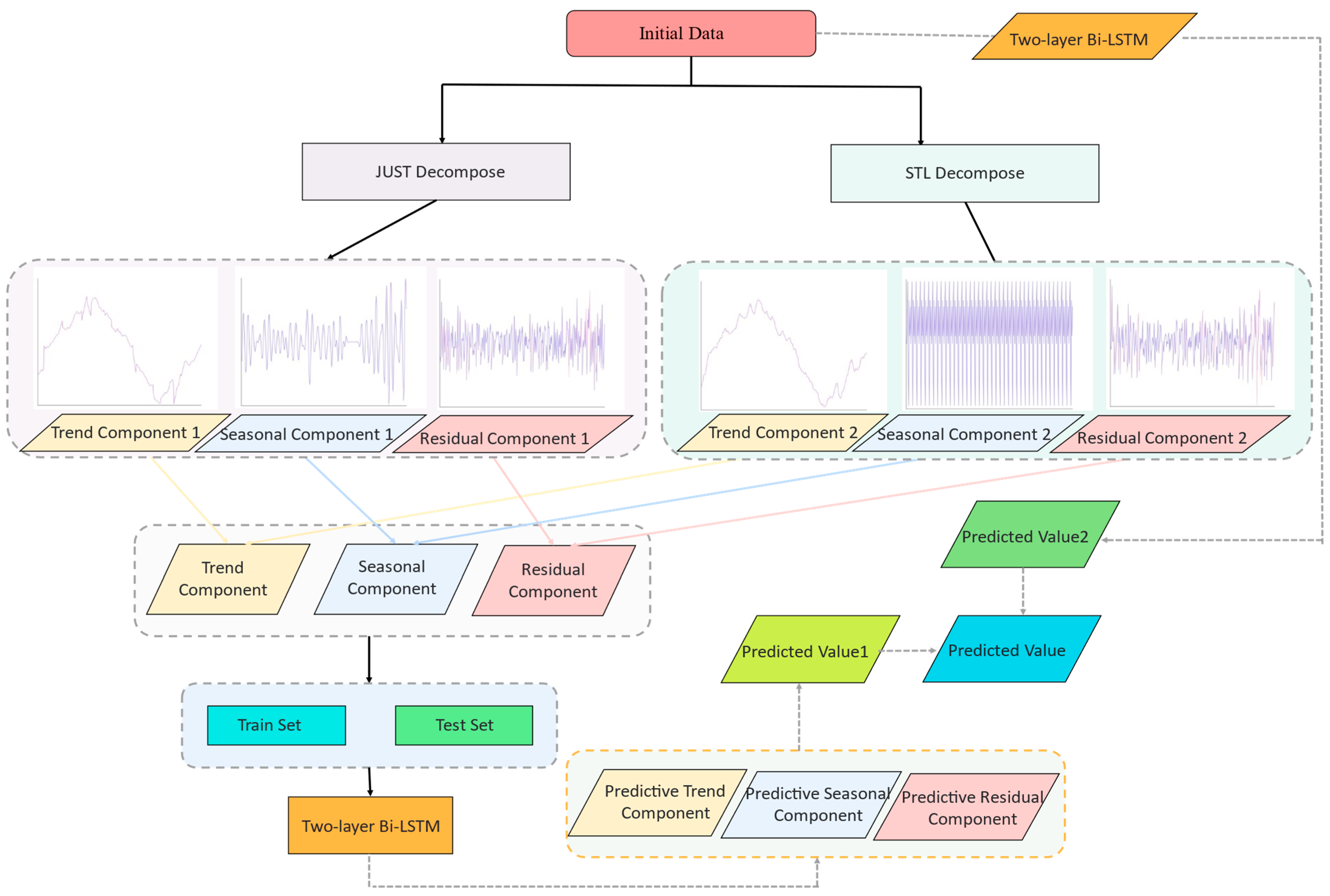
The JUST-STL-Bi-LSTM (JSBL) model is composed of two parts, namely, time-series decomposition and temperature prediction models.
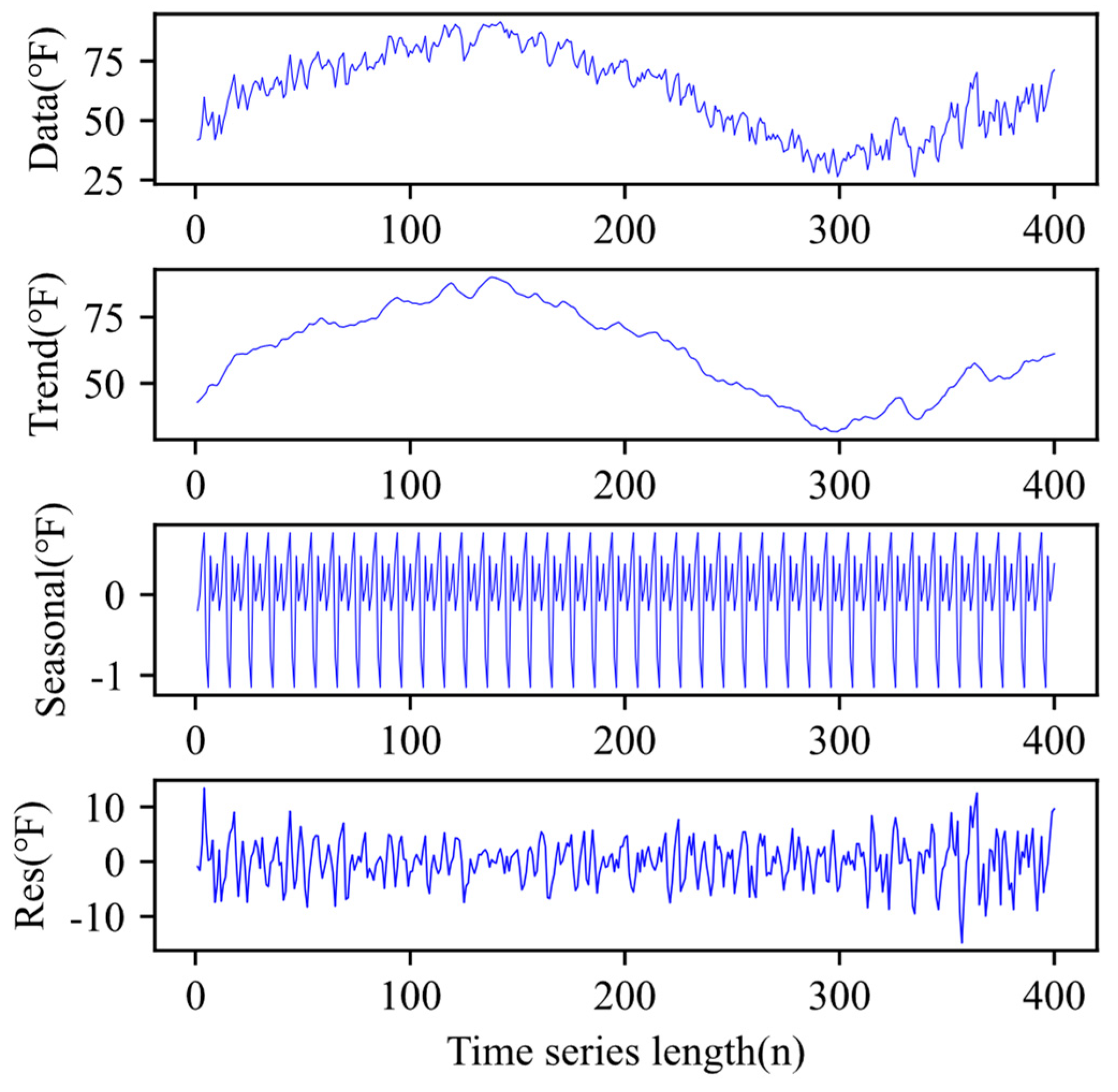
The decomposition of the temperature time-series model was performed using two methods: JUST and STL. Since the daily average temperature presents a certain periodicity, it was considered to decompose the data prior to forecasting. The prediction performed by the temperature time-series model following decomposition could effectively reduce the influence of random data fluctuations on the final prediction results. First, for the input original time-series data, the JUST decomposition algorithm was used to perform decompositions, and then trend component 1, season component 1, and residual component 1 were obtained. Then, the original time-series data were decomposed by the STL decomposition algorithm to obtain trend component 2, seasonal component 2, and residual component 2. Finally, the two sub-sequences were combined to obtain the final trend, seasonal, and residual component values. Figure 3 and Figure 4 present an example of time-series decomposition experiments using the JUST and STL networks, respectively.
The construction of the temperature prediction model contained three parts: the input, hidden, and output layers.
First, we divided the training and test sets. The data obtained from the two sets were then presented as a ratio of 9:1. Subsequently, according to the set step size, the trend, seasonal, residual components, and the original data series were indicated. In the input layer, the 4 marked time series were taken as the input values. In the hidden layer, the input data could be divided into two parts for the predictions. The first part presented the predictions made for each component. A two-layer Bi-LSTM network was used to predict the labeled trend, seasonal, and residual components. The predicted values of each component were the output through a fully connected layer, and then the obtained results were added to obtain the first predicted value. The second part included the prediction of the original temperature time series. Again, through this network, we obtained a second prediction value. Following the combination of the two predicted values, they were compressed into the final predicted value through a fully connected layer. In the output layer, the prediction sequence of the entire temperature time series was finally output. The prediction model is presented in Figure 5.
The time-series decomposition part was combined with the temperature prediction model to obtain the final flowchart, as presented in Figure 6.
3. Results
3.1. Parameter Setting
The loss function used by the model in our study was the mean square error (MSE) function. The expression of the MSE is presented as
where is the original value, is the predicted value, and is the sequence length. In the experimental model, the number of cells in the two-layer Bi-LSTM network was set to 50, and the discard rate was 0.2. The model activation function was tanh. The learning rate was 0.0001. An Adam optimizer with a rapid convergence speed was also used in the experiment. We set the batch size to 32. The step was set to 40. The ratio of the training set to test sets was 9:1. The training period was 20. The model presented in this article was tested on GeForce RTX 165 using software and modules with versions of python3.7 and keras2.3.1.
3.2. Evaluation Criteria
An adequate measurement of the model’s performance fully reveals the accuracy of the predicted results. In order to objectively evaluate the temperature prediction performance of the model proposed in this study, the root mean square error (RMSE), mean absolute error (MAE), and coefficient of determination (R2) were used as the performance measurements. The expressions of RMSE, MAE, and R2 are presented as
where represents the original value, represents the sequence mean value, represents the predicted value, and is the sequence length.
3.3. Comparison of Models
The comparison of the models included two stages: the first stage consisted of the step size experiment, for which the purpose was to elect the appropriate step size value according to the experimental results; the second stage consisted of testing the predictive power of the model using additional test data after the step size was fixed. Comparative experiments were conducted on the Bi-LSTM, EMD-LSTM, STL-LSTM, and JUST-STL-Bi-LSTM models. JSBL represents the JUST-STL-Bi-LSTM model proposed in this paper. The step size experiment included a dataset of the daily mean temperature levels of 34 provincial capital cities in China.
3.3.1. Step Size Experiment
When the step size values were set to 20, 30, and 40, the RMSE values of the four models with different step sizes were obtained, as shown in Table 1. The RMSE value of the JSBL model was 0.2187 when the step size was 40. The values obtained for the other models were 4.3997, 2.5343, and 0.9336. We can observe that the RMSE result for the JSBL model is minimal.
As can be observed in Table 1, the prediction accuracy of the model combined with the decomposition algorithm is significantly higher than that of the model lacking a decomposition algorithm, indicating that the combination of an appropriate decomposition algorithm can effectively improve the prediction accuracy of the algorithm. It can also be observed in Table 1 that the prediction accuracy of the Bi-LSTM model changes a little when the step size is different. The accuracy of the STL-LSTM model and the model presented in this paper produced the best results when the step size was 40.
The MAEs of the four models with different step sizes are presented in Table 2. According to Table 2, the MAE of each model changes little when the step sizes are 20 and 30, and the JSBL model presents the best MAE when the step size is 40. R2 is presented in Table 3. For a smaller step size, JSBL combined the JUST and STL algorithms, which needed to learn more features, the model training process was slower, and some features had not been learned at the end of the cycle. Therefore, the prediction accuracy of the JSBL model may be reduced when incorporating smaller step sizes. In contrast, the STL-LSTM model needs to learn fewer features, and a smaller step size can satisfy the training demand; a continuous increase in the step size instead leads to the occurrence of scattering or oscillation in the model’s training process.
From the observation of Table 1, Table 2 and Table 3, it can be determined that when the step size is 40, the performance of the algorithm proposed in this paper is successfully reflected, and other models also perform well when incorporating this step size. Therefore, the step size of 40 was selected to conduct subsequent model evaluation experiments.
3.3.2. Model Evaluation
In the model evaluation experiment, the daily mean temperature dataset of 60 random cities located in China was used. The model evaluation experiment consisted of four stages. Firstly, each model was evaluated using the evaluation metrics for the dataset. Secondly, in order to test the sensitivity of the model to the data, the evaluation indexes of each model were tested using the cumulative distribution function. Thirdly, in order to display the intuitive prediction effect of the model, a longer length of data was randomly selected to display the prediction effect of the model. Finally, in order to successfully present the differences in the prediction’s details, the data with lengths of 60 were selected to compare the prediction effects of each model.
Several models were evaluated using additional daily mean temperature datasets to test the predictive power of the models. For our convenience, numbers 1–60 were used in this study to indicate the corresponding site of each city. For the changes in the R2 values in the additional test dataset, only the changes in 10 random sites were presented in this study, as shown in Table 4. It can be observed in Table 4 that the R2 values for all models were higher than 0.9, which indicates that all the models had a certain ability to perform predictions. Secondly, the JUST-STL-Bi-LSTM (JSBL) model presented the highest fitting coefficient, indicating that it attained the best fitting degree.
The RMSE and MAE values of the four models on the additional test datasets are presented in Figure 7 and Figure 8, respectively.
The following information can be observed in Figure 7 and Figure 8. Firstly, the RMSE and MAE values of the model presented in this paper are both the lowest. Secondly, the RMSE and MAE values of the JUST-STL-Bi-LSTM and STL-LSTM models fluctuate, almost in the shape of a horizontal line, and present strong resistance to sensitive data. However, the Bi-LSTM and EMD-LSTM models presented a wide fluctuation range and high sensitivity to the data. Therefore, the model proposed in this paper was superior to the other models in its ability to perform predictions.
The average performance indexes of several models on additional test datasets were calculated during the experiment, including the RMSE, R2, and MAE. The JSBL model performed the best on the additional 60-site test datasets, followed by the STL-LSTM, EMD-LSTM, and Bi-LSTM models. The average RMSE, MAE, and R2 values of each model are presented in Table 5.
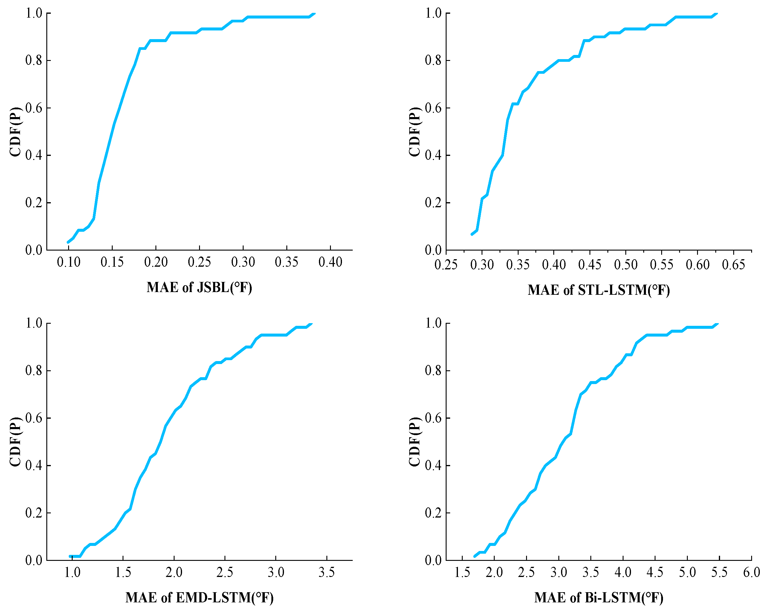
The average RMSE and MAE values only reflected the comprehensive performance of the model; however, they could not present the sensitivity of the model to the data. In order to present the sensitivity of several models to the data, the cumulative distribution function (CDF) was used to calculate the distributions of the RMSE and MAE values. The cumulative distribution function is defined as Formula (12), where represents the real variables, is the probability distribution of all values, and represents the probability. The cumulative distribution function is defined as the sum of the probabilities of all variables less than or equal to .
This study conducted a CDF analysis on both RMSE and MAE. Figure 9 presents the CDF changes presented the RMSEs of the four models. By observing Figure 9, it can be determined that most of the errors produced by the JSBL model are concentrated less than a value of 0.4, where the probability is very close to 100%, indicating that most of the errors exhibited are less than 0.4. This result indicates that, for most of the data obtained, the prediction errors produced by the model are close, the sensitivity to the data is not high, and the adaptability is good. For the STL-LSTM model, concerning all the error data, the majority of the errors were less than a value of 0.75. For the remaining two models, the CDF curve changed more uniformly, indicating that the error distribution in the error dataset was more evenly distributed. The proportion of smaller and greater errors was close, indicating that the model was highly sensitive to the input data. Figure 10 presents the CDF changes observed for the MAEs of the four models.
The Kolmogorov–Smirnov predictive accuracy (KSPA) method can accurately test whether a statistically significant difference between the prediction errors of the two models is present [33,34]. We used KSPA to test whether the prediction errors produced by the JSBL model were statistically significantly different from those produced by the other models. We attained statistics for the RMSE values only. The -value of the two-sided KSPA test was less than 0.05, indicating that there was a statistically significant difference evident between the prediction errors produced by the two models. The -value of the one-sided KSPA test was less than 0.05, indicating that the JSBL model produced a lower random error value than the other models. The test results are presented in Table 6. -values less than 0.05 refer to the 95% confidence level. As can be observed in Table 6, all the -values are within the 95% confidence level range, indicating that our model produced a lower random error than the other models.
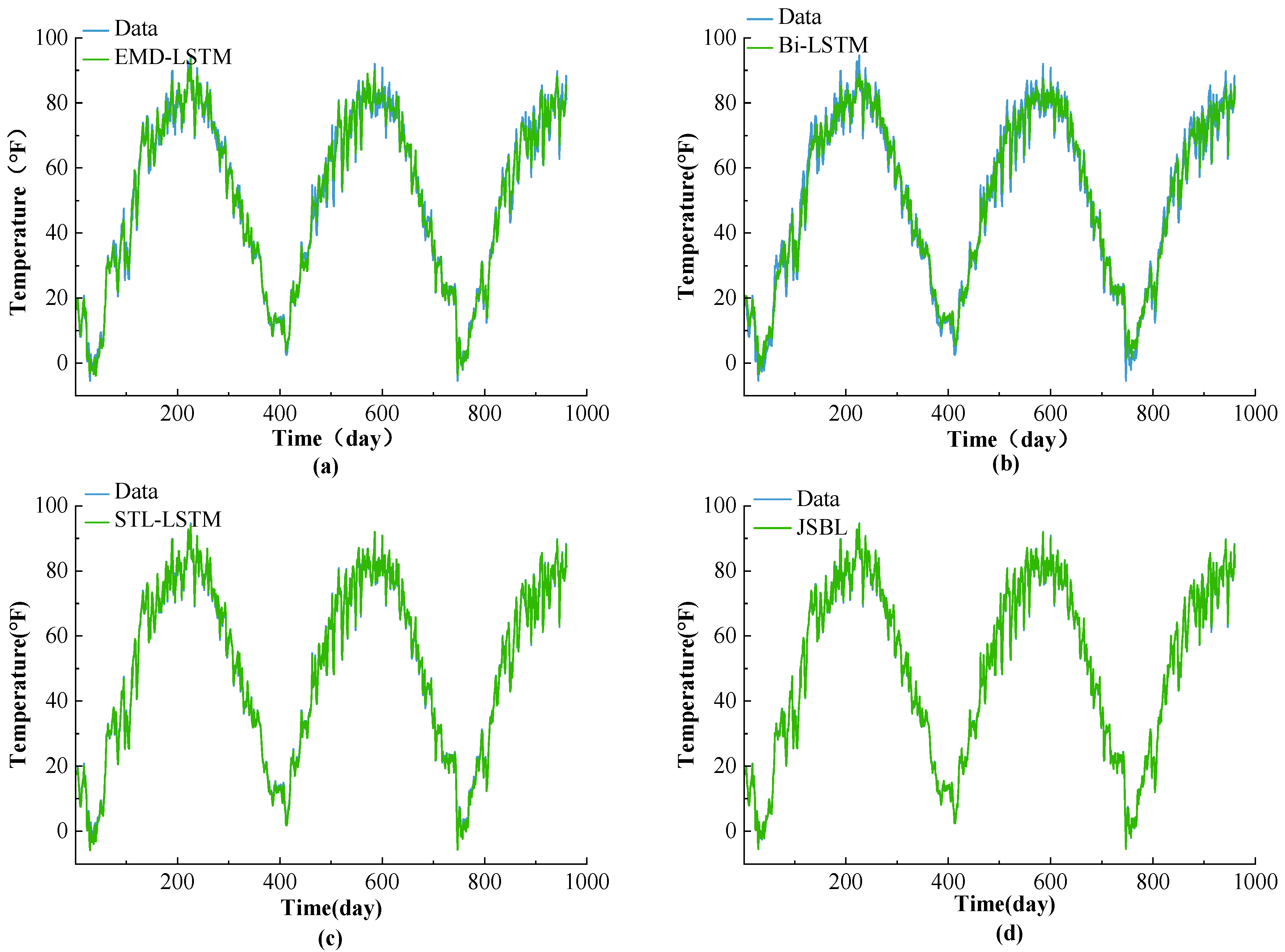
To accurately display the prediction effect of each model, the test data with a sequence length of 960 days were randomly selected to perform a comparison, as shown in Figure 11. In Figure 11, it can be observed that the Bi-LSTM and EMD-LSTM models produce poor prediction effects. A considerable error between the real and predicted values for this model is evident. The JSBL and STL-LSTM models presented prediction effects. The error evident between the predicted and true values is small. At the same time, it can be observed that the JSBL model forecasted the relevant details more appropriately than the STL-LSTM model. The results show that the JSBL model has better practicability and effectiveness characteristics.
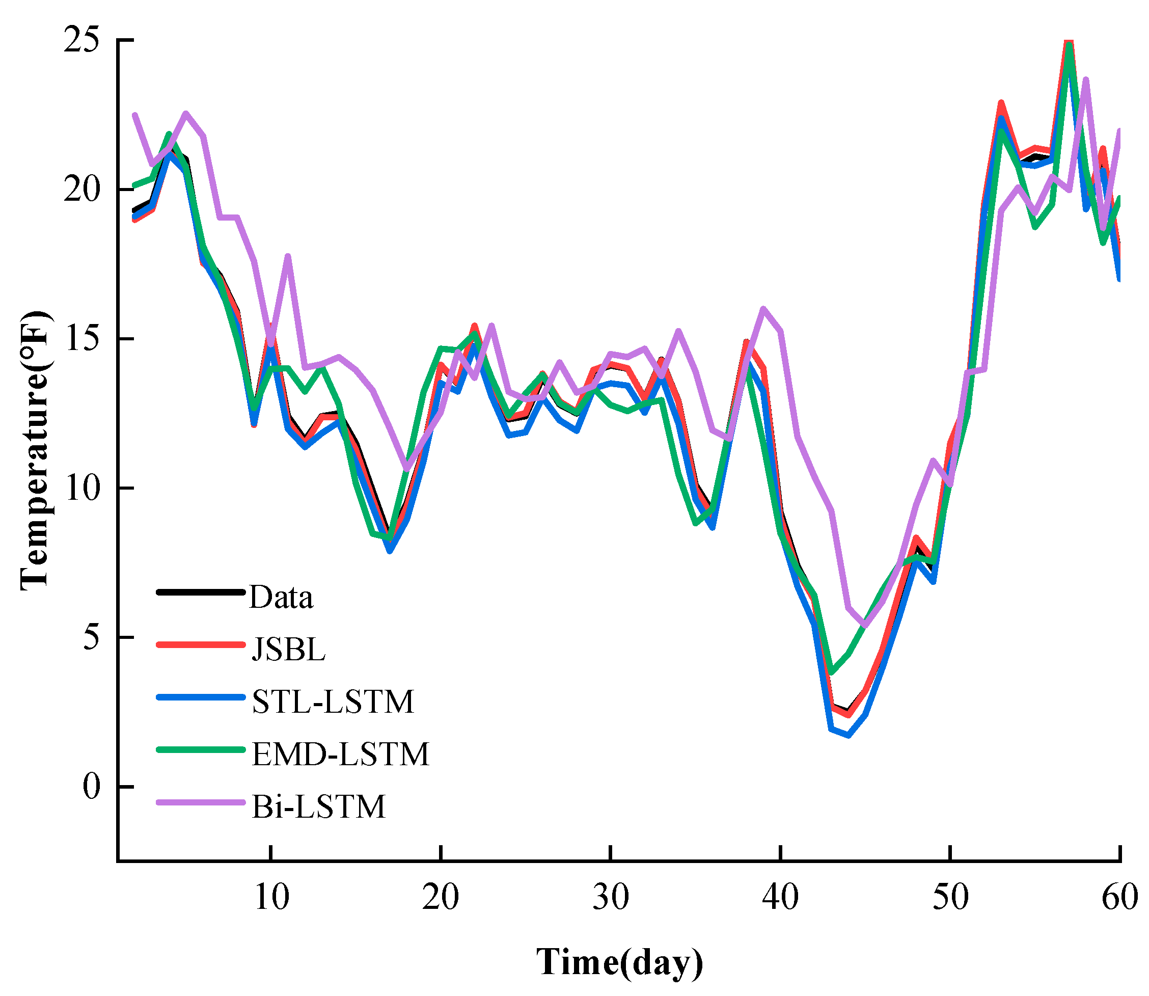
In order to present the prediction results for each model, the data with a time length of 60 days were randomly selected for a post-prediction comparison. As shown in Figure 12, we can observe that the JSBL model is much better at predicting the relevant details. The predicted value is much closer to the true value. The JSBL, STL-LSTM, and EMD-LSTM models present light hysteresis, while the Bi-LSTM model presents strong hysteresis. Then, the predictions of the STL-LSTM, EMD-LSTM, and Bi-LSTM models successively declined in their accuracy.
4. Discussion and Conclusions
In this study, we proposed a temperature prediction model based on time-series decomposition and Bi-LSTM neural networks. Our model effectively reduced the influence of random fluctuations occurring in the temperature data on the prediction results and presented accurate daily average temperature level predictions for cities located in China. The prediction results show that our model has greater prediction accuracy characteristics than the Bi-LSTM model without the time-series decomposition method. Compared to the EMD-LSTM and STL-LSTM models and combined with the time-series decomposition algorithm, the predicted results are also closer to the actual curve presented and achieved better data anti-sensitivity results. For several evaluation indicators, our model performed the best.
In this study, the relevant network was first optimized through the step size experiment, and the final step size value was set by including different step sizes and comparing the evaluation indexes for each step size. Secondly, the predictive ability of each model was tested by randomly selected additional test datasets. Thirdly, in order to display the data anti-sensitivity values of each model, the cumulative distribution function was used to calculate the distribution probability of each evaluation index in the experiment. The results show that the JSBL model has the strongest anti-sensitive data characteristic. Finally, in order to successfully display the intuitive prediction effect, this study randomly selected the data collected from additional test sets and used several models to perform the predictions. From the intuitive prediction effect, it can be observed that our model and the STL-LSTM model presented better prediction effects, and the predicted value was closer to the real value.
The model proposed in this paper presented better prediction accuracy, rapid convergence, the ability to learn the appropriate data features rapidly, and stronger data-resistance sensitivity. The limitation of JSBL is that the model is based on univariate temperature time series, and the model of multi-variable temperature time series requires further study in the field. On the basis of the research presented in this paper, we aim to pursue the following research directions: for multi-variable time series, feature extraction should be conducted by combining a convolutional neural network with our model to further optimize its performance.
Author Contributions
Conceptualization, X.H.; methodology, X.H. and K.S.; validation, K.Z.; writing—original draft preparation, K.Z.; writing—review and editing, K.Z.; funding acquisition, X.H. All authors have read and agreed to the published version of the manuscript.
Funding
This research was funded by the National Natural Science Foundation of China, grant number 61872407.
Data Availability Statement
The data presented in this study are available upon request from the corresponding author.
Conflicts of Interest
The authors declare no conflict of interest.
References
- DeFries, R.S.; Field, C.B.; Fung, I.; Collatz, G.J.; Bounoua, L. Combining satellite data and biogeochemical models to estimate global effects of human-induced land cover change on carbon emissions and primary productivity. Glob. Biogeochem. Cycles 1999, 13, 803–815. [Google Scholar] [CrossRef]
- Luo, L.F.; Wood, E.F. Monitoring and predicting the 2007 U.S. drought. Geophys. Res. Lett. 2007, 34, L22702. [Google Scholar] [CrossRef]
- Farjad, B.; Gupta, A.; Sartipizadeh, H.; Cannon, A.J. A novel approach for selecting extreme climate change scenarios for climate change impact studies. Sci. Total Environ. 2019, 678, 476–485. [Google Scholar] [CrossRef] [PubMed]
- Akther, M.S.; Hassan, Q.K. Remote Sensing-Based Assessment of Fire Danger Conditions Over Boreal Forest. IEEE J. Sel. Top. Appl. Earth Obs. Remote Sens. 2011, 4, 992–999. [Google Scholar] [CrossRef]
- Gabriel, T.R.; André, A.P.S.; Viviana, C.M.; Leandro, S.C. Novel hybrid model based on echo state neural network applied to the prediction of stock price return volatility. Expert Syst. Appl. 2021, 184, 115490. [Google Scholar] [CrossRef]
- Contreras, J.; Espinola, R.; Nogales, F.J.; Conejo, A.J. ARIMA models to predict next-day electricity prices. IEEE Power Eng. Rev. 2002, 22, 57. [Google Scholar] [CrossRef]
- Ugurlu, U.; Oksuz, I.; Tas, O. Electricity Price Forecasting Using Recurrent Neural Networks. Energies 2018, 11, 1255. [Google Scholar] [CrossRef]
- Behera, R.K.; Das, S.; Rath, S.K.; Damasevicius, R. Comparative study of real time machine learning models for stock prediction through streaming data. J. Univ. Comput. Sci. 2020, 26, 1128–1147. [Google Scholar] [CrossRef]
- Chimmula, V.K.R.; Zhang, L. Time Series Forecasting of COVID-19 transmission in Canada Using LSTM Networks. Chaos Solitons Fractals 2020, 135, 109864. [Google Scholar] [CrossRef]
- Zhang, J.; Jiang, Z. A new grey quadratic polynomial model and its application in the COVID-19 in China. Sci. Rep. 2021, 11, 12588. [Google Scholar] [CrossRef] [PubMed]
- Shekhawat, S.; Saxena, A.; Zeineldin, R.A.; Mohamed, A.W. Prediction of Infectious Disease to Reduce the Computation Stress on Medical and Health Care Facilitators. Mathematics 2023, 11, 490. [Google Scholar] [CrossRef]
- Burke, M.; Hsiang, S.M.; Miguel, E. Global non-linear effect of temperature on economic production. Nature 2015, 527, 235–239. [Google Scholar] [CrossRef] [PubMed]
- Nunes, A.R. General and specified vulnerability to extreme temperatures among older adults. Int. J. Environ. Health Res. 2020, 30, 515–532. [Google Scholar] [CrossRef]
- Chen, J.L.; Li, G.; Wu, D.C.; Shen, S. Forecasting seasonal tourism demand using a multiseries structural time series method. J. Travel Res. 2019, 58, 92–103. [Google Scholar] [CrossRef]
- Ahmadi, F.; Nazeri Tahroudi, M.; Mirabbasi, R.; Khalili, K.; Jhajharia, D. Spatiotemporal trend and abrupt change analysis of temperature in Iran. Meteorol. Appl. 2018, 25, 314–321. [Google Scholar] [CrossRef]
- Meshram, S.G.; Kahya, E.; Meshram, C.; Ghorbani, M.A.; Ambade, B.; Mirabbasi, R. Long-term temperature trend analysis associated with agriculture crops. Theor. Appl. Climatol. 2020, 140, 1139–1159. [Google Scholar] [CrossRef]
- Shi, X.; Huang, Q.; Chang, J.; Wang, Y. Optimal parameters of the SVM for temperature prediction. Proc. Int. Assoc. Hydrol. Sci. 2015, 368, 162–167. [Google Scholar] [CrossRef]
- Chen, X.; Xu, A. Temperature and humidity of air in mine roadways prediction based on BP neural network. In Proceedings of the 2011 International Conference on Multimedia Technology, Hangzhou, China, 26–28 July 2011. [Google Scholar]
- Wang, X.W.; Wang, X.L.; Wang, L.; Jiang, L.J.; Zhan, Y.J. A distributed fusion LSTM model to forecast temperature and relative humidity in smart buildings. In Proceedings of the 16th IEEE Conference on Industrial Electronics and Applications, Chengdu, China, 1–4 August 2021. [Google Scholar]
- Jiang, Y.; Zhao, M.; Zhao, W.; Qin, H.; Qi, H.; Wang, K.; Wang, C. Prediction of sea temperature using temporal convolutional network and LSTM-GRU network. Complex Eng. Syst. 2021, 1, 6. [Google Scholar] [CrossRef]
- Yan, B.J.; Tang, X.Y.; Liu, B.Y.; Wang, J.; Zhou, Y.Z.; Zheng, G.P.; Zou, Q.; Lu, Y.; Tu, W.X. An improved method for the fitting and prediction of the number of COVID-19 confirmed cases based on LSTM. CMC-Comput. Mater. Contin. 2020, 64, 1473–1490. [Google Scholar] [CrossRef]
- Zhang, B.; Wang, H.; Jiang, L.; Yuan, S.; Li, M. A novel bidirectional lstm and attention mechanism based neural network for answer selection in community question answering. Comput. Mater. Contin. 2020, 62, 1273–1288. [Google Scholar] [CrossRef]
- Hassani, H.; Zhigljavsky, A. Singular spectrum analysis: Methodology and application to economics data. J. Syst. Sci. Complex. 2009, 22, 372–394. [Google Scholar] [CrossRef]
- Huo, Y.H.; Yan, Y.; Du, D.; Wang, Z.H.; Zhang, Y.X.; Yang, Y. Long-Term span traffic prediction model based on STL decomposition and LSTM. In Proceedings of the 2019 20th Asia-Pacific Network Operations and Management Symposium, Matsue, Japan, 18–20 September 2019. [Google Scholar]
- Chen, D.; Zhang, J.; Jiang, S. Forecasting the short-term metro ridership with seasonal and trend decomposition using loess and LSTM neural networks. IEEE Access 2020, 8, 91181–91187. [Google Scholar] [CrossRef]
- Chen, Q.; Wen, D.; Li, X.; Chen, D.; Lv, H.; Zhang, J.; Gao, P. Empirical mode decomposition based long short-term memory neural network forecasting model for the short-term metro passenger flow. PLoS ONE 2019, 14, e0222365. [Google Scholar] [CrossRef] [PubMed]
- Yin, H.; Jin, D.; Gu, Y.H.; Park, C.J.; Han, S.K.; Yoo, S.J. STL-ATTLSTM: Vegetable price forecasting using STL and attention mechanism-based LSTM. Agriculture 2020, 10, 612. [Google Scholar] [CrossRef]
- National Climatic Data Center; NESDIS; NOAA; U.S. Department of Commerce. Global Summary of the Day. 2022. Available online: https://www.ncei.noaa.gov/maps/alltimes/ (accessed on 1 September 2022).
- Ghaderpour, E.; Vujadinovic, T. Change Detection within Remotely Sensed Satellite Image Time Series via Spectral Analysis. Remote Sens. 2020, 12, 4001. [Google Scholar] [CrossRef]
- Ghaderpour, E.; Liao, W.; Lamoureux, M. Antileakage least-squares spectral analysis for seismic data regularization and random noise attenuation. Geophysics 2018, 83, V157–V170. [Google Scholar] [CrossRef]
- Jallal, M.A.; Chabaa, S.; Yassini, A.; Zeroual, A.; Ibnyaich, S. Air temperature forecasting using artificial neural networks with delayed exogenous input. In Proceedings of the International Conference on Wireless Technologies, Embedded and Intelligent Systems, Fez, Morocco, 3–4 April 2019. [Google Scholar]
- Hochreiter, S.; Schmidhuber, J. Long Short-Term Memory. Neural Comput. 1997, 9, 1735–1780. [Google Scholar] [CrossRef]
- Hassani, H.; Heravi, S.; Zhigljavsky, A. Forecasting UK industrial production with multivariate Singular Spectrum Analysis. J. Forecast. 2013, 32, 395–408. [Google Scholar] [CrossRef]
- Hassani, H.; Silva, E. A Kolmogorov-Smirnov Based Test for Comparing the Predictive Accuracy of Two Sets of Forecasts. Econometrics 2015, 3, 590–609. [Google Scholar] [CrossRef]
Figure 1.
The structure of the LSTM network.

Figure 2.
The structure of the Bi-LSTM model.

Figure 3.
The JUST method decomposing the time-series data.

Figure 4.
The STL method decomposing the time-series data.

Figure 5.
The temperature prediction model.

Figure 6.
The JUST-STL-Bi-LSTM model.

Figure 7.
RMSE values of four models on the test dataset.

Figure 8.
MAE values of four models on the test dataset.

Figure 9.
CDF changes in RMSE values.

Figure 10.
CDF changes in MAE values.

Figure 11.
(a) Prediction results for the EMD-LSTM; (b) Bi-LSTM; (c) STL-LSTM; and (d) JSBL models.

Figure 12.
Comparison of the predictions performed by the four models.


Table 1.
RMSE values for four models with different step size values.
| Model | 20 | 30 | 40 |
|---|---|---|---|
| JSBL | 0.7087 | 0.4996 | 0.2187 |
| Bi-LSTM | 4.4173 | 4.3340 | 4.3997 |
| EMD-LSTM | 2.6376 | 2.6279 | 2.5343 |
| STL-LSTM | 0.6583 | 1.0882 | 0.9336 |
Table 2.
MAE values of four models with different step sizes.
| Model | 20 | 30 | 40 |
|---|---|---|---|
| JSBL | 0.6563 | 0.4735 | 0.1737 |
| Bi-LSTM | 3.3478 | 3.2760 | 3.3349 |
| EMD-LSTM | 2.0575 | 2.0209 | 1.9265 |
| STL-LSTM | 0.5194 | 0.4785 | 0.7066 |
Table 3.
R2 values of four models with different step sizes.
| Model | 20 | 30 | 40 |
|---|---|---|---|
| JSBL | 0.9981 | 0.9990 | 0.9999 |
| Bi-LSTM | 0.9286 | 0.9302 | 0.9271 |
| EMD-LSTM | 0.9741 | 0.9743 | 0.9758 |
| STL-LSTM | 0.9984 | 0.9956 | 0.9967 |
Table 4.
R2 value comparisons of four models.
| Site | JSBL | Bi-LSTM | EMD-LSTM | STL-LSTM |
|---|---|---|---|---|
| 1 | 0.9999 | 0.9285 | 0.9722 | 0.9977 |
| 2 | 0.9996 | 0.8904 | 0.9600 | 0.9980 |
| 3 | 0.9999 | 0.9530 | 0.9817 | 0.9995 |
| 4 | 0.9999 | 0.9552 | 0.9825 | 0.9995 |
| 5 | 0.9999 | 0.9567 | 0.9838 | 0.9996 |
| 6 | 0.9999 | 0.9474 | 0.9749 | 0.9991 |
| 7 | 0.9999 | 0.9369 | 0.9732 | 0.9992 |
| 8 | 0.9997 | 0.8840 | 0.9639 | 0.9981 |
| 9 | 0.9998 | 0.9217 | 0.9724 | 0.9971 |
| 10 | 0.9998 | 0.9326 | 0.9778 | 0.9991 |
Table 5.
The average R2, RMSE, and MAE values of the four models.
| Model | R2 | RMSE | MAE |
|---|---|---|---|
| JSBL | 0.9998 | 0.2146 | 0.1616 |
| Bi-LSTM | 0.9306 | 4.0754 | 3.0961 |
| EMD-LSTM | 0.9742 | 2.5455 | 1.9363 |
| STL-LSTM | 0.9986 | 0.4887 | 0.3594 |
Table 6.
The KSPA test.
| Test | JSBL and STL-LSTM | JSBL and EMD-LSTM | JSBL and Bi-LSTM |
|---|---|---|---|
| Two-sided (-value) | 4.441 × 10⁻¹⁶ | 4.441 × 10⁻¹⁶ | 4.441 × 10⁻¹⁶ |
| One-sided (-value) | 2.2 × 10⁻¹⁶ | 2.2 × 10⁻¹⁶ | 2.2 × 10⁻¹⁶ |
Disclaimer/Publisher’s Note: The statements, opinions and data contained in all publications are solely those of the individual author(s) and contributor(s) and not of MDPI and/or the editor(s). MDPI and/or the editor(s) disclaim responsibility for any injury to people or property resulting from any ideas, methods, instructions or products referred to in the content. |
© 2023 by the authors. Licensee MDPI, Basel, Switzerland. This article is an open access article distributed under the terms and conditions of the Creative Commons Attribution (CC BY) license (https://creativecommons.org/licenses/by/4.0/).
Share and Cite
MDPI and ACS Style
Zhang, K.; Huo, X.; Shao, K. Temperature Time Series Prediction Model Based on Time Series Decomposition and Bi-LSTM Network. Mathematics 2023, 11, 2060. https://0-doi-org.brum.beds.ac.uk/10.3390/math11092060
AMA Style
Zhang K, Huo X, Shao K. Temperature Time Series Prediction Model Based on Time Series Decomposition and Bi-LSTM Network. Mathematics. 2023; 11(9):2060. https://0-doi-org.brum.beds.ac.uk/10.3390/math11092060
Chicago/Turabian StyleZhang, Kun, Xing Huo, and Kun Shao. 2023. "Temperature Time Series Prediction Model Based on Time Series Decomposition and Bi-LSTM Network" Mathematics 11, no. 9: 2060. https://0-doi-org.brum.beds.ac.uk/10.3390/math11092060
Note that from the first issue of 2016, this journal uses article numbers instead of page numbers. See further details here.