Article

Guaranteed H∞ Performance of Switched Systems with State Delays: A Novel Low-Conservative Constrained Model Predictive Control Strategy

by
Yasser Falah Hassan
1,
Mahmood Khalid Hadi Zarkani
1,
Mohammed Jasim Alali
1,
Haitham Daealhaq
1 and
Hicham Chaoui
2,3,*
1
College of Engineering, University of Kerbala, Karbala 56001, Iraq
2
Faculty of Engineering and Design, Carleton University, Ottawa, ON K1S 5B6, Canada
3
College of Engineering, Texas Tech University, Lubbock, TX 79409, USA
*
Author to whom correspondence should be addressed.
Submission received: 6 November 2023 / Revised: 23 December 2023 / Accepted: 4 January 2024 / Published: 11 January 2024
(This article belongs to the Special Issue Advances in Dynamical System Modelling and Computer-Aided Design)

Abstract

:
In this paper, for the first time, a simultaneous design of a model predictive control plan and persistent dwell-time switching signal utilizing the conventional multiple Lyapunov–Krasovskii functional is proposed for linear delayed switched systems that are affected by physical constraints and exogenous disturbances. The conventional multiple Lyapunov–Krasovskii functional with a ‘jump high’ condition is used as a step forward to reduce the strictness of constraints on controller design compared with the switched Lyapunov–Krasovskii functional. However, a dwell-time constraint is inflicted on the switching signal by the ‘jump-high’ condition. Therefore, to decrease the dwell-time limit, the persistent dwell-time structure is used and compared with other structures. Also, a new online framework is proposed to reduce the number of constraints on controller design at each time step. Moreover, for the first time, exogenous disturbances are considered in the procedure of MPC design for delayed switched systems, and non-weighted H∞ performance is ensured. The simulation outcome demonstrates the great performance of the suggested plan and its ability to asymptotically stabilize the switched system.

1. Introduction

Switched systems, which are a key branch of hybrid systems and contain two levels, have received a lot of attention in recent years, especially on the topic of control. A group of sub-systems expressed with differential equations form the lower level, and the active sub-system is characterized by the higher level [1]. In practice, systems are exposed to various factors such as permanent and intermittent faults or structural changes, which can explain the complex behavior of these systems with the structure of switched systems. Network control systems and drinking water supply networks are examples of systems that are affected by permanent and intermittent faults and structural changes, which can be modeled as switched systems. On the other hand, systems such as wind turbines and satellites, which are in the category of complex nonlinear systems, can be divided into many dynamics by specifying switching boundaries. Therefore, according to the discussed topics, it is important to examine the challenges of switched systems [2,3,4].
One of the most important and challenging concerns in switched systems is ensuring their overall stability. The stability problem of switched systems includes several interesting phenomena. For example, it is possible for a switched system to become unstable for special switching signals when all sub-systems are exponentially stable. Also, all sub-systems may be unstable, but certain switching signals stabilize them [5]. Therefore, the stability problem of switched systems can be divided into three types. The first type is related to the analysis of stability based on a prescribed switching signal [6]. The second type is related to the analysis of stability based on an arbitrary switching signal [7], and the third type is related to the analysis of stability based on a restricted switching signal [8]. In switched systems, the prescribed switched system may exist, that is, switching moments and active intervals for each of the systems are given. Thus, the stability analysis is performed based on this planned signal that results in the reduction in conservatism [9]. If no constraint on the switching signal is considered in the stability analysis, the problem is known as a stability analysis under arbitrary switching signals [10]. A necessary condition for this problem is the asymptotic stability of all sub-systems. However, it is possible that when all sub-systems are exponentially stable, the switched system is not stable under any switching signal. Thus, two important tools, including the common Lyapunov function and the switched Lyapunov function, are introduced, which provide sufficient conditions for stability under arbitrary switching [11]. If there is no common Lyapunov function (CLF) and switched Lyapunov function (SLF) for the switched system, it is not possible to analyze its stability under any switching signal. Thus, the multiple Lyapunov function (MLF) is introduced. By using the MLF, the restricted switching signal is designed. Restricted switching signals may naturally result from the physical constraints of the system. Also, there are cases where a person has knowledge about the probable switching of the system, which causes constraints in the switching laws. With such knowledge, more powerful stability results are achieved than with arbitrary switching. The switching law may have time-dependent limitations (such as a constant dwell-time (DT), average dwell-time (ADT), and persistent dwell-time (PDT)) [12] or may have state-dependent limitations [13]. A state-dependent switching signal may exist inherently in the switched system. For example, in piecewise affine and piecewise linear systems, each region of state space has its own differential equations, and by moving from one region to another, the switching happens inherently [14]. Moreover, in some switched systems, these types of signals can be designed in such a way that regions and switching borders are specified [15]. A time-dependent switching law provides the possibility of absorbing the increased energy at switching moments using the stable sub-systems by creating a time compromise among the sub-systems [16]. Therefore, the stability of the switched system can be guaranteed. Time-dependent switching signals are of interest due to the development of various types of them and giving the decision parameters [17].
How to control and optimize the performance of switched systems is another important challenge that should be paid attention to. There have been many investigations related to the control of switched systems from the past until now, such as those conducted in [18,19,20,21,22,23,24,25,26,27]. However, one of the popular control strategies that has received less attention in switched systems is model predictive control (MPC). The model predictive controller is an online and optimal controller that can counteract the physical limitations of a system. A number of research works in the field of the MPC scheme have been developed for switched systems without considering a delay structure [28,29,30,31]. In [28,29], the switching signal was considered arbitrary, and the MPC schemes were extended using SLF. Therefore, these schemes are conservative or may not be feasible for a wide range of switched systems. In other words, they impose strict conditions on controller design and may not find a suitable control gain. In [30,31], the switching signal was considered time-dependent with an ADT structure, and the MPC schemes were extended using the MLF. These schemes partially addressed the problem of conservatism but did not take into account the physical limitations of the system or the effects of exogenous disturbances. MPC schemes have been investigated very little in previous studies on delayed switched systems [32,33]. These studies extended MPC schemes with arbitrary switching signals using a switched Lyapunov–Krasovskii functional (SLKF), which led to a set of strict constraints or infeasibility constraints on controller design for a wide range of switched systems. Also, they are not applicable for switched systems subjected to physical limitations and exogenous disturbances.
In non-MPC schemes, many efforts have been made to reduce conservatism in the design process of delayed switched systems. The works conducted in [34,35,36], the most recent works, presented a strict decreasing LKF, which led to the elimination of the ‘jump high’ condition and relaxation of the dwell-time constraints. However, in MPC schemes for delayed switched systems, the conventional MLKF with a ‘jump high’ condition has not yet been used as a step forward to reduce conservatism compared with the SLKF. Also, in this paper, by presenting a new online framework, the conservatism caused by this condition is reduced. Therefore, the first motivation of this study was the design of an MPC scheme using the conventional MLKF with a new online framework to reduce the strictness of constraints on the controller design compared with other MPC schemes extended using the SLKF. In this new online framework, the ‘jump high’ condition is applied only at the switching instant and only based on the current transition between two sub-systems. In fact, it is not necessary for the ‘jump high’ conditions to be applied based on all transitions among sub-systems at all time steps, and, consequently, the conservatism decreases. It should also be noted that a dwell-time constraint is applied to the switching signal by the “jump-high” condition. Therefore, the second goal of this research was to attenuate the dwell-time constraint compared with other structures via the concurrent design of MPC and switching with the PDT structure. Another advantage of this new online framework is that at each step time, only the constraints related to the active sub-system are applied. Therefore, it is not necessary to apply the constraints related to all sub-systems, and, consequently, the conservatism is reduced. The control performance of practical systems is decreased by exogenous disturbances. Reducing the impact of exogenous disturbances on delayed switched systems by creating an MPC plan has not been studied. Therefore, according to these points, the third goal of this work was to ensure H∞ performance. Considering these goals, we aimed to present a concurrent design of an MPC plan and PDT switching signal utilizing the MLF for linear delayed switched systems that are affected by physical constraints and exogenous disturbances for the first time in this paper. Because the model predictive controller has great potential, the challenges and problems in the suggested concurrent design utilizing the usual MLCF for delayed switched systems are as follows:
  • In an optimal design, a cost function with an infinite horizon is defined. Converting the problem of minimizing this cost function with the existence of the state delay in the switched system to the LMI optimization problem is challenging. This problem has been solved by establishing the relationship between the cost function and the multiple Lyapunov–Krasovskii stability condition.
  • The Lyapunov–Krasovskii stability condition on the prediction horizon has to be transformed into an LMI Lyapunov–Krasovskii stability constraint in order to be used in the online design. The complexity of this transformation, which is due to the state delay and exogenous disturbance conditions, is reduced by utilizing the suitable lemma and changing the variables.
  • In an online design, the multiple Lyapunov–Krasovskii stability condition is considered on the predictive horizon. To design a class of switching signal, it is necessary to ensure multiple Lyapunov–Krasovskii stability conditions in actual time steps. This problem is solved by analyzing the optimization problem between two consecutive time steps.
  • In an online design, it is challenging to ensure H∞ performance. To overcome this problem, in this paper, first, an online low-conservative framework was developed to apply the controller constraints at each time step. These constraints are computed at each time step based on the prediction steps. Therefore, it is necessary to investigate whether these constraints are also valid at actual time steps. Finally, by creating a proper relationship between the constraints in the actual time steps and the parameters of the PDT scheme, a non-weighted H∞ performance is guaranteed. In fact, to guarantee the H∞ performance, it is necessary to have the concurrent development of the controller and the switching rule.
The remainder of this article can be categorized as follows: In Section 2, the problem statement and a series of lemmas and assumptions are presented for the design of the proposed scheme. Section 3 presents the outcomes of the proposed scheme. Two numerical examples for the suggested scheme are investigated in Section 4, and Section 5 concludes this article.

2. Problem Formulation and Preliminaries

Take into account the following discrete-time linear delayed switched system with an exogenous disturbance:
s ( k + 1 ) = R σ ( k ) s ( k ) + R m σ ( k ) s ( k m ) + S σ ( k ) i ( k ) + T σ ( k ) n ( k ) ,
c ( k ) = Y σ ( k ) s ( k ) Z σ ( k ) i ( k ) ,
s ( r ) = θ ( r ) ,       r = k 0 m , ,   k 0 ,
where s ( k ) R n s , i ( k ) R n i , and c ( k ) R n c are the state, input, and output, respectively. σ ( k ) M = { 1 , , m } demonstrates the switching rule, in which M stands for the set of sub-systems. n ( k ) R n n is a disturbance and satisfies the following condition:
k = k 0 n T ( k ) n ( k ) n max .
m and θ ( r ) represent the state delay and function of the initial conditions. R σ ( k ) ,    R m σ ( k ) ,    S σ ( k ) ,    Y σ ( k ) ,    Z σ ( k ) , and T σ ( k ) are known real matrices that have suitable dimensions.
Assumption 1. 
m  is an unknown constant delay whose upper bound ( m m M ) is known.
Assumption 2. 
The e-th element of the input vector and the f-th element of the state vector are limited to:
i e ( k ) i e , max ,     e = 1 , 2 , , n i ,
s f ( k ) s f , max ,     f = 1 , 2 , , n s ,
where  i e ( k )  denotes the e-th element of the input vector, and  i e , max  denotes the upper bound of the e-th element of the input vector. Also,  s f ( k )  denotes the f-th element of the state vector, and  s f , max  denotes the upper bound of the f-th element of the state vector.
Remark 1. 
In control systems, the actuators are responsible for generating the control inputs. Based on the maximum control inputs that can be generated by the actuators, the bounds of the control inputs are determined. For example, in a robot, the maximum torque that the motor can provide is considered the bound of the input torque. Now, the designer must consider these bounds (Assumption 2) in the design of the controller in order to guarantee the desired performance in real conditions. In control systems, the states should not exceed certain values because the system may be damaged. For example, in a chemical system, if the concentrations (state variables) are not less than certain values, the chemical solution may be lost. Therefore, by considering the bounds of states (Assumption 2), a reliable controller is designed. It should be noted that these bounds are determined by an expert based on her knowledge of the system.
Assumption 3. 
(1) A discrete-time switched system consists of a number of sub-systems, where each sub-system is described with discrete-time equations. There is a common equilibrium point for all sub-systems. (2) All sub-systems are stabilizable.
This paper’s major focus is on the concurrent develop of the MPC controller and PDT switching law for the constrained linear delayed switched system defined in (1)–(3), with the goal of ensuring H∞ performance. H∞ performance and PDT signal switching are defined as follows in this context.
Definition 1. 
The formulation of the H∞ performance for the closed-loop switched system can be written as follows [37]:
(1) 
A closed-loop switched system, in which  m m M  is satisfied, is asymptotically stable with  n ( k ) = 0 , where  κ  is a class of  κ  -functions.
(2) 
With zero initial conditions,  k = 0 c T ( k ) c ( k ) γ J 2 k = 0 n T ( k ) n ( k )  is held for all nonzero  n ( k ) , in which  γ J  is a positive constant.
Definition 2. 
According to the PDT plan, the interval is split up into a number of sub-intervals. There is a  τ -part and an  L -part in every sub-interval. A specific sub-system is activated in the  τ -part with an interval duration of at least  τ Z . Multiple switching may happen in the  L -part, although the length of this part is no longer than  L . Furthermore, it can be demonstrated that the total number of switching in the  L -part of the  p t h  sub-interval fulfills  I ( k s p + 1 , k s p + 1 ) r L , where  r  is the maximum switching rate, and  I ( k s p + 1 , k s p + 1 )  is the total number of switching in the  L -part of the  p t h  sub-interval [38].
For the suggested controller to be designed, the following lemma is needed.
Lemma 1. 
The following inequalities are equivalent (Schur complement lemma) [29]:
R S S T Y > 0 Y > 0 ,     R S Y 1 S T > 0 R > 0 ,    Y S T R 1 S > 0 ,
where  R = R T  and  Y = Y T  are nonsingular matrices.

3. Main Results

The MPC scheme is an online strategy. In the online strategy, the control problem is implemented on the processor. This control problem is solved at each time step based on the current conditions, resulting in the calculation of the control gain. Hence, the online strategy is robust against unexpected variations and improves the system’s performance by incorporating time-varying control gains. Similarly, in the MPC scheme, an optimization problem is solved at each step time based on the predicted inputs and states. Consider J as a predictive time step. i ( k + J | k ) ,   s ( k + J | k ) , and σ ( k + J | k ) are the prediction of inputs, states, and switching signals for step k + J according to step k , respectively. Moreover, Assumption 4 is given.
Assumption 4. 
In this design, we assume that the switching signal value is known at the current time step k. However, to determine the control gain at the current time step k, we require knowledge of the switching signal value at future time steps. Since only the class of the switching signal is known and the allocated switching signal for the system is unknown, we lack information regarding its value at future time steps. Hence, it is necessary to predict the switching signal over the predictive horizon. In [32,33] mentioned in the article, the preferred strategy for predicting the switching signal is to assume its value remains constant over the predictive time steps and equal to the current sub-system ( σ ( k + J | k ) = σ ( k | k ) = σ ( k ) = t ,     t M ). However, at the moment of switching when the sub-system changes, the value of the switching signal over the predictive time steps also changes and becomes equal to the new sub-system ( σ ( k + J | k ) = σ ( k | k ) = σ ( k ) = s ,     s M ). This strategy is similar to the widely used strategy in the MPC of linear parameter-varying (LPV) systems [39]. Accordingly, the MPC design for the LPV systems to handle the uncertainties of the switching signal can be extended to a linear switched system in a future work [40].
In this paper, the MPC scheme was design based on the state feedback strategy. Therefore, the control input is determined by multiplying the control gain by the system states. Accordingly, the control input over the predictive horizon is expressed as follows:
i ( k + J | k ) = F σ ( k + J | k ) s ( k + J | k ) ,     J = 0 , 1 , , ,
where F σ ( k + J | k ) is the control gain.
Also, a quadratic cost function with an infinite prediction horizon is taken into account for each sub-system during the construction of MPC as follows:
J k ( s ( k + J | k ) , i ( k + J | k ) ) = J = 0 c ( k + J | k ) 2 2 = J = 0 Y σ ( k + J ) s ( k + J | k ) 2 + J = 0 Z σ ( k + J ) i ( k + J | k ) 2 ,     J = 0 , 1 , , ,
where J k is the cost function. According to (1)–(3), the closed-loop system with the designed state feedback control law in (8) is considered the prediction model as follows:
s ( k + J + 1 | k ) = R ¯ σ ( k + J | k ) s ( k + J | k ) + R m σ ( k + J | k ) s ( k + J m | k ) + T σ ( k + J | k ) n ( k + J | k ) ,        J = 0 , 1 , , ,
c ( k + J | k ) = Y σ ( k + J ) s ( k + J | k ) Z σ ( k + J ) F σ ( k + J | k ) s ( k + J | k ) ,
in which
R ¯ σ ( k + J | k ) = R σ ( k + J | k ) + S σ ( k + J | k ) F σ ( k + J | k ) .
Herein, we intend to formulate the minimization problem of the cost function (9), considering the input and state constraints stated in (5)–(6) and the two conditions of H∞ performance stated in Definition 1, in the form of an LMI optimization problem via a multiple Lyapunov function and PDT switching signal. Therefore, Theorem 1 and 2 are provided.
Theorem 1. 
Parameters  1 < a s < 0 ,  b > 1 ,  γ , L, and r are given constants. If there are matrices  C σ ( k ) > 0 ,  C m σ ( k ) > 0 , and  F σ ( k )  for every sub-system at the kth step, such that the following optimization problem is possible for the system stated in (1)–(3) according to the constraints in (5)–(6) and also taking into account Assumptions 1–4:
min C σ ( k ) , C m σ ( k ) , F σ ( k ) u k ,
u k s ( k ) T γ 2 n max s ( k 1 ) T s ( k m M ) T C σ ( k ) 1 0 0 0 γ 2 n max 0 0 C m σ ( k ) 1 0 C m σ ( k ) 1 0 ,
i e , max 2 H e F σ ( k ) u k 1 C σ ( k ) 0 ,     e = 1 , 2 , , n u ,
s f , max 2 H f u k 1 C σ ( k ) 0 ,     f = 1 , 2 , , n s ,
b   g σ ( k 1 ) ( s ( k ) ) s ( k 1 ) T s ( k m M ) T s T ( k ) C m σ ( k ) 1 0 0 C m σ ( k ) 1 0 C σ ( k ) 1 0 ,   only when switching occurs at the kth step ,
L 11 L 12 L 13 0 L 22 L 23 0 L 33 0 a s C m σ ( k )              0 0 0 0 a s C m σ ( k ) 0 ,
where   stands for symmetric terms,  u k  is the upper bound of the cost function at time step k, and:
L 11 = R ¯ σ ( k ) T C σ ( k ) R ¯ σ ( k ) + ( 1 + a s ) C σ ( k ) C m σ ( k ) Y σ ( k ) T Y σ ( k ) F σ ( k ) T Z σ ( k ) T Z σ ( k ) F σ ( k ) , = R ¯ σ ( k ) T C σ ( k ) R ¯ σ ( k ) + L 11 , L 22 = R m σ ( k ) T C σ ( k ) R m σ ( k ) + C m σ ( k ) = R m σ ( k ) T C σ ( k ) R m σ ( k ) + L 22 , L 33 = T σ ( k ) T C σ ( k ) T σ ( k ) + γ 2 I = T σ ( k ) T C σ ( k ) T σ ( k ) + L 33 , L 12 = R ¯ σ ( k ) T C σ ( k ) R m σ ( k ) , L 13 = R ¯ σ ( k ) T C σ ( k ) T σ ( k ) , L 23 = R m σ ( k ) T C σ ( k ) T σ ( k ) .
Therefore, the derived rule  i σ ( k ) ( k | k ) = F σ ( k ) i ( k | k )  and any signal from a PDT structure that meets
τ Z > τ Z = max { ( L r + 1 ) ln b ln ( 1 + a s ) , 1 r } ,
the two conditions of  H  performance stated in Definition 1 with the level meeting (21) hold for systems (1)–(3).
γ J = γ a s b L r + 1 1 b L r + 1 L + τ Z ( 1 + a s ) .
Proof of Theorem 1. 
See Appendix A. □
The problem raised in (13)–(18) has to be rewritten as an LMI problem. The theorem that follows offers a co-design method for resolving it inside the LMI frame.
Theorem 2. 
According to Theorem 1, if there are matrices  v σ ( k ) > 0 t σ ( k ) > 0 q σ ( k ) , and  o σ ( k )  for any sub-system at the kth step in such a way that it is possible to solve the following optimization problem:
min v σ ( k ) , t σ ( k ) , q σ ( k ) , o σ ( k ) u k ,
1 s ( k ) T γ 2 n max s ( k 1 ) T s ( k m M ) T v σ ( k ) 0 0 0 u k γ 2 n max 0 0 t σ ( k ) 0 t σ ( k ) 0 ,
i e , max 2 H e q σ ( k ) o σ ( k ) + o σ ( k ) T v σ ( k ) 0 ,     e = 1 , 2 , , n i ,
s f , max 2 H f o σ ( k ) o σ ( k ) + o σ ( k ) T v σ ( k ) 0 ,     f = 1 , 2 , , n s ,
t σ ( k ) 0 0 0 t σ ( k ) 0 v σ ( k ) u k s ( k 1 ) s ( k m M ) s ( k ) ( b   g σ ( k 1 ) ( s ( k ) ) ) 1 s ( k 1 ) T s ( k m M ) T s ( k ) T 0 ,   when switching occurs at the kth step ,
( 1 + a s ) ( o σ ( k ) T + o σ ( k ) v σ ( k ) ) o σ ( k ) T o σ ( k ) T Y σ ( k ) T q σ ( k ) T Z σ ( k ) T 0 0 t σ ( k ) 0 0 0 0 u k I 0 0 0 u k I 0 0 o σ ( k ) T + o σ ( k ) t σ ( k ) 0 8 u k γ 2 I 0 0 o σ ( k ) T R σ ( k ) T + q σ ( k ) T S σ ( k ) T 0 0 0 0 0 0 0 0 0 0 0 R m σ ( k ) T 0 0 u k T σ ( k ) T a s ( o σ ( k ) T + o σ ( k ) t σ ( k ) ) 0 0 a s ( o σ ( k ) T + o σ ( k ) t σ ( k ) ) 0 v σ ( k ) 0 ,
Thus, the system given in (1)–(3) has the  H  criteria with a level that is not more than (21), and (9) is minimized for the control gain  F σ ( k ) =   q σ ( k ) o σ ( k ) 1  and every PDT switched signal that meets (20).
Proof of Theorem 2. 
See Appendix B. □
Remark 3. 
The design of the switching signal and the feasibility of the problem in (22)–(27) are significantly impacted by the choice factors, such as  a s b , and  γ . Therefore, a trade-off between the switching rate and the feasibility problem is required.
Remark 4. 
In non-MPC methods, many works have been proposed in relation to delayed switched systems despite unstable modes. For example, the works conducted in [41,42], the latest works, assure the stability of delayed switched systems even in the presence of unstable states. Due to this, the MPC method has not been developed in delayed switched systems, and the key focus of this study is the development of this online and optimal method despite physical limitations in order to reduce conservatism and guarantee the H∞ performance compared with previous works. The proposed MPC method has many advantages over non-MPC methods; however, it is not efficient for switched systems with unstable states. Therefore, in order to reduce conservatism as much as possible and increase reliability, unstable modes can be considered. Unstable modes appear as a constraint in the optimization problem, which can be addressed in future works.

4. Numerical Simulations

In this portion, two examples are looked at to demonstrate the efficiency of the suggested MPC. The YALMIP toolbox has been used for simulations in MTLAB version 2018. The hardware used in this simulation is a computer that has the following characteristics: an Intel® Core TM i7-6500U processor running at 3.16 GHz with 8 GB of memory.
Example 1. 
Take into consideration the state-space equations of a drinking water supply network as follows [28].
Sub-system 1:
R 1 = 1 0 0 1 ,     R m 1 = 0.1501 0.0001 0.1001 0.1002   ,    S 1 = 1 0 0 0 1 0   , T 1 = [ 0.1     0.1 ] T ,     Y 1 = I 2 ,     Z 1 = I 3 ,     L s = 1 s ,     m M = 4 ,
where  R 1 R m 1 S 1 , and  T 1 are the state-space matrices for sub-system 1.
Sub-system 2:
R 2 = 1 0 0 1 ,     R m 2 = 0.1401 0.0001 0.0401 0.0501 ,     S 2 = 1 0 1 0 1 1 , T 2 = [ 0.1     0.1 ] T ,     Y 1 = I 2 ,     Z 1 = I 3 ,      L s = 1 s ,     m M = 4 ,
where  R 2 R m 2 , S 2 , and  T 2 are the state-space matrices for sub-system 2.
The simulation and performance analysis of the proposed scheme is performed in several sub-sections, which will be discussed in the following.

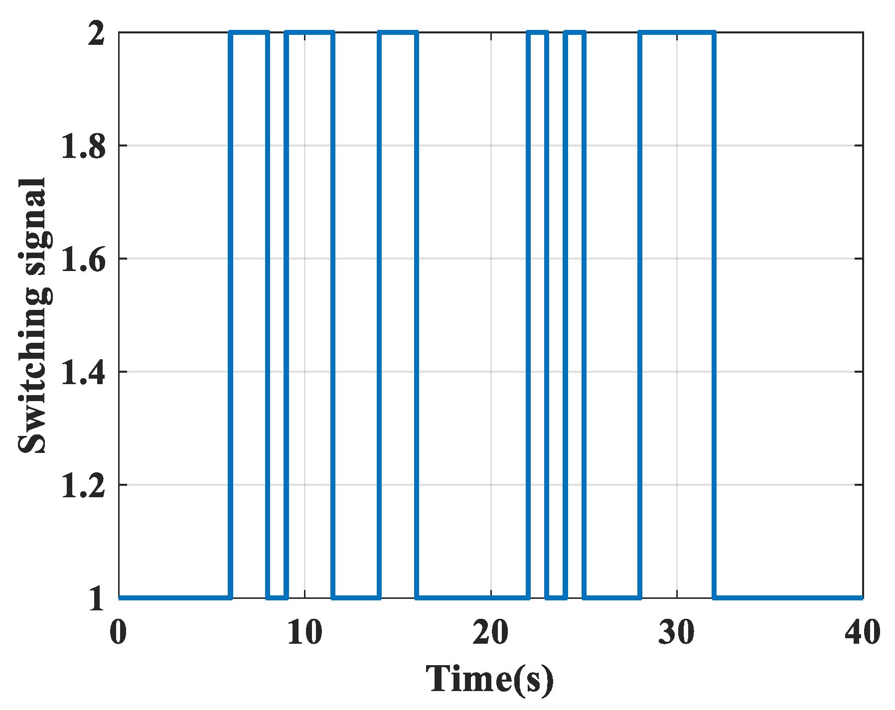
4.1. Design of the PDT Switching Signal

Consider a s = 0.1 , b = 1.08 , L = 10   s , and r = 0.5   Hz . First, the allowable interval of the persistent dwell time ( τ Z ) is calculated. Using (20), it can be found that τ Z = 4.38   s . Therefore, the switching signal’s class is established. Figure 1 indicates a member of the designed class that meets the above-mentioned specifications. In fact, the switching signal shown in Figure 1 can be divided into stages, where each stage confirms τ Z 4.38   s , L p L = 10   s , and r 0.5   Hz . In general, the switching signals that are members of this designed class guarantee the asymptotic stability of the closed-loop system.

4.2. Calculation of the Disturbance Attenuation Level

By selecting γ = 1 , τ Z = 5   s , and using (21), we can find γ J = 1.49 . This value shows the effect level of disturbances on the controlled output despite consecutive switchings. In fact, the switching rate, the decreasing rate of the Lyapunov functional, and the ‘jump high’ coefficient affect the amount of disturbance attenuation.

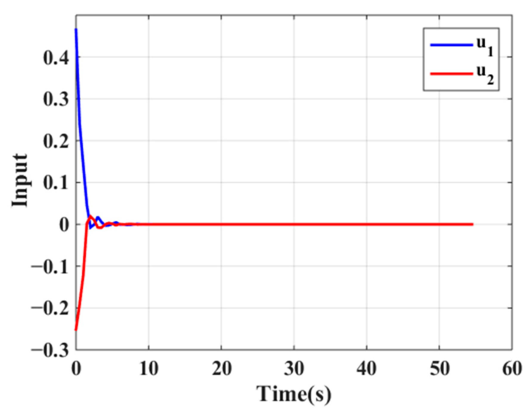
4.3. Simulation of the Model Predictive Controller

Consider n ( k ) = cos ( k ) e 0.4 k , n max = 3 , i e , max = 1   ( e = 1 , 2 , 3 ) , s f , max = 1    ( f = 1 , 2 ) , and s ( 0 ) = ( 0.5     0.8 ) T . By solving the optimization problem in (22)–(27) using the Yalmip toolbox (version R20210331), the following steps are used to obtain the feedback control gain at the beginning:
F 1 , 0 = 0.6979 0.1547 0.1594 0.6497 0 0 .
The variables satisfying the problem in (22)–(27) are obtained in any step in accordance with Figure 1. Based on computer specifications, the maximum time required to solve the problem at every time stage is 0.41 s. Creating a time-variant control gain and reducing the constraints on the controller design based on the proposed framework reduces the design’s conservatism. Figure 2 shows the obtained control input ( i i , k ( k ) = F i , k s ( k ) ). This figure shows that the elements of the control input have lower absolute values than 1, which confirms that the input constraints ( i e , max = 1    ( e = 1 , 2 , 3 ) ) are met. Figure 3 shows the general view of energy variation for the delayed switched system resulting from the multiple Lyapunov functional. Figure 3 shows how the stabilizable sub-systems balance out any potential rise during switching moments caused by the “jump high” condition before the system energy eventually reach zero. Consequently, the system is able to withstand the effects of exogenous disturbances and state delays. Therefore, the proposed scheme guarantees the uniform asymptotic stability of the closed-loop switched system. The existence of the ‘jump high’ condition at the switching instants in the MLKF reduces the conservatism of the controller design compared with the SLKF. In fact, this condition allows the energy to increase at the switching moments and eliminates the condition of strict energy reduction at the switching moments caused by the SLKF. The closed-loop switched system’s state responses as a consequence of the simulation are shown in Figure 4. The simultaneous running of the switching law and the problem in (22)–(27) leads to the system states converging to zero and guaranteeing the H∞ performance. Also, Figure 4 shows that the elements of the states have absolute values of less than 1, which confirms that the state constraints ( x f , max = 1    ( f = 1 , 2 ) ) are satisfied.
Example 2. 
Take into account the discrete-time switched system with three sub-systems [31].
Sub-system 1:
R 1 = 1.4 0.1 0.4 0.2 ,     R m 1 = 0 0.1 0.2 0 ,      S 1 = 2 1 0.6 1 ,       T 1 = 0.1 0.1 T ,     Y 1 = I 2 ,     Z 1 = I 2 ,     m M = 4 ,     L s = 0.5 s ,
where  R 1 R m 1 , S 1 , and T 1 are the state-space matrices for sub-system 1.
Sub-system 2:
R 2 = 1.1 0.2 0.3 0.4 ,     R d 2 = 0 0.1 0.2 0 ,      S 2 = 1 4 3 1 ,       T 2 = 0.1 0.1 T ,     Y 2 = I 2 ,     Z 2 = I 2 ,     m M = 4 ,     L s = 0.5 s ,
where  R 2 , R m 2 , S 2 , and T 2 are the state-space matrices for sub-system 1.
Sub-system 3:
R 3 = 0.8 0.3 0.1 0.2 ,     R d 3 = 0 0.1 0.2 0 ,      S 3 = 3 2 2 0.5 ,       T 3 = 0.1 0.1 T ,     Y 3 = I 2 ,     Z 3 = I 2 ,     m M = 4 ,     L s = 0.5 s ,
where  R 3 , R m 3 , S 3 , and T 3 are the state-space matrices for sub-system 1.
Similar to Example 1, the performance analysis is performed in several sub-sections, which will be discussed in the following.

4.4. Design of the PDT Switching Signal

Consider a s = 0.05 , b = 1.1 , L = 12   s , r = 0.25   Hz , and γ = 1 . Using (20), it can be determined that τ Z = 5.57 . Therefore, the class of switching signals is determined. Figure 5 indicates a member of the designed class that meets the above-mentioned specifications. In fact, the switching signal shown in Figure 5 can be divided into sub-intervals that each sub-interval confirms, such that τ Z 5.57   s , L p L = 12   s , and r 0.25   Hz .

4.5. Calculation of the Disturbance Attenuation Level

By selecting τ Z = 6 s and also using (21), γ J = 1.57 . Equation (21) shows that the ‘jump high’ coefficient and switching rate affect the disturbance attenuation level.

4.6. Simulation of the Model Predictive Controller

Consider n ( k ) = cos ( k ) e 0.3 k    , n max = 3 , i e , max = 1    ( e = 1 , 2 ) , s f , max = 1    ( f = 1 , 2 ) , and s ( 0 ) = ( 0.5     0.6 ) T . The following is how the state feedback control rule at the instant of the beginning is determined:
F 1 , 0 = 0.5219 0.0098 0.2023 0.1382
The variables satisfying the problem in (22)–(27) are obtained in any step in accordance with Figure 6. Based on the computer specifications, the maximum time required to solve the problem at every time stage is 0.39 s. The acquired control input and state responses of the closed-loop switched system are demonstrated in Figure 6 and Figure 7, respectively. It is concluded from Figure 6 and Figure 7 that the input and state constraints are satisfied ( i e , max = 1    ( e = 1 , 2 ) ,     s f , max = 1    ( f = 1 , 2 ) ). Figure 7 shows how the stabilizable sub-systems balance out any potential rise during switching moments caused by the “jump high” condition before the states eventually reach zero. Consequently, the system is able to withstand the effects of exogenous disturbances and state delays. Therefore, the proposed scheme guarantees the H∞ criterium.

5. Conclusions

In this paper, for delayed linear switched systems affected by physical limitations and exogenous disturbances, a concurrent design of the MPC plan and PDT switching signal utilizing the conventional MLKF was established. The conventional MLKF with a ‘jump high’ condition was used as a step forward to reduce the strictness of constraints on the controller design compared with the SLKF. However, the ‘jump high’ condition imposes a dwell-time limitation on the switching signal. Therefore, the PDT structure was used to reduce the dwell-time constraint compared with other structures. Also, a new online framework was proposed to decrease the number of constraints on the controller design at each time step. Moreover, for the first time, the exogenous disturbances were considered in the procedure of MPC design for delayed switched systems, and the non-weighted H∞ performance was guaranteed. The simulation results demonstrate the suggested plan’s great performance and ability to asymptotically stabilize the switched system. Due to the existence of a delay between the switching of sub-systems and the switching of controllers in switched systems, the development of the suggested scheme for the asynchronous switched systems can pose an interesting challenge for future research. Also, the MPC design for the LPV systems to handle the uncertainties of the switching signal can be extended to linear switched systems in a future work.

Author Contributions

Conceptualization, Y.F.H. and M.K.H.Z.; Methodology, Y.F.H. and M.K.H.Z.; Software, Y.F.H.; Validation, Y.F.H.; Formal analysis, M.K.H.Z. and M.J.A.; Investigation, M.J.A., H.D. and H.C.; Resources, H.D.; Writing—original draft, Y.F.H. and M.K.H.Z.; Writing—review & editing, M.J.A., H.D. and H.C.; Project administration, H.C. All authors have read and agreed to the published version of the manuscript.

Funding

This research received no external funding.

Data Availability Statement

The data will be available upon reasonable request.

Conflicts of Interest

The authors declare no conflict of interest.

Appendix A

Proof of Theorem 1. 
The candidate multiple Lyapunov–Krasovskii functional and Lyapunov stability limitation are taken into account:
g σ ( k ) ( k ) = i = 1 2 g σ ( k ) , i ( k ) ,     g σ ( k ) , 1 ( k ) = s T ( k ) C σ ( k ) s ( k ) ,                 g σ ( k ) , 2 ( k ) = i = k m k 1 s T ( i ) C m σ ( k ) s ( i ) ,
g σ ( k + J + 1 | k ) ( k + J + 1 | k ) g σ ( k + J | k ) ( k + J | k ) a s g σ ( k + J | k ) ( k + J | k ) + c T ( k + J | k ) c ( k + J | k ) γ 2 n T ( k + J | k ) n ( k + J | k ) ,
where  g σ ( k ) is the candidate Lyapunov function. This function is considered as the sum of a delay-independent term ( g σ ( k ) , 1 ) and a delay-dependent term ( g σ ( k ) , 2 ( k ) ) to increase the possibility of finding a solution for the optimization problem.
Step 1: In this step, the minimizing problem of the cost function in (9) is formulated as the relations in (13) and (14). The relations in (13) and (14) guarantee the cost function in (9) is minimized and optimal input control is obtained.
By summing both sides of (A2) from 0 to :
J = 0 [ g σ ( k + J + 1 | k ) ( k + J + 1 | k ) g σ ( k + J | k ) ( k + J | k ) ] a s J = 0 v σ ( k + J | k ) ( k + J | k ) J = 0 c ( k + J | k ) T c ( k + J | k ) + γ 2 J = 0 n ( k + J | k ) T n ( k + J | k ) .
By approximating the candidate function at infinity, it equals zero, and we have:
g σ ( k | k ) ( k | k ) γ 2 n max J = 0 c ( k + J | k ) T c ( k + J | k ) J k s T ( k | k ) C σ ( k | k ) s ( k | k ) + i = k m k 1 s T ( i | k ) C m σ ( k | k ) s ( i | k ) + γ 2 n max .
Considering u k as the upper bound of the cost function, we obtain:
s T ( k ) C σ ( k ) s ( k ) + i = k m k 1 s T ( i ) C m σ ( k ) s ( i ) + γ 2 n max u k u k s T ( k ) C σ ( k ) s ( k ) i = k m k 1 s T ( i ) C m σ ( k ) s ( i ) + γ 2 n max 0 .
Due to m m M , if (A6) meets, then (A5) meets:
u k s T ( k ) C σ ( k ) s ( k ) i = k m M k 1 s T ( i ) C m σ ( k ) s ( i ) + γ 2 n max 0 .
Due to Lemma 1, (A6) can be reformulated as:
u k s ( k ) γ 2 n max s ( k 1 ) s ( k m M ) T C σ ( k ) 1 0 0 0 γ 2 n max 0 0 C m σ ( k ) 1 0 C m σ ( k ) 1 1 s ( k ) γ 2 n max s ( k 1 ) s ( k m M ) 0 u k s ( k ) T γ 2 n max s ( k 1 ) T s ( k m M ) T C σ ( k ) 1 0 0 0 γ 2 n max 0 0 C m σ ( k ) 1 0 C m σ ( k ) 1 0 .
Step 2: In this step, the input and state limitations in (5) and (6) are formulated as the relations in (15) and (16). The relations in (15) and (16) guarantee the input control is obtained in such a way that the input and state do not exceed the considered saturation level.
By summing the two sides of (A2) from 0 to l:
J = 0 j [ g σ ( k + J + 1 | k ) ( k + J + 1 | k ) g σ ( k + J | k ) ( k + J | k ) ] a s J = 0 j v σ ( k + J | k ) ( k + J | k ) J = 0 j c ( k + J | k ) T c ( k + J | k ) + γ 2 J = 0 j n ( k + J | k ) T n ( k + J | k ) v σ ( k + j + 1 | k ) ( k + j + 1 | k ) g σ ( k | k ) ( k | k ) a s J = 0 j v σ ( k + J | k ) ( k + J | k ) J = 0 j c ( k + J | k ) T c ( k + J | k ) + γ 2 J = 0 j n ( k + J | k ) T n ( k + J | k ) g σ ( k + j + 1 | k ) ( k + j + 1 | k ) g σ ( k | k ) ( k | k ) + γ 2 n max u k s ( k + j + 1 | k ) T C σ ( k + j + 1 | k ) s ( k + j + 1 | k ) + i = k + j + 1 m k + j s T ( i | k ) C m σ ( k + j + 1 | k ) s ( i | k ) u k s ( k + j + 1 | k ) T C σ ( k + j + 1 | k ) s ( k + j + 1 | k ) u k .
Consider H e and H f as:
H e = ( 0 , ,    1    e t h , , 0 )   ,         H f = ( 0 , ,    1    f t h , , 0 ) .
Using (5), (29), and Lemma 1,
u e ( k + J | k ) 2 = ( F σ ( k + J | k ) s ( k + J | k ) ) e 2 = ( F σ ( k + J | k ) , k C σ ( k + J | k ) 1 2 C σ ( k + J | k ) 1 2 s ( k + J | k ) ) e 2 u k ( F σ ( k + J | k ) C σ ( k + J | k ) 1 2 ) e 2 = u k H e T F σ ( k + J | k ) C σ ( k + J | k ) 1 F σ ( k + J | k ) T H e i e , max 2 i e , max 2 H e F σ ( k + J | k ) u k 1 C σ ( k + J | k ) 0      i e , max 2 H e F σ ( k ) u k 1 C σ ( k ) 0 .
Using (6), (A8), and Lemma 1,
s f ( k + J | k ) 2 = ( C σ ( k + J | k ) 1 2 C σ ( k + J | k ) 1 2 s ( k + J | k ) ) f 2 u k ( C σ ( k + J | k ) 1 2 ) f 2 = u k H e s L C σ ( k + J | k ) 1 H f s e , max 2 s f , max 2 H f u k 1 C σ ( k + J k ) 0 s f , max 2 H f u k 1 C σ ( k ) .
Step 3: In this step, the stability boundary limitation (A12) is formulated as the relation in (17). The relation in (17) guarantees that the energy increase at the switching moments does not exceed a predetermined value.
g σ ( k ) ( s ( k ) ) b   g σ ( k 1 ) ( s ( k ) ) .
Inequality (A12) is extended as follows:
s ( k ) T C σ ( k ) s ( k ) + i = k m k 1 s ( i ) C m σ ( k ) s ( i ) b   g σ ( k 1 ) ( s ( k ) ) b   g σ ( k 1 ) ( s ( k ) ) s ( k ) T C σ ( k ) s ( k ) i = k m k 1 s ( i ) C m σ ( k ) s ( i ) 0 .
Due to m m M , if (A14) meets, then (A13) meets:
b   g σ ( k 1 ) ( s ( k ) ) s T ( k ) C σ ( k ) s ( k ) i = k m M k 1 s ( i ) C m σ ( k ) s ( i ) 0 .
Using Lemma 1,
b   g σ ( k 1 ) ( s ( k ) ) i = k m M k 1 s ( i ) C m σ ( k ) s ( i ) s T ( k ) C σ ( k ) 1 0 b g σ ( k 1 ) ( s ( k ) ) s ( k 1 ) T s ( k m M ) T s T ( k ) C m σ ( k ) 1 0 0 C m σ ( k ) 1 0 C σ ( k ) 1 0 .
Step 4: In this step, the Lyapunov stability limitation (A2) is formulated as the relation in (18). The relation in (18) is a necessary limitation to satisfy the H∞ performance.
Δ g 1 is expanded as follows:
Δ g 1 = ( R ¯ σ ( k + J | k ) s ( k + J | k ) + R m σ ( k + J | k ) s ( k + J m | k ) + T σ ( k + J | k ) n ( k + J | k ) ) T C σ ( k + J + 1 | k ) ( R ¯ σ ( k + J | k ) s ( k + J | k ) + R m σ ( k + J | k ) s ( k + J m | k ) + T σ ( k + J | k ) n ( k + J | k ) ) s T ( k + J | k ) C σ ( k + J | k ) s ( k + J | k ) .
Using Lemma 1,
Δ g 1 s T ( k ) R ¯ σ ( k ) T C σ ( k ) R ¯ σ ( k ) s ( k ) + s T ( k ) R ¯ σ ( k ) T C σ ( k ) R m σ ( k ) s ( k m ) + s T ( k ) R ¯ σ ( k ) T C σ ( k ) T σ ( k ) n ( k ) + s T ( k m ) R m σ ( k ) T C σ ( k ) R ¯ σ ( k ) s ( k ) + s T ( k m ) R m σ ( k ) T C σ ( k ) R m σ ( k ) s ( k m ) + s T ( k m ) R m σ ( k ) T C σ ( k ) T σ ( k ) n ( k ) + n ( k ) T T σ ( k ) T C σ ( k ) R ¯ σ ( k ) s ( k ) + n ( k ) T T σ ( k ) T C σ ( k ) R m σ ( k ) s ( k m ) + n ( k ) T T σ ( k ) T C σ ( k ) T σ ( k ) n ( k ) s T ( k ) C σ ( k ) s ( k ) .
By extending Δ v 2 ,
Δ g 2 = s ( k ) T C m σ ( k ) s ( k ) s ( k m ) T C m σ ( k ) s ( k m ) .
Substituting (A17) and (A18) into (A2),
s T ( k ) R ¯ σ ( k ) T C σ ( k ) R ¯ σ ( k ) x ( k ) + s T ( k ) R ¯ σ ( k ) T C σ ( k ) R m σ ( k ) s ( k m ) + s T ( k ) R ¯ σ ( k ) T C σ ( k ) T σ ( k ) n ( k ) + s T ( k m ) R m σ ( k ) T C σ ( k ) R ¯ σ ( k ) s ( k ) + s T ( k m ) R m σ ( k ) T C σ ( k ) R m σ ( k ) s ( k m ) + s T ( k m ) R m σ ( k ) T C σ ( k ) T σ ( k ) n ( k ) + n ( k ) T T σ ( k ) T C σ ( k ) R ¯ σ ( k ) s ( k ) + n ( k ) T T σ ( k ) T C σ ( k ) R m σ ( k ) s ( k m ) + n ( k ) T T σ ( k ) T C σ ( k ) T σ ( k ) n ( k ) s T ( k ) C σ ( k ) s ( k ) + s ( k ) T C m σ ( k ) s ( k ) s ( k m ) T C m σ ( k ) s ( k m ) + s T ( k ) Y σ ( k ) T Y σ ( k ) s ( k ) + s T ( k ) F σ ( k ) T Z σ ( k ) T Z σ ( k ) F σ ( k ) s ( k ) γ 2 n T ( k ) n ( k ) a s s ( k ) T C σ ( k ) s ( k ) a s i = k m k 1 s ( i ) C m σ ( k ) s ( i ) 0 .
Due to m m M , if (A20) meets, then (A19) meets:
s T ( k ) R ¯ σ ( k ) T C σ ( k ) A ¯ σ ( k ) s ( k ) + s T ( k ) R ¯ σ ( k ) T C σ ( k ) R d σ ( k ) s ( k m ) + s T ( k ) R ¯ σ ( k ) T C σ ( k ) T σ ( k ) n ( k ) + s T ( k m ) R m σ ( k ) T C σ ( k ) R ¯ σ ( k ) s ( k ) + s T ( k m ) R m σ ( k ) T C σ ( k ) R m σ ( k ) s ( k m ) + s T ( k m ) R m σ ( k ) T C σ ( k ) T σ ( k ) s ( k ) + s ( k ) T T σ ( k ) T C σ ( k ) R ¯ σ ( k ) s ( k ) + x ( k ) T T σ ( k ) T C σ ( k ) R m σ ( k ) s ( k d ) + s ( k ) T T σ ( k ) T C σ ( k ) T σ ( k ) n ( k ) s T ( k ) C σ ( k ) s ( k ) + s ( k ) T C m σ ( k ) s ( k ) s ( k m ) T C m σ ( k ) s ( k m ) + s T ( k ) Y σ ( k ) T Y σ ( k ) s ( k ) + s T ( k ) F σ ( k ) T Z σ ( k ) T Z σ ( k ) F σ ( k ) s ( k ) γ 2 n T ( k ) n ( k ) a s ( k ) T C σ ( k ) s ( k ) a s i = k m M k 1 s ( i ) C m σ ( k ) s ( i ) 0 .
Inequality (A20) can be formulated as:
s ( k ) s ( k m ) n ( k ) s ( k 1 ) s ( k m M ) T L 11 L 12 L 13 0 L 22 L 23 0 L 33 0 a s C m σ ( k )              0 0 0 0 a s C m σ ( k )   s ( k ) s ( k m ) n ( k ) s ( k 1 ) s ( k m M ) 0 .
Inequality (A22) holds if (A21) is met:
L 11 L 12 L 13 0 L 22 L 23 0 L 33 0 a s C m σ ( k )              0 0 0 0 a s C m σ ( k ) 0 .
Step 5: In this step, the PDT switching signal is designed to satisfy the H∞ performance.
To design the switching signal, it is necessary to have the stability condition at the actual time steps. Inequality (A2), which confirms the stability condition at the prediction horizon, does not guarantee the stability condition at the actual time steps. In this regard, it is important to realize this guarantee in the form of the optimization problem described in (13)–(18). Therefore, Lemma 2 is introduced as follows.
Lemma A1. 
The optimization problem in (13)(18) guarantees the stability condition at the actual time steps as follows:
g σ ( k + 1 ) ( k + 1 ) ( 1 + a s ) g σ ( k ) ( k ) c ( k ) T c ( k ) + γ 2 n ( k ) T n ( k ) .
Proof of Lemma A1. 
According to (A5) and (A8),
g σ ( k + 1 | k ) ( k + 1 | k ) = s ( k + 1 | k ) T C σ ( k + 1 | k ) s ( k + 1 | k ) u k ,
g σ ( k + 1 | k + 1 ) ( k + 1 | k + 1 ) = s ( k + 1 | k + 1 ) T C σ ( k + 1 | k + 1 ) s ( k + 1 | k + 1 ) u k + 1 γ 2 n max .
Based on (A24) and (A25), it is inferred that if  ( u k , C σ ( k + 1 | k ) )  is a feasible answer at step k + 1, then:
g σ ( k + 1 | k ) ( k + 1 | k ) = s ( k + 1 | k ) T C σ ( k + 1 | k ) s ( k + 1 | k ) u k γ 2 n max .
Therefore,  ( u k , C σ ( k + 1 | k ) ) is a feasible answer, and ( u k + 1 , C σ ( k + 1 | k + 1 ) )  is an optimal answer at step k + 1 ( u k + 1 u k ). Therefore,
g σ ( k + 1 | k + 1 ) ( k + 1 | k + 1 ) g σ ( k + 1 | k ) ( k + 1 | k ) ( 1 + a s ) g σ ( k | k ) ( k | k ) c ( k | k ) T c ( k | k ) + γ 2 n ( k | k ) T n ( k | k ) g σ ( k + 1 ) ( k + 1 ) ( 1 + a s ) g σ ( k ) ( k ) c ( k ) T c ( k ) + γ 2 n ( k ) T n ( k ) .
Now, if  ( u k , C σ ( k + 1 | k ) )  is not a feasible answer at step k + 1, then:
g σ ( k ) ( k + 1 | k ) = s ( k + 1 | k ) T C σ ( k + 1 | k ) s ( k + 1 | k ) u k γ 2 n max     ( u k < u k ) .
Therefore,  ( u k , C σ ( k + 1 | k ) ) is a feasible answer, and ( u k + 1 , C ( k + 1 | k + 1 ) )  is an optimal answer at step k + 1 ( u k + 1 u k ). In this regard, (A27) is also obtained. □
Remark A1. 
Lemma A1 only demonstrates that stability conditions over the predictive time steps guarantee stability conditions at the actual time steps. Now, using the stability conditions at the actual time steps, the switching signal is designed, and the disturbance attenuation level is achieved. The designed switching signal, along with the constraints derived in steps 1 to 4 of proof of Theorem 1, satisfies the H∞ performance and the system constraints.
Based on (A12) and (A27), the PDT switching rule is designed in such a way that the H∞ criterium is held for the system in (1)–(3). Therefore, Definition 1 must be held as follows:
(1)
Proof of asymptotical stability with  s ( k 0 ) 0 and n ( k ) = 0
Assume σ ( k s p + 1 ) = n , and   σ ( k s p ) = m . Due to Definition 2, (A12), and (A27), the Lyapunov function varies as follows in the eth sub-interval’s total time duration:
g n ( s ( k s p + 1 ) ) b ( 1 + a s ) g σ ( k s p + 1 1 ) ( s ( k s p + 1 1 ) ) b ( 1 + a s ) k s p + 1 k s p + 1 1 g σ ( k s p + 1 1 ) ( s ( k s p + 1 1 ) ) b I ( k s p + 1 , k s p + 1 ) ( 1 + a s ) k s p + 1 k s p + 1 g σ ( k s p + 1 ) ( s ( k s p + 1 ) ) b I ( k s p , k s p + 1 ) + 1 ( 1 + a s ) k s p + 1 k s p g σ ( k s p ) ( s ( k s p ) ) b L r + 1 ( 1 + a s ) τ Z g m ( s ( k s p ) ) .
These changes should decrease. The following inequality must be satisfied as a result:
κ = b L r + 1 ( 1 + a s ) τ Z < 1 e ( L r + 1 ) ln b + τ ln ( 1 + a s ) < 1 ( L r + 1 ) ln b + τ Z ln ( 1 + a s ) < 0 τ Z > τ Z = ( L r + 1 ) ln b ln ( 1 + a s ) .
The Lyapunov function’s change if there are e sub-intervals throughout the specified time interval is:
g n ( s ( k s p + 1 ) ) κ p   g σ ( k s 1 ) ( s ( k s 1 ) ) .
Considering k s 1 = k 0 , k [ k s p + 1 , k s p + 2 ) , and (A12) and (A27),
g σ ( k ) ( s ( k ) ) b L r + 1   κ p   g σ ( k 0 ) ( s ( k 0 ) ) s ( k ) κ 1 1 ( b L r + 1   κ p κ 2 ( s ( k 0 ) ) ) s ( k ) κ 3 ( s ( k 0 ) ) ) ,
where
κ 1 = λ min ( C σ ( k ) ) s ( k ) 2   ,     κ 2 = λ max ( C σ ( k 0 ) ) s ( k 0 ) 2 .
Therefore, (A30) guarantees (A32) and also k s ( k ) 0 . Therefore, the closed-loop system is asymptotically stable.
(2)
Proof of  k = 0 c T ( k ) c ( k ) γ 2 k = 0 n T ( k ) n ( k ) with s ( k 0 ) = 0 and n ( k ) 0
Consider Γ ( k ) = c ( k ) T c ( k ) γ 2 n ( k ) T n ( k ) . Due to Definition 2, (A12), and (A27), the Lyapunov function varies as follows in the eth sub-interval’s total time duration:
g n ( s ( k s p + 1 ) ) b ( 1 + a s ) g σ ( k s p + 1 1 ) ( s ( k s p + 1 1 ) ) b Γ ( k s p + 1 1 ) b I ( k s p + 1 , k s p + 1 ) + 1 ( 1 + a s ) k s p + 1 k s p g m ( s ( k s p ) ) b Γ ( k s p + 1 1 ) b ( 1 + a s ) Γ ( k s p + 1 2 ) b ( 1 + a s ) k s p + 1 k s p + 1 1 Γ ( k s p + 1 1 ) b I ( k s p + 1 , k s p + 1 ) ( 1 + a s ) k s p + 1 k s p + 1 Γ ( k s p + 1 ) b I ( k s p , k s p + 1 ) ( 1 + a s ) k s p + 1 k s p Γ ( k s p ) κ p   g σ ( k s 1 ) ( s ( k s 1 ) ) J = k s 1 k s p + 1 b I ( J , k s p + 1 ) ( 1 + a s ) k s p + 1 J Γ ( J ) .
Assuming k s 1 = k 0 , k [ k s p + 1 , k s p + 2 ) , and (A12) and (A27),
g σ ( k ) ( s ( k ) ) b L r + 1   κ p   g σ ( k 0 ) ( s ( k 0 ) ) J = k 0 k b I ( J , k ) ( 1 + a s ) k L Γ ( J ) .
Selecting the zero initial conditions and due to g σ ( k ) ( s ( k ) ) 0 , we have:
J = k 0 k b I ( J , k ) ( 1 + a s ) k J Γ ( J ) 0 .
Let us extend (A36) as follows:
J = k 0 k [ b I ( J , k ) ( 1 + a s ) k J c ( J ) T c ( J ) ] γ 2 J = k 0 k [ b I ( J , k ) ( 1 + a s ) k J n ( J ) T n ( J ) ] J = k 0 k ( 1 + a s ) k J c ( J ) T c ( J ) γ 2 J = k 0 k b I ( J , k ) ( 1 + a s ) k J n ( J ) T n ( J ) .
τ p + L p is the total execution duration in the eth sub-interval, and τ p and L p are the execution duration in the τ-part and the L -part, respectively. Since L p L , and τ p τ Z , and supposing τ Z r > 1 , it is concluded that ( τ Z r 1 ) ( L p L ) 0 . Therefore, for the time interval [ J , k ] , we have:
I ( J , k ) ( k J J p + τ p + 1 ) ( J p r + 1 ) ( k J J + τ Z + 1 ) ( J r + 1 ) .
Substituting (A38) into (A37), results in:
J = k 0 k ( 1 + a s ) k J c ( J ) T c ( J ) γ 2 J = k 0 k b ( k J L + τ Z + 1 ) ( L r + 1 ) ( 1 + a s ) k J n ( J ) T n ( J ) J = k 0 k ( 1 + a s ) k J c ( J ) T c ( J ) γ 2 b L r + 1 J = k 0 k [ b ( k J L + τ Z ) ( L r + 1 ) ( 1 + a s ) k J n ( J ) T n ( J ) ] k = k 0 J = k 0 k ( 1 + a s ) k J c ( J ) T c ( J ) γ 2 b L r + 1 k = k 0 J = k 0 k ( b L r + 1 L + τ Z ) k J   ( 1 + a s ) k J n ( J ) T n ( J ) J = k 0 k = J ( 1 + a s ) k J c ( J ) T c ( J ) γ 2 b L r + 1 J = k 0 J = k 0 k ( b L r + 1 L + τ Z ) k J   ( 1 + a s ) k J n ( J ) T n ( J ) .
Due to 0 < 1 + a s < 1 and 0 < b L r + 1 L + τ Z ( 1 + a s ) < 1 , (A39) can be rewritten as follows:
J = k 0 1 a s c ( J ) T c ( J ) γ 2 b L r + 1 J = k 0 1 1 b L r + 1 L + τ Z ( 1 + a s ) n ( J ) T n ( J ) J = k 0 c ( J ) T c ( J ) a s γ 2 b L r + 1 1 b L r + 1 L + τ Z ( 1 + a s ) J = k 0 n ( J ) T n ( J ) .
Therefore, (21) is validated and Theorem 1 is proved. □

Appendix B

Proof of Theorem 2. 
Consider  v σ ( k ) = u k   C σ ( k ) 1 , t σ ( k ) = u k   C m σ ( k ) 1 , o σ ( k ) = u k   N σ ( k ) , and q σ ( k ) = F σ ( k )   o σ ( k ) . Firstly, the LMI limitation related to (14) is proved. Also, (23) is calculated by multiplying (A6) by u k 1 and applying Lemma 1. Second, the LMI limitations related to the input and states constraints in (15)–(16) are obtained:
i e i , max 2 H e i F σ ( k ) u k 1 C σ ( k ) 0 i e i , max 2 H e i F σ ( k ) v σ ( k ) 1 0 I 0 0 o σ ( k ) T v e v , max 2 H e i F σ ( k ) v σ ( k ) 1 I 0 0 o σ ( k ) 0 i e i , max 2 H e i F σ ( k ) o σ ( k ) o σ ( k ) T v σ ( k ) 1 o σ ( k ) 0 i e i , max 2 H e i q σ ( k ) o σ ( k ) T v σ ( k ) 1 o σ ( k ) 0 ,
s e s , max 2 H e s u k 1 C σ ( k ) 0 o e o , max 2 H e o v σ ( k ) 1 0 I 0 0 o σ ( k ) T o e s , max 2 H e s v σ ( k ) 1 I 0 0 o σ ( k ) 0 o e s , max 2 H e s o σ ( k ) o σ ( k ) T v σ ( k ) 1 o σ ( k ) 0 .
From the feasibility of (A41) and (A42), it can be concluded that  o σ ( k ) T v σ ( k ) 1 o σ ( k ) > 0 . Therefore, o σ ( k ) is full-rank. Developing ( v σ ( k ) o σ ( k ) ) T v σ ( k ) 1 ( v σ ( k ) o σ ( k ) ) 0 ,
o σ ( k ) T v σ ( k ) 1 o σ ( k ) o σ ( k ) + o σ ( k ) T v σ ( k ) .
According to (A43), if inequalities (24) and (25) hold, then inequalities (A41) and (A42) are also held. Thirdly, the LMI limitation related to the boundary limitation of Lyapunov stability in (17) is proved. Multiplying (A12) by  u k  and utilizing Lemma 1, inequality (26) is obtained. Eventually, the LMI limitation related to the Lyapunov stability limitation of the sub-systems in (18) is proved. As such, (18) can be reformulated:
L 11 0 0 0 L 22 0 0 L 33 0 a s C m σ ( k )        0 0 0       0 0 0 0 a s C m σ ( k ) R ¯ σ ( k ) T R m σ ( k ) T T σ ( k ) T 0 0 C σ ( k ) R ¯ σ ( k ) R d σ ( k ) T σ ( k ) 0 0 0 .
Based on Lemma 1 and (A44), we obtain:
L 11 0 0 0 0 0 R ¯ σ ( k ) T L 22 0 0 0 0 R m σ ( k ) T L 33 0 0 0 T σ ( k ) T a s C m σ ( k ) 0 0 a s C m σ ( k ) 0 C σ ( k ) 1 0 .
Considering  C σ ( k ) = E σ ( k ) 1 and   C m σ ( k ) = D σ ( k ) 1 , we have:
( 1 + a s ) E σ ( k ) 1 D σ ( k ) 1 Y σ ( k ) T Y σ ( k ) F σ ( k ) T Z σ ( k ) T Z σ ( k ) F σ ( k ) 0 0 0 0 0 R ¯ σ ( k ) T D σ ( k ) 1 0 0 0 0 R m σ ( k ) T γ 2 I 0 0 0 T σ ( k ) T a s D σ ( k ) 1 0 0 a s D σ ( k ) 1 0 E σ ( k ) 0 .
By multiplying the left and right sides (A46) by  b d i a g ( N σ ( k ) T , N σ ( k ) T , I , N σ ( k ) T , , N σ ( k ) T , I ) and b d i a g ( N σ ( k ) , N σ ( k ) , I , N σ ( k ) , , N σ ( k ) , I ) , respectively,
b Λ σ ( k ) 1 α 1 σ ( k ) 2 N σ ( k ) T F σ ( k ) T F σ ( k ) N σ ( k ) ( 1 + a s ) N σ ( k ) T E σ ( k ) 1 N σ ( k ) N σ ( k ) T D σ ( k ) 1 N σ ( k ) N σ ( k ) T Y σ ( k ) T Y σ ( k ) N σ ( k ) N σ ( k ) T F σ ( k ) T Z σ ( k ) T Z σ ( k ) F σ ( k ) N σ ( k ) 0 0 0 0 0 N σ ( k ) T R ¯ σ ( k ) T D σ ( k ) 1 0 0 0 0 R d σ ( k ) T γ 2 I 0 0 0 T σ ( k ) T a s N σ ( k ) T D σ ( k ) 1 N σ ( k ) 0 0 a s N σ ( k ) T D σ ( k ) 1 N σ ( k ) 0 E σ ( k ) 0 .
Multiplying (A47) by  u k and using Lemma 1 many times and using the mentioned variables above,
( 1 + a s ) o σ ( k ) T v σ ( k ) 1 o σ ( k ) o σ ( k ) T o σ ( k ) T Y σ ( k ) T q σ ( k ) T Z σ ( k ) T 0 0 t σ ( k ) 0 0 0 0 u k I 0 0 0 u k I 0 0 o σ ( k ) T t σ ( k ) 1 o σ ( k ) 0 u k γ 2 I 0 0 o σ ( k ) T R σ ( k ) T + q σ ( k ) T S σ ( k ) T 0 0 0 0 0 0 0 0 0 0 0 R m σ ( k ) T 0 0 u k T σ ( k ) T a s o σ ( k ) T t σ ( k ) 1 o σ ( k ) 0 0 a o o σ ( k ) T t σ ( k ) 1 o σ ( k ) 0 v σ ( k ) 0 .
Based on (A43), it can be said that if (27) meets, (A48) also meets, and Theorem 2 is proven. □

References

  1. Wang, H.; Wu, X.; Zheng, X.; Yuan, X. Model Predictive Current Control of Nine-Phase Open-End Winding PMSMs with an Online Virtual Vector Synthesis Strategy. IEEE Trans. Ind. Electron. 2022, 7, 2199–2208. [Google Scholar] [CrossRef]
  2. Liu, S.; Liu, C. Virtual-Vector-Based Robust Predictive Current Control for Dual Three-Phase PMSM. IEEE Trans. Ind. Electron. 2021, 68, 2048–2058. [Google Scholar] [CrossRef]
  3. Yang, H.; Jiang, B.; Cocquempot, V. A survey of results and perspectives on stabilization of switched nonlinear systems with unstable modes. Nonlinear Anal. Hybrid Syst. 2014, 13, 45–60. [Google Scholar] [CrossRef]
  4. Kai, Y.; Ji, J.; Yin, Z. Study of the generalization of regularized long-wave equation. Nonlinear Dyn. 2022, 107, 2745–2752. [Google Scholar] [CrossRef]
  5. Lin, H.; Antsaklis, P.J. Stability and stabilizability of switched linear systems: A survey of recent results. IEEE Trans. Autom. Control 2009, 54, 308–322. [Google Scholar] [CrossRef]
  6. Mhaskar, P.; El-Farra, N.H.; Christofides, P.D. Robust predictive control of switched systems: Satisfying uncertain schedules subject to state and control constraints. Int. J. Adapt. Control Signal Process. 2008, 22, 161–179. [Google Scholar] [CrossRef]
  7. Ban, J.; Kwon, W.; Won, S.; Kim, S. Robust H∞ finite-time control for discrete-time polytopic uncertain switched linear systems. Nonlinear Anal. Hybrid Syst. 2018, 29, 348–362. [Google Scholar] [CrossRef]
  8. Zhang, H.; Xie, D.; Zhang, D.; Wang, G. Stability analysis for discrete-time switched systems with unstable sub-systems by a mode-dependent average dwell-time approach. ISA Trans. 2014, 53, 1081–1086. [Google Scholar] [CrossRef]
  9. Mhaskar, P.; El-Farra, N.H.; Christofides, P.D. Predictive control of switched nonlinear systems with scheduled mode transitions. IEEE Trans. Autom. Control 2005, 50, 1670–1680. [Google Scholar] [CrossRef]
  10. Bagherzadeh, M.; Ghaisari, J.; Askari, J. Robust exponential stability and stabilisation of parametric uncertain switched linear systems under arbitrary switching. IET Control Theory Appl. 2016, 10, 381–390. [Google Scholar] [CrossRef]
  11. Ding, D.W.; Yang, G.H. Static output feedback for discrete-time switched linear systems under arbitrary switching. Int. J. Control Autom. Syst. 2010, 8, 220–227. [Google Scholar] [CrossRef]
  12. Shi, S.; Fei, Z.; Li, J. Finite-time H∞ control of switched systems with mode-dependent average dwell-time. J. Frankl. Inst. 2016, 353, 221–234. [Google Scholar] [CrossRef]
  13. Ebadollahi, S.; Saki, S. Wind turbine torque oscillation reduction using soft switching multiple model predictive control based on the gap metric and Kalman filter estimator. IEEE Trans. Ind. Electron. 2017, 65, 3890–3898. [Google Scholar] [CrossRef]
  14. Kersting, S.; Buss, M. Direct and indirect model reference adaptive control for multivariable piecewise affine systems. IEEE Trans. Autom. Control 2017, 62, 5634–5649. [Google Scholar] [CrossRef]
  15. Zhao, X.; Yin, Y.; Yang, H.; Li, R. Adaptive control for a class of switched linear systems using state-dependent switching. Circuits Syst. Signal Process. 2015, 34, 3681–3695. [Google Scholar] [CrossRef]
  16. Liu, T.; Wang, C. Quasi-time-dependent asynchronous H∞ control of discrete-time switched systems with mode-dependent persistent dwell-time. Eur. J. Control 2019, 48, 66–73. [Google Scholar] [CrossRef]
  17. Shi, S.; Shi, Z.; Fei, Z. Asynchronous control for switched systems by using persistent dwell-time modeling. Syst. Control Lett. 2019, 133, 104523. [Google Scholar] [CrossRef]
  18. Fan, Y.; Wang, M.; Sun, G.; Yi, W.; Liu, G. Quasi-time-dependent robust H∞ static output feedback control for uncertain discrete-time switched systems with mode-dependent persistent dwell-time. J. Frankl. Inst. 2020, 357, 10329–10352. [Google Scholar] [CrossRef]
  19. Notash, F.Y.; Rodriguez, J.; Tohidi, S. One beat delay predictive current control of a reduced-switch 3-Level VSI-fed IPMSM with minimized torque ripple. In Proceedings of the 2021 IEEE International Conference on Predictive Control of Electrical Drives and Power Electronics (PRECEDE), Jinan, China, 20–22 November 2021; pp. 519–523. [Google Scholar]
  20. Alanazi, M.; Salem, M.; Sabzalian, M.H.; Prabaharan, N.; Ueda, S.; Senjyu, T. Designing a new controller in the operation of the hybrid PV-BESS system to improve the transient stability. IEEE Access 2023, 11, 97625–97640. [Google Scholar] [CrossRef]
  21. Chen, B.; Hu, J.; Zhao, Y.; Ghosh, B.K. Finite-Time Velocity-Free Rendezvous Control of Multiple AUV Systems with Intermittent Communication. IEEE Trans. Syst. Man Cybern. Syst. 2022, 52, 6618–6629. [Google Scholar] [CrossRef]
  22. Ladel, A.A.; Benzaouia, A.; Outbib, R.; Ouladsine, M. Robust fault tolerant control of continuous-time switched systems: An LMI approach. Nonlinear Anal. Hybrid Syst. 2021, 39, 100950. [Google Scholar] [CrossRef]
  23. Hou, Y.; Tong, S. Adaptive fuzzy output-feedback control for a class of nonlinear switched systems with unmodeled dynamics. Neurocomputing 2015, 168, 200–209. [Google Scholar] [CrossRef]
  24. Ma, K.; Li, Z.; Liu, P.; Yang, J.; Geng, Y.; Yang, B.; Guan, X. Reliability-Constrained Throughput Optimization of Industrial Wireless Sensor Networks with Energy Harvesting Relay. IEEE Internet Things J. 2021, 8, 13343–13354. [Google Scholar] [CrossRef]
  25. Yang, X.; Wang, X.; Wang, S.; Wang, K.; Sial, M.B. Finite-time adaptive dynamic surface synchronization control for dual-motor servo systems with backlash and time-varying uncertainties. ISA Trans. 2023, 137, 248–262. [Google Scholar] [CrossRef]
  26. Morsali, P.; Dey, S.; Mallik, A.; Akturk, A. Switching modulation optimization for efficiency maximization in a single-stage series resonant DAB-based DC-AC converter. IEEE J. Emerg. Sel. Top. Power Electron. 2023, 11, 5454–5469. [Google Scholar] [CrossRef]
  27. Wang, Y.; Xu, N.; Liu, Y.; Zhao, X. Adaptive fault-tolerant control for switched nonlinear systems based on command filter technique. Appl. Math. Comput. 2021, 392, 125725. [Google Scholar] [CrossRef]
  28. Benallouch, M.; Schutz, G.; Fiorelli, D.; Boutayeb, M. H∞ model predictive control for discrete-time switched linear systems with application to drinking water supply network. J. Process Control 2014, 24, 924–938. [Google Scholar] [CrossRef]
  29. Li, Q.; Lin, H.; Tan, X.; Du, S. H∞ Consensus for Multiagent-Based Supply Chain Systems Under Switching Topology and Uncertain Demands. IEEE Trans. Syst. Man Cybern. Syst. 2020, 50, 4905–4918. [Google Scholar] [CrossRef]
  30. Yang, X.; Wang, X.; Wang, S.; Puig, V. Switching-based adaptive fault-tolerant control for uncertain nonlinear systems against actuator and sensor faults. J. Frankl. Inst. 2023, 360, 11462–11488. [Google Scholar] [CrossRef]
  31. Yuan, C.; Gu, Y.; Zeng, W.; Stegagno, P. Switching Model Predictive Control of Switched Linear Systems with Average Dwell-time. In Proceedings of the 2020 American Control Conference, Denver, CO, USA, 1–3 July 2020; pp. 2888–2893. [Google Scholar]
  32. Aminsafaee, M.; Shafiei, M.H. Stabilization of uncertain nonlinear discrete-time switched systems with state delays: A constrained robust model predictive control approach. J. Vib. Control 2019, 25, 2079–2090. [Google Scholar] [CrossRef]
  33. Li, S.; Chen, H.; Chen, Y.; Xiong, Y.; Song, Z. Hybrid Method with Parallel-Factor Theory, a Support Vector Machine, and Particle Filter Optimization for Intelligent Machinery Failure Identification. Machines 2023, 11, 837. [Google Scholar] [CrossRef]
  34. Zhang, M.; Yang, X.; Qi, Q.; Park, J.H. State Estimation of Switched Time-Delay Complex Networks with Strict Decreasing LKF. IEEE Trans. Neural Netw. Learn. Syst. 2023. early access. [Google Scholar]
  35. Li, L.; Yao, L. Fault Tolerant Control of Fuzzy Stochastic Distribution Systems with Packet Dropout and Time Delay. IEEE Trans. Autom. Sci. Eng. 2023. early access. [Google Scholar] [CrossRef]
  36. Dai, W.; Zhou, X.; Li, D.; Zhu, S.; Wang, X. Hybrid Parallel Stochastic Configuration Networks for Industrial Data Analytics. IEEE Trans. Ind. Inform. 2022, 18, 2331–2341. [Google Scholar] [CrossRef]
  37. Qi, Y.; Yu, W.; Huang, J.; Yu, Y. Model predictive control for switched systems with a novel mixed time/event-triggering mechanism. Nonlinear Anal. Hybrid Syst. 2021, 42, 101081. [Google Scholar] [CrossRef]
  38. Han, T.; Ge, S.; Li, T. Persistent dwell-time switched nonlinear systems: Variation paradigm and gauge design. IEEE Trans. Automat. Control 2010, 55, 321–337. [Google Scholar]
  39. Bao, Y.; Mohammadpour Velni, J.; Shahbakhti, M. An online transfer learning approach for identification and predictive control design with application to RCCI engines. In Proceedings of the Dynamic Systems and Control Conference, Pittsburgh, PA, USA, 4–7 October 2020; American Society of Mechanical Engineers: New York, NY, USA, 2020; Volume 84270, p. V001T21A003. [Google Scholar]
  40. Bao, Y.; Abbas, H.S.; Mohammadpour Velni, J. A learning-and scenario-based MPC design for nonlinear systems in LPV framework with safety and stability guarantees. Int. J. Control. 2023, 1–20. [Google Scholar] [CrossRef]
  41. Hu, J.; Wu, Y.; Li, T.; Ghosh, B.K. Consensus Control of General Linear Multiagent Systems with Antagonistic Interactions and Communication Noises. IEEE Trans. Autom. Control 2019, 64, 2122–2127. [Google Scholar] [CrossRef]
  42. Yang, X.; Feng, G.; He, C.; Cao, J. Event-Triggered Dynamic Output Quantization Control of Switched T–S Fuzzy Systems with Unstable Modes. IEEE Trans. Fuzzy Syst. 2022, 30, 4201–4210. [Google Scholar] [CrossRef]
Figure 1. Switching signal.
Mathematics 12 00246 g001
Figure 2. The input of the drinking water supply network.
Mathematics 12 00246 g002
Figure 3. The variation in the Lyapunov function in the drinking water supply network.
Mathematics 12 00246 g003
Figure 4. The states of the drinking water supply network.
Mathematics 12 00246 g004
Figure 5. Switching signal.
Mathematics 12 00246 g005
Figure 6. The control input.
Mathematics 12 00246 g006
Figure 7. The system states.
Mathematics 12 00246 g007
Disclaimer/Publisher’s Note: The statements, opinions and data contained in all publications are solely those of the individual author(s) and contributor(s) and not of MDPI and/or the editor(s). MDPI and/or the editor(s) disclaim responsibility for any injury to people or property resulting from any ideas, methods, instructions or products referred to in the content.

