
ANOVA-GP Modeling for High-Dimensional Bayesian Inverse Problems

1
School of Information Science and Technology, ShanghaiTech University, Shanghai 201210, China
2
School of Statistics and Mathematics, Shanghai Lixin University of Accounting and Finance, Shanghai 201209, China
*
Author to whom correspondence should be addressed.
†
These authors contributed equally to this work.
Mathematics 2024, 12(2), 301; https://0-doi-org.brum.beds.ac.uk/10.3390/math12020301
Submission received: 17 December 2023
/
Revised: 10 January 2024
/
Accepted: 14 January 2024
/
Published: 17 January 2024
(This article belongs to the Special Issue Advances in Numerical Linear Algebra and Its Applications)
Abstract
:Markov chain Monte Carlo (MCMC) stands out as an effective method for tackling Bayesian inverse problems. However, when dealing with computationally expensive forward models and high-dimensional parameter spaces, the challenge of repeated sampling becomes pronounced. A common strategy to address this challenge is to construct an inexpensive surrogate of the forward model, which cuts the computational cost of individual samples. While the Gaussian process (GP) is widely used as a surrogate modeling strategy, its applicability can be limited when dealing with high-dimensional input or output spaces. This paper presents a novel approach that combines the analysis of variance (ANOVA) decomposition method with Gaussian process regression to handle high-dimensional Bayesian inverse problems. Initially, the ANOVA method is employed to reduce the dimension of the parameter space, which decomposes the original high-dimensional problem into several low-dimensional sub-problems. Subsequently, principal component analysis (PCA) is utilized to reduce the dimension of the output space on each sub-problem. Finally, a Gaussian process model with a low-dimensional input and output is constructed for each sub-problem. In addition to this methodology, an adaptive ANOVA-GP-MCMC algorithm is proposed, which further enhances the adaptability and efficiency of the method in the Bayesian inversion setting. The accuracy and computational efficiency of the proposed approach are validated through numerical experiments. This innovative integration of ANOVA and Gaussian processes provides a promising solution to address challenges associated with high-dimensional parameter spaces and computationally expensive forward models in Bayesian inference.
Keywords:
Bayesian inverse problem; uncertainty quantification; ANOVA decomposition; principle component analysis; Gaussian process regressionMSC:
62F15; 65C20; 65D151. Introduction
In numerous scientific and engineering domains, the inference of parameters of interest through observations, such as inverse problems [1], is a common requirement. For instance, in seismology, inverse problems arise in the attempt to determine the subsurface properties of the Earth, such as seismic velocity or material composition, based on recorded seismic waves from earthquakes or controlled sources [2]. Another example is heat conduction, which involves determining the initial temperature distribution or the thermal properties of a material from given temperature measurements at certain locations and times [3,4]. Recently, a statistical model for system reliability evaluation by jointly considering the correlated component lifetimes and the lifetime ordering constraints has been proposed in [5]. Based on the proposed model, the estimation of model parameters from the observed data is also discussed. In [6], two semiparametric additive mean models are proposed for clustered panel count data, and some estimation equations are derived to estimate the regression parameters of interest for the proposed two models. In this study, we focus on inverse problems.
Classical inference methods typically yield a single-point estimate of the parameters by optimizing an objective function with a regularization term. However, Bayesian inference methods offer the advantage of not only providing parameter estimates but also quantifying the uncertainty associated with the obtained results. This characteristic proves more practical for addressing inverse problems [7]. Bayesian methods treat parameters as random variables. They establish prior distributions for these variables based on existing knowledge and then calculate the conditional probability, also known as the posterior distribution of the parameters, given the observations using Bayes’ theorem. Consequently, statistical information such as the expectation and variance of the parameters can be derived.
While the concept of Bayesian inference methods is straightforward, practical implementation can encounter significant challenges. In most instances, the posterior probability distribution lacks an explicit expression and can only be approximated through numerical methods. Typically, the Markov chain Monte Carlo (MCMC) method [8] is employed to generate samples from the posterior distribution, which enables the estimation of posterior statistical information based on these samples. It is crucial to note that the MCMC method necessitates repeated evaluations of the forward model: entailing the complete simulation of the mapping from parameters to observations. However, the forward problem often involves the solution of computationally intensive models such as partial differential equations, especially for practical problems like groundwater inverse modeling [9] and seismic inversion [10]. Furthermore, achieving a robust posterior estimate typically requires a substantial number of samples. These two factors render MCMC simulations impractical for large-scale realistic problems.
To enhance the computational efficiency of MCMC simulations, two primary approaches can be pursued. The first involves reducing the number of required samples, which necessitates the development of more efficient sampling methods. The second aims to minimize the computational cost of a single sample. This can be achieved by pre-building a low-cost surrogate or simplified model for use in the MCMC process, which aligns with the focus of our study.
Existing research methods include polynomial chaos expansion [11], the Gaussian process [12,13], sparse grid interpolation [14], and reduced-basis models [15,16]. The performance of these methods for accelerating Bayesian computation is discussed in [17]. While successful for various inverse problems, their applicability is often constrained by the high dimensionality of unknown parameters in practical scenarios. For instance, hydraulic conductivity in groundwater models and wave speed in seismic inversion, which are often characterized by random fields, can result in dimensions ranging from tens of thousands to even more. Although dimension-reduction methods like truncated Karhunen–Loève (KL) expansion can be employed [18], practical parameters are typically nonsmooth and thus require a substantial number of KL modes. Directly building surrogates for such high-dimensional problems poses a significant challenge. The analysis of variance (ANOVA) methods [19,20], which are proposed for efficiently solving high-dimensional problems, aim to decompose a high-dimensional parameter space into a union of low-dimensional spaces such that standard surrogate modeling strategies can be applied. The adaptive reduced basis ANOVA method combines ANOVA decomposition with reduced basis methods [21,22] to significantly reduce the computational cost of Bayesian inverse problems without sacrificing accuracy. The combination of ANOVA decomposition with the Gaussian process (GP) is studied in various fields, such as designing the surrogate model for the forward problem [13] and recovering functional dependence from sparse data [23,24]. In this study, we primarily concentrate on ANOVA-GP modeling for high-dimensional Bayesian inverse problems.
In this study, we introduce a novel approach that integrates ANOVA decomposition with Gaussian processes to construct surrogate models. The resulting surrogate model is seamlessly integrated into MCMC simulations, which provides a substantial acceleration in computation. This innovative approach addresses the challenges posed by high-dimensional input and output spaces and holds promise for efficiently handling complex problems in Bayesian inference. To further enhance the efficiency, we propose an adaptive ANOVA-GP-MCMC algorithm that is designed to dynamically update the ANOVA-GP model based on posterior samples obtained during the MCMC process. Numerical results demonstrate the efficiency and effectiveness of the algorithm for quantifying uncertainties of the parameters.
The remainder of the paper is structured as follows. Section 2 elaborates the problem formulation considered in this study, which encompasses Bayesian inverse problems and partial differential equations with random parameters. In Section 3, we delve into the methodology for constructing the ANOVA-GP model and introduce the adaptive ANOVA-GP-MCMC algorithm. Section 4 is dedicated to validating the accuracy and computational efficiency of the proposed approach for high-dimensional inverse problems through a series of numerical experiments. Finally, Section 5 encapsulates a summary of our research and outlines prospects for future work.
2. Problem Setup
2.1. Bayesian Inverse Problem
Let and denote two separable Banach spaces and consider a forward model G mapping from to . Assume that for an unknown parameter vector , the only available observation is , where introduces measurement noise. The inverse problem involves inferring the parameter from the observed data d.
In classical statistical inference, parameters are traditionally treated as deterministic values, and a common approach involves obtaining a point estimate by maximizing the likelihood function. However, in a Bayesian framework, parameters are treated as random variables and are assigned a prior distribution to encapsulate prior knowledge. Upon making an observation, belief in the parameter is updated using Bayes’ rule: leading to the derivation of the posterior distribution. This Bayesian approach not only yields a single estimate but also provides a quantification of uncertainty associated with the parameter.
Let denote the prior probability density function of the parameter and satisfy . This prior probability reflects our belief in the parameter before any observations are made and can be suitably chosen based on historical data, model structures, and expert knowledge.
Consider as the likelihood function, which represents the probability of the observed value d conditional on the parameter . According to Bayes’ rule, the posterior probability density function of the parameter is expressed as
The denominator is referred to as the evidence or normalization constant and equals the marginal probability of the observed data.
The likelihood function is constructed by assessing the disparity between the observed data vector d and the output of the forward model . In many practical physical processes, an additive error model is commonly employed; it is represented as , where accounts for measurement errors. Moreover, it is often assumed that is unbiased and uncorrelated across dimensions. Each dimension of follows a normal distribution with zero mean and variance : denoted as . Under these assumptions, the likelihood function can be expressed as
thus we have
While for the aforementioned assumptions the posterior density function is known, there are two challenges that hinder the derivation of a straightforward explicit expression. The first challenge arises when the forward model functions as a black box or lacks an attainable explicit expression. The second challenge involves the computation of the normalizing constant, which may require handling intricate high-dimensional integrals that are either computationally demanding or, in some cases, infeasible. Hence, in this study, Markov chain Monte Carlo (MCMC) is employed to generate samples conforming to the posterior distribution. These samples are then used for estimating both the expected value and the uncertainty associated with the parameters.
MCMC was initially introduced by Metropolis [25] and later extended by Hastings [26]. This method constructs a Markov chain with the posterior distribution as the stationary distribution through a random walk. In our investigation, we employ the classic Metropolis–Hastings (MH) algorithm (refer to Algorithm 1) to generate a set of N samples conforming to the posterior distribution of the parameters. The proposal distribution is denoted as and is commonly chosen as a multivariate normal distribution with mean .
| Algorithm 1 Classic Metropolis–Hastings (MH) algorithm |
Input: Number of samples N, forward model G, noise distribution , proposal distribution , prior distribution , and observation d. Output: Posterior samples .
|
As can be seen from the algorithm, each iteration of MCMC involves an evaluation of the forward model, rendering the MCMC process time-consuming. In the subsequent sections, we will introduce a strategy to expedite MCMC computations by employing surrogate models constructed using the ANOVA-GP method.
2.2. Partial Differential Equations with Random Parameters
In this study, we address Bayesian inverse problems for which the forward model is governed by partial differential equations with high-dimensional random parameters [13,21,22]. Specifically, details of the forward model considered in this paper are addressed as follows. Let D denote a physical domain (a subset of ) that is bounded and connected and has a polygonal boundary . Let be a random vector of dimension M, and denote its image by . The associated problem of the forward model can be formulated as finding a function that satisfies
where is a partial differential operator, is a boundary operator, f denotes the source function, and g determines the boundary conditions of the system. With an observation operator (e.g., extracting values of the solution u at specific points in physical space), the forward model is expressed as
During the Markov chain Monte Carlo (MCMC) process, each forward model evaluation involves solving Equation (4). As mentioned earlier, our study will employ a computationally convenient surrogate model to avoid repeatedly solving the original equation, thereby enhancing the computational efficiency of MCMC.
3. Methodology
This section initiates with an elaborate description of the standard methodologies that form the foundation for our study. These methodologies include ANOVA decomposition, principal component analysis, and Gaussian process regression. Following this, we introduce the integration of these approaches to construct a surrogate model for the forward model discussed earlier: termed the ANOVA-GP model. Finally, we apply the ANOVA-GP model to MCMC sampling and propose an adaptive ANOVA-GP-MCMC approach. In this approach, the surrogate is dynamically updated based on the posterior knowledge acquired during the inversion process. This adaptive approach further enhances the efficiency and adaptability of the surrogate model in the context of Bayesian inference.
3.1. ANOVA Decomposition
The general process of ANOVA decomposition, as outlined in [13,20,22], can be described as follows. Assume , where . Let be the collection of coordinate indices , and any non-empty subset is referred to as an ANOVA index, with its cardinality denoted by . For any given t, represents a -dimensional vector composed of the values of at corresponding indices. For instance, if , then and . Let be a probability measure on . The ANOVA decomposition of can be expressed as the sum of terms:
where
and is recursively defined as
where is referred to as a -order ANOVA term. Since we assume that are independent of each other, .
For any high-dimensional function, the ANOVA decomposition is a finite and exact expansion [19,27]. Additionally, every term in the expansion is orthogonal to the other terms [20], i.e.,
and thus, every term except has zero mean:
By (9), the variance of can be computed via
3.1.1. Anchored ANOVA Decomposition
When using the Lebesgue measure , Equation (6) is referred to as the classic ANOVA decomposition. However, this involves multiple high-dimensional integrals, necessitating complex computations. To alleviate this, one often utilizes the Dirac measure , where is a given anchor point. This approach is known as a Dirac ANOVA decomposition or anchored ANOVA decomposition [20,28]. Under this measure, Equations (7) and (8) can be expressed as
where is defined as
This naturally raises a question: How should the anchor point c be chosen? Theoretically, any anchor point c can provide an accurate ANOVA decomposition. However, a judicious choice of the anchor point enables approximation of the original function with a small subset of expansion terms [20,28], which is a crucial factor for enhancing computational efficiency. In previous studies, selecting parameter points with function values close to the mean has proven to be effective. However, calculating the expected value of the function is usually challenging and can only be obtained through inexact numerical approximation. Another choice of the anchor point, as demonstrated in [20], is the expectation of the parameter, which is a strategy also adopted in our study.
3.1.2. Selection of the ANOVA Terms
In Equation (6), as the parameter dimension M increases, the number of terms in the ANOVA expansion grows exponentially, posing a significant challenge to computing the ANOVA decomposition for high-dimensional functions. In practice, it is often sufficient to retain only a small subset of the lower-order ANOVA terms to approximate the original function effectively [13,22]. Let be the set of active ANOVA indices; the original function can then be approximated as
which is also called the truncated ANOVA expansion. In this work, we adopt the method for selecting active ANOVA terms as explored in [22]. Define the set of active ANOVA indices at each order i as
then . Initialize the set of first-order ANOVA indices as . Assuming the prior distribution of parameter is known, the prior expectation of is
the relative expectation of each ANOVA term is defined as
where represents the L2 norm of the function. The prior expectation of the ANOVA term can be estimated using the Monte Carlo method:
where are samples drawn from the prior distribution ; thus, the relative expectation can be approximated as
The relative expectation also serves as an indicator of the importance of the ANOVA terms. For each ANOVA term in , if its relative expectation exceeds a given threshold , it is incorporated into the set
Then, the set of active ANOVA indices at order can be constructed through
This implies that for each selected ANOVA term in , both the term itself and any of its subsets exhibit relative expectation values greater than the specified threshold. The process automatically concludes when the set of active terms at some order becomes empty. It has been demonstrated that even with a very small threshold, only a small fraction of all expansion terms in are reserved, with most of them being low-order terms [13,28].
By performing ANOVA decomposition on of in Equation (5) using the aforementioned approach, one can decompose the original problem into several low-dimensional sub-problems. Gaussian process regression is then employed for local modeling. Subsequently, Equation (6) is utilized to combine solutions from each sub-problem into the full solution. In the following section, we will delve into the details of Gaussian process regression.
3.2. Gaussian Process Regression
A Gaussian process is a collection of random variables defined over a continuous domain for which any finite combination of these random variables collectively follows a joint Gaussian distribution. It can be conceptualized as an extension of the multidimensional Gaussian distribution to infinite dimensions [29]. Following the representation in [30], a Gaussian process can be specified by a mean function and a covariance function : denoted as . Here, x can be either one-dimensional or multidimensional. Given a series of observation points , according to the definition of a Gaussian process, is expected to adhere to a multidimensional Gaussian distribution:
where and . Next, we will delve into the details of using Gaussian processes for regression.
Given a set of observed points and their corresponding observed values as well as predicted points , one can utilize the properties discussed earlier to derive the joint distribution of observed values y and predicted values :
where ; ; and the -th elements of , , and are , , and , respectively. Thus, the conditional probability distribution of is expressed as
where the predicted mean and the predicted covariance matrix are
In practice, data are often standardized to be zero mean. Given that , the expressions for the predicted mean and predicted covariance matrix become
The covariance function, commonly referred to as the kernel of the Gaussian process, is evidently crucial in the outlined process. However, determining the specific form and parameters of the kernel poses a challenge. Currently, there is no unified solution for kernel selection across different problems. Researchers typically rely on the experience of their predecessors to manually choose a relatively suitable form. One of the most frequently used kernels in Gaussian processes is the squared exponential kernel, which is also known as the Gaussian kernel [31]:
where l represents the correlation length, and is the variance. When extended to high-dimensional situations, where fluctuations in each dimension are not uniform, one can consider an automated relevance determination form for the kernel:
where , and is a diagonal matrix with the squared correlation length of each dimension on the diagonal.
With the specified kernel form, the hyperparameters still need to be determined through optimization. Let , and our objective is to maximize the marginal probability of observed values and, equivalently, to minimize its negative logarithm [32]:
where is the covariance matrix for a given parameter .
As discussed earlier, our study involves Bayesian inversion, necessitating the repeated solution of a partial differential equation with random parameters. To streamline this process, we intend to utilize the finite element method to pre-calculate solutions for a subset of parameters. These parameters and their corresponding finite element solutions will then serve as training samples in the Gaussian process to optimize kernel parameters and establish the Gaussian process model. This approach enables us to predict results directly when confronted with unknown parameters: eliminating the need to solve the equation anew.
However, classical Gaussian process regression faces challenges when handling multi-dimensional outputs. Modeling each dimension separately would imply assuming that each dimension is unrelated [33]. Hence, directly using the finite element solutions as the predicted output in Gaussian process regression may not be advisable. To address this, principal component analysis becomes necessary. It allows us to project the solution space of the equation into a lower-dimensional subspace, thereby improving the performance of Gaussian process regression.
3.3. Principal Component Analysis
This section provides a detailed description of how to employ principal component analysis (PCA) on each sub-problem to reduce the dimensionality of the output of the forward model.
Following the representation in [33], for every ANOVA term , assuming that we have training samples: . First, standardize these samples to zero mean:
where
Construct the matrix
and perform singular value decomposition:
where is a diagonal matrix composed of the singular values
Given the threshold , one can find such that
Select the first R column vectors of the matrix U as the principal components matrix:
Consequently, can be approximated as
where
Generally, singular values decay quite rapidly, making the value of R much smaller than the dimension of the model output. We then construct a Gaussian process model for each PCA mode and ultimately obtain through Equation (37).
3.4. ANOVA-GP Modeling
This section outlines the overall ANOVA-GP modeling approach [33] used to construct a low-complexity surrogate model for the forward problem (5).
Given the input samples generated from a specific distribution, the first step is to conduct the truncated ANOVA expansion as described in Section 3.1. This decomposes the problem with high-dimensional inputs into several low-order sub-problems: yielding the active set and training sets for . The second step is to perform PCA analysis as presented in Section 3.3: projecting the high-dimensional outputs of each sub-problem into a compact subspace denoted as . The final step is to perform Gaussian process regression for each local training set , resulting in GP models
for and . The squared exponential kernel with automated relevance determination is selected as the covariance function here, and the hyperparameter is determined through minimizing
where
By substituting the predicted mean values of these models into Equation (37), we obtain the predictor of :
where
Finally, in accordance with Equation (14), we integrate all local predictors of sub-problems to obtain the overall ANOVA-GP model:
Refer to Algorithm 2 for a detailed description of the entire process of obtaining the ANOVA-GP model.
| Algorithm 2 Construction of ANOVA-GP model |
Input: Sample set . Output: ANOVA-GP model .
|
3.5. Adaptive ANOVA-GP-MCMC
Section 3.4 introduces a surrogate modeling strategy with the aim of replacing the computationally intensive forward model with fast ANOVA-GP predictions in MCMC iterations. This is done to reduce computational costs and enhance sampling efficiency. Ideally, the sample set should be selected from the posterior distribution. However, this is impractical since we lack knowledge of the posterior information of the parameters before conducting MCMC. Thus, prior to obtaining posterior information, an initial model must be built using samples that align with the prior probability distribution. Nevertheless, using a model based solely on priors may be inefficient, especially when the prior distribution significantly differs from the posterior distribution [34]. The impact of employing a sample set that does not conform to the actual distribution on model efficiency is primarily observed in two aspects. Firstly, in the anchored ANOVA decomposition, the selection of the anchor point and active terms involves statistical information about parameters. Research by Gal et al. [15] indicates that appropriate anchor point selection—specifically, choosing the expectation of the parameters (i.e., the posterior mean in the Bayesian inverse problem setting)—enables achieving a given approximation accuracy with very few expansion terms. Additionally, the selection of active terms relies on their relative expectations. Therefore, utilizing a sample set that adheres to the posterior distribution leads to a more efficient ANOVA representation. Secondly, during the Gaussian process regression, if the training sample set deviates significantly from the actual distribution of parameters, it affects the accuracy of prediction. To address this issue, we design an adaptive algorithm that updates our ANOVA-GP model based on the obtained posterior samples during the MCMC process to enhance computational efficiency. We refer to this approach as the adaptive ANOVA-GP-MCMC algorithm.
This process is detailed in Algorithm 3. Initially, we obtain samples from the prior distribution and construct an initial ANOVA-GP model based on these samples. Then we employ the resulting model as the initial surrogate of the forward model in MCMC.
| Algorithm 3 Adaptive ANOVA-GP-MCMC algorithm |
Input: Number of MCMC samples N, number of samples to construct model , number of samples for updating model , noise distribution , proposal distribution , prior distribution , and observation d. Output: Posterior samples .
|
Suppose we have observation d. Initialize the Markov chain , where is obtained from . Subsequently, for , obtain a candidate sample from the proposal distribution based on the current sample . Then, adopt the prediction of the ANOVA-GP model to approximate the output of the forward model. Compute the acceptance rate of the candidate sample :
which is the probability that the candidate sample is accepted. If accepted, the state of the Markov chain transits to , i.e., ; otherwise, it remains the same, i.e., . Each time new samples are generated, we randomly select samples from them to reconstruct the ANOVA-GP model. This updating procedure stops when the active set of the newly updated model remains unchanged.
4. Numerical Study
In this section, we consider a Bayesian inverse problem in which the forward model is governed by partial differential equations with random parameters. To demonstrate the efficiency and effectiveness of the ANOVA-GP modeling approach and the proposed adaptive ANOVA-GP-MCMC algorithm, both the forward and the inverse problems are investigated. In this section, the finite element solutions are obtained by IFISS [35,36]. All the results presented here are obtained on a desktop with a 2.20 GHz Intel Xeon E52630 v4 CPU.
4.1. Problem Setup
Consider a parametric two-dimensional elliptic problem on a unit square :
with boundary conditions
where denotes the unit normal vector. In (47), the notation represents the open interval of real numbers from 0 to 1, while denotes the closed interval. The set consists of the real numbers 0 and 1. This equation characterizes steady flows in porous media, where is an unknown permeability field, represents the pressure head, and serves as the source term, which we set to
The permeability field is parameterized through a truncated Karhunen–Loève (KL) expansion [18] of a Gaussian random field featuring a constant mean function and an exponential kernel covariance function.
where represents the standard deviation and is the correlation length. Denoting the eigenpairs of the covariance function (49) as , the truncated Karhunen–Loève expansion can be expressed as
where are independent and identically distributed (i.i.d.) random variables following a standard normal distribution . In this numerical example, we set , , and . To capture of the total variance of the random field, the KL expansion is truncated at . The prior distribution of the parameters is specified as .
Once is specified, we employ the finite element method [35,36] with bilinear basis functions to numerically solve this equation. The forward model is defined as
where S is the collection of sensor points in the physical space and is defined as . Consequently, the dimension of the model output is 49. To generate the ground truth of the permeability field utilized in the inverse problem, we randomly generate from the prior distribution and assemble them through (50). Figure 1 illustrates the discretization of the physical domain and the locations of sensors as well as the actual permeability field .
4.2. Performance in Forward Problem
This section assesses the accuracy and efficiency of the ANOVA-GP models. As outlined in Section 3.4, the construction of an ANOVA-GP model necessitates samples of the parameters. In the absence of posterior information, the prior distribution of the parameters is considered. The anchor point c is chosen as the prior mean of the parameters, and the sample set consists of samples randomly drawn from the prior distribution. The number of samples is set to . The threshold for retaining PCA modes is defined as . We construct three ANOVA-GP models with different thresholds for selecting active ANOVA terms and employ the following methods to evaluate their performance.
The test samples are randomly drawn from the prior distribution, with . The reference solutions are obtained using the finite element method. The relative error between the predicted mean given by the ANOVA-GP model and the reference solution is defined as
Table 1 and Figure 2 demonstrate that as decreases, more ANOVA terms are included in : leading to improved accuracy but at the expense of increased prediction cost. To strike a balance between accuracy and efficiency, is adopted in subsequent experiments.
As mentioned in Section 3.1.2, comprises only a few low-order terms. Table 2 provides the counts of active terms in and at each order as well as for the overall set . In all settings, only terms up to second-order are selected into , which is consistent with findings from prior research [13].
4.3. Performance in Inverse Problem
This section assesses the performance of the ANOVA-GP model in MCMC and verifies the validity of the adaptive ANOVA-GP-MCMC algorithm (see Algorithm 3).
Three sets of MCMC inversions are carried out in the numerical study. The first set utilizes the finite element method (referred to as the full model in the subsequent text) in the forward evaluation. The second set employs the ANOVA-GP model constructed with prior samples (refer to Section 4.2) as a surrogate for the forward model. The third set adopts the adaptive ANOVA-GP-MCMC algorithm (see Algorithm 3), where the ANOVA-GP model is adaptively updated during sampling. These three sets are denoted as full MCMC, prior ANOVA-GP-MCMC, and adaptive ANOVA-GP-MCMC, respectively, in the subsequent text.
In all cases, samples are generated through MCMC. The proposal distribution is set to a multivariate Gaussian distribution with a mean value and a covariance matrix of . The measurement noise of sensors is modeled as independent and identically distributed Gaussian distributions . For constructing the ANOVA-GP surrogate, we set . In adaptive ANOVA-GP-MCMC, the model is updated after new samples are generated until the set of active terms remains unchanged. The acceptance rates for the three groups are , , and , respectively.
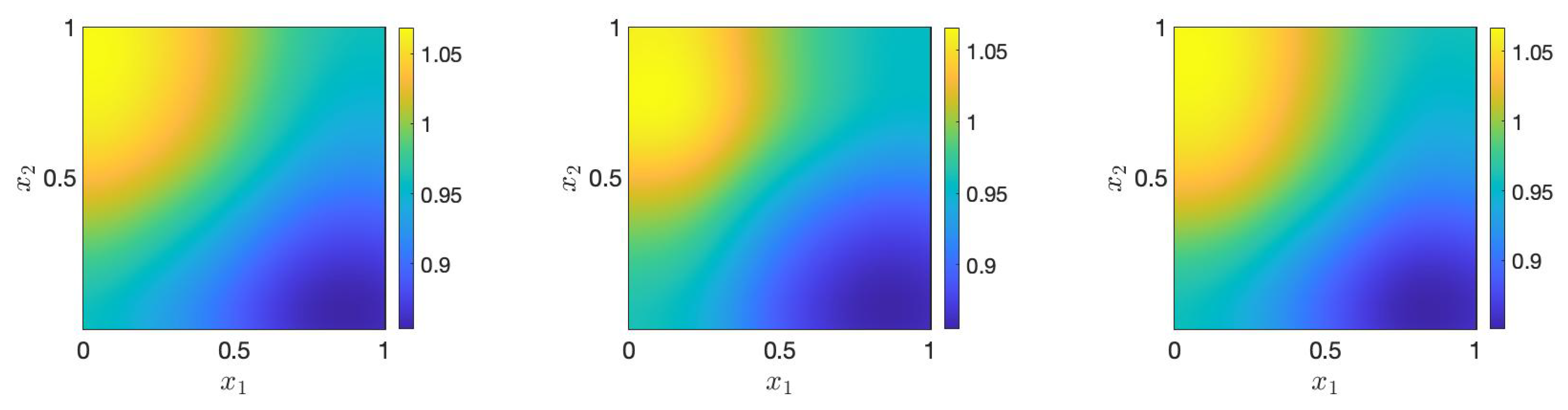
Figure 3 displays the mean of posterior samples generated by full MCMC, prior ANOVA-GP-MCMC, and adaptive ANOVA-GP-MCMC, from which we can observe that the results obtained from the three sets are similar to the ground truth (see Figure 1), indicating the effectiveness of the proposed approach.
Table 3 illustrates the average cost for a single sample in the three sets. The model based on posterior samples accelerates the sampling speed by , evidencing the substantial improvement in efficiency achieved by the proposed method.
To access the accuracy of the estimated posterior mean and variance, we introduce the relative mean error and the relative variance error as
where the mean and variance of the posterior samples are computed through
The reference mean estimate and the reference variance estimate in (53) are obtained by full MCMC with samples.
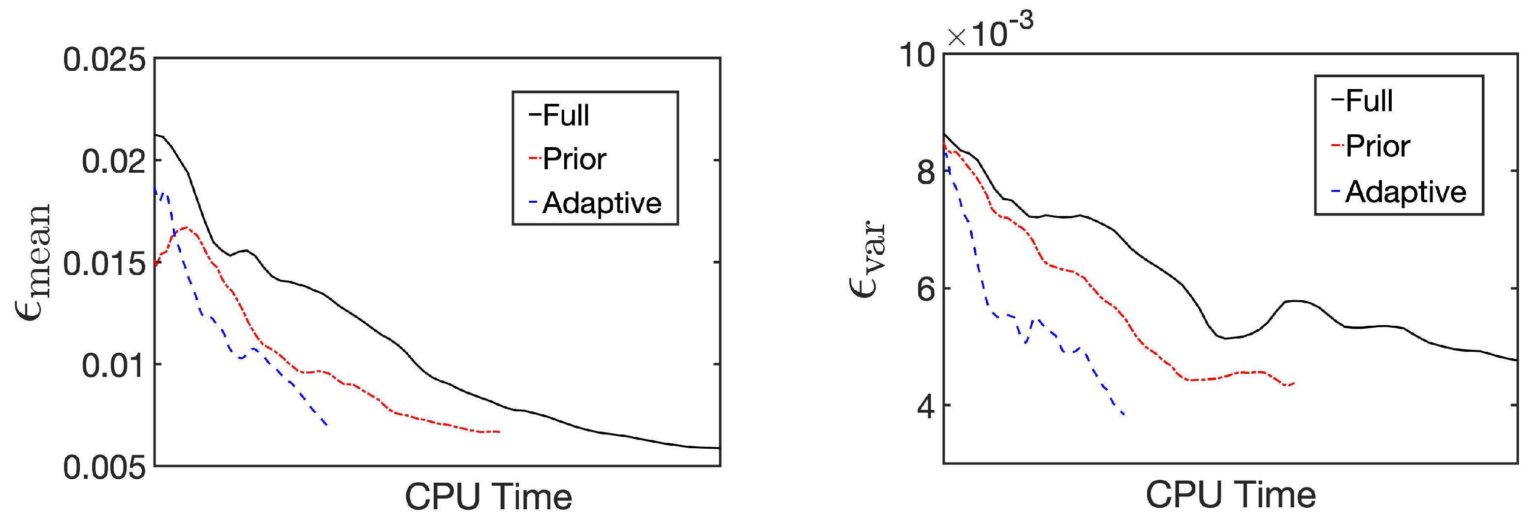
Figure 4 illustrates the trend of and during the sampling process of the three sets. The figure reveals that, owing to the acceleration of individual sampling, the relative error decreases more rapidly using the ANOVA-GP model than with the full model. Particularly in the adaptive ANOVA-GP model, as the anchor point and the samples used for construction are closer to the posterior distribution, fewer ANOVA terms are selected in , and a smaller number of PCA modes remain in each local problem.
Table 4 shows the total number of PCA modes in the model used in prior ANOVA-GP-MCMC (referred to as the prior ANOVA-GP model) and the updating model in adaptive ANOVA-GP-MCMC (referred to as the posterior ANOVA-GP model). Because of the substantial reduction in the cost of a single prediction compared to the prior-based model, adaptive ANOVA-GP-MCMC achieves a given accuracy even more rapidly.
5. Conclusions
In high-dimensional Bayesian inverse problems, establishing a cost-effective surrogate model for the forward model is pivotal for accelerating the MCMC process. Our study leverages ANOVA decomposition and PCA to break down the high-dimensional original problem into several low-dimensional input–output sub-problems. Gaussian process regression is then employed to build local predictors. To enhance the overall efficiency of the model in the Bayesian inversion setting, we propose an adaptive ANOVA-GP-MCMC algorithm that updates the model using posterior samples obtained during the sampling process. Through numerical experiments, we first validate the computational accuracy and efficiency of the ANOVA-GP model. Subsequently, we apply this model to the MCMC process to evaluate the effectiveness of our adaptive algorithm. It is important to note that our study currently focuses on ANOVA decomposition based on a single anchor point: limiting its applicability to Bayesian inverse problems with single-peak posterior distributions. For multi-peak distributions, a potential solution is to employ multiple anchor points for ANOVA decomposition. Additionally, although the number of selected ANOVA terms does not increase exponentially with the growth of the parameter dimension, this method may still lose its acceleration effect when dealing with extremely high-dimensional parameters. Developing a high-dimensional-model reduction method with broader applicability than ANOVA decomposition will be a key focus of our future work.
Author Contributions
Conceptualization, X.S., H.Z. and G.W.; methodology, X.S., H.Z. and G.W.; software, X.S. and H.Z.; validation, X.S., H.Z. and G.W.; investigation, X.S., H.Z. and G.W.; writing—original draft preparation, X.S. and H.Z.; writing—review and editing, X.S., H.Z. and G.W.; visualization, X.S. and H.Z.; project administration, G.W. All authors have read and agreed to the published version of the manuscript.
Funding
This research was funded by the Science and Technology Commission of Shanghai Municipality (STCSM), grant number 22DZ1101200.
Data Availability Statement
Data are contained within the article.
Conflicts of Interest
The authors declare no conflicts of interest.
Abbreviations
The following abbreviations are used in this manuscript:
| ANOVA | Analysis of variance |
| GP | Gaussian process |
| PCA | Principle component analysis |
| MCMC | Markov chain Monte Carlo |
References
- Tarantola, A. Inverse Problem Theory and Methods for Model Parameter Estimation; SIAM: Philadelphia, PA, USA, 2005. [Google Scholar]
- Keilis-Borok, V.; Yanovskaja, T. Inverse problems of seismology (structural review). Geophys. J. Int. 1967, 13, 223–234. [Google Scholar] [CrossRef]
- Beck, J.V. Nonlinear estimation applied to the nonlinear inverse heat conduction problem. Int. J. Heat Mass Transf. 1970, 13, 703–716. [Google Scholar] [CrossRef]
- Wang, J.; Zabaras, N. A Bayesian inference approach to the inverse heat conduction problem. Int. J. Heat Mass Transf. 2004, 47, 3927–3941. [Google Scholar] [CrossRef]
- Luo, C.; Shen, L.; Xu, A. Modelling and estimation of system reliability under dynamic operating environments and lifetime ordering constraints. Reliab. Eng. Syst. Saf. 2022, 218, 108136. [Google Scholar] [CrossRef]
- Wang, W.; Cui, Z.; Chen, R.; Wang, Y.; Zhao, X. Regression analysis of clustered panel count data with additive mean models. Stat. Pap. 2023, 1–22. [Google Scholar] [CrossRef]
- Tarantola, A. Popper, Bayes and the inverse problem. Nat. Phys. 2006, 2, 492–494. [Google Scholar] [CrossRef]
- Robert, C.P.; Casella, G.; Casella, G. Monte Carlo Statistical Methods; Springer: New York, NY, USA, 1999; Volume 2. [Google Scholar]
- Yeh, W.W.G. Review of parameter identification procedures in groundwater hydrology: The inverse problem. Water Resour. Res. 1986, 22, 95–108. [Google Scholar] [CrossRef]
- Virieux, J.; Operto, S. An overview of full-waveform inversion in exploration geophysics. Geophysics 2009, 74, WCC1–WCC26. [Google Scholar] [CrossRef]
- Marzouk, Y.M.; Najm, H.N.; Rahn, L.A. Stochastic spectral methods for efficient Bayesian solution of inverse problems. J. Comput. Phys. 2007, 224, 560–586. [Google Scholar] [CrossRef]
- Wang, H.; Li, J. Adaptive Gaussian process approximation for Bayesian inference with expensive likelihood functions. Neural Comput. 2018, 30, 3072–3094. [Google Scholar] [CrossRef]
- Chen, C.; Liao, Q. ANOVA Gaussian process modeling for high-dimensional stochastic computational models. J. Comput. Phys. 2020, 416, 109519. [Google Scholar] [CrossRef]
- Ma, X.; Zabaras, N. An efficient Bayesian inference approach to inverse problems based on an adaptive sparse grid collocation method. Inverse Probl. 2009, 25, 035013. [Google Scholar] [CrossRef]
- Galbally, D.; Fidkowski, K.; Willcox, K.; Ghattas, O. Non-linear model reduction for uncertainty quantification in large-scale inverse problems. Int. J. Numer. Methods Eng. 2010, 81, 1581–1608. [Google Scholar] [CrossRef]
- Lieberman, C.; Willcox, K.; Ghattas, O. Parameter and state model reduction for large-scale statistical inverse problems. SIAM J. Sci. Comput. 2010, 32, 2523–2542. [Google Scholar] [CrossRef]
- Frangos, M.; Marzouk, Y.; Willcox, K.; van Bloemen Waanders, B. Surrogate and reduced-order modeling: A comparison of approaches for large-scale statistical inverse problems. In Large-Scale Inverse Problems and Quantification of Uncertainty; John Wiley & Sons: Chichester, UK, 2010; pp. 123–149. [Google Scholar]
- Li, J. A note on the Karhunen–Loève expansions for infinite-dimensional Bayesian inverse problems. Stat. Probab. Lett. 2015, 106, 1–4. [Google Scholar] [CrossRef]
- Sobol’, I.M. Theorems and examples on high dimensional model representation. Reliab. Eng. Syst. Saf. 2003, 79, 187–193. [Google Scholar] [CrossRef]
- Gao, Z.; Hesthaven, J.S. On ANOVA expansions and strategies for choosing the anchor point. Appl. Math. Comput. 2010, 217, 3274–3285. [Google Scholar] [CrossRef]
- Elman, H.C.; Liao, Q. Reduced basis collocation methods for partial differential equations with random coefficients. SIAM/ASA J. Uncertain. Quantif. 2013, 1, 192–217. [Google Scholar] [CrossRef]
- Liao, Q.; Li, J. An adaptive reduced basis ANOVA method for high-dimensional Bayesian inverse problems. J. Comput. Phys. 2019, 396, 364–380. [Google Scholar] [CrossRef]
- Ren, O.; Boussaidi, M.A.; Voytsekhovsky, D.; Ihara, M.; Manzhos, S. Random Sampling High Dimensional Model Representation Gaussian Process Regression (RS-HDMR-GPR) for representing multidimensional functions with machine-learned lower-dimensional terms allowing insight with a general method. Comput. Phys. Commun. 2022, 271, 108220. [Google Scholar] [CrossRef]
- Boussaidi, M.A.; Ren, O.; Voytsekhovsky, D.; Manzhos, S. Random sampling high dimensional model representation Gaussian process regression (RS-HDMR-GPR) for multivariate function representation: Application to molecular potential energy surfaces. J. Phys. Chem. A 2020, 124, 7598–7607. [Google Scholar] [CrossRef] [PubMed]
- Metropolis, N.; Rosenbluth, A.W.; Rosenbluth, M.N.; Teller, A.H.; Teller, E. Equation of state calculations by fast computing machines. J. Chem. Phys. 1953, 21, 1087–1092. [Google Scholar] [CrossRef]
- Hastings, W.K. Monte Carlo sampling methods using Markov chains and their applications. Biometrika 1970, 57, 97–109. [Google Scholar] [CrossRef]
- Rabitz, H.; Aliş, Ö.F. General foundations of high-dimensional model representations. J. Math. Chem. 1999, 25, 197–233. [Google Scholar] [CrossRef]
- Ma, X.; Zabaras, N. An adaptive high-dimensional stochastic model representation technique for the solution of stochastic partial differential equations. J. Comput. Phys. 2010, 229, 3884–3915. [Google Scholar] [CrossRef]
- Ki, W.C.; Rasmussen, C.E. Gaussian Processes for Machine Learning; MIT Press: Cambridge, MA, USA, 2006; Volume 14. [Google Scholar]
- Rasmussen, C.E. Gaussian processes in machine learning. In Summer School on Machine Learning; Springer: Berlin/Heidelberg, Germany, 2003; pp. 63–71. [Google Scholar]
- Schulz, E.; Speekenbrink, M.; Krause, A. A tutorial on Gaussian process regression: Modelling, exploring, and exploiting functions. J. Math. Psychol. 2018, 85, 1–16. [Google Scholar] [CrossRef]
- Williams, C.; Rasmussen, C. Gaussian processes for regression. Adv. Neural Inf. Process. Syst. 1995, 8, 514–520. [Google Scholar]
- Chen, Z.; Fan, J.; Wang, K. Remarks on multivariate Gaussian process. arXiv 2020, arXiv:2010.09830. [Google Scholar]
- Li, J.; Marzouk, Y.M. Adaptive construction of surrogates for the Bayesian solution of inverse problems. SIAM J. Sci. Comput. 2014, 36, A1163–A1186. [Google Scholar] [CrossRef]
- Elman, H.C.; Silvester, D.J.; Wathen, A.J. Finite Elements and Fast Iterative Solvers: With Applications in Incompressible Fluid Dynamics; Oxford University Press: Oxford, UK, 2014. [Google Scholar]
- Elman, H.C.; Ramage, A.; Silvester, D.J. IFISS: A computational laboratory for investigating incompressible flow problems. SIAM Rev. 2014, 56, 261–273. [Google Scholar] [CrossRef]
Figure 1.
The FEM grids and sensor locations (left) and the ground truth of the permeability field (right).
Figure 1.
The FEM grids and sensor locations (left) and the ground truth of the permeability field (right).

Figure 2.
The relative errors of ANOVA-GP models when (left), (middle), and (right) for 500 test samples.
Figure 2.
The relative errors of ANOVA-GP models when (left), (middle), and (right) for 500 test samples.

Figure 3.
The means of posterior samples generated by full MCMC (left), prior ANOVA-GP-MCMC (middle), and adaptive ANOVA-GP-MCMC (right).
Figure 3.
The means of posterior samples generated by full MCMC (left), prior ANOVA-GP-MCMC (middle), and adaptive ANOVA-GP-MCMC (right).

Figure 4.
Errors in mean and variance estimates ( and ) for full MCMC, prior ANOVA-GP-MCMC, and adaptive ANOVA-GP-MCMC.
Figure 4.
Errors in mean and variance estimates ( and ) for full MCMC, prior ANOVA-GP-MCMC, and adaptive ANOVA-GP-MCMC.


Table 1.
The mean of relative errors and the mean of prediction costs of ANOVA-GP models when (left), (middle), and (right).
Table 1.
The mean of relative errors and the mean of prediction costs of ANOVA-GP models when (left), (middle), and (right).
| Mean cost (s) | |||
| Mean relative error |
Table 2.
The number of active ANOVA terms at each order when (left), (middle), and (right).
| 12 | 1 | 0 | 0 | 0 | 12 | |
| 12 | 3 | 3 | 0 | 0 | 15 | |
| 12 | 4 | 6 | 3 | 0 | 18 |
Table 3.
The mean costs per sample of full MCMC (left), prior ANOVA-GP-MCMC (middle), and adaptive ANOVA-GP-MCMC (right).
Table 3.
The mean costs per sample of full MCMC (left), prior ANOVA-GP-MCMC (middle), and adaptive ANOVA-GP-MCMC (right).
| Full | Prior | Adaptive | |
|---|---|---|---|
| Cost per sample (s) | |||
| Speedup | ∖ |
Table 4.
The number of total PCA modes in the prior ANOVA-GP model (left) and the posterior ANOVA-GP model (right).
Table 4.
The number of total PCA modes in the prior ANOVA-GP model (left) and the posterior ANOVA-GP model (right).
| Prior ANOVA-GP Model | Posterior ANOVA-GP Model | |
|---|---|---|
| Number of PCA modes | 47 | 29 |
Disclaimer/Publisher’s Note: The statements, opinions and data contained in all publications are solely those of the individual author(s) and contributor(s) and not of MDPI and/or the editor(s). MDPI and/or the editor(s) disclaim responsibility for any injury to people or property resulting from any ideas, methods, instructions or products referred to in the content. |
© 2024 by the authors. Licensee MDPI, Basel, Switzerland. This article is an open access article distributed under the terms and conditions of the Creative Commons Attribution (CC BY) license (https://creativecommons.org/licenses/by/4.0/).
Share and Cite
MDPI and ACS Style
Shi, X.; Zhang, H.; Wang, G. ANOVA-GP Modeling for High-Dimensional Bayesian Inverse Problems. Mathematics 2024, 12, 301. https://0-doi-org.brum.beds.ac.uk/10.3390/math12020301
AMA Style
Shi X, Zhang H, Wang G. ANOVA-GP Modeling for High-Dimensional Bayesian Inverse Problems. Mathematics. 2024; 12(2):301. https://0-doi-org.brum.beds.ac.uk/10.3390/math12020301
Chicago/Turabian StyleShi, Xiaoyu, Hanyu Zhang, and Guanjie Wang. 2024. "ANOVA-GP Modeling for High-Dimensional Bayesian Inverse Problems" Mathematics 12, no. 2: 301. https://0-doi-org.brum.beds.ac.uk/10.3390/math12020301
Note that from the first issue of 2016, this journal uses article numbers instead of page numbers. See further details here.