
Cohen–Macaulayness of Vertex Splittable Monomial Ideals

Department of Mathematics and Computer Sciences, Physics and Earth Sciences, University of Messina, Viale Ferdinando Stagno d’Alcontres 31, 98166 Messina, Italy
*
Author to whom correspondence should be addressed.
†
These authors contributed equally to this work.
‡
These authors are members of GNSAGA of INDAM (Italy).
Mathematics 2024, 12(6), 912; https://0-doi-org.brum.beds.ac.uk/10.3390/math12060912
Submission received: 8 February 2024
/
Revised: 12 March 2024
/
Accepted: 16 March 2024
/
Published: 20 March 2024
(This article belongs to the Special Issue Combinatorics and Computation in Commutative Algebra)
Abstract
:In this paper, we give a new criterion for the Cohen–Macaulayness of vertex splittable ideals, a family of monomial ideals recently introduced by Moradi and Khosh-Ahang. Our result relies on a Betti splitting of the ideal and provides an inductive way of checking the Cohen–Macaulay property. As a result, we obtain characterizations for Gorenstein, level and pseudo-Gorenstein vertex splittable ideals. Furthermore, we provide new and simpler combinatorial proofs of known Cohen–Macaulay criteria for several families of monomial ideals, such as (vector-spread) strongly stable ideals and (componentwise) polymatroidals. Finally, we characterize the family of bi-Cohen–Macaulay graphs by the novel criterion for the Cohen–Macaulayness of vertex splittable ideals.
Keywords:
minimal resolutions; graded Betti numbers; Betti splittings; Cohen–Macaulay ideals; vertex splittable idealsMSC:
13D02; 13F20; 13H10; 13F55; 05C751. Introduction
Let be the polynomial ring with coefficients in a field K. In [1], Moradi and Khosh-Ahang introduced the notion of a vertex splittable ideal, an algebraic analog of the vertex decomposability property of a simplicial complex. In more detail, let be a simplicial complex and let F be a face of . One can associate with two special simplicial complexes: the deletion of F, defined as , and the link of F, defined as . For , one sets and . The notion of vertex decomposition was introduced by Provan and Billera [2] for a pure simplicial complex, and afterwards, it was extended to nonpure complexes by Bjoner and Wachs [3]. A vertex decomposable simplicial complex is recursively defined as follows: is a simplex or has some vertex x such that (1) both and are vertex decomposable, and (2) there is no face of which is also a facet of . An ideal I of S is called vertex decomposable if , with being a vertex decomposable simplicial complex. We recall that is the Stanley–Reisner ideal of over K, that is, the ideal of S generated by the squarefree monomial , for all . It is well-known that for a simplicial complex , the following implications hold: vertex decomposable ⇒ shellable ⇒ sequentially Cohen–Macaulay (see, for instance, [4]). Moreover, there exist characterizations of shellable, sequentially Cohen–Macaulay and Cohen–Macaulay complexes via the Alexander dual ideals (see [5] [Theorem 1.4], [6] [Theorem 2.1], [7] [Theorem 3], respectively), where is the Alexander dual simplicial complex associated with .
Inspired by the above results, in [1], Moradi and Khosh-Ahang asked and solved the following question: Is it possible to characterize a vertex decomposable simplicial complex Δ by means of ? For this aim, they introduced the notion of the vertex splittable monomial ideal (Definition 1) and proved that a simplicial complex is vertex decomposable if and only if is a vertex splittable ideal [1] [Theorem 2.3]. Moreover, the authors in [1] proved that a vertex splittable ideal has a Betti splitting (see Definition 2 and Theorem 1).
Determining when a monomial ideal is Cohen–Macaulay is a fundamental and challenging problem in commutative algebra. Motivated by this and the results of [1], in this paper, we tackle the Cohen–Macaulayness of vertex splittable ideals. Our main contribution (Theorem 2) is a new characterization of the Cohen–Macaulayness of a vertex splittable ideal in terms of a Betti splitting. This new criterion provides a neat and effective inductive strategy to determine when a vertex splittable ideal is Cohen–Macaulay.
This article is organized as follows. In Section 2.2, we recall relevant definitions and auxiliary results that we will use later on. In Section 3, we state a new criterion for the Cohen–Macaulayness of vertex splittable ideals (Theorem 2). As a consequence, we obtain characterizations for Gorenstein, level and pseudo-Gorenstein Cohen–Macaulay vertex splittable ideals (Corollary 1). The results in this section will be used in the subsequent section (Section 4), where we recover some interesting Cohen–Macaulay classifications of families of monomial ideals: (vector-spread) strongly stable ideals and (componentwise) polymatroidal ideals. Moreover, a new characterization of bi-Cohen–Macaulay graphs is presented (Theorem 6). Finally, Section 5 contains our conclusions and perspectives.
2. Preliminaries
In this section, we recall the basic notions and notations we will use in the body of the paper [1,8].
Let be a polynomial ring in n variables over a field K with the standard grading, i.e., each . For any finitely generated graded S-module M, there exists the unique minimal graded free S-resolution
with . The numbers are called the graded Betti numbers of M, while are called the total Betti numbers of M. Recall that the projective dimension and the Castelnuovo–Mumford regularity of M are defined as follows:
More precisely, the projective dimension is the length of a minimal graded free resolution of the finitely generated graded S-module M.
2.1. Cohen–Macaulay Property
In this subsection, we introduce the notion of the Cohen–Macaulay ring and some related notions.
Firstly, let be the unique maximal homogeneous ideal of S, and let M be a finitely generated graded S-module M.
A sequence of homogeneous elements of is called an M-sequence if the following criteria are met:
- (1)
- the multiplication map is injective for all i.
- (2)
- .
The length of a maximal homogeneous M-sequence is called the depth of M. By the Auslander–Buchsbaum formula (see, for instance, [9]), we have
A finitely generated graded S-module M is called a Cohen–Macaulay module (CM module for short) if , where is the Krull dimension of M [9]. Let I be a graded ideal of S; the graded ring is said to be CM if , viewed as an S-module, is CM. The graded ideal I is called a CM ideal.
Let be a graded CM ideal, and let be the projective dimension of . The Cohen–Macaulay type (CM type for short) of is defined as the integer . It is well-known that is Gorenstein if and only if . We say that I is Gorenstein if is such.
2.2. Vertex Splittable Monomial Ideals
In this subsection, we discuss the notions of vertex splittable monomial ideals and of Betti splittings.
Let be a monomial ideal. We denote by the unique minimal monomial generating set of I. We recall the following notion [1] [Definition 2.1].
Definition 1.
The ideal I is called vertex splittable if it can be obtained by the following recursive procedure:
- (i)
- If u is a monomial and , or , then I is vertex splittable.
- (ii)
- If there exists a variable and vertex splittable ideals andsuch that , and is the union of and , then I is vertex splittable.In this case, we say that is a vertex splitting of I and is a splitting vertex of I.
Remark 1.
One can observe that while in general, the Cohen–Macaulayness of depends on the field K ([9] (p. 236)), if I is a vertex splittable ideal, then this is not the case. Indeed, the Krull dimension of , where I is a monomial ideal, does not depend on K. Furthermore, by [1] [Theorem 2.4], vertex splittable ideals have linear quotients. Hence, is also independent from K.
In [8], the next concept was introduced.
Definition 2.
Let I, J, L be monomial ideals of S such that is the disjoint union of and . We say that is a Betti splitting if
When is a Betti splitting, important homological invariants of the ideal I are related to the invariants of the smaller ideals J and L. Indeed, in [8] [Corollary 2.2], it is proved that if is a Betti splitting, then
We quote the next crucial result from [1].
Theorem 1
([1] [Theorem 2.8]). Let be a vertex splitting for the monomial ideal I of S. Then is a Betti splitting.
We close this subsection by introducing two families of monomial ideals: the t-spread strongly stable ideals and the (componentwise) polymatroidal ideals. We will show in Section 4 that they are families of vertex splittable ideals (see Propositions 1 and 2).
A very meaningful class of monomial ideals of the polynomial ring S is the class of strongly stable monomial ideals. They are fundamental in commutative algebra, because if K has the characteristic zero, then they appear as generic initial ideals [16]. In [17], the concept of a strongly stable ideal was generalized to that of the -spread strongly stable ideal.
Let , be a tuple, and let be a monomial, with and . We say that u is -spread if
A monomial ideal is called -spread if consists of -spread monomials. A -spread ideal is called -spread strongly stable if for all -spread monomials and all such that divides u and is -spread, then . For and , we obtain the strongly stable and the squarefree strongly stable ideals [13].
Another fundamental family of monomial ideals of S is that of the so-called polymatroidal ideals.
Let be a monomial ideal generated in a single degree. We say that I is polymatroidal if the set of the exponent vectors of the minimal monomial generators of I is the set of bases of a discrete polymatroid [13].
Polymatroidal ideals are characterized by the exchange property [13] [Theorem 2.3]. For a monomial , let
Lemma 1.
Let be a monomial ideal generated in a single degree. Then I is polymatroidal if and only if the following exchange property holds: for all and all i such that , there exists j with such that .
An arbitrary monomial ideal I is called componentwise polymatroidal if the component is polymatroidal for all j. Here, for a graded ideal and an integer j, we denote by the graded ideal generated by all polynomials of degree j belonging to J.
Polymatroidal ideals are vertex splittable [18] [Lemma 2.1]. In Proposition 2, we prove the analogous case for componentwise polymatroidal ideals.
3. A Cohen–Macaulay Criterion
In this section, we introduce a new criterion for the Cohen–Macaulayness of vertex splittable ideals. As a result, we obtain characterizations for Gorenstein, level and pseudo-Gorenstein vertex splittable ideals.
The main result in the section is the following.
Theorem 2.
Let be a vertex splittable monomial ideal such that , and let be a splitting vertex of I. Then, the following conditions are equivalent:
- (a)
- I is CM.
- (b)
- are CM, and .
Proof.
We may assume . Let be the vertex splitting of I. Since is a Betti splitting (Theorem 1), then Formula (3) together with the Auslander–Buchsbaum Formula (1), implies
Notice that and , because and does not divide any minimal monomial generator of . Consequently, , and so
We have the short exact sequence
Notice that , because does not divide any minimal monomial generator of and . Since , we have . Thus, . Moreover, , and so we obtain the short exact sequence
Hence, . Since , we obtain that . Hence,
Hence, , are CM and .
(b)⇒(a) Conversely, assume that and are CM and that . Then,
and
The next important vanishing theorem due to Grothendieck [9] [Theorem 3.5.7] will be crucial to characterize Gorenstein, level and pseudo-Gorenstein vertex splittable ideals. If is a Noetherian local ring and M a finitely generated R-module, we denote by the ith local cohomology module of M with support on [9].
Theorem 3.
Let be a Noetherian local ring and M a finitely generated R-module of depth t and dimension d. Then
- (a)
- for and .
- (b)
- and .
Corollary 1.
Let be a vertex splittable CM ideal such that , and let be a vertex splitting of I. Then, the following statements hold:
- (a)
- .
- (b)
- is Gorenstein if and only if I is a principal ideal.
- (c)
- is level if and only if and are level and .
- (d)
- is pseudo-Gorenstein if and only if one of the following occurs: Either is pseudo-Gorenstein and or is pseudo-Gorenstein and .
- (e)
- .
Proof.
We may assume that . Since is CM, Theorem 2 guarantees that are CM and . Hence, . Let . In particular, we have . Now, by [1] [Remark 2.10], we have for all j
Since , the above formula simplifies to
From this formula, we deduce that
We obtain the following:
(a) The assertion follows immediately from (6).
(b) In the proof of Theorem 2 we noted, that . Thus, . By (a), it follows that I is Gorenstein if and only if is Gorenstein, and . Using Formula (4) and Theorem 2 (b), we obtain . Since , we have , equivalent to saying that I is a principal ideal.
(c) Assume that is level. Then only for . Since and are both nonzero, we deduce from Formula (6) that and that , are level. Conversely, if and , are level, we deduce from Formula (6) that is level.
(d) Assume that is pseudo-Gorenstein. Then . Since and are both nonzero, we deduce from Formula (6) that either is pseudo-Gorenstein and or is pseudo-Gorenstein and . The converse can be proved in a similar way.
(e) Since is CM, Theorem 2 implies that and are CM and . As shown in the proof of Theorem 2, we have the short exact sequence
This sequence induces the long exact sequence of local cohomology modules:
Let M be a finitely generated CM S-module. By Theorem 3, if and only if . Thus, the above exact sequence simplifies to
and the assertion follows. □
Remark 2.
It is clear that any ideal generated by a subset of the variables of S is Gorenstein and vertex splittable. Hence, Corollary 1 implies immediately that the only Gorenstein vertex splittable ideals of S are the principal monomial ideals and the ideals generated by a subset of the variables.
4. Families of Cohen–Macaulay Vertex Splittable Ideals
In this section, by using Theorem 2, we recover in a simple and very effective manner Cohen–Macaulay criteria for several families of monomial ideals. We use the fact that if is a vertex splitting, then are vertex splittable ideals that, in good cases, belong again to a given family of vertex splittable monomial ideals and to which one may apply inductive arguments.
The first two families were introduced in Section 2.2.
4.1. (Vector-Spread) Strongly Stable Ideals
In [19] [Theorem 4.3], we classified the CM -spread strongly stable ideals. Here, we recover this result using Theorem 2.
Proposition 1.
Let be a -spread strongly stable ideal such that . Then
- (a)
- I is vertex splittable;
- (b)
- I is CM if and only if there exists such that
Proof.
(a) We proceed by double induction on the number of variables n and the highest degree d of a generator . If , then I is a principal ideal whether or not the integer d is, and so it is vertex splittable. Suppose . If , then I is an ideal generated by a subset of the variables and it is clearly vertex splittable. Suppose . We can write , where and . It is immediately clear that is -spread strongly stable and that is a -spread strongly stable ideal of . By induction on n and d, we have that and are vertex splittable. Hence, so is I.
(b) We may suppose that divides some minimal generator of I. Otherwise, we can consider I as a monomial ideal of a smaller polynomial ring. If I is principal, then we have , with , and . Otherwise, if I is not principal, then , and we can write as above. By Theorem 2, is CM and . Thus, . Hence, by induction, there exists such that
Since , the assertion follows. □
4.2. Componentwise Polymatroidal Ideals
In this subsection, we prove that componentwise polymatroidal ideals are also vertex splittable.
A longstanding conjecture of Bandari and Herzog predicted that componentwise polymatroidal ideals have linear quotients [20]. This conjecture was solved recently in [21] [Theorem 3.1]. Inspecting the proof of this theorem, we obtain the following:
Proposition 2.
Componentwise polymatroidal ideals are vertex splittable.
Proof.
Let be a componentwise polymatroidal ideal. We prove the statement by induction on . We may assume that all variables divide some minimal monomial generator of I. Moreover, it holds that for any variable which divides a minimal monomial generator of minimal degree of I, we can write , where , and the following properties are satisfied (see the proof of [21] [Theorem 3.1]):
- (i)
- as monomial ideals of S.
- (ii)
- is a componentwise polymatroidal ideal of S.
- (iii)
- is a componentwise polymatroidal ideal of .
By induction, it follows that both and are vertex splittable. Hence, so is I. □
We have the following corollary.
Corollary 2.
Let be a componentwise polymatroidal ideal and let be any variable dividing some minimal monomial generator of least degree of I. Suppose that . Then, the following conditions are equivalent.
- (a)
- I is CM.
- (b)
- are CM componentwise polymatroidal ideals and .
Moreover, if is a polymatroidal ideal generated in degree and is a variable dividing some monomial of , then is polymatroidal. And, in addition, if I is CM, then is also CM.
Proof.
It follows by combining the vertex splitting presented in the proof of Proposition with the facts (ii) and (iii) and with Theorem 2. For the last statement, see [22] [Lemma 5.6]. □
At the moment, to classify all CM componentwise polymatroidal ideals seems a hopeless task. For instance, let J be any componentwise polymatroidal ideal. Let ℓ be the highest degree of a minimal monomial generator of J, and let be any integer. It is easy to see that is componentwise polymatroidal. Since , then is automatically CM.
Example 1.
Consider the ideal of , see [21] [Example 3.2]. One can easily check that I is a CM componentwise polymatroidal ideal. Indeed, it is not difficult to check that is polymatroidal for . For , the ideal is polymatroidal because it is the product of two polymatroidal ideals [16] [Theorem 12.6.3]. Notice that in this case, .
Nonetheless, if I is generated in a single degree, that is, if I is actually polymatroidal, then Herzog and Hibi [23] [Theorem 4.2] showed that I is CM if and only if (i) I is a principal ideal, (ii) I is a squarefree Veronese ideal , that is, it is generated by all squarefree monomials of S of a given degree , or (iii) I is a Veronese ideal, that is, for some integer .
The proof presented by Herzog and Hibi is based on the computation of . We now present a different proof based on the criterion for Cohen–Macaulayness proved in Theorem 2.
Corollary 3.
A polymatroidal is CM if and only if I is one of the following:
- (a)
- A principal ideal.
- (b)
- A Veronese ideal.
- (c)
- A squarefree Veronese ideal.
For the proof, we need the following well-known identities. For the convenience of the reader, we provide a proof that uses the vertex splittings technique.
Lemma 2.
Let be positive integers. Then
Proof.
Since , we have and . If , then and . If , we notice that is a vertex splitting. By Formula (4) and induction on n and d,
as wanted.
□
We are now ready for the proof of Corollary 3.
Proof of Corollary 3.
Let I be a polymatroidal ideal. We proceed by induction on . If , then I is principal and it is CM. Now, let . If , then I is CM. Thus, we assume that I is generated in degree , that all variables divide some minimal monomial generator of I and that the greatest common divisor of the minimal monomial generators of I is one. By Proposition 2 and Corollary 2, we have a vertex splitting for each variable and are CM polymatroidal ideals with . Thus, . We may assume that .
Since are strictly less than , by induction, it follows that is either a principal ideal, a Veronese ideal or a squarefree Veronese ideal, and the same possibilities occur for . We distinguish the various possibilities.
- Case 1.
- Let be a principal ideal, then . Thus, .
Under this assumption, cannot be principal because .
Assume that is a Veronese ideal in m variables. Since all variables of S divide some monomial of and , then or , where and . Thus, or . Lemma 2 implies . So, or .
If , then , which is CM and Veronese, or , which is not CM.
Otherwise, if , then or else where is a monomial of degree d. If , then one easily sees that only in the second case and for we have that I is a CM polymatroidal ideal, which is the squarefree Veronese . Otherwise, suppose . We may assume that divides u. In the first case, is not principal, nor Veronese, nor squarefree Veronese. Thus, by induction, is not a CM polymatroidal ideal, and by Corollary 2, we deduce that I is also not CM. Similarly, in the second case, we see that , and thus also I, is not a CM polymatroidal ideal.
Assume now that is a squarefree Veronese ideal in m variables. Then as argued in the case 1.2 we have or . Lemma 2 gives . Thus, . Hence or . So or where is a monomial of degree in the first case or in the second case. In the first case there is i such that divides u. Say . Then is not a principal ideal, neither a Veronese ideal, neither a squarefree Veronese. Therefore, by induction we see that is not a CM polymatroidal ideal, and by Corollary 2 I is also not a CM polymatroidal ideal. Similarly, in the second case, if , then is a CM squarefree Veronese ideal. Otherwise, , say with , divides u, and then, arguing as before, we see that I is not a CM polymatroidal ideal.
- Case 2.
- Let be a Veronese ideal in m variables, then .
Under this assumption, cannot be principal because .
Assume that is a Veronese ideal in ℓ variables. Then or . Lemma 2 implies that . Thus, and or and . In the first case, is a CM Veronese ideal. In the second case, up to relabeling, we can write . However, this ideal is not polymatroidal. Otherwise, by the exchange property (Lemma 1) applied to and , we should have , which is not the case.
Assume now that is a squarefree Veronese ideal in ℓ variables.Then or . Lemma 2 implies that . Thus, either or . Up to relabeling, we have either or . If , then these ideals become either , which is a CM Veronese ideal, or , which is not polymatroidal because the exchange property does not hold for and since . If , then the above ideals are not polymatroidal. In the first case, the exchange property does not hold for and , otherwise for some , which is not the case.
- Case 3.
- Let be a squarefree Veronese in m variables, . Then Lemma 2 implies with . Hence, .
In such a case, the ideal cannot be principal because .
Assume that is a Veronese ideal in ℓ variables. Then or . Lemma 2 implies that . Hence, either or . Since , either or . Only the case is possible. If , then and we have . This ideal is not CM, otherwise it would be height-unmixed. Indeed, and are two associated primes of I having different heights.
Finally, assume that is a squarefree Veronese ideal in ℓ variables. Then or . Lemma 2 implies that . Thus, and so either or . The first case is impossible because . In the second case, we have which is a CM squarefree Veronese ideal. □
4.3. Bi-Cohen–Macaulay Graphs
Let be a squarefree monomial ideal. Then I may be seen as the Stanley–Reisner ideal of a unique simplicial complex on the vertex set . Attached to I is the Alexander dual , which is again a squarefree monomial ideal. We say that I is bi-Cohen–Macaulay (bi-CM for short) if both I and are CM. By the Eagon–Reiner criterion [16] [Theorem 8.1.9], I has a linear resolution if and only if is CM. Hence, I is bi-CM if and only if it is CM with linear resolution.
Let G be a finite simple graph on the vertex set with edge set . The edge ideal of G is the squarefree monomial ideal of S generated by the monomials with [4]. The Alexander dual of is the squarefree monomial ideal of S generated by the squarefree monomial such that is a minimal vertex cover of G [4]. Such an ideal is denoted by and, since its definition, it is often called the cover ideal of G.
We say that G is a bi-CM graph if is bi-CM.
Let G be a graph. The open neighborhood of is the set
A graph G is called chordal if it has no induced cycles of a length bigger than three. A perfect elimination order of G is an ordering of its vertex set such that induces a complete subgraph on , where is the induced subgraph of G on the vertex set . Hereafter, if is a perfect elimination order of G, we highlight it by . For a complete graph G, we mean a graph satisfying the property that every set with , is an edge of G.
Theorem 4
([24]). A finite simple graph G is chordal if and only if G admits a perfect elimination order.
The edge ideals with linear resolution were classified by Fröberg [25]. Recall that the complementary graph of G is the graph with vertex set and where is an edge of if and only if . A graph G is called cochordal if and only if is chordal.
Theorem 5
([25] [Theorem 1]). Let G be a finite simple graph. Then has a linear resolution if and only if G is cochordal.
We quote the next fundamental result which was proved by Moradi and Khosh-Ahang [1] [Theorem 3.6, Corollary 3.8].
Proposition 3.
Let G be a finite simple graph. Then has linear resolution if and only if is vertex splittable. Furthermore, if is a perfect elimination order of , then
is a vertex splitting of .
Combining the above result with Theorem 2, we obtain the next characterization of the bi-CM graphs.
Theorem 6.
For a finite simple graph G, the following conditions are equivalent.
- (a)
- G is a bi-CM graph.
- (b)
- is a chordal graph with perfect elimination order andfor all such that .
In particular, if any of the equivalent conditions hold, then
for any such that .
Proof.
We proceed by induction on . By Theorem 5, G must be cochordal. Fix , which is a perfect elimination order of . By Proposition 3, is a vertex splitting. Applying Theorem 2, is CM if and only if and are CM and . J is CM because it is an ideal generated by variables and . Notice that is a perfect elimination order of .
If , then and is principal, say . In this case, the thesis holds.
Suppose now that . Then, by induction on n, is CM if and only if
for all such that and moreover
for any such that .
Notice that for all . Thus, by combining (7) and (8) with the equality , we see that is CM if and only if
for all such that .
Thus, we deduce that for all such that , as desired. The inductive proof is complete. □
Notice that in the above characterization, the field K plays no role. In other words, the bi-CM property of edge ideals does not depend on the field K. This also follows from the work of Herzog and Rahimi [26] [Corollary 1.2 (d)], where other classifications of the bi-CM graphs are given.
We end this paper with a couple of examples of a bi-CM and a non-bi-CM graph.
Examples 1.
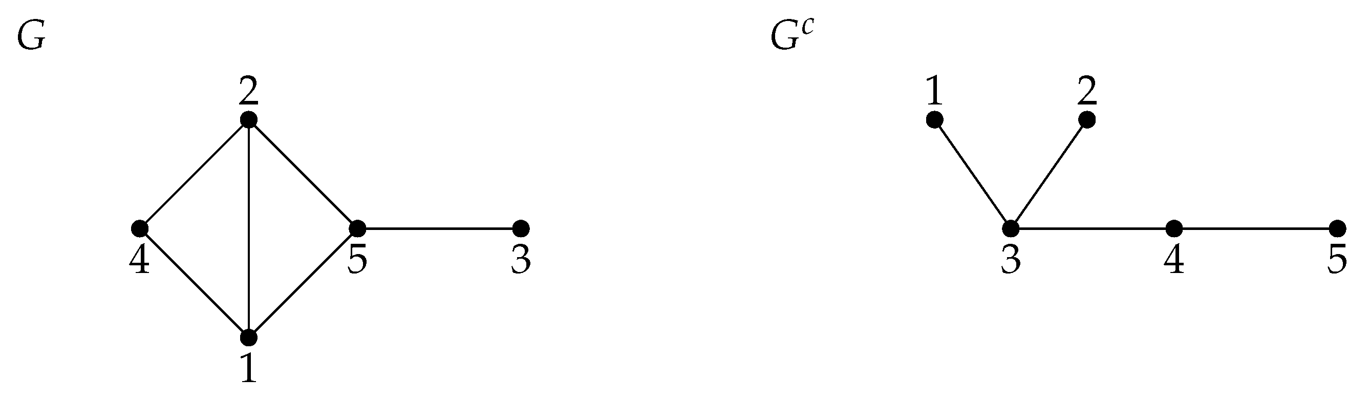
(a) Consider the graph G on five vertices and its complementary graph depicted below in Figure 1.
Notice that is a perfect elimination order of , so that is chordal (Theorem 4). We have only for . It is easy to see that condition (b) of Theorem 6 is verified. Hence G is bi-CM, as one can also verify by using Macaulay2 [27].
- (b)
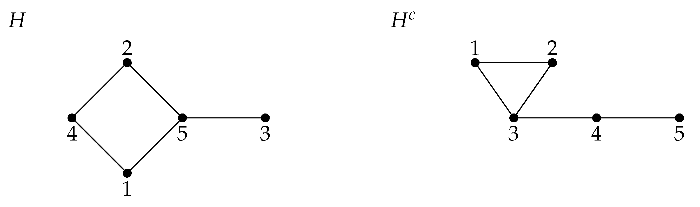
- Consider the graph H and its complementary graph depicted below in Figure 2.
As before, is a perfect elimination order of , and is chordal. We have only for . However, condition (b) of Theorem 6 is not verified. Indeed,
but . Hence, H is not bi-CM. We can also verify this by using Macaulay2 [27]. Indeed , the cover ideal of H, is not CM.
5. Conclusions and Perspectives
In view of our main Theorem 2, one can ask for a similar criterion for the sequentially Cohen–Macaulayness of vertex splittable monomial ideals.
Question 1.
Let be a vertex splittable ideal, and let be a vertex splitting of I. Can we characterize the sequentially Cohen–Macaulayness of I in terms of and ?
This question could have interesting consequences for the theory of polymatroidal ideals. Indeed, a classification of the sequentially Cohen–Macaulay polymatroidal ideals has long been elusive.
On the computational side, to check if a monomial ideal is vertex splittable is far easier than to check if it admits a Betti splitting. Indeed, it is enough to check recursively Definition 1. It could be useful to write a package in Macaulay2 [27] that checks the vertex splittable property and some related properties.
Author Contributions
All authors have made the same contribution. All authors have read and agreed to the published version of the manuscript.
Funding
This research received no external funding.
Data Availability Statement
Data are contained within the article.
Acknowledgments
We thank the anonymous referees for their careful reading and suggestions that improve the quality of the paper.
Conflicts of Interest
The authors declare no conflicts of interest.
References
- Moradi, S.; Khosh-Ahang, F. On vertex decomposable simplicial complexes and their Alexander duals. Math. Scand. 2016, 118, 43–56. [Google Scholar] [CrossRef]
- Provan, J.S.; Billera, L.J. Decompositions of simplicial complexes related to diameters of convex polyhedra. Math. Oper. Res. 1980, 5, 576–594. [Google Scholar] [CrossRef]
- Björner, A.; Wachs, L. Wachs, Shellable nonpure complexes and posets, II. Trans. Amer. Math. Soc. 1997, 349, 3945–3975. [Google Scholar] [CrossRef]
- Villarreal, R.H. Monomial Algebras, 2nd ed.; Monographs and Research Notes in Mathematics; CRC Press: Boca Raton, FL, USA, 2015. [Google Scholar]
- Herzog, H.; Hibi, T.; Zheng, X. Dirac’s theorem on chordal graphs and Alexander duality. Eur. J. Comb. 2004, 25, 949–960. [Google Scholar] [CrossRef]
- Herzog, H.; Hibi, T. Componentwise linear ideals. Nagoya Math. J. 1999, 153, 141–153. [Google Scholar] [CrossRef]
- Eagon, J.; Reiner, V. Resolutions of Stanley-Reisner rings and Alexander duality. J. Pure Appl. Algebra 1998, 130, 265–275. [Google Scholar] [CrossRef]
- Francisco, C.A.; Ha, H.T.; Van Tuyl, A. Splittings of monomial ideals. Proc. Amer. Math. Soc. 2009, 137, 3271–3282. [Google Scholar] [CrossRef]
- Bruns, W.; Herzog, J. Cohen–Macaulay Rings; Cambridge University Press: Cambridge, UK, 1998. [Google Scholar]
- Herzog, H.; Hibi, T.; Ohsugi, H. Binomial Ideals; Graduate Texts in Mathematics; Springer: Cham, Switzerland, 2018; Volume 279. [Google Scholar]
- Ene, V.; Herzog, J.; Hibi, T.; Saeedi Madani, S. Pseudo-Gorenstein and level Hibi rings. J. Algebra 2015, 431, 138–161. [Google Scholar] [CrossRef]
- Ene, V.; Herzog, J. Gröbner Bases in Commutative Algebra; Graduate Studies in Mathematics; American Mathematical Society: Providence, RI, USA, 2011; Volume 130. [Google Scholar]
- Herzog, H.; Hibi, T. Discrete polymatroids. J. Algebr. Combin. 2002, 16, 239–268. [Google Scholar] [CrossRef]
- Deshpande, P.; Roy, A.; Singh, A.; Van Tuyl, A. Fröberg’s Theorem, vertex splittability and higher independence complexes. arXiv 2023, arXiv:2311.02430. [Google Scholar]
- Moradi, S. Normal Rees algebras arising from vertex decomposable simplicial complexes. arXiv 2023, arXiv:2311.15135. [Google Scholar]
- Herzog, H.; Hibi, T. Monomial Ideals; Graduate Texts in Mathematics; Springer: Berlin/Heidelberg, Germany, 2011; Volume 260. [Google Scholar]
- Ficarra, A. Vector-spread monomial ideals and Eliahou–Kervaire type resolutions. J. Algebra 2023, 615, 170–204. [Google Scholar] [CrossRef]
- Mafi, A.; Naderi, D.; Saremi, H. Vertex decomposability and weakly polymatroidal ideals. arXiv 2022, arXiv:2201.06756. [Google Scholar]
- Crupi, M.; Ficarra, A. Minimal resolutions of vector-spread Borel ideals. Analele Stiintifice Ale Univ. Ovidius Constanta Ser. Mat. 2023, 31, 71–84. [Google Scholar]
- Bandari, S.; Herzog, J. Monomial localizations and polymatroidal ideals. Eur. J. Combin. 2013, 34, 752–763. [Google Scholar] [CrossRef]
- Ficarra, A. Shellability of componentwise discrete polymatroids. arXiv 2023, arXiv:2312.13006. [Google Scholar]
- Ficarra, A. Simon’s conjecture and the v-number of monomial ideals. arXiv 2023, arXiv:2309.09188. [Google Scholar]
- Herzog, H.; Hibi, T. Cohen-Macaulay polymatroidal ideals. Eur. J. Combin. 2006, 27, 513–517. [Google Scholar] [CrossRef]
- Dirac, G.A. On rigid circuit graphs. In Abhandlungen aus dem Mathematischen Seminar der Universität Hamburg; Springer: Berlin/Heidelberg, Germany, 1961; Volume 38, pp. 71–76. [Google Scholar]
- Fröberg, R. On Stanley-Reisner rings. In Topics in Algebra; Part 2 (Warsaw, 1988); Banach Center Publications: Warszawa, Poland, 1990; pp. 57–70. [Google Scholar]
- Herzog, J.; Rahimi, A. Bi-Cohen–Macaulay graphs. Electron. J. Combin. 2016, 23, #P1.1. [Google Scholar] [CrossRef] [PubMed]
- Grayson, D.R.; Stillman, M.E. Macaulay2, a Software System for Research in Algebraic Geometry. Available online: http://www.math.uiuc.edu/Macaulay2 (accessed on 5 February 2024).
Figure 1.
A bi-CM graph.

Figure 2.
A not bi-CM graph.

Disclaimer/Publisher’s Note: The statements, opinions and data contained in all publications are solely those of the individual author(s) and contributor(s) and not of MDPI and/or the editor(s). MDPI and/or the editor(s) disclaim responsibility for any injury to people or property resulting from any ideas, methods, instructions or products referred to in the content. |
© 2024 by the authors. Licensee MDPI, Basel, Switzerland. This article is an open access article distributed under the terms and conditions of the Creative Commons Attribution (CC BY) license (https://creativecommons.org/licenses/by/4.0/).
Share and Cite
MDPI and ACS Style
Crupi, M.; Ficarra, A. Cohen–Macaulayness of Vertex Splittable Monomial Ideals. Mathematics 2024, 12, 912. https://0-doi-org.brum.beds.ac.uk/10.3390/math12060912
AMA Style
Crupi M, Ficarra A. Cohen–Macaulayness of Vertex Splittable Monomial Ideals. Mathematics. 2024; 12(6):912. https://0-doi-org.brum.beds.ac.uk/10.3390/math12060912
Chicago/Turabian StyleCrupi, Marilena, and Antonino Ficarra. 2024. "Cohen–Macaulayness of Vertex Splittable Monomial Ideals" Mathematics 12, no. 6: 912. https://0-doi-org.brum.beds.ac.uk/10.3390/math12060912
Note that from the first issue of 2016, this journal uses article numbers instead of page numbers. See further details here.