1. Introduction
In geology, seismometric time-series play the important role of understanding the local structure of the earth. In particular, the manner in which the wave passes through a particular location provides clues on the earth nature. The applications of this knowledge have been used in understanding earthquakes and for other applications in geology like mining for minerals. While siesmometric time series have been studied in many ways, to our knowledge, no academic work looks at the possible knowledge that may be extracted by applying advanced mathematical and statistical interpolation methods to such data. Seismometric time series also present the challenge that they do not have cyclical patterns nor trend in them. The renewed interest in analyzing “critical value phenomena” was discussed in ([
1]). The authors applied powerful modeling techniques to predict major-events (in this case a major earthquake or a financial market crash) efficiently, whereas in reference ([
2]), the article applied the famous Ornstein-Uhlenbeck method to the geophysical data.
In this work, we explore the application of a number of mathematical interpolation techniques to one-dimensional siesmometric time series data, and we study the local variation in the time series. We also apply statistical curve fitting methods to see how this structure can be extracted from our data. In [
3,
4], the authors have applied local regression models and spline interpolation techniques to earthquake geophysical data obtaining promising results.
Our data stems from geologic time series measurements conducted during the Asarco tower demolitions conducted in El Paso, Texas. As explosions were used to demolish the old Asarco smoke stacks, the explosions leaded to a seismic wave which traveled many miles. This wave was measured as the vertical displacement of the ground at the location. While there were multiple explosions and many locations at which the wave was measured, in this paper, we concentrate on a one minute period at six locations. We first apply a number of mathematical interpolation approaches to the data. Next, we study the pattern of location variation of the wave using statistical smoothing approaches.
In addition to the mathematical interpolation of the observed data, we study the local variation of the wave using statistical smoothing techniques. In our approach, we first compute a moving standard deviation filter for the original time series. This filter reflects the local variation of the series, a measure of the wave amplitude at a point in time.
In
Section 2 we describe the data.
Section 3 is devoted to discuss the theoretical aspects of the mathematical interpolation techniques that will be used.
Section 4 describes the statistical methodologies that have been implemented to study the Asarco demolition data set. Finally, in
Section 5 we summarize and discuss the results obtained when implementing mathematical and statistical models. The final conclusions are presented in
Section 6.
2. Background of the Data
In April 2013, two old smaller smoke stacks leftover by the ASARCO company were demolished in the City of El Paso. The University of Texas at El Paso (UTEP) deployed a series of one-component seismometers in downtown El Paso between 0.5 and 5.5 km from the stacks with the objective to record the seismic waves generated by the demolition. In the present study, we use the seismic signals recorded by some of these seismometers. A seismogram is a time series that records the displacement of the ground caused by passing seismic waves. We applied different spline techniques and performed local regression analysis on the data collected by the seismograms located at different stations.
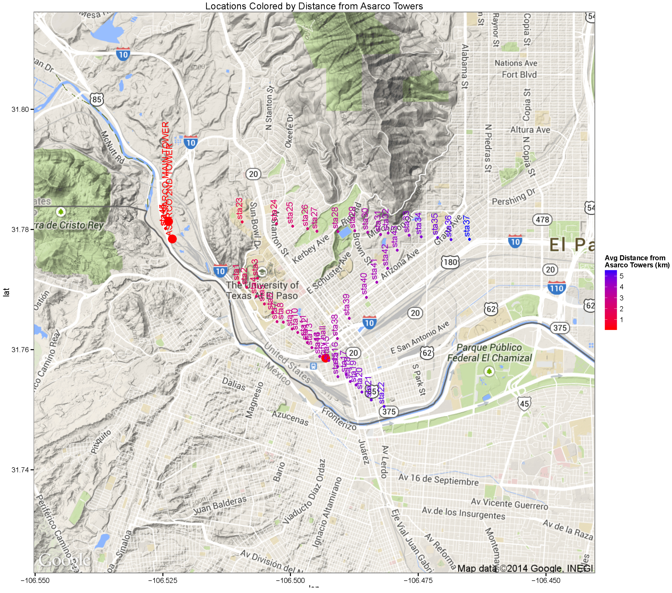
Figure 1 represents the map of the different recording locations throughout the area of El Paso. The color legend indicates their distances from the towers. In
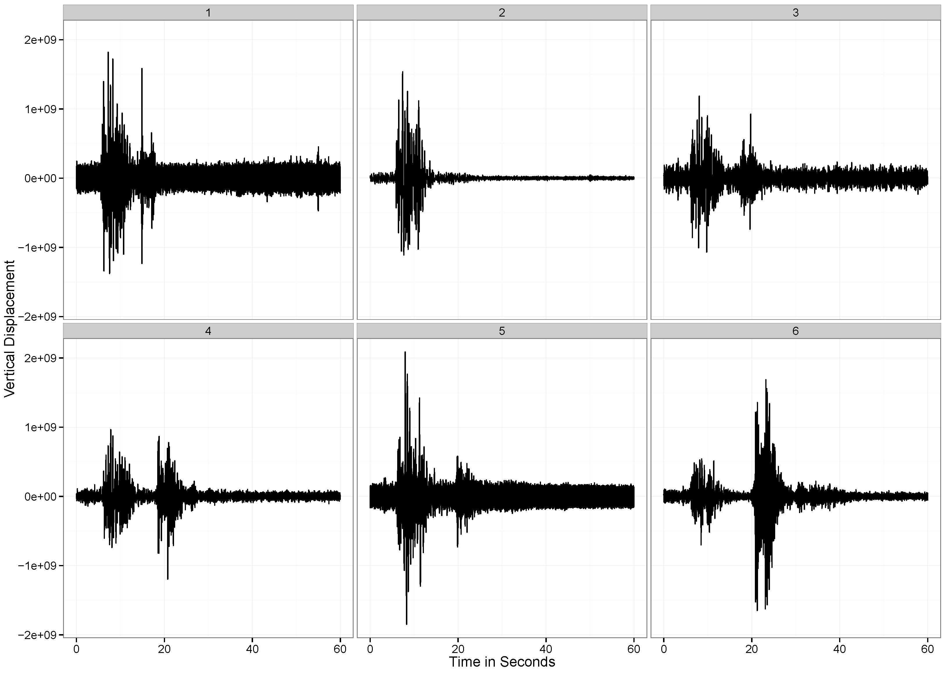
Figure 2, we observe the vertical displacement of the ground at each of the six stations that we are considering for the present analysis. As showed in all plots, there are two distinct periods of vibration in the ground. The first corresponds to the explosion, and the second corresponds to the time at which the detonated tower makes impact with the ground. The vertical displacements are listed graphically in
Figure 3.
Figure 1.
Location of the Measurement Stations Colored by Distance from the two detonation sites.
Figure 1.
Location of the Measurement Stations Colored by Distance from the two detonation sites.
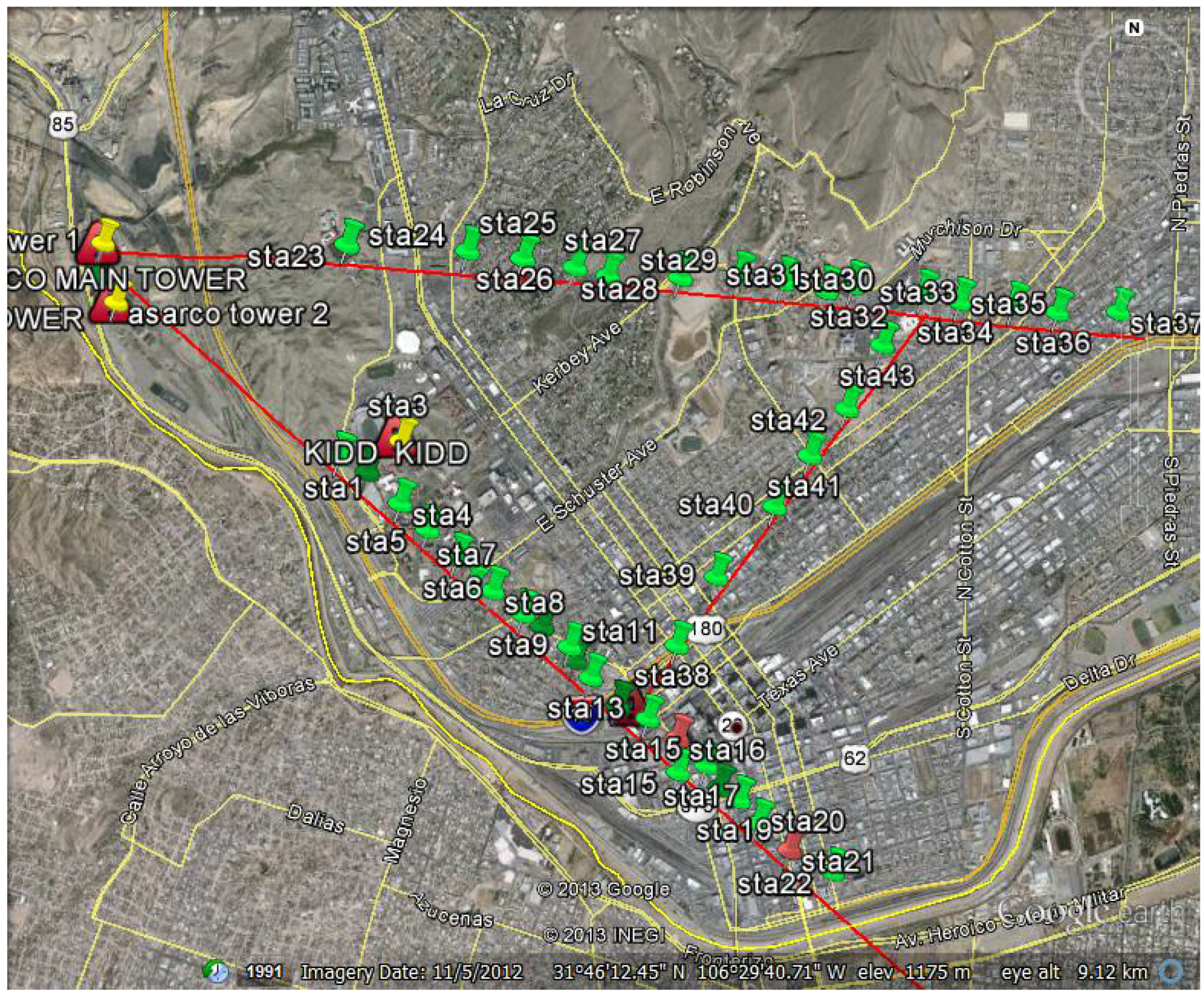
Figure 2.
The Project location map.
Figure 2.
The Project location map.
3. Spline Smoothing Methods
In numerical analysis, interpolation ([
5]) is a process for estimating values that lie within the range of a known discrete set of data points. In engineering and science, one often has a number of data points, obtained by sampling or experimentation, which represent the values of a function for a limited number of values of the independent variable. It is often required to interpolate (
i.e., estimate) the function at an intermediate value of the independent variable. This may be achieved by curve fitting or regression analysis.
Another similar problem is to approximate complicated functions by using simple functions. Suppose we know a formula to evaluate a function but its too complex to calculate at a given data point. A few known data points from the original function can be used to create an interpolation based on a simpler function. Of course, when a simple function is used to estimate data points from the original, interpolation errors are usually present; however, depending on the problem domain and the interpolation method that was used, the gain in simplicity may be of greater value than the resultant loss in accuracy. There is another kind of interpolation in mathematics called “Interpolation of operators". The error analysis of these methods can be found in [
6].
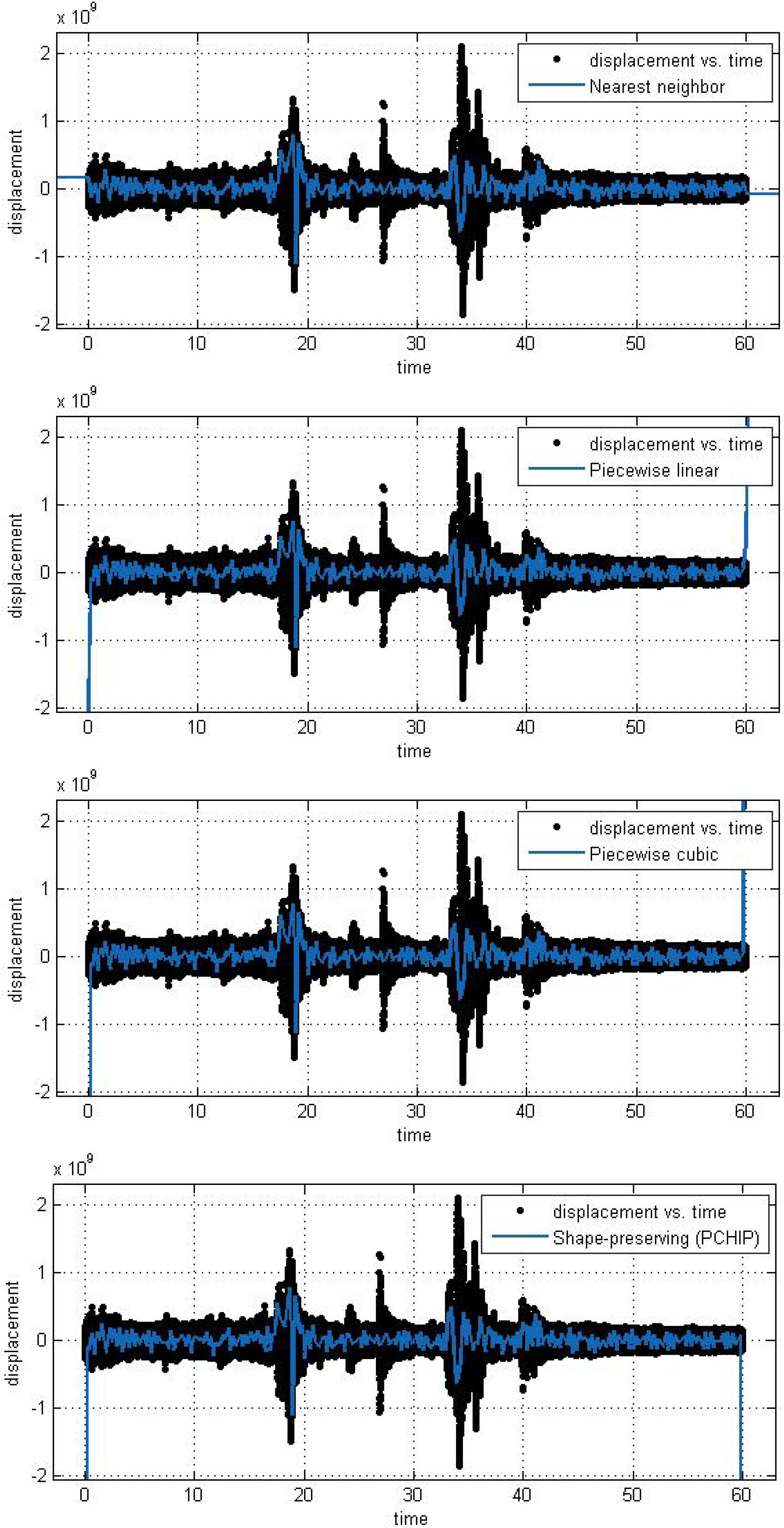
In this work, we have implemented four simple interpolation models to study the present data. Below we provide a brief description of the interpolation methods:
3.1. Nearest-Neighbor Interpolation
Nearest-neighbor interpolation (also known as proximal interpolation) is a simple method of multivariate interpolation in one or more dimensions. The nearest neighbor algorithm selects the value of the nearest point and does not consider the values of neighboring points at all, yielding a piecewise-constant interpolant. The algorithm is very simple to implement and is commonly used (usually along with mipmapping) in real-time 3D rendering to select color values for a textured surface.
The training examples are vectors in a multidimensional feature space, each one with a class label. The training phase of the algorithm consists only of storing the feature vectors and class labels of the training samples. In the classification phase, k is a user-defined constant, and an unlabeled vector (a query or test point) is classified by assigning the label which is most frequent among the k training samples nearest to that query point. A commonly used distance metric for continuous variables is the Euclidean distance. For discrete variables, such as for text classification, another metric can be used, such as the overlap metric (or Hamming distance). In the context of gene expression microarray data, for example, has also been employed with correlation coefficients such as Pearson and Spearman. Often, the classification accuracy of can be improved significantly if the distance metric is learned with specialized algorithms such as Large Margin Nearest Neighbor or Neighborhood components analysis. A drawback of the basic “majority voting" classification occurs when the class distribution is skewed. That is, examples of a more frequent class tend to dominate the prediction of the new example, because they tend to be common among the k nearest neighbors due to their large number. One way to overcome this problem is to weight the classification, taking into account the distance from the test point to each of its k nearest neighbors. The class (or value, in regression problems) of each of the k nearest points is multiplied by a weight proportional to the inverse of the distance from that point to the test point. Another way to overcome skew is by abstraction in data representation. For example in a self-organizing map (SOM), each node is a representative (a center) of a cluster of similar points, regardless of their density in the original training data. can then be applied to the SOM.
Figure 3.
The vertical displacement of the ground observed at the six measurement stations.
Figure 3.
The vertical displacement of the ground observed at the six measurement stations.
3.2. Bilinear Interpolation
Bilinear interpolation is a special technique which is an extension of regular linear interpolation for interpolation functions of two variables (i.e., x and y) on a regular 2D grid. The main idea is to perform linear interpolation first in one direction, and then again in the other direction. Although each step is linear in the sampled values and in the position, the interpolation as a whole is not linear but rather quadratic in the sample location. Bilinear interpolation is a continuous fast method where one needs to perform only two operations: one multiply and one divide; bounds are fixed at extremes.
3.2.1. Algorithm
Suppose that we want to find the value of the unknown function f at the point . It is assumed that we know the value of f at the four points and .
We first do linear interpolation in the
x-direction. This yields
where
,
where
.
We next proceed by interpolating in the
y-direction
This follows the desired estimate of
We note that the same result will be achieved by executing the y-interpolation first and x-interpolation second.
3.2.2. Unit Square
If we select the four points where
f is given to be
and
as the unit square vertices, then the interpolation formula simplifies to:
3.2.3. Nonlinear
Contrary to what the name suggests, the bilinear interpolant is not linear; nor is it the product of two linear functions. In other words, the interpolant can be written as
where
In both cases, the number of constants (four) correspond to the number of data points where f is given. The interpolant is linear along parallel lines to either the x or the y direction, equivalently if x or y is set constant. Along any other straight line, the interpolant is quadratic. However, even if the interpolation is not linear in the position (x and y), it is linear in the amplitude, as it is apparent from the equations above: all the coefficients , are proportional to the value of the function f.
The result of bilinear interpolation is independent of which axis is interpolated first and which second. If we had first performed the linear interpolation in the y-direction and then in the x-direction, the resulting approximation would be the same. The obvious extension of bilinear interpolation to three dimensions is called trilinear interpolation. This process needs no arithmetic operations and is very fast. It has discontinuities at each value and its bounds are fixed at extreme points.
3.3. Bicubic Interpolation
Bicubic interpolation [
7] is an extension of cubic interpolation for interpolating data points on a two dimensional regular grid. The interpolated surface is smoother than corresponding surfaces obtained by bilinear interpolation or nearest-neighbor interpolation. Bicubic interpolation can be accomplished by using either Lagrange polynomials, cubic splines, or cubic convolution algorithms.
Suppose the function values f and the derivatives
and
are known at the four corners
of the unit square. The interpolated surface can then be written
The interpolation problem consists of determining the 16 coefficients
. Matching
with the function values yields four equations,
All the directional coefficients can be determined by the following identities:
This procedure yields a surface on the unit square which is continuous and with continuous derivatives. Bicubic interpolation on an arbitrarily sized regular grid can then be accomplished by patching together such bicubic surfaces, ensuring that the derivatives match on the boundaries. If the derivatives are unknown, they are typically approximated from the function values at points neighbouring the corners of the unit square, e.g., by using finite differences. The unknowns in the coefficients can be easily determined by solving a linear equation.
3.4. Shape-Preserving (PCHIP)
In numerical analysis, a cubic Hermite spline or cubic Hermite interpolator is a spline where each piece is a third-degree polynomial specified in Hermite form, that is, by its values and first derivatives at the end points of the corresponding domain interval. Cubic Hermite splines are typically used for interpolation of numeric data specified at given argument values , to obtain a smooth continuous function. The data should consist of the desired function value and derivative at each . (If only the values are provided, the derivatives must be estimated from them.) The Hermite formula is applied to each interval () separately. The resulting spline will be continuous and will have continuous first derivative. Cubic polynomial splines can be specified in other ways, the Bézier form being the most common. However, these two methods provide the same set of splines, and data can be easily converted between the Bézier and Hermite forms; so the names are often used as if they were synonymous. Cubic polynomial splines are extensively used in computer graphics and geometric modeling to obtain curves or motion trajectories that pass through specified points of the plane or three-dimensional space. In these applications, each coordinate of the plane or space is separately interpolated by a cubic spline function of a separate parameter t. Cubic splines can be extended to functions of two or more parameters, in several ways. Bicubic splines (Bicubic interpolation) are often used to interpolate data on a regular rectangular grid, such as pixel values in a digital image or altitude data on a terrain. Bicubic surface patches, defined by three bicubic splines, are an essential tool in computer graphics. Piecewise cubic Hermite interpolation are also known as Shape-preserving interpolation technique. This method preserves monotonicity and the shape of the data.
Interpolation on a Single Interval
4. Statistical Analysis of Variability
We have used a number of interpolation methods to interpolate the movement of the displacement curve over time. Another aspect of the data we study here is the local variability of this displacement.
Note that the raw observations are the vertical displacements of the ground measured every millisecond. This measure takes both positive and negative values. In the ambient state (when the ground is not subjected to any deviations), there is some (though subdued) deviation in the ground. For example, in
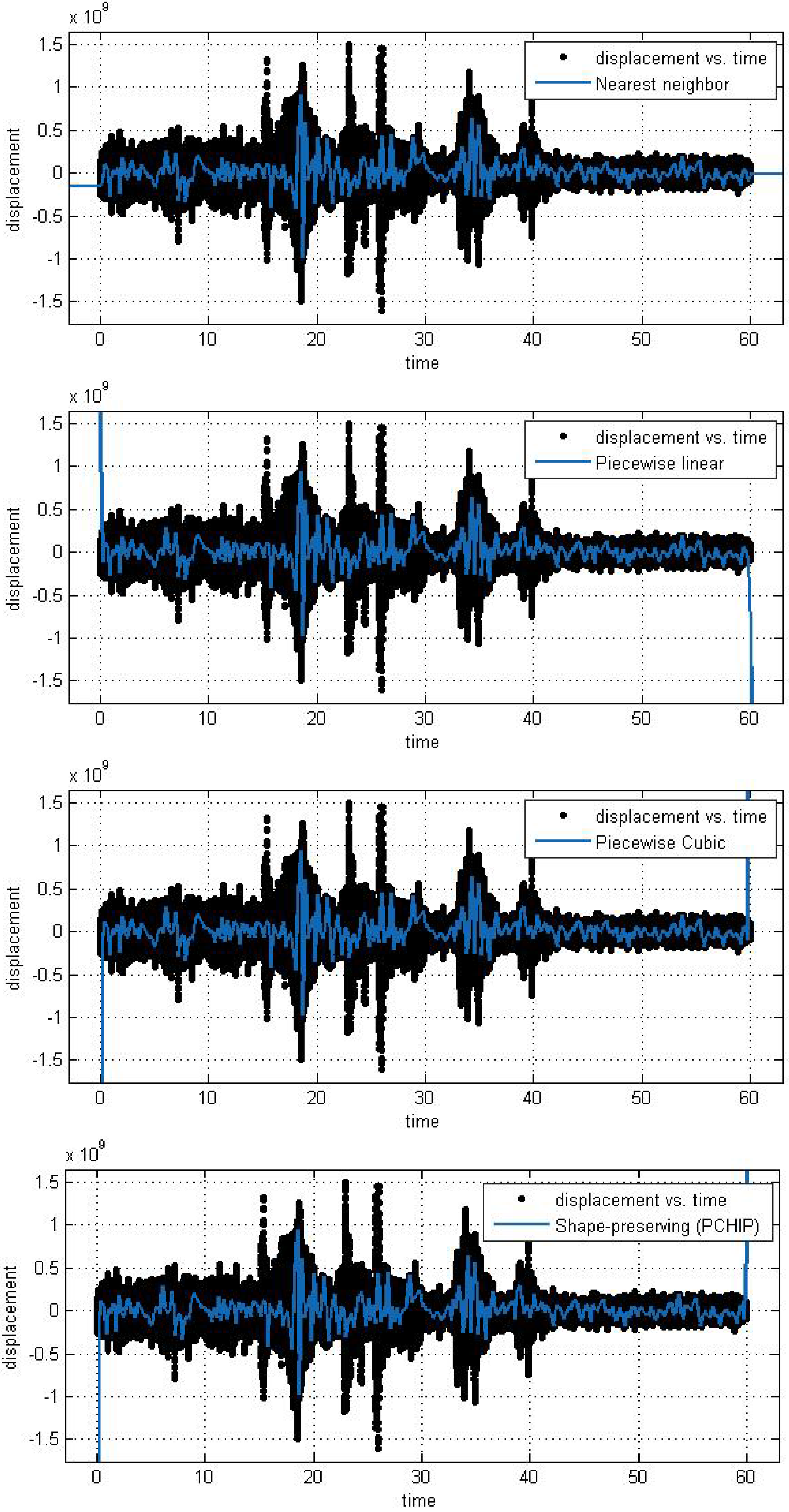
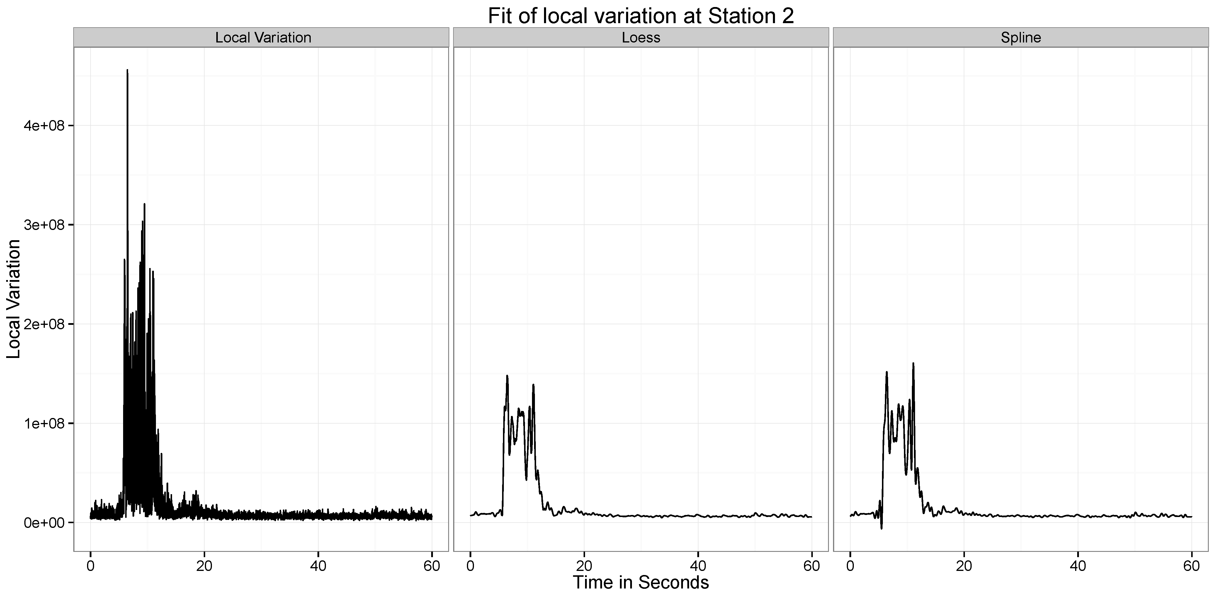
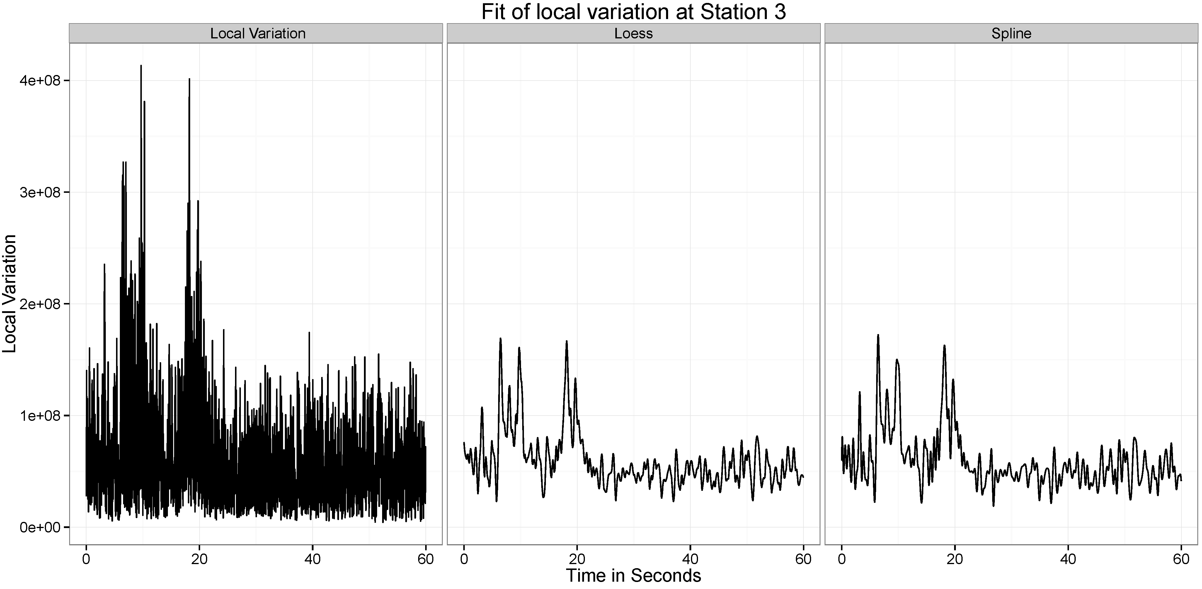
Figure 2, we see that after 30 seconds, at station 3, there is considerable local variation. However, at station 2, this local variation is much lower. This can be an effect of the differences in the quality of the ground (hard soil versus soft soil) at these two locations.
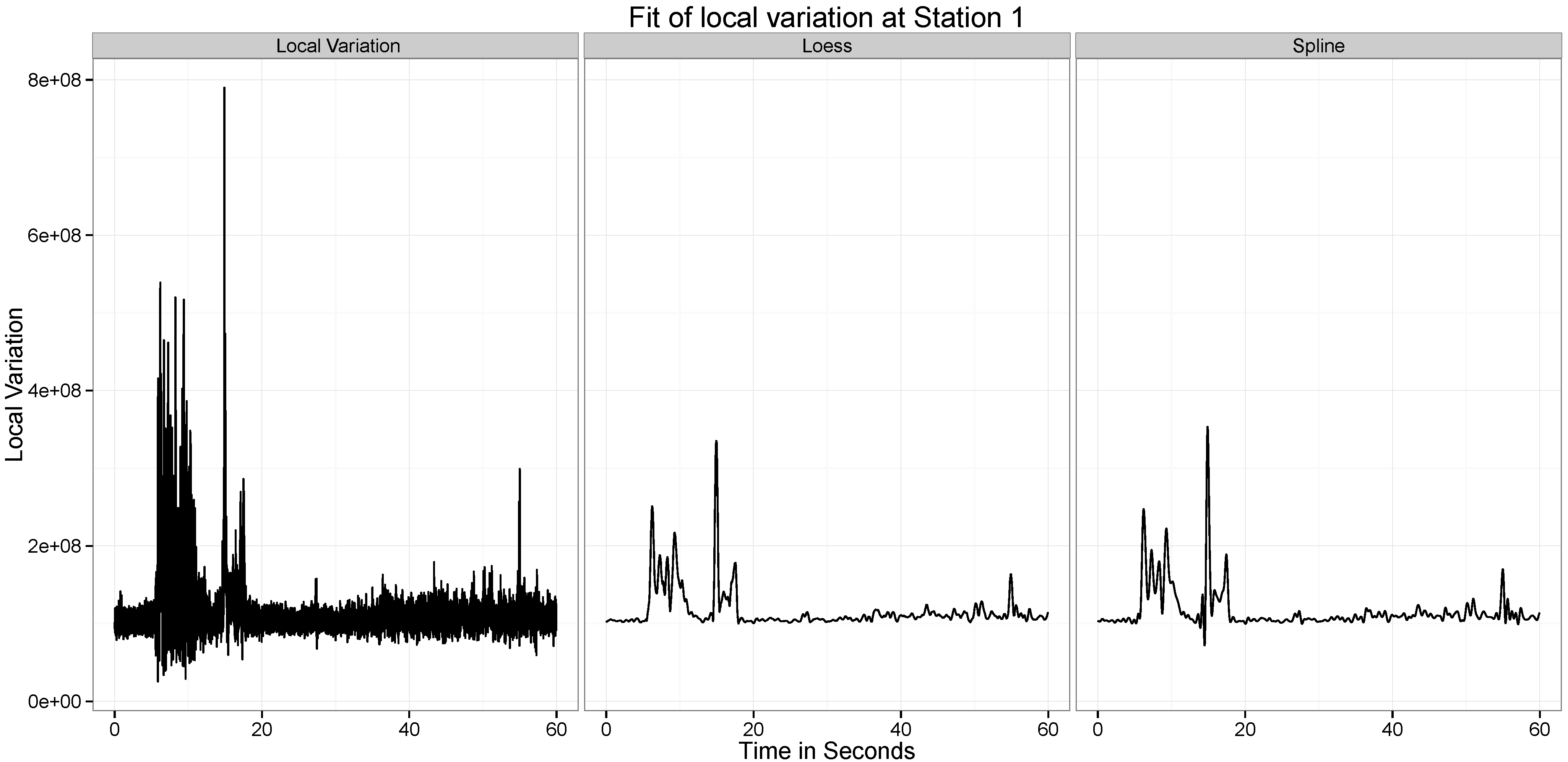
However, an important thing to note is how the local variation increases when the wave passes through a particular location. For instance, at around 10 seconds, at Station 1, the ground experiences a spike in the variability in the position of the ground. To capture the local variability of the time series, we define the following measure.
where
.
is the standard deviation of
k terms starting from the
observation.
After computation of this filter on the series, we next fit two statistical smoothing methods to these two series. We apply the Loess smoothing method (with local polynomials of degree 2) and the Smoothing Spline.
4.1. Loess Smoothing
Lowess and Loess (locally weighted scatterplot smoothing) are two strongly related non-parametric regression methods that include multiple regression models in a
k-nearest-based meta model [
8].“Loess” is a generic version of “Lowess”, its name arises in “LOcal regrESSion”. The two methods arise on the linear and nonlinear least square regression. These methods are more powerful and effective for studies in which the classical regression procedures cannot produce satisfactory results or cannot be efficiently applied without undue labor. Loess incorporates much of the simplicity of the linear least squares regression with some room for nonlinear regression. It works by fitting simple models to localized data subsets in order to construct a function that describes pointwise the deterministic part associated to the variation of data. The main advantage of this process is that it does not need to analyze data in order to determine a global function in order to fit a model to the entire data set, but only to a segment of data.
This method involves a lot of increased computation as it is a computationally intense procedure. However, in the modern computational set up, Lowess/Loess has been designed to take advantage of the current computational ability in order to achieve the goals that cannot be easily achieved by using traditional methods.
A smooth curve through a set of data points obtained by using an statistical technique is called a
Loess curve, particularly when the smoothed value is obtained by a weighted quadratic least squares regression over the span of values of the y-axis scattergram criterion variable. Similarly, the same process is called
Lowess curve when each smoothed value is given by weighted linear least squares regression over the span. Although some literature consider
Lowess and
Loess as synonymous, some key features of the local regression models are:
Definition of a Lowess/Loess model: Lowess/Loess, originally proposed by Cleveland and further improved by Cleveland and Devlin [
9], specifically denoted a method that is also known as locally weighted polynomial regression. At each point in the data set a low-degree polynomial is fitted to a subset of the data, with explanatory variable values near the point whose response is being estimated. Weighted least square method is implemented in order to fit the polynomial where more weightage is given to points near the point whose response is being estimated and less weightage to points further away. The value of the regression function at the point is then evaluated by calculating the local polynomial by using the explanatory variable values for that data point. One needs to compute the regression function values for each of the
n data points in order to complete the Lowess/Loess process. Many details in this method, such as degree of the polynomial model and weights, are flexible.
Local subsets of data: The subset of data used for each weighted least square fit in Lowess/Loess is decided by a nearest neighbors algorithm. One can predetermine the specific input to the process called the “bandwidth" or “smoothing parameter", it determines how much of the data is used to fit each local polynomial according to its needs. The smoothing parameter α, takes values between and 1, with λ denoting the degree of the local polynomial, the value of α is the proportion of data used in each fit. The subset of data used in each weighted least squares fit comprises the points (rounded to the next larger integer) whose explanatory variable values are closest to the point at which the response is being evaluated. The smoothing parameter α is named because it controls the flexibility of the Lowess/Loess regression function. Large values of α produce the smoothest functions that wiggle the least in response to fluctuations in the data. The smaller α is, the closer the regression function will conform to the data, but using a very small value for the smoothing parameter is not desirable since the regression function will eventually start to capture the random error in the data. For the majority of the Lowess/Loess applications, α values are chosen in the interval.
Degree of local polynomials: First and second degree polynomial are used to fit local polynomials to each subset of data. That means, either a locally linear or quadratic function are most useful; using a zero polynomial turns Lowess/Loess into a weighted moving average. Such a simple model might work well for some situations, and may approximate the underlying function well enough. Higher-degree polynomial methods perform very good in theory although this method doesn't agree with the spirit of Lowess/Loess method: Lowess/Loess is based on the idea that any function can be approximated in a small neighborhood by a low-degree polynomial and simple models can be easily fitted to data. High-degree polynomials would tend to overfit the data in each subset and are numerically unstable, making precise calculation almost impossible.
Weight function: The weight function assigns more weight to the data points nearest the point of evaluation and less weight to the data points that are further away. The idea behind this method is that the points near each other in the explanatory variable space are more likely to be associated to each other in a simple way than the points that are located further away. Following this argument, points that are likely to follow the local model best influence the local parameter estimate the most. Points that are less likely to actually conform to the local model have less influence on the local model parameter estimation. The Lowess/Loess methods use the traditional tri-cubed weight function. However, any other weight function that satisfies the properties that are presented in [
10] could also be taken into consideration. The process of calculating the weight for a specific point in any localized subset of data is done by evaluating the weight function at the distance between the point and the point of estimation, after scaling the distance so that the maximum absolute distance over all possible points in the subset of data is exactly one.
Advantages and Disadvantages of Lowess/Loess: As mentioned above, the biggest advantage of the Lowess/Loess methods over many other methods is the fact that they do not require the specification of a function to fit a model over the global sample data. Instead, an analyst has to provide a smoothing parameter value and the degree of the local polynomial. Moreover, the flexibility of this process makes it very appropriate for modeling complex processes for which no theoretical model exists. The simplicity for executing the methods, make these processes very popular among the modern era regression methods that fit the general framework of least squares regression, but having a complex deterministic structure. Although they are less obvious than some of the other methods related to linear least squares regression, Lowess/Loess also enjoy most of the benefits generally shared by the other methods, the most important of those is the theory for computing uncertainties for prediction, estimation and calibration. Many other tests and processes used for validation of least square models can also be extended to Lowess/Loess.
The major drawback of Lowess/Loess is the inefficient use of data compared to other least square methods. Typically it requires fairly large, densely sampled data sets in order to create good models, the reason behind is that the Lowess/Loess methods rely on the local data structure when performing the local fitting, thus proving less complex data analysis in exchange of increased computational cost. The Lowess/Loess methods do not produce a regression function that is represented by a mathematical formula, what may be a disadvantage: It can make it very difficult to transfer the results of the numerical analysis to other researchers, in order to transfer the regression function to others, they would need the data set and the code for Lowess/Loess calculations. In non-linear regression, on the other hand, it is only necessary to write down a functional form in order to provide estimates of the unknown parameters and the estimated uncertainty. In particular, the simple form of Lowess/Loess can not be applied to mechanistic modeling where the fitted parameters specify particular physical properties of the system. It is worth mentioning the computation cost associated with this procedure, although this should not be a problem in the modern computing environment, unless the data sets being used are very large. Lowess/Loess also have a tendency to be affected by the outliers in the data set, like any other least square methods. There is an iterative robust version of Lowess/Loess (see [
10]) that can be applied to reduce sensitivity to outliers, but if there exist too many extreme outliers, this robust version also fails to produce the desired results.
4.2. Smoothing Spline
The smoothing spline is a smoothing approach where the complexity of the fit is controlled by regularization. The goal of this approach is to, among all continuous functions
with two continuous derivatives, find the one that minimizes the penalized residual sum of squares [
11].
where
λ is a fixed smoothing parameter. The first term measures the closeness to the data, while the second term penalizes the curvature of the function. While the above equation is defined on an infinite dimensional space, it can be reduced to a fairly simple optimization routine. The above formula can be seen to lead to the following estimate
where
,
and
. Also,
are an N-dimensional set of basis functions for representing this family of natural splines. There are efficient computational techniques for smoothing splines. More details can be found in [
11,
12]. A smoothing spline with prechosen
λ is an example of a linear smoother (as in linear operator), as below
Then, the effective degrees of freedom may be defined as . In our exercise, we found that the value of degrees of freedom of 200 lead to good quality fits of the data, capturing the structure of the underlying series.
5. Results and Discussions
In this section we present the numerical findings of the mathematical and statistical models that are the focus of this study.
5.1. Mathematical Models Applied to the Time Series
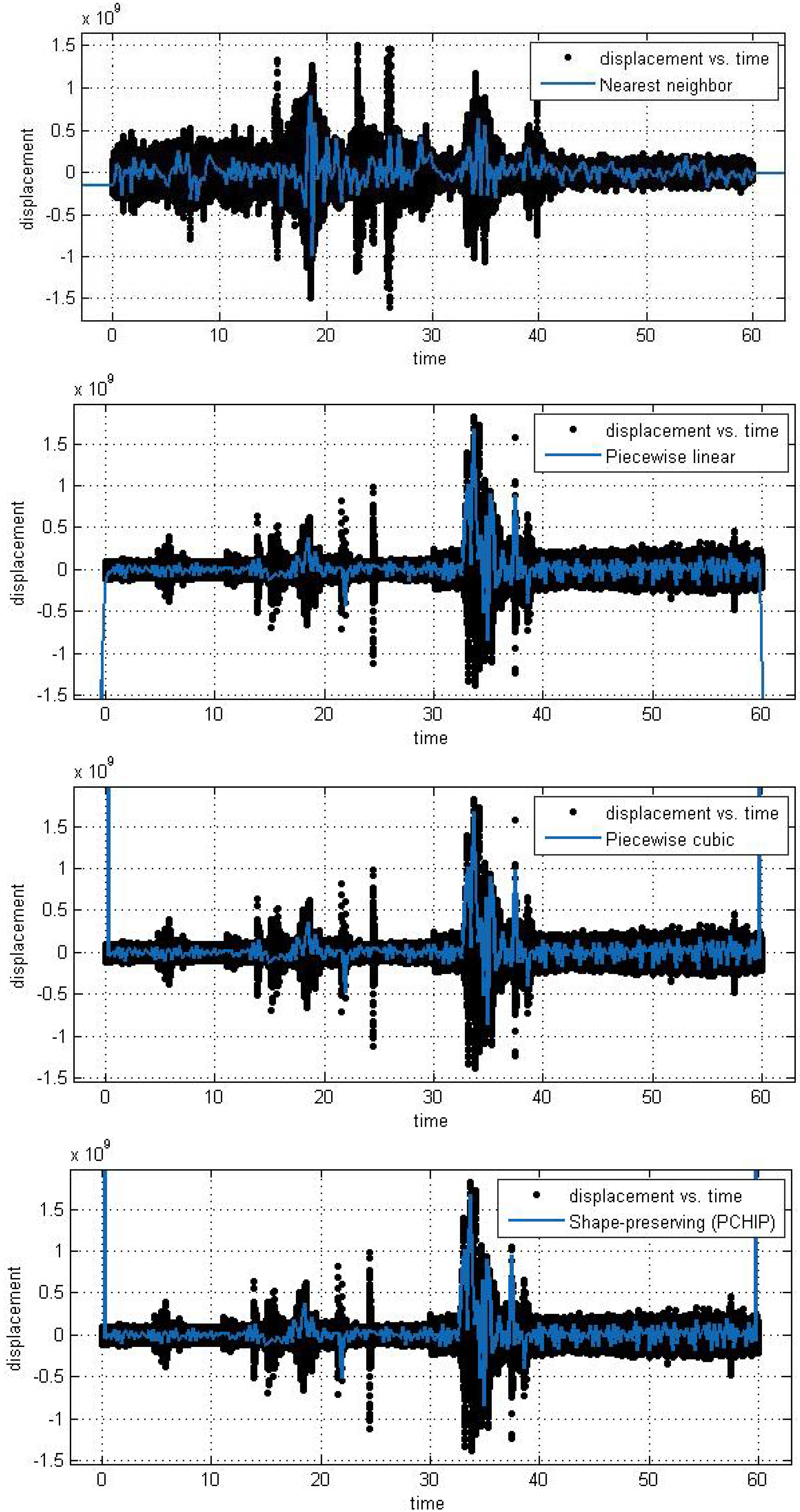
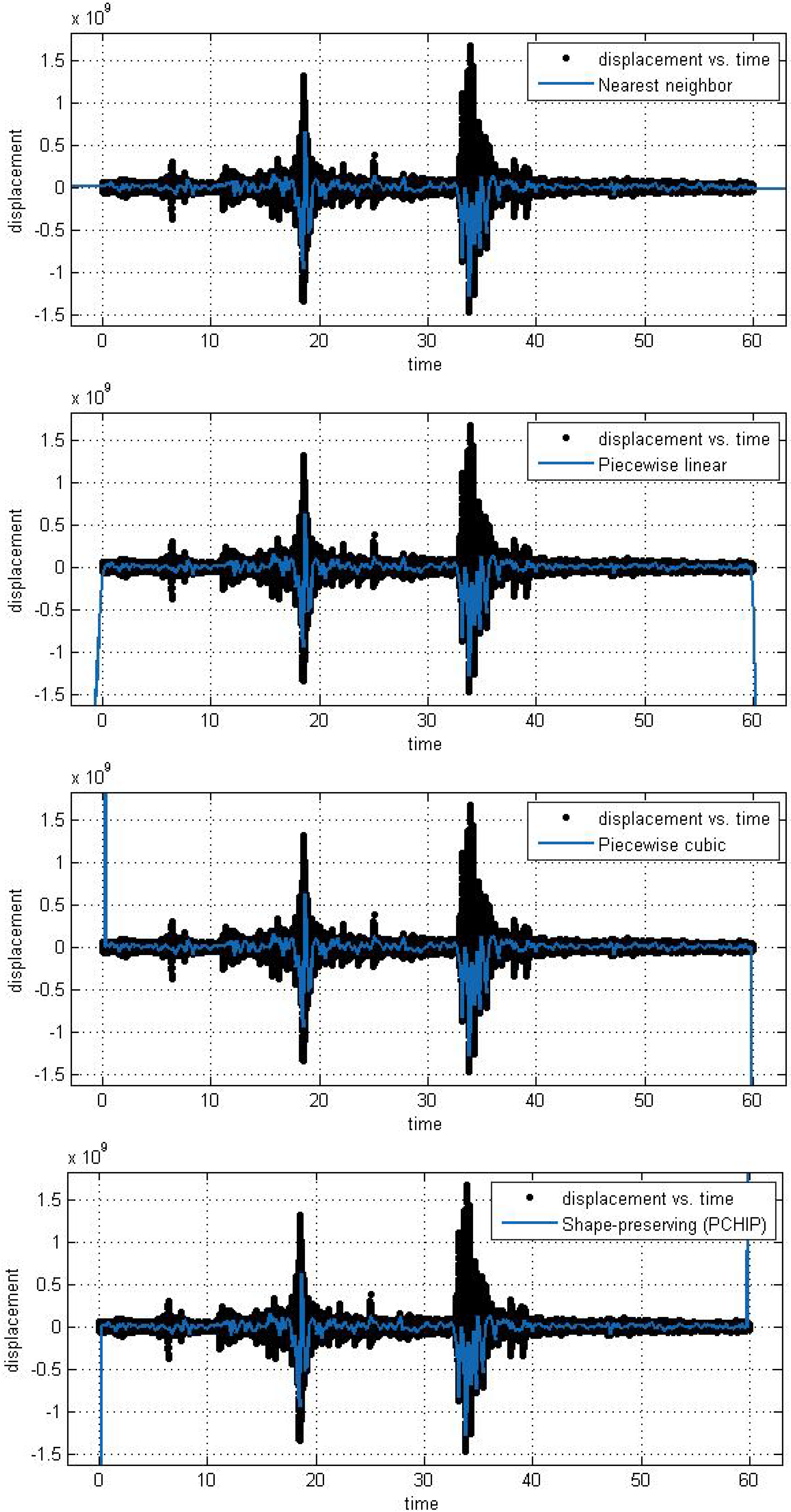
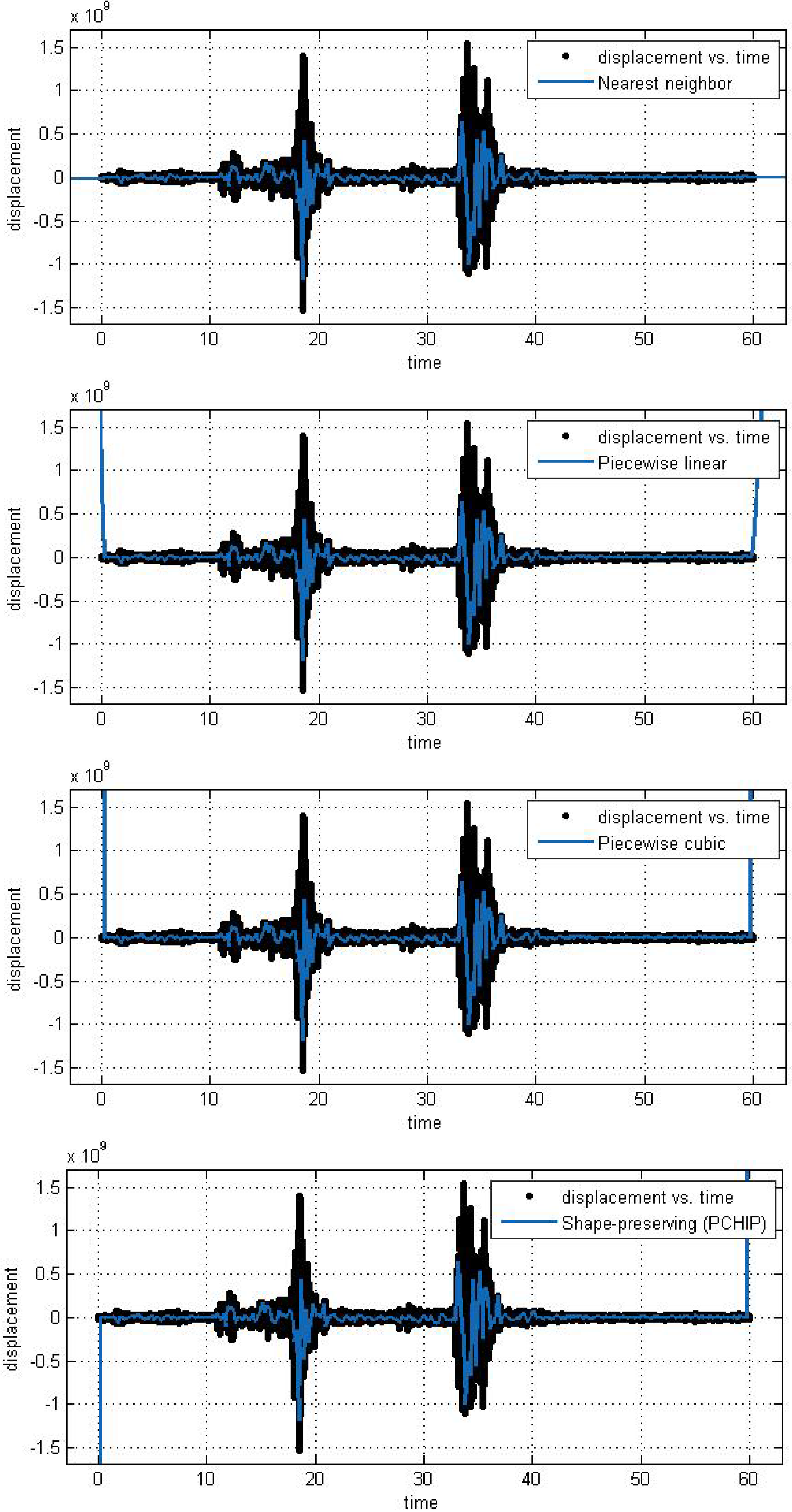
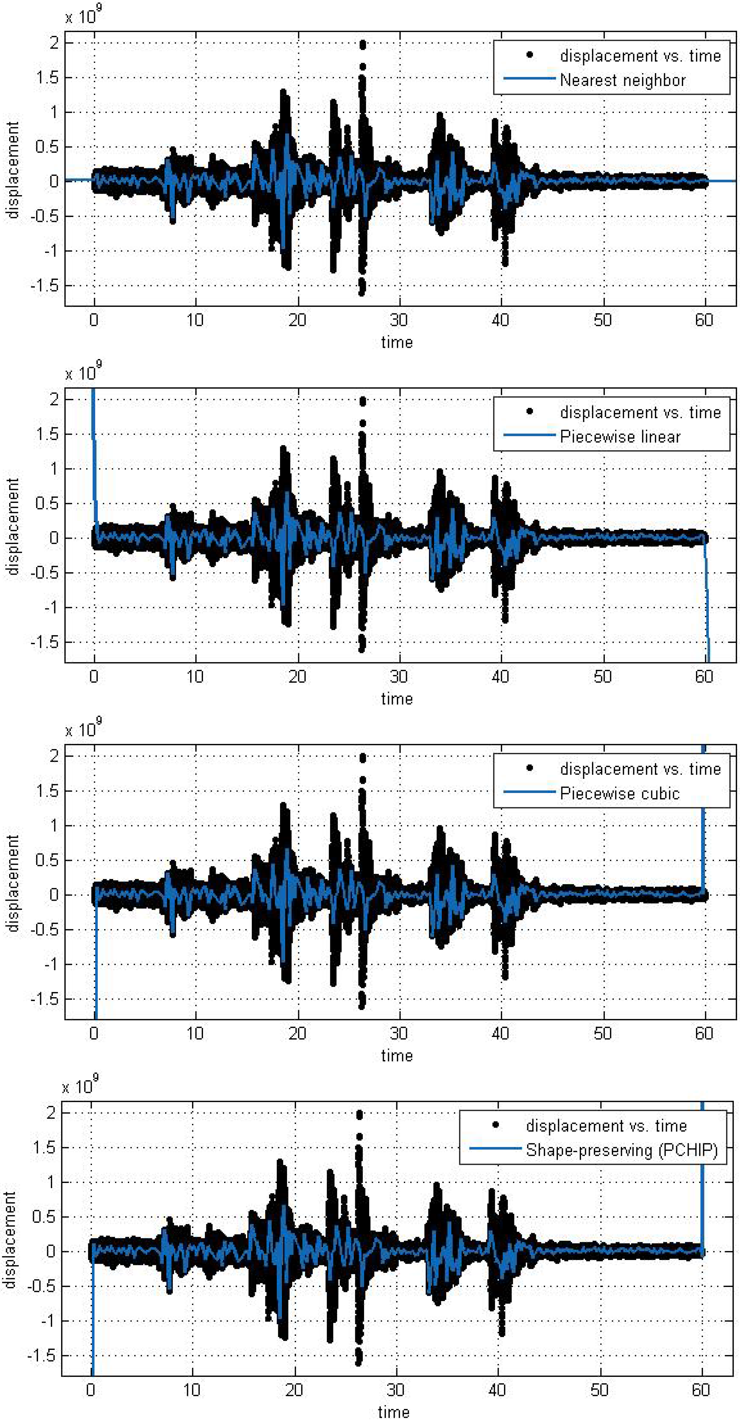
In this subsection, we analyze the efficiency and accuracy of the different spline interpolation techniques that were applied to the Asarco demolition seismic data set. In the first numerical exploration, we applied four different interpolation techniques to the data recorded at six randomly selected stations. The numerical analysis was performed using the curve fitting toolbox in Matlab in order to generate the interpolation results. Results are presented for six randomly selected stations where the displacement of the ground through a seismograph are available. The different modeling techniques performed equally good. According to these results, spline interpolation models are adequate for the analysis of this class of time series data and may open a new approach for studying the seismic time series data. All our numerical findings in application of the Spline interpolants are shown in
Figure 4,
Figure 5,
Figure 6,
Figure 7,
Figure 8 and
Figure 9.
Figure 4.
Different interpolant curve fitted on the data from Station 1.
Figure 4.
Different interpolant curve fitted on the data from Station 1.
Figure 5.
Different interpolant curve fitted on the data from Station 2.
Figure 5.
Different interpolant curve fitted on the data from Station 2.
Figure 6.
Different interpolant curve fitted on the data from Station 3.
Figure 6.
Different interpolant curve fitted on the data from Station 3.
Figure 7.
Different interpolant curve fitted on the data from Station 4.
Figure 7.
Different interpolant curve fitted on the data from Station 4.
Figure 8.
Different interpolant curve fitted on the data from Station 5.
Figure 8.
Different interpolant curve fitted on the data from Station 5.
Figure 9.
Different interpolant curve fitted on the data from Station 6.
Figure 9.
Different interpolant curve fitted on the data from Station 6.
5.2. Statistical Analysis of Local Variation in Time Series
Figure 10,
Figure 11,
Figure 12,
Figure 13,
Figure 14 and
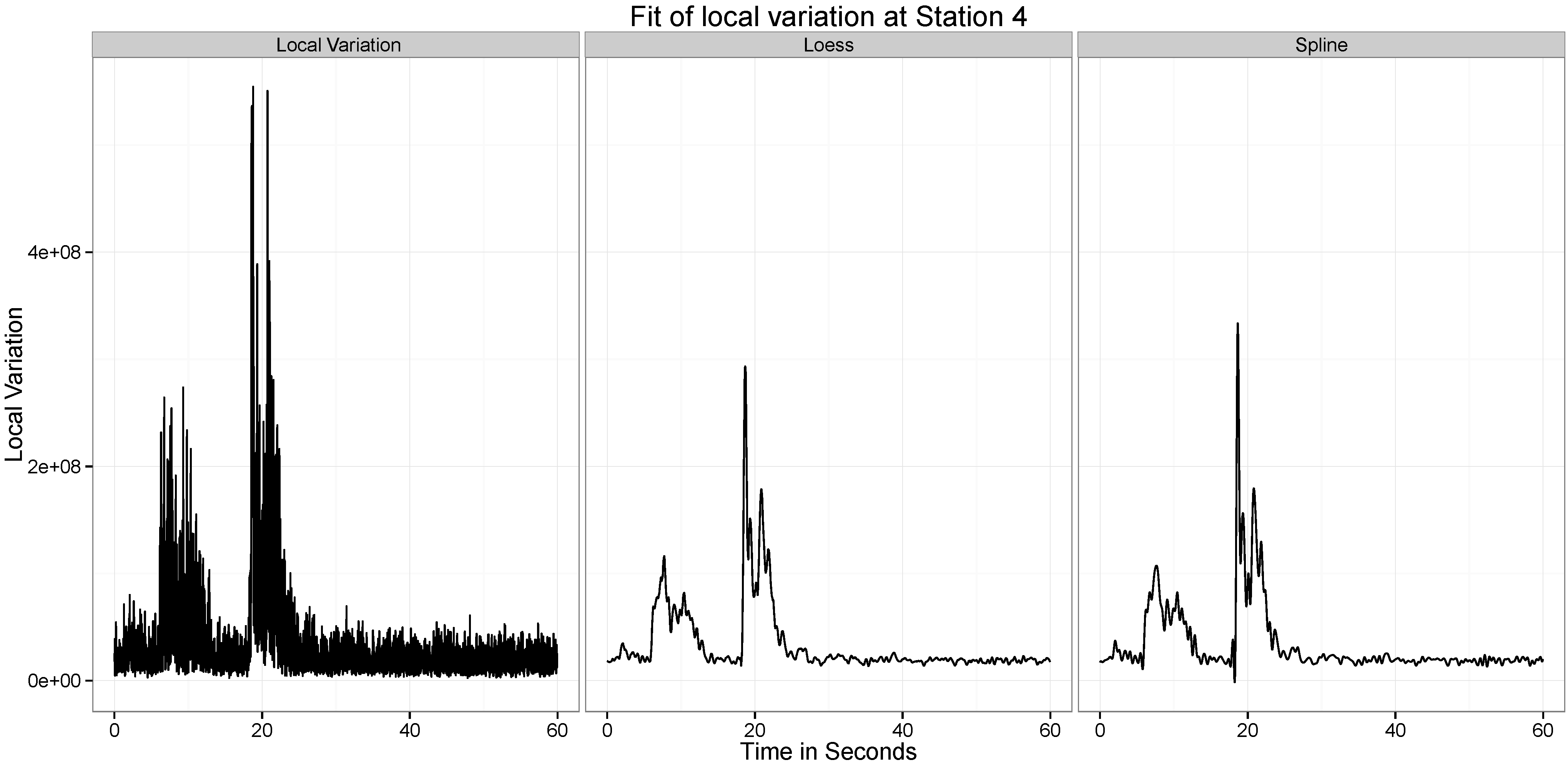
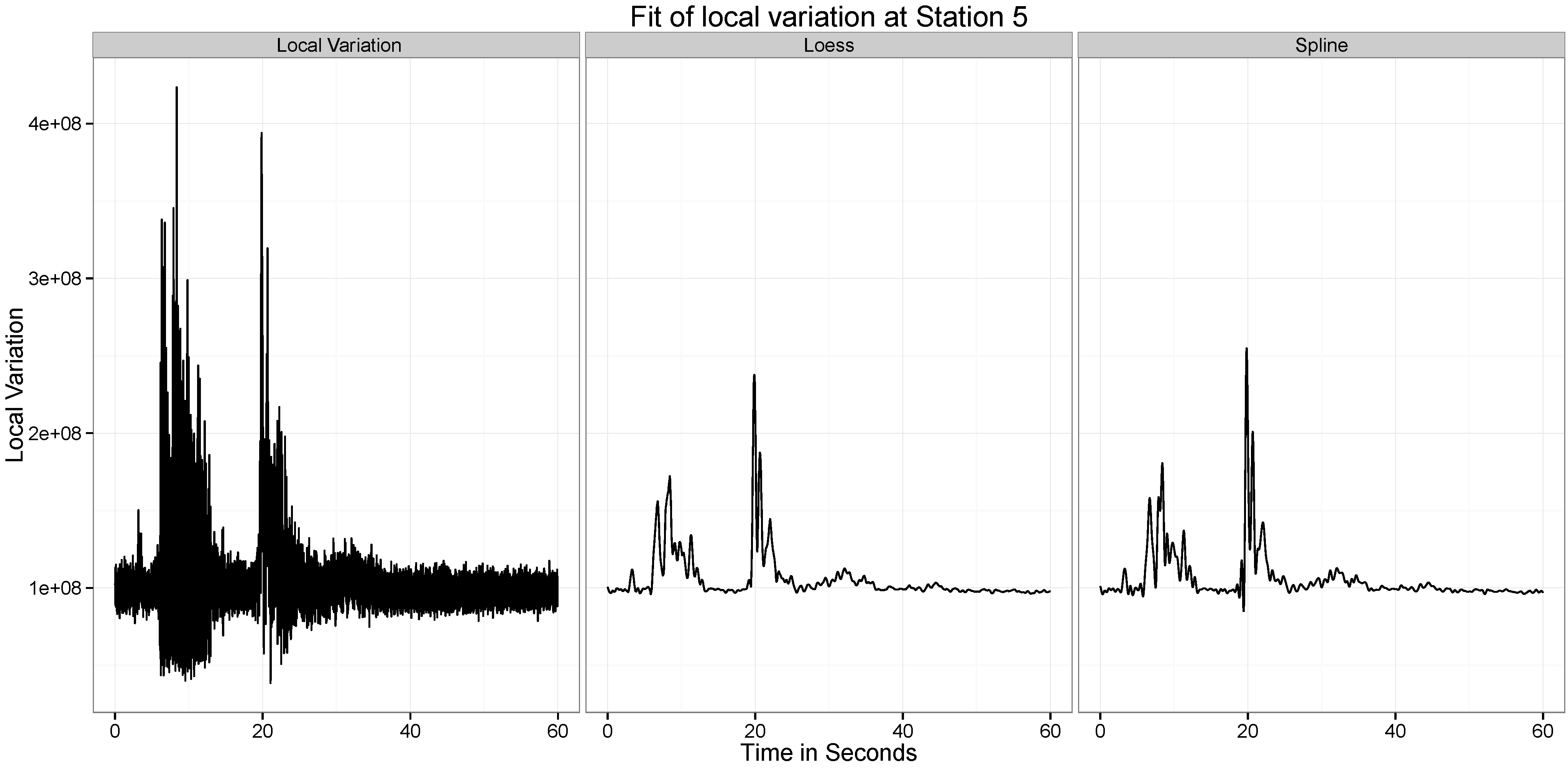
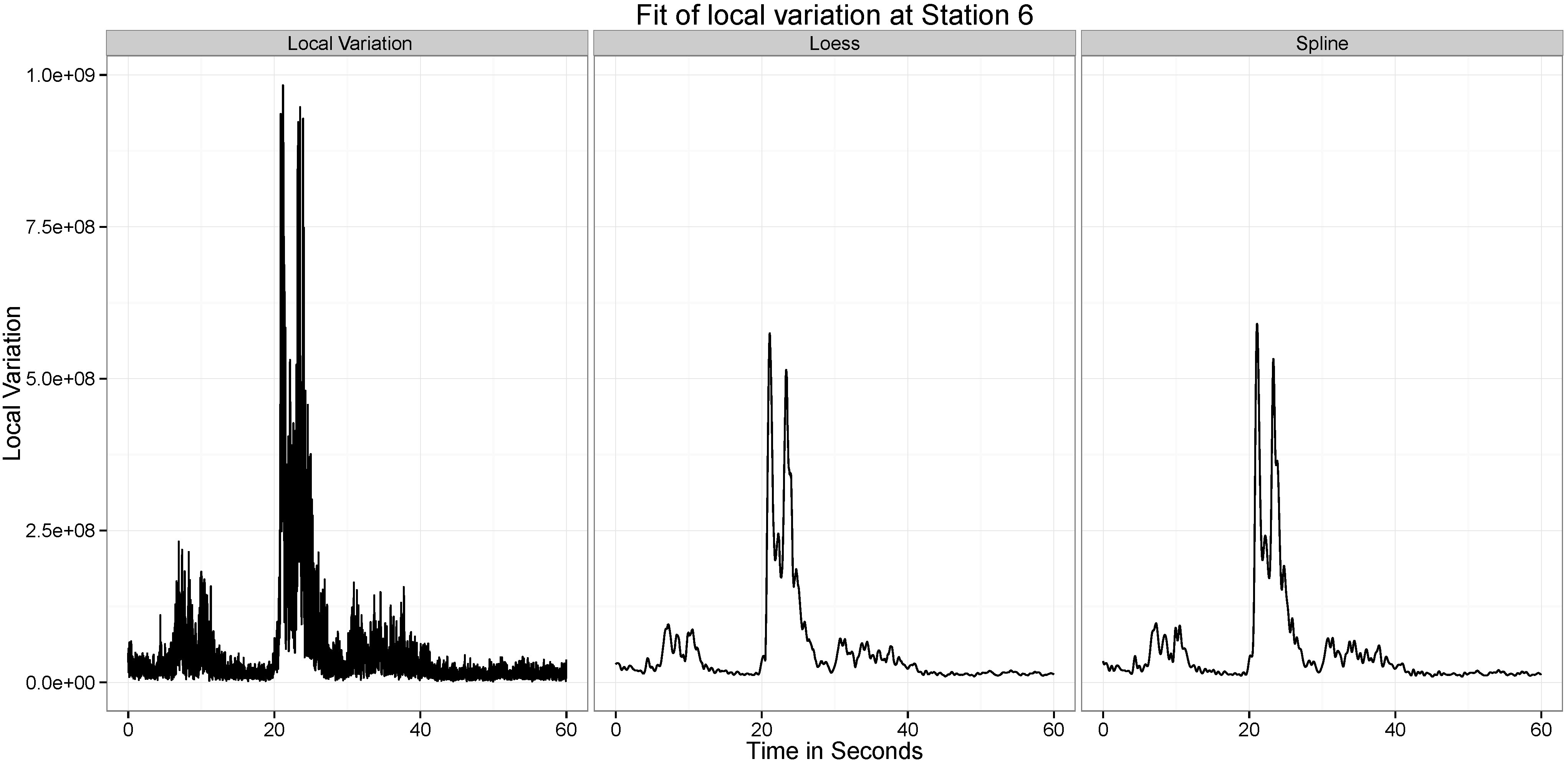
Figure 15 present our analysis of the local variation in the time series. In the first line plot of each image is the local standard deviation (
) of the series at that time point. As can be seen from all the images, the local variations are stable when there is no wave at the location at the time point, but when the wave passes the location, the local variation curve experiences significant vibrations.
There are two distinct spikes in the variability of the curve, the first corresponds to when the explosion happens. The second corresponds to when the tower hits the ground. Both of these apparent at Stations and 6. At Station 2 the effect of the second wave is not observed.
The two statistical approaches evaluated to test this ability to provide a summary of this variation are the Smoothing Spline and the Loess Smoothing approaches. For example, as can be seen from
Figure 11, the two explosions are well captured by both approaches. Across all the different datasets, the performance of the two approaches are similar, though the spline approach seems to be capturing a little more of the variability.
Figure 10.
Location of the Measurement Stations Colored by Distance from the two detonation sites.
Figure 10.
Location of the Measurement Stations Colored by Distance from the two detonation sites.
Figure 11.
Location of the Measurement Stations Colored by Distance from the two detonation sites.
Figure 11.
Location of the Measurement Stations Colored by Distance from the two detonation sites.
Figure 12.
Location of the Measurement Stations Colored by Distance from the two detonation sites.
Figure 12.
Location of the Measurement Stations Colored by Distance from the two detonation sites.
Figure 13.
Location of the Measurement Stations Colored by Distance from the two detonation sites.
Figure 13.
Location of the Measurement Stations Colored by Distance from the two detonation sites.
Figure 14.
Location of the Measurement Stations Colored by Distance from the two detonation sites.
Figure 14.
Location of the Measurement Stations Colored by Distance from the two detonation sites.
Figure 15.
Location of the Measurement Stations Colored by Distance from the two detonation sites.
Figure 15.
Location of the Measurement Stations Colored by Distance from the two detonation sites.
6. Conclusions
In this paper, we have explored different mathematical and statistical interpolation techniques in their ability to properly capture the structure of seismometric time series. We have tested four mathematical interpolation methods and two statistical curve fitting approaches. We have fit these approaches to six different time series. These series do not have cyclical or trend in them, thus our approaches are more preferable here to traditional time series approaches like ARMIA and Exponential Smoothing approaches. While we do not directly compare the mathematical and statistical approaches on the same data, we see the obvious advantages of both approaches for seiemometric data arising on the Asarco demolitions.
Acknowledgments
The authors would like to thank and acknowledge Wikipedia for reference purposes.
Author Contributions
Kanadpriya Basu and Maria C. Mariani conceived and implemented the numerical methods, and wrote the paper; Laura Serpa provided the analyzed data and Ritwik Sinha performed the statistical analysis.
Conflicts of Interest
Authors declare that there are no conflict of interest.
References
- Mariani, M.C.; Florescu, I.; Sengupta, I.; Beccar Varela, M.P.; Bezdek, P.; Serpa, L. Lévy models and scale invariance properties applied to Geophysics. Phys. A Stat. Mech. Appl. 2013, 392, 824–839. [Google Scholar] [CrossRef]
- Habtemicael, S.; SenGupta, I. Ornstein-Uhlenbeck processes for geophysical data analysis. Phys. A Stat. Mech. Appl. 2014, 399, 147–156. [Google Scholar] [CrossRef]
- Mariani, M.C.; Basu, K. Local regression type methods applied to the study of geophysics and high frequency financial data. Phys. A Statist. Mech. Appl. 2014, 410, 609–622. [Google Scholar] [CrossRef]
- Mariani, M.C.; Basu, K. Spline interpolation techniques applied to the study of geophysical data. Phys. A Stat. Mech. Appl. 2015. [Google Scholar] [CrossRef]
- Philips, G. Interpolation and Approximation by Polynomials; Springer-Verlag: New York, NY, USA, 2003. [Google Scholar]
- Meng, T.; Geng, H. Error Analysis of Rational Interpolating Spline. Int. J. Math. Anal. 2011, 5, 1287–1294. [Google Scholar]
- Peisker, P. A Multilevel Algorithm for the Biharmonic Problem. Numer. Math. 1985, 46, 623–634. [Google Scholar] [CrossRef]
- Cleveland, W.S.; Grosse, E.; Shyu, W.M. Local regression models. In Statistical Models in S; Wadsworth and Brooks/Cole: Pacific Grove, CA, USA, 1992; pp. 309–376. [Google Scholar]
- Cleveland, W.S.; Devlin, S.J. Locally Weighted Regression: An Approach to Regression Analysis by Local Fitting. J. Am. Stat. Assoc. 1988, 83, 596–610. [Google Scholar] [CrossRef]
- Cleveland, W.S. Robust Locally Weighted Regression and Smoothing Scatterplots. J. Am. Stat. Assoc. 1979, 74, 829–836. [Google Scholar] [CrossRef]
- Hastie, T.; Friedman, J.; Tibshirani, R. The Elements of Statistical Learning, 2nd ed.; Springer-Verlag: New York, NY, USA, 2009. [Google Scholar]
- Green, P.J.; Silverman, B.W. Nonparametric Regression and Generalized Linear Models: A Rough. Penal. Approach; CRC Press: Boca Raton, FL, USA, 1993. [Google Scholar]
© 2015 by the authors; licensee MDPI, Basel, Switzerland. This article is an open access article distributed under the terms and conditions of the Creative Commons Attribution license (http://creativecommons.org/licenses/by/4.0/).


