New Iterative Methods for Solving Nonlinear Problems with One and Several Unknowns

Abstract

In this manuscript, a new type of study regarding the iterative methods for solving nonlinear models is presented. The goal of this work is to design a new fourth-order optimal family of two-step iterative schemes, with the flexibility through weight function/s or free parameter/s at both substeps, as well as small residual errors and asymptotic error constants. In addition, we generalize these schemes to nonlinear systems preserving the order of convergence. Regarding the applicability of the proposed techniques, we choose some real-world problems, namely chemical fractional conversion and the trajectory of an electron in the air gap between two parallel plates, in order to study the multi-factor effect, fractional conversion of species in a chemical reactor, Hammerstein integral equation, and a boundary value problem. Moreover, we find that our proposed schemes run better than or equal to the existing ones in the literature.

1. Introduction

The role of iterative methods in solving nonlinear problems of many branches of science and engineering has increased dramatically in recent years. One of the most important reasons is the applicability of the iterative methods to real-life problems. For example, Shacham, Balaji, and Seader [1,2] described the fraction of the nitrogen-hydrogen feed that gets converted to ammonia (this fact is called fractional conversion) in the form of a nonlinear scalar equation. On the other hand, Shacham [3] expressed the fractional conversion of Species A in a chemical reactor also in the form of a scalar equation. In addition, Shacham and Kehat [4] gave several examples of real-life problems, which can be modeled by means of real scalar equations whose roots play an important role in the cited problems. Some of them are: The chemical equilibrium calculation problem, the isothermal flash problem, the energy or material balance problem in the chemical reactor problem, the azeotropic point calculation problem, the adiabatic flame temperature problem, the calculation of gas volume by the Beattie-Bridgeman method problem, the liquid flow rate in a pipe problem, the pressure drop in the converging-diverging nozzle problem, etc.

On the other hand, Moré [5] proposed a collection of nonlinear model problems, most of them described in terms of nonlinear systems of equations. Further, Grosan and Abraham [6] also discussed the applicability of the iterative methods for solving nonlinear systems in different sciences such as neurophysiology, the kinematics synthesis problem, the chemical equilibrium problem, the combustion problem, and the economics modeling problem. Furthermore, the reactor and steering problems were solved in [7,8] by describing these problems in the form of $F(x)=0$. Moreover, Lin et al. [9] also discussed the applicability of the procedures for solving nonlinear systems in transport theory.

The construction of iterative methods for solving nonlinear equations, $f(x)=0$, or nonlinear systems, $F(x)=0$, with m equations and m unknowns, is an interesting task in the field of numerical analysis. In both cases, there are different ways to develop iterative schemes. Different tools such as quadrature formulae, Adomian polynomials, the divided differences approach, the composition of known methods, the weight function procedure, etc., have been used for designing iterative schemes to solve nonlinear problems. For a good overview on the procedures and techniques, as well as the different schemes developed in the last half century, we refer to some standard text books [10,11,12,13]. Some scalar schemes can be translated, in a natural way, to multivariate methods, whereas for other ones, this translation is not possible or requires special algebraic manipulations.

It is straightforward to say from the fourth-order methods for scalar equations and systems available in the literature [14,15,16,17,18,19,20,21,22,23,24] that they present free parameters only at the second step, in order to obtain new iterative methods. In this paper, we explore the idea of including free parameters or weight functions also in the first step. In this case, is it possible to obtain new optimal fourth-order methods for scalar equations with simple iterative expression, smaller asymptotic error constants, and smaller residual errors? Then, we extend this idea to a system of nonlinear equations.

Motivated and inspired by these questions, our main objective in this paper is to highlight the advantages of the new approach over the traditional approach in building new optimal iterative methods of fourth-order. In addition, our proposed methods not only offer faster convergence, but also have less residual error and asymptotic error constants.

Our proposed schemes only use three functional evaluations per iteration, so they are optimal in the sense of the Kung-Traub conjecture for scalar equations. Then, we extend this family for nonlinear systems, preserving the order of convergence. The efficiency of the proposed schemes is tested on several real-life problems, which allow us to conclude that the new methods perform better than or equal to many other known schemes with the same order.

We organize the rest of the manuscript as follows. Section 2 is devoted to developing the proposed family of optimal iterative schemes, establishing its fourth-order of convergence and presenting some special cases that will be used in the numerical section. The extension of the proposed family to nonlinear systems is developed in Section 3 joined with the study of its computational efficiency index and the comparison with known schemes of fourth-order. The performance of the new methods is analyzed with respect to real-life problems and academic ones of one or several variables and described in Section 4. We finish this work with some conclusions and the references used in it.

2. Development of Fourth-Order Optimal Schemes

This section is devoted to describing the new family of optimal fourth-order schemes to solve $f(x)=0$, where $f:D\subseteq \mathbb{R}\to \mathbb{R}$ is defined in an open interval D. The iterative expression of this family is given by:

$$\left\{\begin{array}{cc}\hfill y_n=& x_n-\phi (x_n)\frac{f(x_n)}{f^{\prime }(x_n)},\hfill \\ \hfill x_{n+1}=& z_n-\frac{f(z_n)}{f^{\prime }(x_n)}\left[1+2\frac{f(z_n)}{f(x_n)}+\alpha \frac{f(x_n)}{f^{\prime }(x_n)}\right],n=0,1,\dots \hfill \end{array}\right.$$

(1)

where $\phi (x)$ is a real weight function, $\alpha$ is a free disposable parameter, and $z_n$ is the midpoint of $x_n$ and $y_n$, i.e., $z_n={\displaystyle \frac{x_n+y_n}{2}}$.

Under some conditions of function $\phi$, the fourth-order convergence of the elements of (1) is presented in the following result. We can observe the role of $\phi (x_n)$ and $\alpha$ in the construction of the fourth-order convergence schemes.

2.1. Convergence Analysis

Theorem 1.

Let $f:\mathbb{C}\to \mathbb{C}$ be an analytic function in a neighborhood of the required simple zero $x^{*}$. Let us consider that initial guess $x_0$ is close enough to $x^{*}$. Then, the members of the family (1) have fourth-order convergence if $\phi (x^{*})=2$ and $\alpha ={\phi }^{\prime }(x^{*})$.

Proof. 

Let us denote by $e_n=x_n-x^{*}$ the error at the $n\mathrm{th}$ step. By using Taylor expansion around $x^{*}$, we get:

$$\begin{array}{ccc}f(x_n)\hfill & =\hfill & f(x^{*})+f^{\prime }(x^{*})(x_n-x^{*})+\frac{1}{2}{f}^{″}(x^{*}){(x_n-x^{*})}^2+\frac{1}{3!}{f}^{‴}(x^{*}){(x_n-x^{*})}^3+\dots \hfill \\ & =\hfill & f^{\prime }(x^{*})\left[e_n+c_2{e}_n^2+c_3{e}_n^3+c_4{e}_n^4\right]+O(e_n^5)\hfill \end{array}$$

(2)

and:

$$\begin{array}{ccc}{f}^{\prime }(x_n)\hfill & =\hfill & f^{\prime }(x^{*})+f^{″}(x^{*})(x_n-x^{*})+\frac{1}{2}{f}^{‴}(x^{*}){(x_n-x^{*})}^2+\frac{1}{3!}{f}^{(iv)}(x^{*}){(x_n-x^{*})}^3+\dots \hfill \\ & =\hfill & f^{\prime }(x^{*})\left[1+2c_2{e}_n+3c_3{e}_n^2+4c_4{e}_n^3\right]+O(e_n^4),\hfill \end{array}$$

(3)

where $c_j={\displaystyle \frac{f^{(j)}(x^{*})}{j!f^{\prime }(x^{*})}}$ for $j\ge 2$.

Similarly, we can expand $\phi (x_n)$ around $x^{*}$ by using Taylor’s series, which is given as follows:

$$\phi (x_n)=\phi (x^{*})+e_n{\phi }^{\prime }(x^{*})+\frac{e_n^2}{2!}{\phi }^{″}(x^{*})+\frac{e_n^3}{3!}{\phi }^{‴}(x^{*})+O(e_n^4).$$

(4)

By using (2)–(4) in the first substep of (1), we have:

$$\begin{array}{cc}\hfill y_n-x^{*}& =(1-\phi (x^{*}))e_n+(c_2\phi (x^{*})-{\phi }^{\prime }(x^{*}))e_n^2+\left(2(c_3-c_2^2)\phi (x^{*})+c_2{\phi }^{\prime }(x^{*})-\frac{{\phi }^{″}(x^{*})}{2}\right)e_n^3\hfill \\ & +\left((4c_2^3-7c_3{c}_2+3c_4)\phi (x^{*})+2(c_3-c_2^2){\phi }^{\prime }(x^{*})+\frac{c_2}{2}{\phi }^{″}(x^{*})-\frac{{\phi }^{‴}(x^{*})}{6}\right)e_n^4+O(e_n^5).\hfill \end{array}$$

(5)

Once again, we expand $f(z_n)$ around point $x^{*}$, which leads to:

$$\begin{array}{cc}\hfill f(z_n)=f\left(\frac{x_n+y_n}{2}\right)& =f^{\prime }(x^{*})[\left(1-\frac{\phi (x^{*})}{2}\right)e_n+\frac{1}{4}\left\{c_2(\phi {(x^{*})}^2-2\phi (x^{*})+4)-2{\phi }^{\prime }(x^{*})\right\}{e}_n^2+\frac{1}{8}[4c_2(\phi (x^{*})-1){\phi }^{\prime }(x^{*})\hfill \\ & -4c_2^2\phi {(x^{*})}^2-c_3\left\{\phi {(x^{*})}^3-6\phi {(x^{*})}^2+4\phi (x^{*})-8\right\}-2{\phi }^{\prime }(x^{*})]e_n^3]+O(e_n^4).\hfill \end{array}$$

(6)

Now, we use Equations (2)–(6) in the last substep of (1), obtaining:

$$\begin{array}{cc}\hfill e_{n+1}& =-\frac{{(\phi (x^{*})-2)}^2}{2}{e}_n+\frac{(\phi (x^{*})-2)}{4}\left[2(\alpha -2{\phi }^{\prime }(x^{*}))+c_2\left\{2\phi {(x^{*})}^2+\phi (x^{*})-6\right\}\right]e_n^2\hfill \\ & +M_1{e}_n^3+M_2{e}_n^4+O(e_n^5),\hfill \end{array}$$

(7)

where $M_1$ and $M_2$ are functions of $c_2,c_3,c_4,\phi (x^{*}),{\phi }^{\prime }(x^{*}),{\phi }^{″}(x^{*})$ and ${\phi }^{‴}(x^{*})$.

It is clear from the above Equation (7) that if we choose the value $\phi (x^{*})=2$, then we obtain at least cubic convergence. Therefore, by using $\phi (x^{*})=2$ in the Equation (7), we further have:

$$\begin{array}{cc}\hfill e_{n+1}& =\frac{1}{2}(\alpha -{\phi }^{\prime }(x^{*}))({\phi }^{\prime }(x^{*})-2c_2)e_n^3+{\overline{M}}_2{e}_n^4+O(e_n^5),\hfill \end{array}$$

(8)

where ${\overline{M}}_2$ depends on $c_2,c_3,c_4,{\phi }^{\prime }(x^{*}),{\phi }^{″}(x^{*})$ and ${\phi }^{‴}(x^{*})$.

It is straightforward to say that the coefficient of $e_n^3$ should be zero in order to obtain fourth-order convergence. Then, we have:

$$\alpha ={\phi }^{\prime }(x^{*}).$$

(9)

Finally, we substitute the value $\alpha ={\phi }^{\prime }(x^{*})$ in Equation (8), obtaining:

$$e_{n+1}=\frac{1}{4}\left({\phi }^{\prime }(x^{*})-2c_2\right)\left(c_2{\phi }^{\prime }(x^{*})-10c_2^2+2c_3-{\phi }^{\prime \prime }(x^{*})\right)e_n^4+O(e_n^5),$$

(10)

where ${\phi }^{\prime }(x^{*}),{\phi }^{″}(x^{*})\in \mathbb{R}$ are free disposable parameters. This completes the proof. □

Hence, the proposed family (1) reaches fourth-order convergence by using only three functional evaluations (viz. $f(x_n)$, $f^{\prime }(x_n)$, and $f(z_n)$) per iteration. Therefore, it satisfies the optimality of the Kung-Traub conjecture [25] for multi-point iterative methods without memory. It is vital to note that the values of $\phi (x_n)$ and $\alpha$ contribute to the construction of the desired fourth-order convergence.

2.2. Some Particular Cases

In this section, some particular cases of the family (1) are presented, by assigning different types of function $h(x)$. In

Table 1. Some particular cases of (1).

	$\mathit{\phi }(\mathit{x})$	Second Step Corresponding to $\mathit{\phi }(\mathit{x})$
Case-1	2	$x_{n+1}=z_n-{\displaystyle \frac{f(z_n)}{f^{\prime }(x_n)}}\left[1+2{\displaystyle \frac{f(z_n)}{f(x_n)}}\right]$
Case-2	$2+\varphi (x)-x,$	$x_{n+1}=z_n-{\displaystyle \frac{f(z_n)}{f^{\prime }(x_n)}}\left[1+2{\displaystyle \frac{f(z_n)}{f(x_n)}}-{\displaystyle \frac{f(x_n)}{f^{\prime }(x_n)}}\right]$
	where $\varphi (x)$ is any
	second-order iterative method.
Case-3	$2+af{(x)}^b,$	$x_{n+1}=z_n-{\displaystyle \frac{f(z_n)}{f^{\prime }(x_n)}}\left[1+2{\displaystyle \frac{f(z_n)}{f(x_n)}}\right]$
	where $a\in \mathbb{R}$ and
	$b>2$, otherwise $h^{″}(x^{*})$
	will be unbounded.
Case-4	${\displaystyle \frac{2a}{a+bf(x)}},$	$x_{n+1}=z_n-{\displaystyle \frac{f(z_n)}{f^{\prime }(x_n)}}\left[1+2{\displaystyle \frac{f(z_n)}{f(x_n)}}-{\displaystyle \frac{2b}{a}}f(x_n)\right]$
	where $a\ne 0,b\in \mathbb{R}$
Case-5	$1+{\displaystyle \frac{1+af(x)}{1+bf(x)}},$	$x_{n+1}=z_n-{\displaystyle \frac{f(z_n)}{f^{\prime }(x_n)}}\left[1+2{\displaystyle \frac{f(z_n)}{f(x_n)}}+(a-b)f(x_n)\right]$
	where $a,b\in \mathbb{R}$

, we show different expressions of function $h(x)$. Moreover, we can find new and interesting iterative methods obtained from different functions $h(x)$ satisfying the conditions of Theorem 1.

Remark 1.

It is important to note in Case-2 that if we consider any second-order iteration, which only employs the function of $f(x_n)$ and $f^{\prime }(x_n)$, then we will obtain optimal fourth-order convergence. Otherwise, if we consider any other iteration function, then we will also obtain fourth-order convergence, but not optimal in the sense of the Kung-Traub conjecture, e.g., if we choose $\varphi (x)$ as Steffensen’s method or a Steffensen-type method, which further produces a new fourth-order iterative method, but not optimal.

3. Multidimensional Extension

Let us consider now the nonlinear system $F(x)=0$, defined by a multidimensional function $F:D\subseteq {\mathbb{R}}^m⟶{\mathbb{R}}^m$, the zero $\overline{x}$ for which we are searching. Our aim is to generalize the family (1) to nonlinear systems, and the main drawback is the existence of the quotient $f(z_n)/f(x_n)$. This usually makes the method non-extendable to several variables, but in the recent literature (see for example, [26,27]), the authors solved it by means of the following strategy: the quotient can be written as:

$$\frac{f(z_n)}{f(x_n)}=1+\frac{f(z_n)-f(x_n)}{f(x_n)},$$

but $y_n-x_n=2(z_n-x_n)$; and from first step of (1), we have $f(x_n)={\displaystyle \frac{(x_n-y_n)f^{\prime }(x_n)}{\phi (x_n)}}$. Therefore,

$$\frac{f(z_n)}{f(x_n)}=1+\phi (x_n)\frac{f(z_n)-f(x_n)}{(x_n-y_n)f^{\prime }(x_n)}=1-\frac{1}{2}\phi (x_n)\frac{f[x_n,z_n]}{f^{\prime }(x_n)},$$

where $f[x_n,z_n]$ is the first-order divided difference. Now, the class (1) can be written in the following way for nonlinear systems:

$$\left\{\begin{array}{cc}\hfill y^{(n)}=& x^{(n)}-H(x^{(n)}){[F^{\prime }(x^{(n)})]}^{-1}F(x^n),\hfill \\ \hfill x^{(n+1)}=& z^{(n)}-\left[3I-H(x^{(n)}){[F^{\prime }(x^{(n)})]}^{-1}[x^{(n)},z^{(n)};F]\right]{[F^{\prime }(x^{(n)})]}^{-1}F(z^{(n)}),\hfill \end{array}\right.$$

(11)

where $H(x)$ is a matrix-valued function and $z^{(n)}$ is the midpoint of $x^{(n)}$ and $y^{(n)}$, i.e., $z^{(n)}={\displaystyle \frac{x^{(n)}+y^{(n)}}{2}}$.

The divided difference operator $[x,y;F]$ is the map $[·,·;F]:D\times D\subset {\mathbb{R}}^m\times {\mathbb{R}}^m\to \mathcal{L}({\mathbb{R}}^m)$ defined by Ortega and Rheinboldt in [10], such that $[x,y;F](x-y)=F(x)-F(y)$, $\forall x,y\in D$. In order to obtain the Taylor expansion of the divided difference operator around the solution $\overline{x}$, we use the Genocchi-Hermite formula (see [28]):

$${\displaystyle [x,x+h;F]={\int }_0^1{F}^{\prime }(x+th)dt}$$

and by developing $F^{\prime }(x+th)$ around x, we obtain:

$${\displaystyle {\int }_0^1{F}^{\prime }(x+th)dt=F^{\prime }(x)+{\displaystyle \frac{1}{2}}{F}^{″}(x)h+{\displaystyle \frac{1}{6}}{F}^{‴}(x)h^2+O(h^3).}$$

(12)

If $F^{\prime }(\overline{x})$ is nonsingular and denoting $e=x-\overline{x}$, we have:

$$\begin{array}{cc}\hfill F(x)& =F^{\prime }(\overline{x})(e+C_2{e}^2+C_3{e}^3+C_4{e}^4+C_5{e}^5)+O(e^6),\hfill \\ \hfill F^{\prime }(x)& =F^{\prime }(\overline{x})(I+2C_{2}e+3C_3{e}^2+4C_4{e}^3+5C_5{e}^4+)+O(e^5),\hfill \\ \hfill F^{″}(x)& =F^{\prime }(\overline{x})(2C_2+6C_{3}e+12C_4{e}^2)+O(e^3),\hfill \\ \hfill F^{‴}(x)& =F^{\prime }(\overline{x})(6C_3+24C_{4}e)+O(e^2),\hfill \end{array}$$

(13)

where $C_q={\displaystyle \frac{1}{q!}}{[F^{\prime }(\overline{x})]}^{-1}{F}^{(q)}(\overline{x})$, $q\ge 2$. Replacing these expressions in (12) and using $y=x+h$ and $e_y=y-\overline{x}$, we have:

$$[x,y;F]=F^{\prime }(\overline{x})[I+C_2(e_y+e)+C_3{e}^2]+O(e^3).$$

In particular, if y is Newton’s approximation, i.e., $h=x-y={[F^{\prime }(x)]}^{-1}F(x)$, we obtain:

$$[x,y;F]=F^{\prime }(\overline{x})[I+C_{2}e+(C_2^2+C_3)e^2]+O(e^3).$$

The following result establishes the sufficient conditions for the convergence of family (11) with order four. The notation used for multidimensional Taylor expansions can be found in [29].

Theorem 2.

Let $F:\Omega \subseteq {\mathbb{R}}^m⟶{\mathbb{R}}^m$ be three times differentiable in an open neighborhood Ω of $\overline{x}\in {\mathbb{R}}^m$, which is a solution of $F(x)=0$, and $x^{(0)}$ is an initial guess close enough to $\overline{x}$. If $F^{\prime }(x)$ is continuous and nonsingular in $\overline{x}$, then sequence ${\{x^{(n)}\}}_{n\ge 0}$ obtained from (11) converges to $\overline{x}$ with order 4 when $H(\overline{x})=2I$, $H^{\prime }(\overline{x})=0$ (is a null matrix), and $H^{″}(\overline{x})$ is bounded, the error equation being in this case:

$$\begin{array}{cc}\hfill e^{(n+1)}& =C_2\left[-C_3+5C_2^2+\frac{1}{2}{H}^{″}(\overline{x})\right]e^4+O(e^5),\hfill \end{array}$$

where $C_q={\displaystyle \frac{1}{q!}}{[F^{\prime }(\overline{x})]}^{-1}{F}^{(q)}(\overline{x})$, $q=2,3,\dots$, and $e^{(n)}=x^{(n)}-\overline{x}$.

Proof. 

By using Taylor expansion of $F(x^{(n)})$ and $F^{\prime }(x^{(n)})$ around $\overline{x}$,

$$F(x^{(n)})=F^{\prime }(\overline{x})\left[e+C_2{e}^2+C_3{e}^3+C_4{e}^4+C_5{e}^5\right]+O(e^6),$$

$$F^{\prime }(x^{(n)})=F^{\prime }(\overline{x})\left[I+2C_{2}e+3C_3{e}^2+4C_4{e}^3+5C_5{e}^4\right]+O(e^5).$$

From the above expression and forcing ${[F^{\prime }(x^{(n)})]}^{-1}{F}^{\prime }(x^{(n)})=F^{\prime }(x^{(n)}){[F^{\prime }(x^{(n)})]}^{-1}=I$, we have:

$${[F^{\prime }(x^{(n)})]}^{-1}=\left[I+X_{2}e+X_3{e}^2+X_4{e}^3\right]{[F^{\prime }(\overline{x})]}^{-1}+O(e^4),$$

where:

$$\begin{array}{cc}\hfill X_2& =-2C_2,\hfill \\ \hfill X_3& =-3C_3+4C_2^2,\hfill \\ \hfill X_4& =-4C_4+6C_2{C}_3+6C_3{C}_2-8C_2^3,\hfill \end{array}$$

Then,

$${\left[F^{\prime }(x^{(n)})\right]}^{-1}F(x^{(n)})=e-C_2{e}^2+2(C_2^2-C_3)e^3+(4C_2{C}_3+3C_3{C}_2-4C_2^3-3C_4)e^4+O(e^6).$$

As $H(x^{(n)})$ can be developed in the following way:

$$H(x^{(n)})=H(\overline{x})+H^{\prime }(\overline{x})e+\frac{1}{2}{H}^{″}(\overline{x})e^2+O(e^5),$$

the error at the first step is:

$$\begin{array}{ccc}\hfill y^{(n)}-\overline{x}& =& (I-H(\overline{x}))e+(H(\overline{x})C_2-H^{\prime }(\overline{x}))e^2+\left(2H(\overline{x})(C_3-C_2^2)+H^{\prime }(\overline{x})C_2-\frac{1}{2}{H}^{″}(\overline{x})\right)e^3\hfill \\ & & +\left(3H(\overline{x})C_4-4H(\overline{x})C_2{C}_3-3H(\overline{x})C_3{C}_2+4H(\overline{x})C_2^3+2H^{\prime }(\overline{x})(C_3-C_2^2)+\frac{1}{2}{H}^{″}(\overline{x})C_2\right)e^4\hfill \\ & & +O(e^5)\hfill \end{array}$$

and the error at midpoint $z^{(n)}$ is:

$$\begin{array}{ccc}\hfill z^{(n)}-\overline{x}& =& (I-\frac{1}{2}H(\overline{x}))e+\frac{1}{2}(H(\overline{x})C_2-H^{\prime }(\overline{x}))e^2+\left(H(\overline{x})(C_3-C_2^2)+\frac{1}{2}{H}^{\prime }(\overline{x})C_2-\frac{1}{4}{H}^{″}(\overline{x})\right)e^3\hfill \\ & & +\left(\frac{3}{2}H(\overline{x})C_4-2H(\overline{x})C_2{C}_3-\frac{3}{2}H(\overline{x})C_3{C}_2+2H(\overline{x})C_2^3+H^{\prime }(\overline{x})(C_3-C_2^2)+\frac{1}{4}{H}^{″}(\overline{x})C_2\right)e^4\hfill \\ & & +O(e^5).\hfill \end{array}$$

In order to guaranty the quadratic convergence for $z^{(n)}$, we need to assure that $H(\overline{x})=2I$. Therefore,

$$\begin{array}{ccc}\hfill F(z^{(n)})& =& F^{\prime }(\overline{x})\left[(z^{(k)}-\overline{x})+C_2{(z^{(k)}-\overline{x})}^2\right]+O({(z^{(k)}-\overline{x})}^3)\hfill \\ & =& F^{\prime }(\overline{x})[(C_2-\frac{1}{2}{H}^{\prime }(\overline{x}))e^2+(2(C_3-C_2^2)+\frac{1}{2}{H}^{\prime }(\overline{x})C_2-\frac{1}{4}{H}^{\prime \prime }(\overline{x}))e^3\hfill \\ & & +\left(3C_4-4C_2{C}_3-3C_3{C}_2+5C_2^3+H^{\prime }(\overline{x})(C_3-C_2^2)+\frac{1}{4}{H}^{″}(\overline{x})C_2-\frac{1}{2}{C}_2^2{H}^{\prime }(\overline{x})\right.\hfill \\ & & \left.-\frac{1}{2}{H}^{\prime }(\overline{x})C_2+\frac{1}{2}{C}_2{H}^{\prime }{(\overline{x})}^2\right)e^4+O(e^5).\hfill \end{array}$$

In order to obtain the error equation, we calculate:

$$\begin{array}{ccc}\hfill \left[x^{(n)},z^{(n)};F\right]& =& F^{\prime }(x^{(n)})+F^{″}(x^{(n)})(z^{(n)}-x^{(n)})+Or({(z^{(n)}-x^{(n)})}^2)\hfill \\ & =& F(\overline{x})\left[I+C_{2}e+(C_3+C_2^2-\frac{1}{2}{C}_2{H}^{\prime }(\overline{x}))e^2\right]+O(e^3).\hfill \end{array}$$

Therefore, the error at the final step is:

$$\begin{array}{ccc}\hfill e^{(n+1)}& =& z^{(n)}-\overline{x}-\left[3I-H(x^{(n)}){[F^{\prime }(x^{(n)})]}^{-1}[x^{(n)},z^{(n)};F]\right]{[F^{\prime }(x^{(n)})]}^{-1}F(z^{(n)})\hfill \\ & =& (H^{\prime }(\overline{x})C_2-\frac{1}{2}{H}^{\prime }{(\overline{x})}^2)e^3+(-C_3{C}_2+5C_2^3+2H^{\prime }(\overline{x})C_3-5H^{\prime }(\overline{x})C_2^2\hfill \\ & & +\frac{1}{2}{H}^{″}(\overline{x})C_2+\frac{15}{2}{C}_2^2{H}^{\prime }(\overline{x})-\frac{1}{2}{C}_2{H}^{\prime }(\overline{x})C_2+\frac{1}{4}{C}_2{H}^{\prime }{(\overline{x})}^2+\frac{1}{2}{C}_3{H}^{\prime }(\overline{x})-10C_2^3{H}^{\prime }(\overline{x})\hfill \\ & & \left.+\frac{3}{2}{H}^{\prime }(\overline{x})C_2{H}^{\prime }(\overline{x})+\frac{1}{2}{H}^{\prime }{(\overline{x})}^2{C}_2-\frac{1}{4}{H}^{\prime }(\overline{x})H^{\prime \prime }(\overline{x})-\frac{1}{4}{H}^{″}(\overline{x})H^{\prime }(\overline{x})\right)e^4+O(e^5).\hfill \end{array}$$

By assuming $H^{\prime }(\overline{x})=0$, the error equation of the method is obtained.

$$e^{(n+1)}=C_2\left[-C_3+5C_2^2+\frac{1}{2}{H}^{″}(\overline{x})\right]e^4+O(e^5).$$

 □

Some Special Cases and Their Computational Indices

Now, we present some particular cases of the family (11) by using different functions $H(x)$. In the following, we show several selected functions. Let us remark that if $H(\overline{x})=2I$, the method is not new, as it appears in [30]. In the following, we focus our attention on the new schemes, describing in each case the computational effort that they involve, in terms of functional evaluations d and the amount of products and quotients $op$. By using this information, we are going to use the multidimensional extension of the efficiency index defined by Ostrowski in [31] as $I=p^{1/d}$ and the computational efficiency index $CI$ defined in [29] as $CI=p^{1/(d+op)}$, where p is the order of convergence, d is the number of functional evaluations per iteration, and $op$ is the number of products-quotients per iteration.

• If $H(x)=2I+a{\left(diag(F(x^{(n)}))\right)}^b$ is replaced in (11), the resulting scheme is denoted as Scase-1, $a\ne 0$, $b\in \mathbb{R}$.
• We denote by Scase-2 the iterative scheme resulting from using $H(x)=2I+a{\left({[diag(F^{\prime }(x^{(n)}))]}^{-1}diag(F(x^{(n)}))\right)}^b$ in (11).
• By substituting $H(x)=2I+a{\left(F^{\prime }(x^{(n)})diag(F(x^{(n)}))\right)}^b$ in (11), procedure Scase-3 is obtained.
• If we replace $H(x)=2I+a{\left({[F^{\prime }(x^{(n)})]}^{-1}diag(F(x^{(n)}))\right)}^b$ in (11), the resulting method is called Scase-4.

In order to compare our proposed schemes with other similar ones (of the same order of convergence) existing in the literature, we introduce in what follows some of them, including their respective iterative expressions. This will allow us to calculate their corresponding efficiency indices.

In 2008, Nedzhibov [14] extended the original Jarratt’s method (see [15]) for the multi-dimensional case with the help of the Chebyshev-Halley family, whose iterative expression is:

$$\begin{array}{cc}\hfill y^{(n)}& =x^{(n)}-\frac{2}{3}{[F^{\prime }(x^{(n)})]}^{-1}F(x^{(n)}),\hfill \\ \hfill x^{(n+1)}& =x^{(n)}-\frac{1}{2}{[3F^{\prime }(y^{(n)})-F^{\prime }(x^{(n)})]}^{-1}[3F^{\prime }(y^{(n)})+F^{\prime }(x^{(n)})]{[F^{\prime }(x^{(n)})]}^{-1}F(x^{(n)}),\hfill \end{array}$$

(14)

denoted in the following as JM.

On the other hand, Hueso et al. in [17] (Equations (1)–(5)) designed the fourth-order scheme:

$$\begin{array}{cc}\hfill y^{(n)}& =x^{(n)}-\frac{2}{3}{[F^{\prime }(x^{(n)})]}^{-1}F(x^{(n)}),\hfill \\ \hfill x^{(n+1)}& =x^{(n)}-\left[S_{1}I+S_{2}H(y^{(n)},x^{(n)})+S_{3}H(x^{(n)},y^{(n)})+S_{4}H{(y^{(n)},x^{(n)})}^2\right]{[F^{\prime }(x^{(n)})]}^{-1}F(x^{(n)}),\hfill \end{array}$$

(15)

where $H(x,y)={[F^{\prime }(x)]}^{-1}{F}^{\prime }(y)$, $S_1={\displaystyle \frac{5-8S_2}{8}}$, $S_3={\displaystyle \frac{S_2}{3}}$, $S_4={\displaystyle \frac{9-8S_2}{24}}$ and $S_2\in \mathbb{R}$ is a free disposable parameter. This scheme is denoted throughout the manuscript as HM for $S_2={\displaystyle \frac{9}{8}}$.

Moreover, Junjua et al. in [18] designed a Jarratt-type scheme of the fourth-order of convergence, denoted as JAM, whose iterative expression is:

$$\begin{array}{cc}\hfill y^{(n)}& =x^{(n)}-\frac{2}{3}{[F^{\prime }(x^{(n)})]}^{-1}F(x^{(n)}),\hfill \\ \hfill x^{(n+1)}& =x^{(n)}-\left[I+\frac{1}{4}(\eta (x^{(n)})-I)+\frac{3}{8}{(\eta (x^{(n)})-I)}^2\right]{[F^{\prime }(y^{(n)})]}^{-1}F(x^{(n)}),\hfill \end{array}$$

(16)

where $\eta (x^{(n)})={[F^{\prime }(x^{(n)})]}^{-1}{F}^{\prime }(y^{(n)})$.

In

Table 2. Efficiency index for different schemes.

Method	No. F	No. ${\mathit{F}}^{\prime }$	No. $[·,·;\mathit{F}]$	Functional Evaluations	I
Scase-1	2	1	1	$2m^2+m$	$4^{\frac{1}{2m^2+m}}$
Scase-2	2	1	1	$2m^2+m$	$4^{\frac{1}{2m^2+m}}$
Scase-3	2	1	1	$2m^2+m$	$4^{\frac{1}{2m^2+m}}$
Scase-4	2	1	1	$2m^2+m$	$4^{\frac{1}{2m^2+m}}$
JM	1	2	0	$2m^2+m$	$4^{\frac{1}{2m^2+m}}$
HM	1	2	0	$2m^2+m$	$4^{\frac{1}{2m^2+m}}$
JAM	1	2	0	$2m^2+m$	$4^{\frac{1}{2m^2+m}}$

, the efficiency indices I of the new methods Scase-1, Scase-2, Scase-3, and Scase-4 are presented, together with the known methods JM, HM, and JAM. The number of functional evaluations in all these schemes is different, but the order of convergence is the same. To calculate the efficiency index I, it must be taken into account that the number of functional evaluations of one F, $F^{\prime }$, and first-order-divided difference $[·,·;F]$ at certain iterates are m, $m^2$, and $m(m-1)$, respectively, m being the size of the system. Despite the differences in the structure of the new and existing methods, index I is the same for all of them.

On the other hand, to compute an inverse linear operator, we solve an $m\times m$ linear system, where as we know, the number of products-quotients that we need to perform to obtain the solution of the system by means of the $LU$ decomposition is ${\displaystyle \frac{1}{3}}{m}^3+m^2-{\displaystyle \frac{1}{3}}m$ In addition, we need $m^2$ products for matrix-vector multiplication and $m^2$ quotients for a divided difference.

Therefore, we calculate the $CI$ of method Scase-1. For each iteration, we need to evaluate function F twice, once Jacobian $F^{\prime }$, and once the divided difference, so $2m^2+m$ functional evaluations are needed. In addition, we must solve three linear systems with $F^{\prime }(x^{(n)})$ as coefficients matrix (that is, ${\displaystyle \frac{1}{3}}{m}^3+3m^2-{\displaystyle \frac{1}{3}}m$ products-quotients), $m^2$ quotients for calculating the divided difference, one matrix-vector product ($m^2$ products-quotients), and three vector-vector products ($3m$ products-quotients). Therefore, the value of index $CI$ for method Scase-1 on a nonlinear system of size $m\times m$ is:

$$C{I}_{\text{Scase-1}}=4^{\frac{1}{\frac{1}{3}{m}^3+7m^2+\frac{11}{3}m}}.$$

In

Table 3. Functional evaluations and products-quotients of the methods. $NFE$, number of functional evaluations; $NLS1$, number of linear systems.

Method	$\mathit{NFE}$	$\mathit{NLS}1$	$\mathit{NLS}2$	$[·,·;\mathit{F}]$	$\mathit{M}\times \mathit{V}$	$\mathit{V}\times \mathit{V}$	$\mathit{CI}$
Scase-1	$2m^2+m$	3	0	1	1	3	$4^{\frac{1}{\frac{1}{3}{m}^3+7m^2+\frac{11}{3}m}}$
Scase-2	$2m^2+m$	3	0	1	1	2	$4^{\frac{1}{\frac{1}{3}{m}^3+7m^2+\frac{14}{3}m}}$
Scase-3	$2m^2+m$	3	0	1	5	4	$4^{\frac{1}{\frac{1}{3}{m}^3+11m^2+\frac{14}{3}m}}$
Scase-4	$2m^2+m$	7	0	1	1	4	$4^{\frac{1}{\frac{1}{3}{m}^3+11m^2+\frac{14}{3}m}}$
JM	$2m^2+m$	1	1	0	1	0	$4^{\frac{1}{\frac{2}{3}{m}^3+5m^2+\frac{1}{3}m}}$
HM	$2m^2+m$	2	3	0	2	0	$4^{\frac{1}{\frac{2}{3}{m}^3+9m^2+\frac{1}{3}m}}$
JAM	$2m^2+m$	3	1	0	1	0	$4^{\frac{1}{\frac{2}{3}{m}^3+7m^2+\frac{1}{3}m}}$

, we show index $CI$ of schemes Scase-1, Scase-2, Scase-3, Scase-4, JM, HM, and JAM. In it, $NFE$ denotes the number of functional evaluations, $NLS1$ is the number of linear systems with the matrix of coefficients $F^{\prime }(x^{(n)})$ to be solved, $NLS2$ is the number of linear systems with other matrices of coefficients that are solved, and $M\times V$, $V\times V$ denote the number of matrix-vector and vector-vector products, respectively.

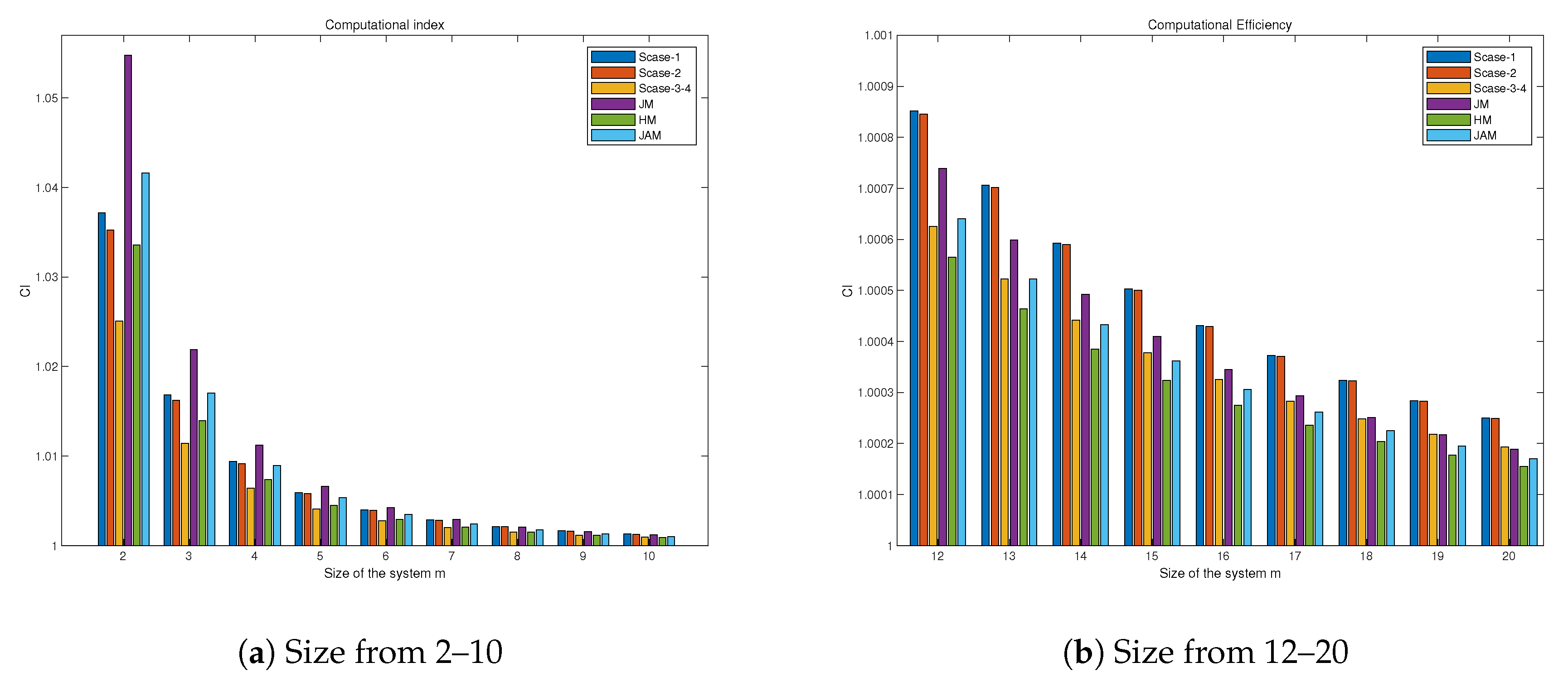
We observe that, although index I is the same in all these cases, this is not the case of index $CI$, since the number of inverse linear operators is different for each scheme. In Figure 1, index $CI$ for those methods and systems of size from 2–20 is shown. We can observe that, for a size of the system greater than eight, the best index corresponds to the proposed methods Scase-1 and Scase-2, due to the number of linear systems to be solved and the factor of the dominating term, that is $\frac{1}{3}{m}^3$, in comparison to $\frac{2}{3}{m}^3$ in other schemes.

4. Numerical Examples

In this section, we show the effectiveness and efficiency of some of our proposed methods, and we compare them with other existing optimal (scalar case) iterative schemes of the same order. In the one-dimensional case, for comparison purposes, we consider some cases from Table 1, Case-1, Case-3 $\left(\mathrm{for}a=\frac{1}{10},b=3\right)$, Case-4 (for $a=10$ and $b=2$), and Case-5 (for $a=1$ and $b=1$), called $OM1$, $OM2$, $OM3$, and $OM4$, respectively. In addition, we consider three real-life problems, e.g., a chemical engineering problem, the movement of an electron in the air space between two parallel plates, and the fractional conversion in a chemical reactor problem, which are displayed in Examples 1–3. In addition, the solution to the corresponding problem is also listed in the corresponding example, which is correct up to 30 significant digits. However, the desired roots are available up to several significant digits (a minimum of one thousand), but due the page limit restriction, only 30 significant digits are displayed.

Now, we compare them with the optimal fourth-order multi-point iteration function proposed by Khattri and Abbasbandy [32] and Soleymani et al. [33]; from them, we considered methods (6) and (19) denoted as $(KA)$ and $(SKV)$, respectively. In addition, we also compare them with the optimal schemes of order four, which were presented by Chun [34] and King [35]; we have picked expressions (10) and (2) (for $\beta =1$) from them, called $(CM)$ and $(KM)$, respectively. Finally, we also compare them with another optimal family of fourth-order methods derived by Cordero et al. [36], from which we have chosen expression (9), called $(CHMT)$.

We compare our proposed methods with the existing ones in terms of the absolute residual error of the corresponding function $|f(x_n)|$, errors between the two consecutive iterations $|x_{n+1}-x_n|$, ${\displaystyle \left|\frac{x_{n+1}-x_n}{{(x_n-x_{n-1})}^4}\right|}$, and the asymptotic error constant ${\displaystyle \eta =\underset{n\to \infty }{lim}\left|\frac{x_{n+1}-x_n}{{(x_n-x_{n-1})}^4}\right|}$ in

Table 4. Convergence behavior of the different fourth-order optimal methods for $f_2(x)$.

Cases	n	${\mathit{x}}_{\mathit{n}}$	$|\mathit{f}({\mathit{x}}_{\mathit{n}})|$	$|{\mathit{x}}_{\mathit{n}+1}-{\mathit{x}}_{\mathit{n}}|$	$\left|\frac{{\mathit{x}}_{\mathit{n}+1}-{\mathit{x}}_{\mathit{n}}}{{({\mathit{x}}_{\mathit{n}}-{\mathit{x}}_{\mathit{n}-1})}^4}\right|$	$\mathit{\eta }$
$KA$	1	$4.06831779454242+0.32664091245691i$	$1.3(-)$	$1.2(-1)$
	2	$3.94566403244595+0.31195820042558i$	$5.1(-2)$	$5.1(-3)$	$2.8685$	$3.7507$
	3	$3.94854247724924+0.31612357071166i$	$3.2(-7)$	$3.7(-8)$	$3.7507$
$SKV$	1	$3.99435611429986+0.36507812608361i$	$7.5(-1)$	$6.7(-2)$
	2	$3.94874528304345+0.31606965860747i$	$2.1(-3)$	$2.1(-4)$	$3.7147$	$3.9136$
	3	$3.94854244556205+0.31612357089705i$	$3.4(-13)$	$3.3(-14)$	$3.9136$
$CM$	1	$3.98466616205972+0.38743296774392i$	$9.2(-1)$	$8.0(-2)$
	2	$3.94878185252247+0.31634115609934i$	$3.3(-3)$	$3.2(-4)$	$3.9938$	$3.9005$
	3	$3.94854244556214+0.31612357089689i$	$1.5(-12)$	$1.5(-13)$	$3.9005$
$KM$	1	$3.97985638724627+0.36440676727915i$	$6.4(-1)$	$5.7(-2)$
	2	$3.94863621913203+0.31615261583746i$	$9.9(-4)$	$9.8(-5)$	$3.8383$	$3.9314$
	3	$3.94854244556204+0.31612357089702i$	$1.3(-14)$	$1.3(-15)$	$3.9314$
$CHMT$	1	$4.00173953283203+0.36617288922003i$	$8.2(-1)$	$7.3(-2)$
	2	$3.94882489377247+0.31598753843337i$	$3.2(-3)$	$3.1(-4)$	$3.6593$	$3.9027$
	3	$3.94854244556219+0.31612357089712i$	$1.8(-12)$	$1.8(-13)$	$3.9027$
$OM1$	1	$4.01399307003023+0.35890761473628i$	$8.8(-1)$	$7.8(-2)$
	2	$3.94881862583921+0.31570149393965i$	$5.1(-3)$	$5.0(-4)$	$3.4856$	$3.8875$
	3	$3.94854244556209+0.31612357089548i$	$1.6(-11)$	$1.5(-12)$	$3.8875$
$OM2$	1	$4.12288139593880+0.38749751766959i$	$2.4(-)$	$2.2(-1)$
	2	$3.90767119668767+0.32432746535133i$	$4.2(-1)$	$4.2(-2)$	$2.4576$	$3.8283$
	3	$3.94858535174257+0.31617458259283i$	$6.7(-4)$	$6.7(-5)$	$3.8283$
$OM3$	1	$3.96901080029588+0.32053604782876i$	$2.2(-1)$	$2.1(-2)$
	2	$3.94854330300287+0.31612265035071i$	$1.3(-5)$	$1.3(-6)$	$3.7580$	$4.0300$
	3	$3.94854244556205+0.31612357089702i$	$1.2(-22)$	$1.2(-23)$	$4.0300$
$OM4$	1	$4.01399307003023+0.35890761473628i$	$8.8(-1)$	$7.8(-2)$
	2	$3.94881862583921+0.31570149393965i$	$5.1(-3)$	$5.0(-4)$	$3.4856$	$3.8875$
	3	$3.94854244556209+0.31612357089548i$	$1.6(-11)$	$1.5(-12)$	$3.8875$

,

Table 5. Convergence behavior of different fourth-order optimal methods for $f_3(x)$.

Cases	n	${\mathit{x}}_{\mathit{n}}$	$|\mathit{f}({\mathit{x}}_{\mathit{n}})|$	$|{\mathit{x}}_{\mathit{n}+1}-{\mathit{x}}_{\mathit{n}}|$	$\left|\frac{{\mathit{x}}_{\mathit{n}+1}-{\mathit{x}}_{\mathit{n}}}{{({\mathit{x}}_{\mathit{n}}-{\mathit{x}}_{\mathit{n}-1})}^4}\right|$	$\mathit{\eta }$
$KA$	1	$-0.25417804552034148536$	$4.7(-2)$	$5.5(-2)$
	2	$-0.30909163590606450952$	$1.4(-6)$	$1.6(-6)$	$3.3312$	$3.9907$
	3	$-0.30909327154179495274$	$1.2(-24)$	$1.4(-24)$	$3.9907$
$SKV$	1	$-1.9228013411768680913$	$9.7(-1)$	$1.9(+1)$
	2	$16.956846304184010120$	$1.8(+1)$	$5.7(+7)$	$7.9958$	$4.7137$
	3	$-5.6776688150342258615(+7)$	$5.7(+7)$	$2.0(+38)$	$4.7137$
$CM$	1	$-0.27247767593361877437$	$3.1(-2)$	$3.1(-2)$
	2	$-0.30909316991236159145$	$8.6(-8)$	$1.0(-7)$	$3.6059$	$3.9979$
	3	$-0.30909327154179495274$	$5.3(-30)$	$6.2(-30)$	$3.9979$
$KM$	1	$-0.27395213337785257000$	$3.0(-2)$	$3.5(-2)$
	2	$-0.30909318584556631521$	$7.3(-8)$	$8.6(-8)$	$3.5995$	$3.9975$
	3	$-0.30909327154179495274$	$2.7(-30)$	$3.1(-30)$	$3.9975$
$CHMT$	1	$-0.26958019693473408634$	$3.4(-2)$	$4.0(-2)$
	2	$-0.30909308449385539179$	$1.6(-7)$	$1.9(-7)$	$3.5336$	$3.9964$
	3	$-0.30909327154179495274$	$8.3(-29)$	$9.8(-29)$	$3.9964$
$OM1$	1	$-0.26631675279431609571$	$3.7(-1)$	$4.3(-2)$
	2	$-0.30909294799418381577$	$2.7(-7)$	$3.2(-7)$	$3.4807$	$3.9951$
	3	$-0.30909327154179495274$	$9.5(-28)$	$1.1(-27)$	$3.9951$
$OM2$	1	$-0.28888414806339401078$	$1.7(-2)$	$2.0(-2)$
	2	$-0.30909325486518945619$	$1.4(-8)$	$1.7(-8)$	$3.3709$	$3.9983$
	3	$-0.30909327154179495274$	$6.7(-33)$	$7.9(-33)$	$3.9983$
$OM3$	1	$-0.15994222854937208373$	$1.3(-1)$	$1.5(-1)$
	2	$-0.30899020010081667265$	$8.7(-5)$	$1.0(-4)$	$3.5463$	$3.9729$
	3	$-0.30909327154179492402$	$2.4(-17)$	$2.9(-17)$	$3.9729$
$OM4$	1	$-0.26631675279431609571$	$3.7(-2)$	$4.3(-2)$
	2	$-0.30909294799418381577$	$2.7(-7)$	$3.2(-7)$	$3.4807$	$3.9951$
	3	$-0.30909327154179495274$	$9.5(-28)$	$1.1(-27)$	$3.9951$

and

Table 6. Convergence behavior of different fourth-order optimal methods for $f_4(x)$.

Cases	n	${\mathit{x}}_{\mathit{n}}$	$|\mathit{f}({\mathit{x}}_{\mathit{n}})|$	$|{\mathit{x}}_{\mathit{n}+1}-{\mathit{x}}_{\mathit{n}}|$	$\left|\frac{{\mathit{x}}_{\mathit{n}+1}-{\mathit{x}}_{\mathit{n}}}{{({\mathit{x}}_{\mathit{n}}-{\mathit{x}}_{\mathit{n}-1})}^4}\right|$	$\mathit{\eta }$
$KA$	1	$0.75739764681484808246$	$1.1(-4)$	$1.4(-6)$
	2	$0.75739624625375387959$	$1.0(-17)$	$1.3(-19)$	$3.9858$	$4.0000$
	3	$0.75739624625375387946$	$7.9(-70)$	$9.9(-72)$	$4.0000$
$SKV$	1	$0.75739672982865568692$	$3.9(-5)$	$4.8(-7)$
	2	$0.75739624625375387946$	$4.8(-20)$	$6.0(-22)$	$3.9955$	$4.0000$
	3	$0.75739624625375387946$	$1.4(-79)$	$1.4(-81)$	$4.0000$
$CM$	1	$0.75739660630557206625$	$2.9(-5)$	$3.6(-7)$
	2	$0.75739624625375387946$	$1.0(-20)$	$1.3(-22)$	$4.0011$	$4.0000$
	3	$0.75739624625375387946$	$1.8(-82)$	$2.2(-84)$	$4.0000$
$KM$	1	$0.75739659212374876149$	$2.8(-5)$	$3.5(-7)$
	2	$0.75739624625375387946$	$8.9(-21)$	$1.1(-22)$	$3.9966$	$4.0000$
	3	$0.75739624625375387946$	$9.4(-83)$	$1.2(-84)$	$4.0000$
$CHMT$	1	$0.75739676303951339051$	$4.1(-5)$	$5.2(-7)$
	2	$0.75739624625375387946$	$6.7(-20)$	$8.4(-22)$	$3.9950$	$4.0000$
	3	$0.75739624625375387946$	$4.6(-79)$	$5.8(-81)$	$4.0000$
$OM1$	1	$0.75739692085844618425$	$5.4(-5)$	$6.7(-7)$
	2	$0.75739624625375387946$	$2.6(-19)$	$3.3(-21)$	$3.9917$	$4.0000$
	3	$0.75739624625375387946$	$1.4(-76)$	$1.8(-78)$	$4.0000$
$OM2$	1	$0.75739683227987612611$	$4.7(-5)$	$5.9(-7)$
	2	$0.75739624625375387946$	$1.5(-19)$	$1.9(-21)$	$3.9751$	$4.0000$
	3	$0.75739624625375387946$	$1.5(-77)$	$1.9(-79)$	$4.0000$
$OM3$	1	$0.75739622120709837787$	$2.0(-6)$	$2.5(-8)$
	2	$0.75739624625375387946$	$2.2(-27)$	$2.7(-29)$	$4.1779$	$4.0000$
	3	$0.75739624625375387946$	$3.2(-111)$	$4.0(-113)$	$4.0000$
$OM4$	1	$0.75739692085844618425$	$5.4(-5)$	$6.7(-7)$
	2	$0.75739624625375387946$	$2.6(-19)$	$3.3(-21)$	$3.9917$	$4.0000$
	3	$0.75739624625375387946$	$1.4(-76)$	$1.8(-78)$	$4.0000$

.

We calculate the asymptotic error constant and other constants up to several significant digits (a minimum of 1000 significant digits) to minimize the round-off error. We show the values of $x_n$, the absolute residual error in the function $|f(x_n)|$, the difference between the two consecutive iterations $|x_{n+1}-x_n|$, and the values of $\left|\frac{x_{n+1}-x_n}{{(x_n-x_{n-1})}^4}\right|$ and $\eta$.

In the context of nonlinear systems, we also consider two applied science problems to check further the validity of the theoretical results for the nonlinear system. We shall compare them with the methods, namely (14)–(16), called JM, HM, and JAM, respectively. We have included the number of iteration indexes $(n)$, the residual error of the corresponding function $(\parallel F(x^{(n+1)})\parallel )$, the error in the iterations $\parallel x^{(n+1)}-x^{(n)}\parallel$, and the approximated computational order of convergence $\rho =\frac{log\left[\parallel x^{(n+1)}-x^{(n)}\parallel /\parallel x^{(n)}-x^{(n-1)}\parallel \right]}{log\left[\parallel x^{(n)}-x^{(n-1)}\parallel /\parallel x^{(n-1)}-x^{(n-2)}\parallel \right]}$ (for details, see Cordero and Torregrosa [37]) in

Table 7. Convergence behavior of different fourth-order methods for Example 4.

Cases	n	$\parallel \mathit{F}({\mathit{x}}^{(\mathit{n}+1)})\parallel$	$\parallel {\mathit{x}}^{(\mathit{n}+1)}-{\mathit{x}}^{(\mathit{n})}\parallel$	$\mathit{\rho }$
Scase-1 $(a=1/200,b=3)$	1	$7.1(-9)$	$1.5(-9)$
	2	$5.5(-39)$	$1.2(-39)$
	3	$2.5(-159)$	$5.3(-160)$	$3.996$
Scase-2 $(a=1/200,b=3)$	1	$9.1(-9)$	$2.0(-9)$
	2	$1.9(-38)$	$4.0(-39)$
	3	$3.6(-157)$	$7.7(-158)$	$3.999$
Scase-3 $(a=1/200,b=3)$	1	$4.5(-7)$	$9.6(-8)$
	2	$1.6(-3)$	$3.4(-32)$
	3	$1.9(-129)$	$4.1(-130)$	$4.005$
Scase-4 $(a=1/200,b=3)$	1	$9.7(-9)$	$2.1(-9)$
	2	$2.4(-38)$	$5.2(-39)$
	3	$1.0(-156)$	$2.2(-157)$	$3.999$
JM	1	$5.9(-9)$	$1.3(-9)$
	2	$2.0(-39)$	$4.3(-40)$
	3	$2.9(-161)$	$6.2(-162)$	$3.999$
HM	1	$7.1(-9)$	$1.5(-9)$
	2	$5.4(-39)$	$1.2(-39)$
	3	$1.8(-159)$	$3.8(-160)$	$3.999$
JAM	1	$7.1(-9)$	$1.5(-9)$
	2	$5.4(-39)$	$1.2(-39)$
	3	$1.8(-159)$	$3.8(-160)$	$3.999$

and

Table 8. Convergence behavior of different fourth-order methods for Example 5.

Cases	n	$\parallel \mathit{F}({\mathit{x}}^{(\mathit{n}+1)})\parallel$	$\parallel {\mathit{x}}^{(\mathit{n}+1)}-{\mathit{x}}^{(\mathit{n})}\parallel$	$\mathit{\rho }$
Scase-1 $(a=1/200,b=3)$	1	$1.8(-5)$	$3.3(-5)$
	2	$1.2(-22)$	$2.4(-22)$
	3	$2.9(-91)$	$6.2(-91)$	$4.000$
Scase-2 $(a=1/200,b=3)$	1	$3.4(-5)$	$4.0(-5)$
	2	$2.5(-22)$	$3.9(-22)$
	3	$2.0(-90)$	$3.8(-90)$	$3.998$
Scase-3 $(a=1/200,b=3)$	1	$1.2(-5)$	$2.1(-5)$
	2	$1.5(-23)$	$3.0(-23)$
	3	$7.0(-95)$	$1.5(-94)$	$3.998$
Scase-4 $(a=1/200,b=3)$	1	$3.2(-5)$	$4.0(-5)$
	2	$2.5(-22)$	$4.0(-22)$
	3	$2.2(-90)$	$4.3(-90)$	$3.998$
JM	1	$2.8(-5)$	$4.0(-5)$
	2	$3.5(-22)$	$6.2(-22)$
	3	$1.8(-89)$	$3.7(-89)$	$3.998$
HM	1	$2.7(-5)$	$3.9(-5)$
	2	$2.8(-22)$	$5.1(-22)$
	3	$7.3(-90)$	$1.5(-89)$	$3.998$
JAM	1	$2.7(-5)$	$3.9(-5)$
	2	$2.8(-22)$	$5.1(-22)$
	3	$7.3(-90)$	$1.5(-89)$	$3.998$

.

All computations have been performed using the software Mathematica 9 (Wolfram Research, Champaign, IL, USA) with multiple precision arithmetic, and in Table 4, Table 5, Table 6, Table 7 and Table 8, $A(\pm B)$ denotes the number $A\times {10}^{(\pm B)}$.

Example 1.

We consider a quartic equation from Shacham, Balaji, and Seader [1,2], which describes the fractional conversion, that is the fraction of the nitrogen-hydrogen feed getting converted to ammonia. If we consider 250 atm and 500 ${}^{\circ }$C, then the equation has the form:

$$f_2(z)=z^4-7.79075z^3+14.7445z^2+2.511z-1.674.$$

(17)

Function (17) has four zeros, two real zeros, and two conjugated complexes. We want to obtain the zero $x^{*}\approx 3.9485424455620457727+0.3161235708970163733i$ with initial approximation $x_0=3.7+0.25i$. Other initial approaches further away from the solution give similar numerical results, with a slower approach to the solution.

Example 2.

In the analysis of the movement of an electron in the air gap between two parallel plates, the multi-factor effect is given by:

$$\begin{array}{cc}\hfill p(t)=& p_0+\left(v_0+e\frac{E_0}{m\omega }sin(\omega t_0+\alpha )\right)(t-t_0)+e\frac{E_0}{m{\omega }^2}\left(cos(\omega t+\alpha )+sin(\omega +\alpha )\right),\hfill \end{array}$$

(18)

e and m, respectively, being the charge and the mass of the electron, $p_0$ and $v_0$ being, respectively, the position and velocity of the electron at instant $t_0$, and also $E_{0}sin(\omega t+\alpha )$ being the RF electric field between the plates. By selecting some values of the parameters in Equation (17), to simplify the expression, we obtain:

$$f_3(x)=x-\frac{1}{2}cos(x)+\frac{\pi }{4}.$$

(19)

This function has a simple zero at $x^{*}\approx -0.309093271541794952741986808924$, and we use the initial estimation of one.

Example 3.

In expression (see [3]),

$$f_4(x)=\frac{x}{1-x}-5log\left[\frac{0.4(1-x)}{0.4-0.5x}\right]+4.45977,$$

(20)

where x denotes the fractional conversion of Species A in a chemical reactor. We must take into account that there is no physical meaning to this expression if $x<0$ or $x>1$. Then, x is considered in the interval $0\le x\le 1$. The searched zero is $x^{*}\approx 0.757396246253753879459641297929$. Indeed, let us remark that expression (20) is undefined in $0.8\le x\le 1$, very near to the zero. The derivative of expression (20) is close to zero in $0\le x\le 0.5$. Therefore, we consider the initial approximation to be $x_0=0.76$ for this problem.

Example 4.

Considering the mixed Hammerstein integral equation, from Ortega and Rheinbolt [10], given by:

$$x(s)=1+\frac{1}{5}{\int }_0^{1}G(s,t)x{(t)}^{3}dt$$

(21)

where $x\in C[0,1]$, s, and t belong to $[0,1]$, and kernel G is defined as $(1-s)t$ if $t\le s$ and as $s(1-t)$ when $s\le t$.

We use the Gauss-Legendre quadrature formula with ten nodes $t_j$ and weights $w_j$ (see

Table 9. Values of abscissas $t_j$ and weights $w_j$.

j	${\mathit{t}}_{\mathit{j}}$	${\mathit{w}}_{\mathit{j}}$
1	$0.01304673574141413996101799$	$0.03333567215434406879678440$
2	$0.06746831665550774463395165$	$0.07472567457529029657288816$
3	$0.16029521585048779688283632$	$0.10954318125799102199776746$
4	$0.28330230293537640460036703$	$0.13463335965499817754561346$
5	$0.42556283050918439455758700$	$0.14776211235737643508694649$
6	$0.57443716949081560544241300$	$0.14776211235737643508694649$
7	$0.71669769706462359539963297$	$0.13463335965499817754561346$
8	$0.83970478414951220311716368$	$0.10954318125799102199776746$
9	$0.93253168334449225536604834$	$0.07472567457529029657288816$
10	$0.98695326425858586003898201$	$0.03333567215434406879678440$

), $j=1,2,\dots ,10$, to transform the integral equation into a nonlinear system. By denoting the approximations of $x(t_i)$ by $x_i$, $i=1,2,\dots ,10$, one gets the nonlinear system:

$${\displaystyle 5x_i-5-\sum _{j=1}^{10}{a}_{ij}{x}_j^3=0,}$$

where $i=1,2,\dots ,10$, and:

$$a_{ij}=\left\{\begin{array}{c}\hfill w_j{t}_j(1-t_i),j\le i,\\ \hfill w_j{t}_i(1-t_j),i<j,\end{array}\right.$$

In Table 7, we show the numerical results obtained by using $x_0={(1,1,\cdots ,1)}^T$ to search the root:

$$\overline{x}\approx {(1.0013\dots ,1.0067\dots ,1.0145\dots ,1.0219\dots ,1.0265\dots ,1.0265\dots ,1.0219\dots ,1.0145\dots ,1.0067\dots ,1.0013\dots )}^T.$$

Example 5.

Let us consider the following boundary value problem described in [10]:

$$y^{″}=\frac{1}{2}{y}^3+3y^{\prime }-\frac{3}{2-x}+\frac{1}{2},y(0)=0,y(1)=1.$$

(22)

We partition the interval $[0,1]$ as follows:

$$x_0=0<x_1<x_2<x_3<\cdots <x_n,\mathrm{where}{x}_{i+1}=x_i+h,h=\frac{1}{n},$$

and we also consider $y_0=y(x_0)=0,y_1=y(x_1),\cdots ,y_{n-1}=y(x_{n-1}),y_n=y(x_n)=1$. Now, we discretize problem (22) by using the following approximations of the derivatives:

$$y_j^{\prime }\approx \frac{y_{j+1}-y_{j-1}}{2h},y_j^{″}\approx \frac{y_{j-1}-2y_j+y_{j+1}}{h^2},j=1,2,\cdots ,n-1.$$

Therefore, a nonlinear system of size $(n-1)\times (n-1)$ is obtained:

$$y_{j+1}-2y_j+y_{j-1}-\frac{h^2}{2}{y}_j^3-\frac{3}{2-x_j}{h}^2-3\frac{y_{j+1}-y_{j-1}}{2}h-\frac{1}{h^2}=0,k=1,2,\dots ,n-1.$$

If we use the initial guess $y^{(0)}={\left(\frac{1}{10},\frac{1}{10},\frac{1}{10},\frac{1}{10},\frac{1}{10},\frac{1}{10}\right)}^T$, to solve the nonlinear system obtained for $n=7$, we obtain the solution:

$$\overline{x}\approx {\left(0.07654393\dots ,0.1658739\dots ,0.2715210\dots ,0.3984540\dots ,0.5538864\dots ,0.7486878\dots \right)}^T,$$

and the numerical results are shown in Table 8.

Results and Discussion

We can say from Table 4, Table 5 and Table 6 that our methods had smaller residual error, in each test function, than the known methods used for comparison, namely $KA$, $SKV$, $CM$, $KM$, and $CHMT$. In addition, our methods also had a smaller distance between two consecutive iterations. Therefore, our method converged faster towards the exact root as compared to the existing ones. On the other hand, the proposed methods also had a simple asymptotic error constant corresponding to each test function, which can be seen in Table 4, Table 5 and Table 6. A similar type of behavior of our methods was found in the case of the multidimensional extension, which is mentioned in Table 7 and Table 8. However, our methods could have different behaviors depending on the nonlinear equation. Actually, the behavior of the iterative methods mainly depended on the complexity of the iterative expression, the test function used, the initial guess, the programming of the scheme, etc.

5. Conclusions

In the past, several researchers proposed optimal multi-point fourth-order iterative methods for simple roots of nonlinear equations, by using weight functions or free parameters only in the second scheme. In this paper, we design a family of two-step optimal iterative methods with fourth-order convergence, including weight functions and parameters in the two steps of the methods. The main strength of our proposed schemes is that they not only give flexibility to researchers at both steps for constructing new optimal fourth-order methods, but also give a faster convergence, a small residual error corresponding to the involved function, and asymptotic error constants in relation to other known schemes. In addition of this, the local convergence analysis of the suggested schemes was proven through Lipschitz constants and the Banach lemma in order to calculate the local convergence radius. Moreover, we extended the proposed scheme to systems of nonlinear equations, preserving the same order of convergence and the same beauty that the scalar one has. Numerical results were performed and compared with earlier existing methods. The results were very consistent with the existing methods.

References

- Shacham, M. An improved memory method for the solution of a nonlinear equation. Chem. Eng. Sci. 1989, 44, 1495–1501. [Google Scholar] [CrossRef]
- Balaji, G.V.; Seader, J.D. Application of interval Newton’s method to chemical engineering problems. Reliab. Comput. 1995, 1, 215–223. [Google Scholar] [CrossRef]
- Shacham, M. Numerical solution of constrained nonlinear algebraic equations. Int. J. Numer. Method Eng. 1986, 23, 1455–1481. [Google Scholar] [CrossRef]
- Shacham, M.; Kehat, E. Converging interval methods for the iterative solution of nonlinear equations. Chem. Eng. Sci. 1973, 28, 2187–2193. [Google Scholar] [CrossRef]
- Moré, J.J. A Collection of Nonlinear Model Problems; Lectures in Applied Mathematics; American Mathematical Society: Providence, RI, USA, 1990; Volume 26, pp. 723–762. [Google Scholar]
- Grosan, C.; Abraham, A. A new approach for solving nonlinear equations systems. IEEE Trans. Syst. Man Cyber. Part A Syst. Hum. 2008, 38, 698–714. [Google Scholar] [CrossRef]
- Awawdeh, F. On new iterative method for solving systems of nonlinear equations. Numer. Algorithms 2010, 54, 395–409. [Google Scholar] [CrossRef]
- Tsoulos, I.G.; Stavrakoudis, A. On locating all roots of systems of nonlinear equations inside bounded domain using global optimization methods. Nonlinear Anal. Real World Appl. 2010, 11, 2465–2471. [Google Scholar] [CrossRef]
- Lin, Y.; Bao, L.; Jia, X. Convergence analysis of a variant of the Newton method for solving nonlinear equations. Comput. Math. Appl. 2010, 59, 2121–2127. [Google Scholar] [CrossRef]
- Ortega, J.M.; Rheinbolt, W.C. Iterative Solutions of Nonlinears Equations in Several Variables; Academic Press: Cambridge, MA, USA, 1970. [Google Scholar]
- Petković, M.S.; Neta, B.; Petković, L.D.; Dz̆unić, J. Multipoint Methods for Solving Nonlinear Equations; Academic Press: Cambridge, MA, USA, 2013. [Google Scholar]
- Traub, J.F. Iterative Methods for the Solution of Equations; Prentice-Hall: Englewood Cliffs, NJ, USA, 1964. [Google Scholar]
- Amat, S.; Busquier, S. Advances in Iterative Methods for Nonlinear Equations; SEMA SIMAI Springer Series; Springer: Berlin, Germany, 2016; Volume 10. [Google Scholar]
- Nedzhibov, G.H. A family of multi-point iterative methods for solving systems of nonlinear equations. J. Comput. Appl. Math. 2008, 222, 244–250. [Google Scholar] [CrossRef]
- Jarratt, P. Some fourth-order multipoint iterative methods for solving equations. Math. Comput. 1966, 20, 434–437. [Google Scholar] [CrossRef]
- Khan, W.A.; Noor, K.I.; Bhattia, K.; Ansari, F.A. A new fourth order Newton-type method for solution of system of nonlinear equations. Appl. Math. Comput. 2015, 270, 724–730. [Google Scholar] [CrossRef]
- Hueso, J.L.; Martínez, E.; Teruel, C. Convergence, Efficiency and Dynamics of new fourth and sixth order families of iterative methods for nonlinear systems. J. Comput. Appl. Math. 2015, 275, 412–420. [Google Scholar] [CrossRef]
- Junjua, M.; Akram, S.; Yasmin, N.; Zafar, F. A New Jarratt-Type Fourth-Order Method for Solving System of Nonlinear Equations and Applications. Appl. Math. 2015, 2015, 805278. [Google Scholar] [CrossRef]
- Gutiérrez, J.M.; Hernández, M.A. An acceleration of Newton’s method: Super-Halley method in a Banach space. Appl. Math. Comput. 2001, 117, 223–239. [Google Scholar]
- Chun, C. Some second-derivative-free variants of Chebyshev’s Halley methods. Appl. Math. Comput. 2007, 191, 410–414. [Google Scholar]
- Kou, J.; Li, Y.; Wang, X. Fourth-order iterative methods free from second derivative. Appl. Math. Comput. 2007, 184, 880–885. [Google Scholar] [CrossRef]
- Noor, M.A.; Ahmad, F. Fourth-order convergent iterative method for nonlinear equation. Appl. Math. Comput. 2006, 182, 1149–1153. [Google Scholar] [CrossRef]
- Sharma, J.R.; Guha, R.K.; Sharma, R. Some variants of Hansen-Patrick method with third and fourth order convergence. Appl. Math. Comput. 2009, 214, 171–177. [Google Scholar] [CrossRef]
- Chun, C.; Neta, B. Certain improvement of Newton’s method with fourth-order convergence. Appl. Math. Comput. 2009, 215, 821–828. [Google Scholar] [CrossRef]
- Kung, H.T.; Traub, J.F. Optimal order of one-point and multi-point iteration. J. ACM 1974, 21, 643–651. [Google Scholar] [CrossRef]
- Abad, M.F.; Cordero, A.; Torregrosa, J.R. A family of seventh-order schemes for solving nonlinear systems. Bull. Math. Soc. Sci. Math. Roum. 2014, 57, 133–145. [Google Scholar]
- Cordero, A.; Maimó, J.G.; Torregrosa, J.R.; Vassileva, M.P. Solving nonlinear problems by Ostrowski-Chun type parametric families. Math. Chem. 2014, 52, 430–449. [Google Scholar]
- Hermite, C. Sur la formule d’interpolation de Lagrange. Reine Angew. Math. 1878, 84, 70–79. [Google Scholar] [CrossRef]
- Cordero, A.; Hueso, J.L.; Martínez, E.; Torregrosa, J.R. A modified Newton-Jarratt’s composition. Numer. Algorithms 2010, 55, 87–99. [Google Scholar] [CrossRef]
- Sharma, J.R.; Arora, H. On efficient weighted-Newton methods for solving systems of nonlinear equations. Appl. Math. Comput. 2013, 222, 497–506. [Google Scholar] [CrossRef]
- Ostrowski, A.M. Solution of Equations and Systems of Equations; Prentice-Hall: Englewood Cliffs, NJ, USA; New York, NY, USA, 1964. [Google Scholar]
- Khattri, S.K.; Abbasbandy, S. Optimal fourth order family of iterative methods. Mat. Vesnik 2011, 63, 67–72. [Google Scholar]
- Soleymani, F.; Khattri, S.K.; Vanani, S.K. Two new classes of optimal Jarratt-type fourth-order methods. Appl. Math. Lett. 2012, 25, 847–853. [Google Scholar] [CrossRef]
- Chun, C. Some variants of King’s fourth-order family of methods for nonlinear equations. Appl. Math. Comput. 2007, 190, 57–62. [Google Scholar] [CrossRef]
- King, R.F. A family of fourth order methods for nonlinear equations. SIAM Numer. Anal. 1973, 10, 876–879. [Google Scholar] [CrossRef]
- Cordero, A.; Hueso, J.L.; Martínez, E.; Torregrosa, J.R. New modifications of Potra-Pták’s method with optimal fourth and eighth orders of convergence. Comput. Appl. Math. 2010, 234, 2969–2976. [Google Scholar] [CrossRef]
- Cordero, A.; Torregrosa, J.R. Variants of Newton’s method using fifth-order quadrature formulas. Appl. Math. Comput. 2007, 190, 686–698. [Google Scholar] [CrossRef]
Figure 1.
Index for different sizes of the system.