Forecast-Triggered Model Predictive Control of Constrained Nonlinear Processes with Control Actuator Faults

Abstract

This paper addresses the problem of fault-tolerant stabilization of nonlinear processes subject to input constraints, control actuator faults and limited sensor–controller communication. A fault-tolerant Lyapunov-based model predictive control (MPC) formulation that enforces the fault-tolerant stabilization objective with reduced sensor–controller communication needs is developed. In the proposed formulation, the control action is obtained through the online solution of a finite-horizon optimal control problem based on an uncertain model of the plant. The optimization problem is solved in a receding horizon fashion subject to appropriate Lyapunov-based stability constraints which are designed to ensure that the desired stability and performance properties of the closed-loop system are met in the presence of faults. The state-space region where fault-tolerant stabilization is guaranteed is explicitly characterized in terms of the fault magnitude, the size of the plant-model mismatch and the choice of controller design parameters. To achieve the control objective with minimal sensor–controller communication, a forecast-triggered communication strategy is developed to determine when sensor–controller communication can be suspended and when it should be restored. In this strategy, transmission of the sensor measurement at a given sampling time over the sensor–controller communication channel to update the model state in the predictive controller is triggered only when the Lyapunov function or its time-derivative are forecasted to breach certain thresholds over the next sampling interval. The communication-triggering thresholds are derived from a Lyapunov stability analysis and are explicitly parameterized in terms of the fault size and a suitable fault accommodation parameter. Based on this characterization, fault accommodation strategies that guarantee closed-loop stability while simultaneously optimizing control and communication system resources are devised. Finally, a simulation case study involving a chemical process example is presented to illustrate the implementation and evaluate the efficacy of the developed fault-tolerant MPC formulation.

1. Introduction

Model predictive control (MPC), also known as receding horizon control, refers to a class of optimization-based control algorithms that utilize an explicit process model to predict the future response of the plant. At each sampling time, a finite-horizon optimal control problem with a cost functional that captures the desired performance requirements is solved subject to state and control constraints, and a sequence of control actions over the optimization horizon is generated. The first part of the control inputs in the sequence is implemented on the plant, and the optimization problem is solved repeatedly at every sampling time. While developed originally in response to the specialized control needs of large-scale industrial systems, such as petroleum refineries and power plants, MPC technology now spans a broad range of application areas including chemicals, food processing, automotive, and aerospace applications (see, for example, [1]). Motivated by the advantages of MPC, such as constraint handling capabilities, performance optimization, handling multi-variable interactions and ease of implementation, an extensive and growing body of research has been developed over the past few decades on the analysis, design and implementation of MPC, leading to a plethora of MPC formulations (see, for example, References [2,3,4] for some recent research directions and references in the field).

With the increasing demand over the past few decades for meeting stringent stability and performance specifications in industrial operations, fault-tolerance capabilities have become an increasingly important requirement in the design and implementation of modern day control systems. This is especially the case for safety-critical applications, such as chemical processes, where malfunctions in the control devices or process equipment can cause instabilities and lead to safety hazards if not appropriately mitigated through the use of fault-tolerant control approaches (see, for example, References [5,6,7] for some results and references on fault-tolerant control). The need for fault-tolerant control is further underscored by the increasing calls in recent times to achieve zero-incident plant operations as part of enabling the transition to smart plant operations ([8]).

As an advanced controller design methodology, MPC is also faced with the challenges of dealing with faults and handling the resulting degradation in the closed-loop stability and performance properties. Not surprisingly, this problem has been the subject of significant research work, and various methods have been investigated for the design and implementation of fault-tolerant MPC for both linear and nonlinear processes (see, for example, References [9,10,11,12,13] for some results and references in this area). An examination of the available literature on fault-tolerant MPC, however, reveals that the majority of existing methods have been developed within the traditional feedback control setting which assumes that the sensor–controller communication takes place over reliable dedicated links with flawless data transfer. This assumption needs to be re-examined in light of the widespread reliance on networked control systems which are characterized by increased levels of integration of resource-limited communication networks in the feedback loop.

The need to address the control-relevant challenges introduced by the intrinsic limitations on the processing and transmission capabilities of the sensor–controller communication medium has motivated a significant body of research work on networked control systems. Examples of efforts aimed at addressing some of these challenges in the context of MPC include the results in [14,15] where resource-aware MPC formulations that guarantee closed-loop stability with reduced sensor–controller communication requirements have been developed using event-based control techniques. In these studies, however, the problem of integrating fault-tolerance capabilities in the MPC design framework was not addressed.

Motivated by the above considerations, the aim of this work is to present a methodology for the design and implementation of fault-tolerant MPC for nonlinear process systems subject to model uncertainties, input constraints, control actuator faults and sensor–controller communication constraints. The co-presence of faults, control and communication resource constraints creates a conflict in the control design objectives where, on the one hand, increased levels of sensor–controller communication may be needed to mitigate the effects of the faults, and, on the other, such levels may be either unattainable or undesirable due to the sensor–controller communication constraints. To reconcile these conflicting objectives, a resource-aware Lyapunov-based MPC formulation that achieves the fault-tolerant stabilization objective with reduced sensor–controller communication is presented in this work.

The remainder of the paper is organized as follows. Section 2 begins by introducing some preliminaries that define the scope of the work and the class of systems considered. Section 3 then introduces an auxiliary Lyapunov-based fault-tolerant controller synthesized on the basis of an uncertain model of the plant and characterizes its closed-loop stability region. An analysis of the effects of discrete measurement sampling on the stability properties of the closed-loop model is conducted using Lyapuonv techniques and subsequently used in Section 4 to formulate a Lyapunov-based MPC that retains the same closed-loop stability and fault-tolerance properties enforced by the auxiliary model-based controller. The stability properties of the closed-loop system are analyzed and precise conditions that guarantee ultimate boundedness of the closed-loop trajectories in the presence of faults, discretely-sampled measurements and plant-model mismatch are provided. A forecasting scheme is then developed to predict the evolution of the Lyapunov function and its time-derivative over each sampling interval. The forecasts are used to trigger updates of the model states using the actual state measurements whenever certain stability-based thresholds are projected to be breached. Finally, Section 6 presents a simulation study that demonstrates the implementation and efficacy of the developed MPC formulation.

2. Preliminaries

We consider the class of finite-dimensional nonlinear process systems with the following state-space representation:

$$\dot{\mathbf{x}}=\mathbf{f}\left(\mathbf{x}\right)+\mathbf{G}\left(\mathbf{x}\right)\mathsf{\Theta }\mathbf{u}$$

(1)

where $\mathbf{x}\in {\mathbb{R}}^{n_{\mathbf{x}}}$ is the vector of process state variables, and $\mathbf{f}(·)$ and $\mathbf{G}(·)$ are sufficiently smooth nonlinear functions of their arguments on the domain of interest which contains the origin in its interior. Without loss of generality, the origin is assumed to be an equilibrium point of the uncontrolled plant (i.e., $\mathbf{f}\left(\mathbf{0}\right)=\mathbf{0}$). The matrix $\mathsf{\Theta }=\mathrm{diag}\{{\theta }_1{\theta }_2\cdots {\theta }_m\}$ is a diagonal deterministic (but unknown) fault coefficient matrix, where ${\theta }_i$ is a fault parameter whose value indicates the fault or health status of the i-th control actuator. A value of ${\theta }_i=1$ indicates that the i-th actuator is perfectly healthy, whereas a value of ${\theta }_i=0$ represents a completely failed (non-functioning) control actuator. Any other value, ${\theta }_i\in (0,1)$, represents a certain degree of fault. The parameter ${\theta }_i$ essentially measures the effectiveness (or control authority) of the i-th control actuator, with ${\theta }_i=0$ indicating an ineffective failed actuator, ${\theta }_i=1$ indicating a fully effective actuator, and any other value indicating a partially effective actuator that implements only a fraction of the required control action prescribed by the controller. The vector of manipulated input variables, $\mathbf{u}\in {\mathbb{R}}^{n_{\mathbf{u}}}$, takes values in a nonempty compact convex set $\mathcal{U}\triangleq \{\mathbf{u}\in {\mathbb{R}}^{n_{\mathbf{u}}}:\parallel \mathbf{u}\parallel \le u^{\max }\}$ where $u^{\max }>0$ represents the magnitude of input constraints and $\parallel ·\parallel$ denotes the Euclidean norm of a vector or matrix.

The control objective is to steer the process state from a given initial condition to the origin in the presence of input constraints, control actuator faults and limited sensor–controller communication. To facilitate controller synthesis, we assume that an uncertain dynamic model of the system of Equation (1) is available and has the following form:

$$\dot{\widehat{\mathbf{x}}}=\widehat{\mathbf{f}}\left(\widehat{\mathbf{x}}\right)+\widehat{\mathbf{G}}\left(\widehat{\mathbf{x}}\right)\widehat{\mathsf{\Theta }}\mathbf{u}$$

(2)

where $\widehat{\mathbf{x}}$ is the model state, $\widehat{\mathbf{f}}(·)$ and $\widehat{\mathbf{G}}(·)$ are sufficiently smooth nonlinear functions that approximate the functions $\mathbf{f}(·)$ and $\mathbf{G}(·)$, respectively, in Equation (1), and are given by:

$$\begin{array}{cc}\hfill \widehat{\mathbf{f}}\left(\mathbf{x}\right)& =\mathbf{f}\left(\mathbf{x}\right)+{\delta }_{\mathbf{f}}\left(\mathbf{x}\right)\hfill \end{array}$$

(3a)

$$\begin{array}{cc}\hfill \widehat{\mathbf{G}}\left(\mathbf{x}\right)& =\mathbf{G}\left(\mathbf{x}\right)-{\delta }_{\mathbf{G}}\left(\mathbf{x}\right)\hfill \end{array}$$

(3b)

where ${\delta }_{\mathbf{f}}(·)$ and ${\delta }_{\mathbf{G}}(·)$ are smooth nonlinear functions that capture the model uncertainties, and the following Lipschitz conditions hold on a certain region of interest:

$$\begin{array}{cc}\hfill \parallel \widehat{\mathbf{f}}\left({\mathbf{x}}_1\right)-\widehat{\mathbf{f}}\left({\mathbf{x}}_2\right)\parallel & \le {\widehat{L}}_1\parallel {\mathbf{x}}_1-{\mathbf{x}}_2\parallel \hfill \end{array}$$

(4a)

$$\begin{array}{cc}\hfill \parallel \widehat{\mathbf{G}}\left({\mathbf{x}}_1\right)-\widehat{\mathbf{G}}\left({\mathbf{x}}_2\right)\parallel & \le {\widehat{L}}_2\parallel {\mathbf{x}}_1-{\mathbf{x}}_2\parallel \hfill \end{array}$$

(4b)

where ${\widehat{L}}_1$ and ${\widehat{L}}_2$ are known positive constants. $\widehat{\mathsf{\Theta }}=\mathrm{diag}\{{\widehat{\theta }}_1{\widehat{\theta }}_2\cdots {\widehat{\theta }}_m\}$ is a diagonal matrix, where ${\widehat{\theta }}_i$ is an estimate of the actual fault coefficient, ${\theta }_i$. As discussed below, ${\widehat{\theta }}_i$ can also be viewed as a fault accommodation parameter that can be adjusted within the model to help achieve the fault-tolerant stabilization objective.

Towards our goal of designing a fault-tolerant MPC with well-characterized stability and performance properties, we begin in the next section by introducing an auxiliary bounded Lyapunov-based fault-tolerant controller that has an explicitly-characterized region of stability in the presence of faults. The stability properties of this controller are used as the basis for the development of a Lyapunov-based MPC formulation that retains the same closed-loop stability and fault-tolerance characteristics.

3. An Auxiliary Model-Based Fault-Tolerant Controller

3.1. Controller Synthesis and Analysis under Continuous State Measurements

Based on the dynamic model of Equation (2), we consider the following bounded Lyapunov-based state feedback controller:

$$\begin{array}{cc}\hfill \mathbf{u}\left(\widehat{\mathbf{x}}\right)& =-k(\widehat{\mathbf{x}},\widehat{\mathsf{\Theta }}){(L_{\widehat{\mathbf{G}}}V\left(\widehat{\mathbf{x}}\right)\widehat{\mathsf{\Theta }})}^T\doteq \mathbf{k}(\widehat{\mathbf{x}},\widehat{\mathsf{\Theta }})\hfill \end{array}$$

(5a)

$$\begin{array}{cc}\hfill k(\widehat{\mathbf{x}},\widehat{\mathsf{\Theta }})& =\frac{\alpha \left(\widehat{\mathbf{x}}\right)+\sqrt{{\left(\alpha \left(\widehat{\mathbf{x}}\right)\right)}^2+(u^{\max }\parallel {\beta }^T(\widehat{\mathsf{\Theta }},\widehat{\mathbf{x}}){\parallel )}^4}}{\parallel {\beta }^T(\widehat{\mathsf{\Theta }},\widehat{\mathbf{x}}){\parallel }^2[1+\sqrt{1+(u^{\max }\parallel {\beta }^T(\widehat{\mathsf{\Theta }},\widehat{\mathbf{x}}){\parallel )}^2} ]}\hfill \end{array}$$

(5b)

$$\begin{array}{cc}\hfill \alpha \left(\widehat{\mathbf{x}}\right)& \doteq L_{\widehat{\mathbf{f}}}V+\lambda V=\frac{\partial V}{\partial \widehat{\mathbf{x}}}\widehat{\mathbf{f}}+\lambda V\hfill \end{array}$$

(5c)

$$\begin{array}{cc}\hfill \beta (\widehat{\mathsf{\Theta }},\widehat{\mathbf{x}})& \doteq L_{\widehat{\mathbf{G}}}V\left(\widehat{\mathbf{x}}\right)\widehat{\mathsf{\Theta }},L_{\widehat{\mathbf{G}}}V=[\frac{\partial V}{\partial \widehat{\mathbf{x}}}{\widehat{\mathbf{g}}}^1\cdots \frac{\partial V}{\partial \widehat{\mathbf{x}}}{\widehat{\mathbf{g}}}^m]\hfill \end{array}$$

(5d)

where $L_{\widehat{\mathbf{f}}}V$ and $L_{\widehat{\mathbf{G}}}V$ are the Lie derivatives of V with respect to, $\widehat{\mathbf{f}}$ and $\widehat{\mathbf{G}}$, respectively; V is a control Lyapunov function that satisfies the following inequalities:

$$\begin{array}{cc}\hfill {\alpha }_1\left(\parallel \widehat{\mathbf{x}}\parallel \right)\le V\left(\widehat{\mathbf{x}}\right)& \le {\alpha }_2\left(\parallel \widehat{\mathbf{x}}\parallel \right)\hfill \end{array}$$

(6a)

$$\begin{array}{cc}\hfill ∥\frac{\partial V\left(\widehat{\mathbf{x}}\right)}{\partial \widehat{\mathbf{x}}}∥& \le {\alpha }_3\left(\parallel \widehat{\mathbf{x}}\parallel \right)\hfill \end{array}$$

(6b)

$$\begin{array}{cc}\hfill ∥\frac{\partial V\left(\widehat{\mathbf{x}}\right)}{\partial \widehat{\mathbf{x}}}\widehat{\mathbf{G}}\left(\widehat{\mathbf{x}}\right)∥& \le {\alpha }_4(\parallel \widehat{\mathbf{x}}\parallel )\hfill \end{array}$$

(6c)

for some class $\mathcal{K}$ functions (A function $\alpha (·)$ is said to be of class $\mathcal{K}$ if it is strictly increasing and $\alpha \left(0\right)=0$) ${\alpha }_i(·),i\in \{1,2,3,4\}$ and $\lambda$ is a controller design parameter. The controller of Equation (5) belongs to the general class of constructive nonlinear controllers referred to in the literature as Sontag-type controllers. Similar to earlier bounded controller designs (see, for example, [16]), it is obtained by scaling Sontag’s original universal formula to ensure that the control constraints are met within a certain well-defined region of the state space. The controller in Equation (5), however, differs from earlier designs in that it incorporates the fault explicitly into the controller synthesis formula.

It can be shown (see [16] for a similar proof) that the controller of Equation (5) satisfies the control constraints within a well-defined region in the state space, i.e.,:

$$\parallel \mathbf{k}(\widehat{\mathbf{x}},\widehat{\mathsf{\Theta }})\parallel \le u^{\max }\forall \widehat{\mathbf{x}}\in \mathsf{\Psi }(u^{\max },\widehat{\mathsf{\Theta }})$$

(7)

where

$$\mathsf{\Psi }\doteq \{\widehat{\mathbf{x}}\in {\mathbb{R}}^{n_{\mathbf{x}}}:L_{\widehat{\mathbf{f}}}V+\lambda V\le u^{\max }\parallel {\widehat{\mathsf{\Theta }}}^T{L}_{\widehat{\mathbf{G}}}V{\left(\widehat{\mathbf{x}}\right)}^T\parallel \}$$

(8)

and that starting from any initial condition, $\widehat{\mathbf{x}}\left(0\right)$, within the compact set:

$$\mathsf{\Omega }\doteq \{\widehat{\mathbf{x}}\in \mathsf{\Psi }(u^{\max },\widehat{\mathsf{\Theta }}):V\left(\widehat{\mathbf{x}}\right)\le c\}$$

(9)

where $c>0$ is the largest number for which $\mathsf{\Omega }(u^{\max },\widehat{\mathsf{\Theta }})\subset \mathsf{\Psi }(u^{\max },\widehat{\mathsf{\Theta }})$, the time-derivative of the Lyapunov function, V, along the trajectories of the closed-loop model satisfies:

$$\dot{V}\left(\widehat{\mathbf{x}}\right)\le -\lambda V\left(\widehat{\mathbf{x}}\right)$$

(10)

which implies that the origin of the closed-loop model under the auxiliary control law of Equation (5) is asymptotically stable in the presence of faults, with $\mathsf{\Omega }(u^{\max },\widehat{\mathsf{\Theta }})$ as an estimate of the domain of attraction.

Remark 1.

The invariant set $\mathsf{\Omega }(u^{\max },\widehat{\mathsf{\Theta }})$ defined in Equations (8) and (9) is an estimate of the state space region starting from where the origin of the closed-loop model is guaranteed to be asymptotically stable in the presence of control constraints and control actuator faults. As such, it represents an estimate of the fault-tolerant stabilization region. The expressions in Equations (8) and (9) capture the dependence of this region on both the magnitude of the control constraints and the magnitude of the fault estimate. Specifically, as the control constraints become tighter (i.e., $u^{\max }$ decreases), the fault-tolerant stability region is expected to shrink in size. In addition, as the severity of the fault increases (i.e., as ${\widehat{\theta }}_i$ tends to zero), the fault-tolerant stability region is expected to shrink in size. In the limit as ${\widehat{\theta }}_i\to 0$ for all i (i.e., total failure of all actuators), controllability is lost and asymptotic stabilization becomes impossible unless the system is open-loop stable (i.e., $L_{\widehat{\mathbf{f}}}V<0$). Notice that the controller tuning parameter λ captures the classical tradeoff between stability and robustness. Specifically, as λ increases, Equation (10) predicts a higher dissipation rate of the Lyapunov function and thus a larger stability margin against small errors and perturbations. According to Equation (8), however, a larger value for λ leads to a smaller stability region in general.

Remark 2.

The controller of Equation (5) is designed to account explicitly for faults, and enforce closed-loop stability by essentially canceling out the effect of the faults on the closed-loop dynamics. Notice, however, that, while the control action is an explicit function of the fault estimate, the upper bound on the dissipation rate of the Lyapunov function in Equation (10) is independent of the fault estimate.

3.2. Characterization of Closed-Loop Stability under Discretely Sampled State Measurements

In this section, we analyze the stability properties of the closed-loop model when the auxiliary controller of Equation (5) is implemented using discretely-sampled measurements. This analysis is of interest given that MPC (to which the stability properties of the auxiliary controller will be transferred) is implemented in a discrete fashion. To this end, we consider the following sample-and-hold controller implementation:

$$\begin{array}{cc}\hfill \dot{\widehat{\mathbf{x}}}\left(t\right)& =\widehat{\mathbf{f}}\left(\widehat{\mathbf{x}}\left(t\right)\right)+\widehat{\mathbf{G}}\left(\widehat{\mathbf{x}}\left(t\right)\right)\widehat{\mathsf{\Theta }}\mathbf{u}\left(t\right)\hfill \end{array}$$

(11a)

$$\begin{array}{c}\hfill \mathbf{u}(t)=\mathbf{k}(\widehat{\mathbf{x}}(t_k),\widehat{\mathsf{\Theta }}),t\in [t_k,t_{k+1}),k\in \mathbb{N}\end{array}$$

(11b)

where $t_{k+1}-t_k\triangleq \Delta$ is the sampling period. Owing to the non-vanishing errors introduced by the sample and hold implementation mechanism, only practical stability of the origin of the closed-loop model can be achieved in this case. Theorem 1 establishes that, provided a sufficiently small sampling period is used, the trajectory of the closed-loop model state can be made to converge in finite-time to an arbitrarily small terminal neighborhood of the origin, and that the size of this neighborhood depends on the magnitude of the fault as well as on the sampling period. To simplify the statement of the theorem, we first introduce some notation. Specifically, we use the symbols ${\mathsf{\Phi }}_{\widehat{\mathbf{f}}}$ and ${\mathsf{\Phi }}_{\widehat{\mathbf{G}}}$ to denote the Lipschitz constants of the functions $L_{\widehat{\mathbf{f}}}V\left(\widehat{\mathbf{x}}\right)$ and $L_{\widehat{\mathbf{G}}}V\left(\widehat{\mathbf{x}}\right)$, respectively, over the domain of interest, $\mathsf{\Omega }$, where:

$$\begin{array}{c}\parallel L_{\widehat{\mathbf{f}}}V\left(\widehat{\mathbf{x}}\left(t\right)\right)-L_{\widehat{\mathbf{f}}}V\left({\widehat{\mathbf{x}}}_0\right)\parallel \le {\mathsf{\Phi }}_{\widehat{\mathbf{f}}}\parallel \widehat{\mathbf{x}}\left(t\right)-{\widehat{\mathbf{x}}}_0\parallel \hfill \end{array}$$

(12a)

$$\begin{array}{c}\parallel L_{\widehat{\mathbf{G}}}V\left(\widehat{\mathbf{x}}\left(t\right)\right)-L_{\widehat{\mathbf{G}}}V\left({\widehat{\mathbf{x}}}_0\right)\parallel \le {\mathsf{\Phi }}_{\widehat{\mathbf{G}}}\parallel \widehat{\mathbf{x}}\left(t\right)-{\widehat{\mathbf{x}}}_0\parallel \hfill \end{array}$$

(12b)

for $\widehat{\mathbf{x}}\left(t\right),{\widehat{\mathbf{x}}}_0\in \mathsf{\Omega }$. We also define the following positive constants:

$$\begin{array}{c}\gamma =K_{\widehat{\mathbf{f}}}+K_{\widehat{\mathbf{G}}}\parallel \widehat{\mathsf{\Theta }}\parallel u^{\max }\hfill \end{array}$$

(13a)

$$\begin{array}{c}{K}_{\widehat{\mathbf{f}}}=\underset{\widehat{\mathbf{x}}\in \mathsf{\Omega }}{\max }\parallel \widehat{\mathbf{f}}\left(\widehat{\mathbf{x}}\right)\parallel ,K_{\widehat{\mathbf{G}}}=\underset{\widehat{\mathbf{x}}\in \mathsf{\Omega }}{\max }\parallel \widehat{\mathbf{G}}\left(\widehat{\mathbf{x}}\right)\parallel \hfill \end{array}$$

(13b)

where $K_{\widehat{\mathbf{f}}}$ and $K_{\widehat{\mathbf{G}}}$ are guaranteed to exist due to the compactness of $\mathsf{\Omega }$.

Theorem 1.

Consider the closed-loop model of Equations (2)–(5), with a sample-and-hold implementation as described in Equation (11). Given any real positive number ${\delta }^{\prime }\in (0,c)$, where c is defined in Equations (8) and (9), there exists a positive real number ${\Delta }^{*}$ such that if $\widehat{\mathbf{x}}\left(t_0\right)\doteq {\widehat{\mathbf{x}}}_0\in \mathsf{\Omega }(u^{\max },\widehat{\mathsf{\Theta }})$ and Δ is chosen such that $\Delta \in (0,{\Delta }^{*}]$, then the closed-loop model state trajectories are ultimately bounded and satisfy:

$$\underset{t\to \infty }{\lim \sup }V\left(\widehat{\mathbf{x}}\left(t\right)\right)\le {\delta }^{\prime }$$

(14)

where ${\Delta }^{*}=\min \{\overline{\Delta },{\Delta }^{\prime }\}$, $\overline{\Delta }$ and ${\Delta }^{\prime }$ satisfy:

$$\begin{array}{c}\hfill -\lambda {\delta }^f+({\mathsf{\Phi }}_{\widehat{\mathbf{f}}}+{\mathsf{\Phi }}_{\widehat{\mathbf{G}}}\parallel \widehat{\mathsf{\Theta }}\parallel u^{\max })\gamma \overline{\Delta }<-ϵ\end{array}$$

(15a)

$$\begin{array}{c}\hfill {\delta }^f+({\mathsf{\Phi }}_{\widehat{\mathbf{f}}}+{\mathsf{\Phi }}_{\widehat{\mathbf{G}}}\parallel \widehat{\mathsf{\Theta }}\parallel u^{\max })\gamma {\left({\Delta }^{\prime }\right)}^2\le {\delta }^{\prime }\end{array}$$

(15b)

for some $ϵ>0$ and $0<{\delta }^f<{\delta }^{\prime }$, where γ, ${\mathsf{\Phi }}_{\widehat{\mathbf{f}}}$ and ${\mathsf{\Phi }}_{\widehat{\mathbf{G}}}$ are defined in Equations (12) and (13). Furthermore, when $\widehat{\mathbf{x}}\left(t_k\right)\in \mathsf{\Omega }\backslash {\mathsf{\Omega }}^f$ where ${\mathsf{\Omega }}^f\triangleq \{\widehat{\mathbf{x}}\in {\mathbb{R}}^{n_{\mathbf{x}}}:V\left(\widehat{\mathbf{x}}\right)\le {\delta }^f\}$, $\dot{V}\left(\widehat{\mathbf{x}}\left(t\right)\right)\le -ϵ,\forall t\in [t_k,t_{k+1})$.

Proof. 

Consider the following compact set:

$$\mathcal{M}\triangleq \{\widehat{\mathbf{x}}\in {\mathbb{R}}^{n_{\mathbf{x}}}:{\delta }^f\le V\left(\widehat{\mathbf{x}}\right)\le c\}$$

(16)

for some $0<{\delta }^f<c$. Let the control action be computed for some $\widehat{\mathbf{x}}\left(t_k\right)≔{\widehat{\mathbf{x}}}_k\in \mathcal{M}$, and held constant until a time $\overline{\Delta }$, where $\overline{\Delta }$ is a positive real number, i.e.,

$$\mathbf{u}\left(t\right)=\mathbf{u}\left({\widehat{\mathbf{x}}}_k\right)\doteq {\mathbf{u}}_k,\forall t\in [t_k,t_k+\overline{\Delta }]$$

(17)

Then, for all $t\in [t_k,t_k+\overline{\Delta }]$, we have:

$$\dot{V}\left(\widehat{\mathbf{x}}\left(t\right)\right)=L_{\widehat{\mathbf{f}}}V\left({\widehat{\mathbf{x}}}_k\right)+L_{\widehat{\mathbf{G}}}V\left({\widehat{\mathbf{x}}}_k\right)\widehat{\mathsf{\Theta }}{\mathbf{u}}_k+[L_{\widehat{\mathbf{f}}}V\left(\widehat{\mathbf{x}}\left(t\right)\right)-L_{\widehat{\mathbf{f}}}V\left({\widehat{\mathbf{x}}}_k\right)]+[L_{\widehat{\mathbf{G}}}V\left(\widehat{\mathbf{x}}\left(t\right)\right)\widehat{\mathsf{\Theta }}{\mathbf{u}}_k-L_{\widehat{\mathbf{G}}}V\left({\widehat{\mathbf{x}}}_k\right)\widehat{\mathsf{\Theta }}{\mathbf{u}}_k]$$

(18)

Since the control action is computed based on the model states in $\mathcal{M}\subset \mathsf{\Omega }$, we have from Equation (10):

$$L_{\widehat{\mathbf{f}}}V\left({\widehat{\mathbf{x}}}_k\right)+L_{\widehat{\mathbf{G}}}V\left({\widehat{\mathbf{x}}}_k\right)\widehat{\mathsf{\Theta }}{\mathbf{u}}_k=\dot{V}\left({\widehat{\mathbf{x}}}_k\right)\le -\lambda V\left({\widehat{\mathbf{x}}}_k\right)$$

(19)

By definition, for all ${\widehat{\mathbf{x}}}_k\in \mathcal{M}$, $V\left({\widehat{\mathbf{x}}}_k\right)\ge {\delta }^f$, and therefore:

$$L_{\widehat{\mathbf{f}}}V\left({\widehat{\mathbf{x}}}_k\right)+L_{\widehat{\mathbf{G}}}V\left({\widehat{\mathbf{x}}}_k\right)\widehat{\mathsf{\Theta }}{\mathbf{u}}_k\le -\lambda {\delta }^f$$

(20)

Given that $\widehat{\mathbf{f}}(·)$ and the elements of $\widehat{\mathbf{G}}(·)$ are smooth functions, and given that $\parallel \mathbf{u}\parallel \le u^{\max }$ within $\mathsf{\Omega }$, and that $\mathcal{M}$ is bounded, one can find, for all ${\widehat{\mathbf{x}}}_k\in \mathcal{M}$ and a fixed $\overline{\Delta }$, a positive real number $\gamma$, such that:

$$\parallel \widehat{\mathbf{x}}\left(t\right)-{\widehat{\mathbf{x}}}_k\parallel \le \gamma \overline{\Delta },\forall t\in [t_k,t_k+\overline{\Delta })$$

(21)

where $\gamma$ is defined in Equation (13). Based on this and Equation (18), the following bound can be obtained:

$$\dot{V}\left(\widehat{\mathbf{x}}\left(t\right)\right)\le -\lambda {\delta }^f+({\mathsf{\Phi }}_{\widehat{\mathbf{f}}}+{\mathsf{\Phi }}_{\widehat{\mathbf{G}}}\parallel \widehat{\mathsf{\Theta }}\parallel u^{\max })\parallel \widehat{\mathbf{x}}\left(t\right)-{\widehat{\mathbf{x}}}_k\parallel \le -\lambda {\delta }^f+({\mathsf{\Phi }}_{\widehat{\mathbf{f}}}+{\mathsf{\Phi }}_{\widehat{\mathbf{G}}}\parallel \widehat{\mathsf{\Theta }}\parallel u^{\max })\gamma \overline{\Delta }$$

(22)

If we choose $\overline{\Delta }<(\lambda {\delta }^f-ϵ)/({\mathsf{\Phi }}_{\widehat{\mathbf{f}}}+{\mathsf{\Phi }}_{\widehat{\mathbf{G}}}\parallel \widehat{\mathsf{\Theta }}\parallel u^{\max })\gamma$, we get:

$$\dot{V}\left(\widehat{\mathbf{x}}\left(t\right)\right)\le -ϵ<0,\forall t\in [t_k,t_k+\overline{\Delta })$$

(23)

This implies that, given any $0<{\delta }^{\prime }<c$, if ${\delta }^f$ is chosen such that $0<{\delta }^f<{\delta }^{\prime }$ and a corresponding value for $\overline{\Delta }$ is found, then if the control action is computed for any $\widehat{\mathbf{x}}\in \mathcal{M}$, and the hold time is less than $\overline{\Delta }$, $\dot{V}$ is guaranteed to remain negative over this time period and, therefore, $\widehat{\mathbf{x}}$ cannot escape $\mathsf{\Omega }$ (since $\mathsf{\Omega }$ is a level set of V).

Now, let us consider the case when, at the sampling time $t_k$, the model state is within ${\mathsf{\Omega }}^f\triangleq \{\widehat{\mathbf{x}}\in {\mathbb{R}}^{n_{\mathbf{x}}}:V\left(\widehat{\mathbf{x}}\right)\le {\delta }^f\}$, i.e., $V\left(\widehat{\mathbf{x}}\left(t_k\right)\right)\le {\delta }^f$. We have already shown that:

$$\dot{V}\left(\widehat{\mathbf{x}}\left(t\right)\right)\le -\lambda V\left({\widehat{\mathbf{x}}}_k\right)+({\mathsf{\Phi }}_{\widehat{\mathbf{f}}}+{\mathsf{\Phi }}_{\widehat{\mathbf{G}}}\parallel \widehat{\mathsf{\Theta }}\parallel u^{\max })\gamma \overline{\Delta }$$

(24)

which implies that:

$$\begin{array}{cc}\hfill \dot{V}\left(\widehat{\mathbf{x}}\left(t\right)\right)& \le ({\mathsf{\Phi }}_{\widehat{\mathbf{f}}}+{\mathsf{\Phi }}_{\widehat{\mathbf{G}}}\parallel \widehat{\mathsf{\Theta }}\parallel u^{\max })\gamma \overline{\Delta }\hfill \end{array}$$

(25)

Integrating both sides of the differential inequality above yields:

$$\begin{array}{cc}\hfill V\left(\widehat{\mathbf{x}}\left(t\right)\right)& =V\left(\widehat{\mathbf{x}}\left(t_k\right)\right)+{\int }_{t_k}^t\dot{V}\left(\widehat{\mathbf{x}}\left(\tau \right)\right)d\tau \hfill \\ \hfill V\left(\widehat{\mathbf{x}}(t_k+\overline{\Delta })\right)& \le {\delta }^f+({\mathsf{\Phi }}_{\widehat{\mathbf{f}}}+{\mathsf{\Phi }}_{\widehat{\mathbf{G}}}\parallel \widehat{\mathsf{\Theta }}\parallel u^{\max })\gamma {\left(\overline{\Delta }\right)}^2\hfill \end{array}$$

(26)

Based on the last bound above, given any positive real number ${\delta }^{\prime }$, one can find a sampling period ${\Delta }^{\prime }$ small enough such that the trajectory is trapped in ${\mathsf{\Omega }}^{\prime }$, i.e.,

$$V\left(\widehat{\mathbf{x}}(t_k+{\Delta }^{\prime })\right)\le {\delta }^f+({\mathsf{\Phi }}_{\widehat{\mathbf{f}}}+{\mathsf{\Phi }}_{\widehat{\mathbf{G}}}\parallel \widehat{\mathsf{\Theta }}\parallel u^{\max })\gamma {\left({\Delta }^{\prime }\right)}^2\le {\delta }^{\prime }$$

(27)

To summarize, if the sampling period $\Delta$ is chosen such that $\Delta \in (0,{\Delta }^{*}]$, where ${\Delta }^{*}\triangleq \min \{\overline{\Delta },{\Delta }^{\prime }\}$, then the closed-loop model state is ultimately bounded within the terminal set ${\mathsf{\Omega }}^{\prime }$ in finite time. This completes the proof of the theorem. ☐

Remark 3.

The result of Theorem 1 establishes the robustness of the controller of Equation (5) to bounded measurement errors introduced through the sample-and-hold implementation scheme. The controller is robust in the sense that the closed-loop model trajectory remains bounded and converges in finite-time to a terminal neighborhood centered at the origin, the size of which can be made arbitrarily small by choosing the sampling period to be sufficiently small. It should be noted that the bound on the dissipation rate of the Lyapunov function, ϵ, and the ultimate bound on the model state, ${\delta }^{\prime }$, are both dependent on the size of the sampling period, Δ, and on the size of the fault estimate, $\widehat{\mathsf{\Theta }}$. This dependence is captured by Equation (15). As expected, a sampling period that is too large could lead to instability.

Remark 4.

By inspection of the inequality in Equation (24), it can be seen that as the norm of the fault matrix decreases the bound on the dissipation rate becomes tighter (more negative), potentially implying a faster decay of the Lyapunov function. To the extent that the norm of the fault matrix can be taken as a measure of fault severity (with a smaller norm indicating a more severe fault), this seems to suggest that increased fault severity actually helps speed up (rather than retard) the dissipation rate, which at first glance may seem counter-intuitive. To get some insight into this apparent discrepancy, it should first be noted that in obtaining the inequality in Equation (24) the control action term is essentially regarded as a disturbance that perturbs the nominal (uncontrolled) part of the plant, and is majorized using a convenient upper bound which includes the norm of the fault matrix as well as the magnitude of the control constraints. Based on this representation, a decrease in the norm of the fault matrix (due to a more severe fault) implies a reduction in the controller authority and, therefore, a decrease in the size of the disturbance which helps tighten the upper bound and potentially speed up the dissipation rate of the Lyapunov function. A similar reasoning can be applied when analyzing the dependence of the ultimate bound in Equation (27) on the fault size. An important caveat in making these observations is that what is impacted by the norm of the fault matrix is only the upper bound (either on the time-derivative of the Lyapunov function as in Equation (24) or on the Lyapunov function itself as in Equation (27)). A larger upper bound does not necessarily translate into slower decay.

4. Design and Analysis of Lyapunov-Based Fault-Tolerant MPC

This section introduces a Lyapunov-based MPC formulation that retains the stability and fault-tolerance characteristics of the auxiliary bounded controller presented in the previous section. The main idea is to embed the conditions that characterize the fault-tolerant closed-loop stability properties of the auxiliary bounded controller as constraints within the finite-horizon optimal control problem in MPC. This idea of linking the auxiliary controller and MPC designs—and thus transferring the stability properties from one to the other—has it roots in the original Lyapunov-based MPC formulation presented in [17]. In the present work, we go beyond the original formulation to analyze its robustness with respect to implementation on the plant and derive explicit conditions that account explicitly for plant-model mismatch and control actuator faults.

To this end, we consider the following Lyapunov-based MPC formulation, where the control action is obtained by repeatedly solving the following finite-horizon optimal control problem:

$$\begin{array}{c}\underset{\mathbf{u}\in \mathcal{U}}{\min }{\int }_{t_k}^{t_{k+N}}[{\parallel \widehat{\mathbf{x}}\left(\tau \right)\parallel }_{\mathbf{Q}}^2+{\parallel \mathbf{u}\left(\tau \right)\parallel }_{\mathbf{R}}^2]d\tau \hfill \end{array}$$

(28a)

$$\begin{array}{c}\mathrm{Subject}\mathrm{to}:\hfill \end{array}$$

$$\begin{array}{c}\parallel \mathbf{u}\left(t\right)\parallel \le u^{\max },\forall t\in [t_k,t_{k+N})\hfill \end{array}$$

(28b)

$$\begin{array}{c}\dot{\widehat{\mathbf{x}}}\left(t\right)=\widehat{\mathbf{f}}\left(\widehat{\mathbf{x}}\left(t\right)\right)+\widehat{\mathbf{G}}\left(\widehat{\mathbf{x}}\left(t\right)\right)\widehat{\mathsf{\Theta }}\mathbf{u}\left(t\right)\hfill \end{array}$$

(28c)

$$\begin{array}{c}\widehat{\mathbf{x}}\left(t_k\right)=\mathbf{x}\left(t_k\right)\hfill \end{array}$$

(28d)

$$\begin{array}{c}\dot{V}\left(\widehat{\mathbf{x}}\left(t\right)\right)\le -ϵ,\forall t\in [t_k,t_{k+1}),\mathrm{if}V\left(\widehat{\mathbf{x}}\left(t_k\right)\right)>{\delta }^f\hfill \end{array}$$

(28e)

$$\begin{array}{c}V\left(\widehat{\mathbf{x}}\left(t\right)\right)\le {\delta }^{\prime },\forall t\in [t_k,t_{k+1}),\mathrm{if}V\left(\widehat{\mathbf{x}}\left(t_k\right)\right)\le {\delta }^f\hfill \end{array}$$

(28f)

where N represents the length of the prediction and control horizons; $\mathbf{Q}$ and $\mathbf{R}$ are positive-definite matrices that represent weights on the state and control penalties, respectively; and V is the control Lyapunov function used in the design of the bounded controller in Equations (5) and (6). The constraints in Equations (28e) and (28f) are imposed to ensure that this MPC enforces the same stability properties that the bounded controller enforces in the closed-loop model, and retains the same stability region estimate, $\mathsf{\Omega }(u^{\max },\widehat{\mathsf{\Theta }})$. Theorem 2 provides a characterization of the closed-loop stability properties when the above MPC is applied to the plant of Equation (1) in the presence of plant-model mismatch and control actuator faults.

Theorem 2.

Consider the closed-loop system of Equation (1) subject to the MPC law of Equation (28) with a sampling period $\tilde{\Delta }<{\Delta }^{*}$, where ${\Delta }^{*}$ is defined in Theorem 1, that satisfies:

$$-ϵ+{\rho }_1\mu ({\overline{\delta }}_1,{\overline{\delta }}_2,\widehat{\mathsf{\Theta }},u^{\max },L_1,L_2,\tilde{\Delta })+{\rho }_2\parallel \mathsf{\Theta }-\widehat{\mathsf{\Theta }}\parallel u^{\max }\le -\omega$$

(29)

for some $\omega >0$, where ϵ satisfies Equation (15a) and

$$\begin{array}{cc}\hfill {\rho }_1& ={\alpha }_3\left({\alpha }_1^{-1}\left(c\right)\right),{\rho }_2={\alpha }_4\left({\alpha }_1^{-1}\left(c\right)\right)\hfill \end{array}$$

(30a)

$$\begin{array}{cc}\hfill \mu & ={\overline{\delta }}_1+{\overline{\delta }}_2\parallel \widehat{\mathsf{\Theta }}\parallel u^{\max }+(L_1+L_2\parallel \mathsf{\Theta }\parallel u^{\max })\zeta (\tilde{\Delta })\hfill \end{array}$$

(30b)

$$\begin{array}{cc}\hfill \zeta (\tilde{\Delta })& \triangleq c_1\tilde{\Delta }{e}^{c_2\tilde{\Delta }}\hfill \end{array}$$

(30c)

$$\begin{array}{cc}\hfill c_1& ={\overline{\delta }}_1+{\overline{\delta }}_2\parallel \widehat{\mathsf{\Theta }}\parallel u^{\max }+L_2\parallel \mathsf{\Theta }-\widehat{\mathsf{\Theta }}\parallel u^{\max }\parallel {\widehat{\mathbf{x}}}_0\parallel \hfill \end{array}$$

(30d)

$$\begin{array}{cc}\hfill c_2& =L_1+L_2{u}^{\max }\hfill \end{array}$$

(30e)

$$\begin{array}{cc}\hfill {\overline{\delta }}_1& =\underset{\mathbf{x}\in \mathsf{\Omega }}{\max }\parallel {\delta }_1\left(\mathbf{x}\right)\parallel ,{\overline{\delta }}_2=\underset{\mathbf{x}\in \mathsf{\Omega }}{\max }\parallel {\delta }_2\left(\mathbf{x}\right)\parallel \hfill \end{array}$$

(30f)

where ${\alpha }_i$, $i\in \{1,2,3,4\}$, are defined in Equation (6), $L_1$ and $L_2$ are the Lipschitz constants of $\mathbf{f}(·)$ and $\mathbf{G}(·)$ on Ω, respectively. Then, given any positive real number ${\delta }^{\prime \prime }<c$, there exists a positive real number ${\Delta }^{**}$ such that, if $\widehat{\mathbf{x}}\left(t_0\right)=\mathbf{x}\left(t_0\right)\in \mathsf{\Omega }$, $\tilde{\Delta }\in (0,{\Delta }^{**}]$, the closed-loop trajectories are ultimately bounded and:

$${\displaystyle \underset{t\to \infty }{\lim \sup }V\left(\mathbf{x}\left(t\right)\right)\le {\delta }^{\prime }+{\rho }_1\zeta (\tilde{\Delta })+\xi {\zeta }^2(\tilde{\Delta })\le {\delta }^{″}<c}$$

(31)

for some $\xi >0$, where ${\delta }^{\prime }$ satisfies Equation (15b). Furthermore, when $\mathbf{x}\left(t_k\right)\in \mathsf{\Omega }\backslash {\mathsf{\Omega }}^{\prime }$ where ${\mathsf{\Omega }}^{\prime }\triangleq \{\mathbf{x}\in {\mathbb{R}}^{n_{\mathbf{x}}}:V\left(\mathbf{x}\right)\le {\delta }^{\prime }\}$, $\dot{V}\left(\mathbf{x}\left(t\right)\right)\le -\omega ,\forall t\in [t_k,t_{k+1})$.

Proof. 

Defining the model estimation error as $\mathbf{e}\left(t\right)\doteq \widehat{\mathbf{x}}\left(t\right)-\mathbf{x}\left(t\right)$, the dynamics of the model estimation error are governed by:

$$\dot{\mathbf{e}}=[\widehat{\mathbf{f}}\left(\widehat{\mathbf{x}}\right)-\mathbf{f}\left(\widehat{\mathbf{x}}\right)]+[\mathbf{f}\left(\widehat{\mathbf{x}}\right)-\mathbf{f}\left(\mathbf{x}\right)]+[\widehat{\mathbf{G}}\left(\widehat{\mathbf{x}}\right)\widehat{\mathsf{\Theta }}-\mathbf{G}\left(\widehat{\mathbf{x}}\right)\widehat{\mathsf{\Theta }}]\mathbf{u}+[\mathbf{G}\left(\widehat{\mathbf{x}}\right)\widehat{\mathsf{\Theta }}-\mathbf{G}\left(\mathbf{x}\right)\widehat{\mathsf{\Theta }}]\mathbf{u}+[\mathbf{G}\left(\mathbf{x}\right)\widehat{\mathsf{\Theta }}-\mathbf{G}\left(\mathbf{x}\right)\mathsf{\Theta }]\mathbf{u}$$

(32)

Given $\widehat{\mathbf{x}}\left(t_0\right)=\mathbf{x}\left(t_0\right)\in \mathsf{\Omega }$, $\widehat{\mathbf{x}}\left(t\right)$ will remain within $\mathsf{\Omega }$ for all $t\in [t_0,t_0+\Delta )$ because of the enforced stability constraints (which ensure boundedness of $\widehat{\mathbf{x}}$). If $\mathbf{x}\left(t\right)$ also remains within $\mathsf{\Omega }$ during this interval, then the following bound on $\mathbf{e}\left(t\right)$, for $t\in [t_0,t+\Delta )$, can be derived:

$$\parallel \mathbf{e}\left(t\right)\parallel \le \parallel \mathbf{e}\left(t_0\right)\parallel +({\overline{\delta }}_1+{\overline{\delta }}_2\widehat{\mathsf{\Theta }}\mathbf{u})(t-t_0)+{\int }_{t_0}^t[L_1+L_2\mathsf{\Theta }\mathbf{u}]\parallel \mathbf{e}\left(\tau \right)\parallel ]d\tau +{\int }_{t_0}^t[L_2\parallel \widehat{\mathbf{x}}\left(t\right)\parallel (\mathsf{\Theta }-\widehat{\mathsf{\Theta }})\mathbf{u}]d\tau$$

where we have used Equation (3) and the Lipschitz properties of the various functions involved. In view of the model update policy in Equation (28d), we have $\mathbf{e}\left(t_0\right)=0$, and, together with the fact that $t-t_0\le \tilde{\Delta }$, the above bound simplifies to:

$$\parallel \mathbf{e}\left(t\right)\parallel \le c_1\tilde{\Delta }+c_2{\int }_{t_0}^{t+\tilde{\Delta }}\parallel \mathbf{e}\left(\tau \right)\parallel d\tau$$

(33)

Applying the Gronwall–Bellman inequality yields:

$$\parallel \mathbf{e}\left(t\right)\parallel \le c_1\tilde{\Delta }{e}^{c_2\tilde{\Delta }}=\zeta (\Delta ),\mathrm{for}t\in [t_0,t_0+\Delta )$$

(34)

Evaluating the time-derivative of the Lyapunov function along the trajectories of the closed-loop system yields:

$$\begin{array}{cc}\hfill \dot{V}\left(\mathbf{x}\right)& =\frac{\partial V}{\partial \widehat{\mathbf{x}}}\widehat{\mathbf{f}}\left(\widehat{\mathbf{x}}\right)+\frac{\partial V}{\partial \widehat{\mathbf{x}}}\widehat{\mathbf{G}}\left(\widehat{\mathbf{x}}\right)\widehat{\mathsf{\Theta }}\mathbf{u}+\frac{\partial V}{\partial \mathbf{x}}\mathbf{f}\left(\mathbf{x}\right)-\frac{\partial V}{\partial \widehat{\mathbf{x}}}\widehat{\mathbf{f}}\left(\widehat{\mathbf{x}}\right)+\frac{\partial V}{\partial \mathbf{x}}\mathbf{G}\left(\mathbf{x}\right)\mathsf{\Theta }\mathbf{u}-\frac{\partial V}{\partial \widehat{\mathbf{x}}}\widehat{\mathbf{G}}\left(\widehat{\mathbf{x}}\right)\widehat{\mathsf{\Theta }}\mathbf{u}\hfill \\ & \le \dot{V}\left(\widehat{\mathbf{x}}\left(t\right)\right)+\frac{\partial V}{\partial \mathbf{x}}\mathbf{f}\left(\mathbf{x}\right)-\frac{\partial V}{\partial \mathbf{x}}\widehat{\mathbf{f}}\left(\mathbf{x}\right)+\frac{\partial V}{\partial \mathbf{x}}\widehat{\mathbf{f}}\left(\mathbf{x}\right)-\frac{\partial V}{\partial \widehat{\mathbf{x}}}\widehat{\mathbf{f}}\left(\widehat{\mathbf{x}}\right)+\frac{\partial V}{\partial \mathbf{x}}\mathbf{G}\left(\mathbf{x}\right)\mathsf{\Theta }\mathbf{u}-\frac{\partial V}{\partial \widehat{\mathbf{x}}}\widehat{\mathbf{G}}\left(\widehat{\mathbf{x}}\right)\widehat{\mathsf{\Theta }}\mathbf{u}\hfill \end{array}$$

(35)

For $\widehat{\mathbf{x}}\left(t_0\right)=\mathbf{x}\left(t_0\right)\in \mathsf{\Omega }\backslash {\mathsf{\Omega }}^{\prime }$ and $\tilde{\Delta }<{\Delta }^{*}$, it can be shown upon substituting Equations (3), (4), (6) and (7) into Equation (35), and using the notation in Equation (30), that:

$$\dot{V}\left(\mathbf{x}\right)\le -ϵ+{\rho }_1\mu +{\rho }_2\parallel \mathsf{\Theta }-\widehat{\mathsf{\Theta }}\parallel u^{\max }$$

(36)

Therefore, if Equation (29) holds, we have:

$$\dot{V}\left(\mathbf{x}\left(t\right)\right)\le -\omega ,\forall t\in [t_0,t_0+\tilde{\Delta })$$

(37)

For the case when $\widehat{\mathbf{x}}\left(t_0\right)=\mathbf{x}\left(t_0\right)\in {\mathsf{\Omega }}^{\prime }$, we use the following inequality derived from a Taylor series expansion of $V\left(\mathbf{x}\right)$:

$$V\left(\mathbf{x}\right)\le V\left(\widehat{\mathbf{x}}\right)+\frac{\partial V}{\partial \widehat{\mathbf{x}}}\parallel \mathbf{x}-\widehat{\mathbf{x}}\parallel +\xi {\parallel \mathbf{x}-\widehat{\mathbf{x}}\parallel }^2$$

(38)

where $\xi >0$, and the term $\xi {\parallel \mathbf{x}-\widehat{\mathbf{x}}\parallel }^2$ bounds the second and higher-order terms of the expansion. Together with Equations (6), (28f), and (34), it can be shown that:

$$V\left(\mathbf{x}\right)\le {\delta }^{\prime }+{\alpha }_3\left({\alpha }_1^{-1}\left(c\right)\right)\zeta \left(\tilde{\Delta }\right)+\xi {\zeta }^2\left(\tilde{\Delta }\right)$$

(39)

which implies that given any positive real number ${\delta }^{″}<c$, one can find a small enough $\tilde{\Delta }$ such that $V\left(\mathbf{x}\left(t\right)\right)\le {\delta }^{″}$ for all $t\in [t_0,t_0+\tilde{\Delta })$.

The above analysis for the initial interval can be performed recursively for all subsequent intervals to show that the closed-loop state $\mathbf{x}\left(t\right)$ remains bounded within $\mathsf{\Omega }$, for all $t\ge t_0$, thus validating the initial assumption made on the boundedness of $\mathbf{x}$. Therefore, if Equation (29) is satisfied, we conclude that given any $\widehat{\mathbf{x}}\left(t_0\right)=\mathbf{x}\left(t_0\right)\in \mathsf{\Omega }$, we have for sufficiently small $\tilde{\Delta }$ that $\mathbf{x}\left(t\right)\in \mathsf{\Omega }$ for all $t\in [t_0,\infty )$, and that the ultimate bound in Equation (31) holds. Furthermore, when $\widehat{\mathbf{x}}\left(t_k\right)=\mathbf{x}\left(t_k\right)\in \mathsf{\Omega }\backslash {\mathsf{\Omega }}^{\prime }$, we have $\dot{V}\left(\mathbf{x}\left(t\right)\right)\le -\omega$, for all $t\in [t_k,t_{k+1})$. This completes the proof of the theorem.

Remark 5.

The conditions in Equations (29)–(31) provide a characterization of the stability and performance properties of the closed-loop system under the MPC law of Equation (28). Specifically, the condition in Equations (29) and (30) characterize the upper bound on the dissipation rate of $\dot{V}$ along the trajectories of the closed-loop outside the terminal set. A comparison between this bound, ω, and the one enforced by the nominal MPC in the closed-loop model in Equation (28e), ϵ, shows that the actual rate is slower than the nominal one due to the combined influences of the plant-model mismatch, the faults and the discrepancy between the actual and estimated values of the faults. While some tuning of the discrepancy between the two dissipation rates can be exercised by adjusting the sampling period (note from Equations (29) and (30) that reducing $\tilde{\Delta }$ reduces μ), the difference between the two rates is ultimately dictated by the size of the plant-model mismatch and the magnitudes of the faults. Similarly, it can be seen that compared to the nominal ultimate bound enforced by MPC in the closed-loop model in Equation (28f), ${\delta }^{\prime }$, the actual ultimate bound for the closed-loop system, ${\delta }^{″}$, is larger due to the effects of the model uncertainty and the faults. Again, while the discrepancy between the two bounds (i.e., between the two terminal sets) can be made smaller if $\tilde{\Delta }$ is chosen small enough, it is not possible in general to make that discrepancy arbitrarily small owing to the fact that the uncertainty and fault magnitudes are not adjustable parameters. The comparison between the nominal and actual bounds points to the fundamental limitations that model uncertainty and faults impose on the achievable closed-loop performance.

Remark 6.

Note that if a fault, Θ, that satisfies the conditions in Equations (29)–(31) takes place, the closed-loop system will be inherently stable in the presence of such fault, and the MPC is said to be passively fault-tolerant. The conditions in Equations (29)–(31) suggest that, while mitigation of the fault effects is not necessary in this case given that stability is not jeopardized, it may still be desirable to actively accommodate the fault by adjusting the model parameter $\widehat{\mathsf{\Theta }}$ to enhance closed-loop performance. In particular, note from Equations (29)–(31) (see also Equation (36)) that when the actual fault size can be determined, adjusting the fault estimate used in the model to match the actual fault (i.e., setting $\mathsf{\Theta }-\widehat{\mathsf{\Theta }}=0$) helps tighten the dissipation rate bound on $\dot{V}$ and reduce the size of the ultimate bound, which helps improve closed-loop performance. The implementation of this fault accommodation measure requires knowledge of the magnitude of the fault, which in general can be obtained using fault estimation and identification techniques (see, for example, [18]). While exact knowledge of the fault size is not required, errors in estimating the fault magnitude (which lead to a nonzero mismatch between Θ and $\widehat{\mathsf{\Theta }}$) can limit the extent to which the dissipation rate bound on $\dot{V}$ can tightened and the ultimate bound reduced, and therefore can limit the achievable performance benefits of fault accommodation.

Remark 7.

The dependence of the fault-tolerant stabilization region associated with the proposed MPC formulation on the size of the control constraints points to an interesting link between the fault-tolerant MPC formulation and process design considerations. This connection stems from the fact that control constraints, which are typically the result of limitations on the capacity of control actuators, are dictated in part by equipment design considerations. As a result, an a priori process design choice that fixes the capacity of the control equipment automatically imposes limitations on the fault-tolerance capabilities of the MPC system. This connection can be used the other way around in order to aid the selection of a suitable process design that can enhance the fault-tolerance capabilities of the control system. Specifically, given a desired region of fault-tolerant operation for the MPC, one can use the characterization in Equations (8) and (9) to determine the corresponding size of the control constraints, and hence the capacity of the control equipment. It is worth noting that the integration of process design and control in the context of MPC has been the subject of several previous works (see, for example, [19,20,21]). However, the problem of integrating process design and fault-tolerant MPC under uncertainty has not been addressed in these prior works. The results in this paper shed some light on this gap and provide a general framework for examining the interactions between process design and control in the context of fault-tolerant MPC.

5. Fault-Tolerant MPC Implementation Using Forecast-Triggered Communication

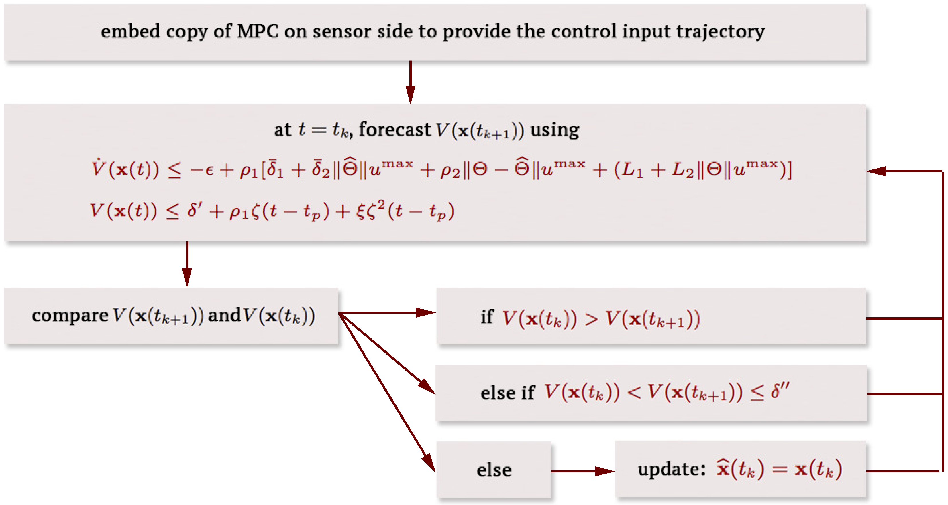
To implement the MPC law of Equation (28), the state measurement must be transmitted to the controller at every sampling time in order to update the model state. To reduce the frequency of sensor–controller information transfer, we proceed in this section to present a forecast-triggered sensor–controller communication strategy that optimizes network resource utilization without compromising closed-loop stability. The basic idea is to forecast at each sampling time the expected evolution (or rate of evolution) of the Lyapunov function over the following sampling interval based on the available state data and the worst-case uncertainty, and to trigger an update of the model state only in the event that the forecast indicates a potential increase in the Lyapunov function or a potential deterioration in the dissipation rate.

To explain how this communication strategy works, we assume that a copy of the MPC law is embedded within the sensors side to provide the control input trajectory and aid the forecasting process. At the same time, the state measurement, $\mathbf{x}$, which is available from the sensors is monitored at the sampling times, and then the model estimation error $\mathbf{e}$ can be computed at each sampling instance. To perform the forecast for $t\in [t_k,t_{k+1})$, the bounds in Equations (36) and (39) are modified as follows:

$$\begin{array}{cc}\hfill \dot{V}\left(\mathbf{x}\left(t\right)\right)\le & -ϵ+{\rho }_1[{\overline{\delta }}_1+{\overline{\delta }}_2\parallel \widehat{\mathsf{\Theta }}\parallel u^{\max }+{\rho }_2\parallel \mathsf{\Theta }-\widehat{\mathsf{\Theta }}\parallel u^{\max }+(L_1+L_2\parallel \mathsf{\Theta }\parallel u^{\max })\zeta (t-t_p)]\hfill \end{array}$$

(40a)

$$\begin{array}{cc}\hfill V\left(\mathbf{x}\right(t\left)\right)\le & {\delta }^{\prime }+{\rho }_1\zeta (t-t_p)+\xi {\zeta }^2(t-t_p)\hfill \end{array}$$

(40b)

where $t_p$ denotes the time that the last update prior to $t_k$ took place. By comparing the above bounds with the original ones developed in Equations (36) and (39) for the case of periodic model updates, it can be seen that the sampling interval, $\tilde{\Delta }$, in the original bounds has now been replaced by the more general interval $t-t_p$. This modification is introduced to allow assessment of the impact of sensor–controller communication suspension on the evolution of the Lyapunov function, and to determine if the suspension could be tolerated for longer than one sampling period.

Algorithm 1 and the flowchart in Figure 1 summarize the proposed forecast-triggered communication strategy. The notation $\overline{V}\left(\mathbf{x}\right)$ is used to denote the upper bound on $V\left(\mathbf{x}\right)$ resulting from the forecast strategy.

Algorithm 1: Forecast-triggered sensor–controller communication strategy

Initialize $\widehat{\mathbf{x}}\left(t_0\right)=\mathbf{x}\left(t_0\right)\in \mathsf{\Omega }$ and set $k=0$, $p=0$

Solve Equation (28) for $[t_0,t_1)$ and implement the first step of the control sequence

if $\widehat{\mathbf{x}}\left(t_{k+1}\right)\in \mathsf{\Omega }\backslash {\mathsf{\Omega }}^{\prime }$ then

Calculate $\overline{V}\left(\mathbf{x}\left(t_{k+2}\right)\right)$ (estimate of $V\left(\mathbf{x}\left(t_{k+2}\right)\right)$) using Equation (40a) and $V\left(\mathbf{x}\left(t_{k+1}\right)\right)$

else

Calculate $\overline{V}\left(\mathbf{x}\left(t_{k+2}\right)\right)$ (estimate of $V\left(\mathbf{x}\left(t_{k+2}\right)\right)$) using Equation (40b) and $\mathbf{e}\left(t_{k+1}\right)$

end if

if $\overline{V}\left(\mathbf{x}\left(t_{k+2}\right)\right)<V\left(\mathbf{x}\left(t_{k+1}\right)\right)$ then

Solve Equation (28) without Equation (28d) for $[t_{k+1},t_{k+2})$

else if $\overline{V}\left(\mathbf{x}\left(t_{k+2}\right)\right)\ge V\left(\mathbf{x}\left(t_{k+1}\right)\right)$ and $\overline{V}\left(\mathbf{x}\left(t_{k+2}\right)\right)\le {\delta }^{\prime }$ then

Solve Equation (28) without Equation (28d) for $[t_{k+1},t_{k+2})$

else

Solve Equation (28) for $[t_{k+1},t_{k+2})$ and set $p=k+1$

end if

Implement the first step of the control sequence on $[t_{k+1},t_{k+2})$

Set $k=k+1$ and go to step 3

Remark 8.

With regard to the implementation of Algorithm 1, the sensors need to obtain measurements of the state $\mathbf{x}$ at each sampling time, $t_k$, perform Steps 3–7 in the algorithm, and then determine whether or not to transmit the state to the controller to update the model state $\widehat{\mathbf{x}}$ based on the criteria described in Steps 8–14. Specifically, once the state arrives at $t=t_{k+1}$, the evolution of $\mathbf{x}\left(t\right)$ over the next sampling interval is forecasted using the actual value of $V\left(\mathbf{x}\left(t_{k+1}\right)\right)$ and $\mathbf{e}\left(t_{k+1}\right)$, as well as the constraint on the Lyapunov function that will become active over the next sampling interval, $[t_{k+1},t_{k+2})$, which is dictated by the location of $\widehat{\mathbf{x}}\left(t_{k+1}\right)$ within Ω relative to ${\mathsf{\Omega }}^{\prime }$. If the projection resulting from the forecast indicates that $\mathbf{x}$ will enter a smaller level set of V or lie within ${\mathsf{\Omega }}^{\prime }$, no update of the model state needs to be performed at $t_{k+1}$ since stability would still be guaranteed over the next sampling interval; otherwise, $\widehat{\mathbf{x}}\left(t_{k+1}\right)$ must be reset to the actual state $\mathbf{x}\left(t_{k+1}\right)$ to suppress the potential instability. Note that the decision to perform or skip a model state update at a given sampling instance is triggered by the prediction of a future event (potential breach of worst-case growth bounds on the Lyapunov function and its time-derivative) instead of a current event (i.e., a simple comparison of the situations at the current and previous sampling instants).

Remark 9.

The condition that $\overline{V}\left(\mathbf{x}\left(t_{k+2}\right)\right)<V\left(\mathbf{x}\left(t_{k+1}\right)\right)$ in Step 8 of Algorithm 1 is used as a criterion for skipping an update at $t_{k+1}$ since satisfying this requirement is sufficient to guarantee closed-loop stability and can also minimize the possibility of performing unnecessary model state updates that merely improve control system performance. When reducing sensor–controller communication is not that critical, or when improved control system performance is an equally important objective, a more stringent requirement on the decay rate of the Lyapunov function can be imposed to help avoid frequent skipping of model state updates and enhance closed-loop performance at the cost of increased sensor–controller communication.

Remark 10.

Notice that the upper bounds used in performing the forecasts of Equation (40) depend explicitly on the magnitude of the fault, Θ, which implies that faults can influence the update rate of the model state and the sensor–controller communication frequency required to attain it. The impact of faults on the sensor–controller communication rate can be mitigated through the use of active fault accommodation and exploiting the dependence of the forecasting bounds on $\widehat{\mathsf{\Theta }}$ which can be used as a fault accommodation parameter and adjusted to help reduce any potential increase in the sensor–controller communication rate caused by the faults. To see how this works, we first note that the term describing the mismatch between Θ and $\widehat{\mathsf{\Theta }}$ in Equation (40a) (i.e., $\parallel \widehat{\mathsf{\Theta }}-\mathsf{\Theta }\parallel$) tends to increase the upper bounds on $\dot{V}$ and V, and therefore cause the projected values of $V\left(\mathbf{x}\right)$ over the next sampling interval to be unnecessarily conservative and large which would trigger more frequent breaches of Step 8 or 10 in Algorithm 1, resulting in increased communication frequency. Actively accommodating the fault by setting $\widehat{\mathsf{\Theta }}=\mathsf{\Theta }$ helps reduce the forecasting bounds and decrease the projected values of V which, in turn, would increase the likelihood of satisfying Step 8 or 10 in Algorithm 1, resulting in the ability to skip more unnecessary update and communication instances. This analysis suggests that, in addition to enhancing closed-loop performance, fault accommodation is desirable in terms of optimizing sensor–controller communication needs (see the simulation example for an illustration of this point). As noted in Remark 6, however, possible errors in estimating the fault magnitude can impact the implementation of this fault accommodation strategy and potentially limit the achievable savings in sensor–controller communication costs.

Remark 11.

The implementation of the forecast-triggered fault-tolerant MPC scheme developed in this work requires the availability of full-state measurements. When only incomplete state measurements are available, an appropriate state estimator with appropriate estimation error convergence properties needs to be designed and incorporated within the control system to provide estimates of the actual states based on the available measurements. The use of state estimates (in lieu of the actual states) in implementing the control and communication policies introduces errors that must be accounted for at the design stage to ensure robustness of the closed-loop system. This can generally be done by appropriately modifying the constraints in the MPC formulation and the communication-triggering thresholds based on the available characterization of the state estimation error. Extension of the proposed MPC framework to tackle the output feedback control problem is the subject of other research work.

6. Simulation Case Study: Application to a Chemical Process

The objective of this section is to demonstrate the implementation of the forecast-triggered fault-tolerant MPC developed earlier using a chemical process example. To this end, we consider a non-isothermal continuous stirred tank reactor (CSTR) with an irreversible first-order exothermic reaction of the form $A\stackrel{k_0}{⟶}B$, where A is the reactant and B is the product. The inlet stream feeds pure A at flow rate F, concentration $C_{A0}$ and temperature $T_{A0}$ into the reactor. The process dynamics are captured by the following set of ordinary differential equations resulting from standard mass and energy balances:

$$\begin{array}{cc}\hfill {\dot{C}}_A& =\frac{F}{V}(C_{A0}-C_A)-k_0\exp \left(\frac{-E}{RT}\right)C_A\hfill \end{array}$$

(41a)

$$\begin{array}{cc}\hfill \dot{T}& =\frac{F}{V}(T_{A0}-T)-\frac{\Delta H}{\rho c_p}{k}_0\exp \left(\frac{-E}{RT}\right)C_A+\frac{Q}{\rho c_{p}V}\hfill \end{array}$$

(41b)

where $C_A$ is the concentration of A in the reactor; T is the reactor temperature; V is the reactor volume; $k_0$, E, and $\Delta H$ represent the pre-exponential factor, the activation energy, and the heat of reaction, respectively; R denotes the ideal gas constant; $c_p$ and $\rho$ are the heat capacity and density of the fluid in the reactor, respectively; and Q is the rate of heat transfer from the jacket to the reactor. The process parameter values are given in

Table 1. Process and model parameter values for the continuous stirred tank reactor (CSTR) example in Equation (41).

Parameter	Process	Model
F (m3/h)	$3.34\times {10}^{-3}$	$3.34\times {10}^{-3}$
V (m3)	$0.1$	$0.1$
$k_0$ (h−1)	$1.2\times {10}^9$	$1.2\times {10}^9$
E (KJ/Kmol)	$8.314\times {10}^4$	$8.30\times {10}^4$
R (KJ/Kmol/K)	$8.314$	$8.314$
$\rho$ (Kg/m3)	1000	1010
$C_p$ (KJ/Kg/K)	$0.239$	$0.24$
$\Delta H$ (KJ/Kmol)	$-4.78\times {10}^4$	$-4.8\times {10}^4$
$C_{A0}^s$ (Kmol/m3)	$0.79$	$0.79$
$T_0^s$ (K)	$352.6$	$352.6$
$Q^s$ (KJ/h)	0	0

.

The control objective is to stabilize the process state near the open-loop unstable steady-state ($C_A^s=0.577$ Kmol/m³, $T^s=395.3$ K) in the presence of input constraints, control actuator faults and limited sensor–controller communication. The manipulated input is chosen as the inlet reactant concentration, i.e., $\mathbf{u}=C_{A0}-C_{A0}^s$, subject to the constraint $\parallel \mathbf{u}\parallel \le 0.5\mathrm{mol}/{\mathrm{m}}^3$, where $C_{A0}^s$ is the nominal steady state value of $C_{A0}$, and control actuator faults. We define the displacement variables $\mathbf{x}={\left[x_1{x}_2\right]}^T={[C_A-C_A^{s}T-T^s]}^T$, where the superscript s denotes the steady state value, which places the nominal equilibrium point of the system at the origin. A quadratic Lyapunov function candidate of the form $V\left(\mathbf{x}\right)={\mathbf{x}}^T\mathbf{P}\mathbf{x}$, where:

$$\mathbf{P}=\left[\begin{array}{cc}\mathrm{37,400}& 1394.9\\ 1394.9& 63.5389\end{array}\right]$$

(42)

is a positive-definite matrix, is used for the synthesis of the controller in Equation (5) and the characterization of the closed-loop stability region in Equations (8) and (9). The value of the tuning parameter $\lambda$ is fixed at 0.1 to ensure an adequate margin of robustness while providing an acceptable estimate of the stability region.

6.1. Characterization of the Fault-Tolerant Stabilization Region

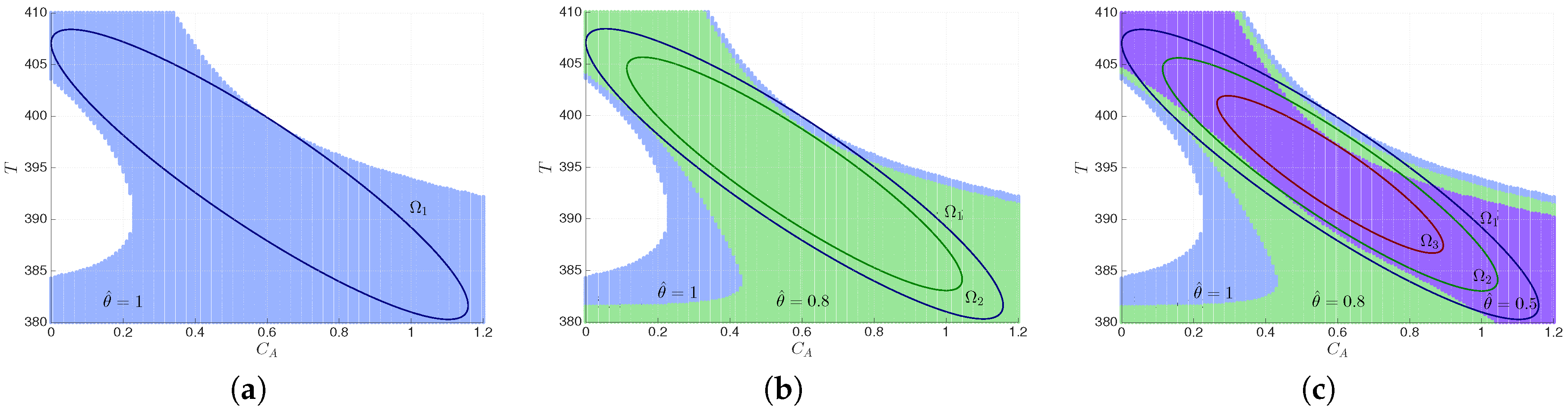
Recall from Section 4 that the MPC formulation in Equation (28) inherits its closed-loop stability region from the auxiliary bounded controller, and that this region is explicitly dependent on the magnitude of the fault (see Equations (8) and (9)). Figure 2 depicts the dependence of the constrained stability region on fault severity. Specifically, the blue region refers to $\mathsf{\Psi }\left(u^{\max }\right|\widehat{\theta }=1)$, i.e., when the actuator is perfectly healthy; while the green and purple regions represent $\mathsf{\Psi }\left(u^{\max }\right)$ when $\widehat{\theta }=0.8$, and $\widehat{\theta }=0.5$, respectively. As all three regions are projected on a single plot, the purple region is completely contained within the green region which is fully contained within the blue region, i.e., $\mathsf{\Psi }\left(u^{\max }\right|\widehat{\theta }=0.5)\subset \mathsf{\Psi }\left(u^{\max }\right|\widehat{\theta }=0.8)\subset \mathsf{\Psi }\left(u^{\max }\right|\widehat{\theta }=1)$. The largest level set $\mathsf{\Omega }$ within each region $\mathsf{\Psi }\left(u^{\max }\right)$ is represented by the ellipse with the corresponding darker color. The three level sets form concentric ellipses and follow the same trend with $\mathsf{\Omega }\left(u^{\max }\right|\widehat{\theta }=0.5)\subset \mathsf{\Omega }\left(u^{\max }\right|\widehat{\theta }=0.8)\subset \mathsf{\Omega }\left(u^{\max }\right|\widehat{\theta }=1)$. Figure 2 shows that the stability region shrinks in size as $\widehat{\theta }$ decreases and the severity of the fault increases. Each level set in this figure provides an estimate of the set of initial states starting from which closed-loop stability is guaranteed in the presence of the corresponding fault.

6.2. Active Fault Accommodation in the Implementation of MPC

As discussed in Section 3 and Section 4, the presence of control actuator faults generally reduces the stability region of the closed-loop system and enlarges the terminal set, which potentially compromises the stability and performance properties of the closed-loop system. The implementation of active fault accommodation measures such as adjusting the value of $\widehat{\mathsf{\Theta }}$ in the model, however, can help reduce the mismatch between the fault and its estimate used by the MPC, and therefore help reduce the size of the terminal set which can improves the closed-loop steady state performance. In this section, the MPC introduced in Equation (28) is implemented using the model parameters reported in Table 1 with an optimization horizon of 20 s and a sampling period of 2 s. The nonlinear optimization problem is solved using the standard “fmincon” algorithm in Matlab which generally yields locally optimal solutions. A step fault of $\theta =0.8$ is introduced in the actuator at $t=50$ s and persists thereafter.

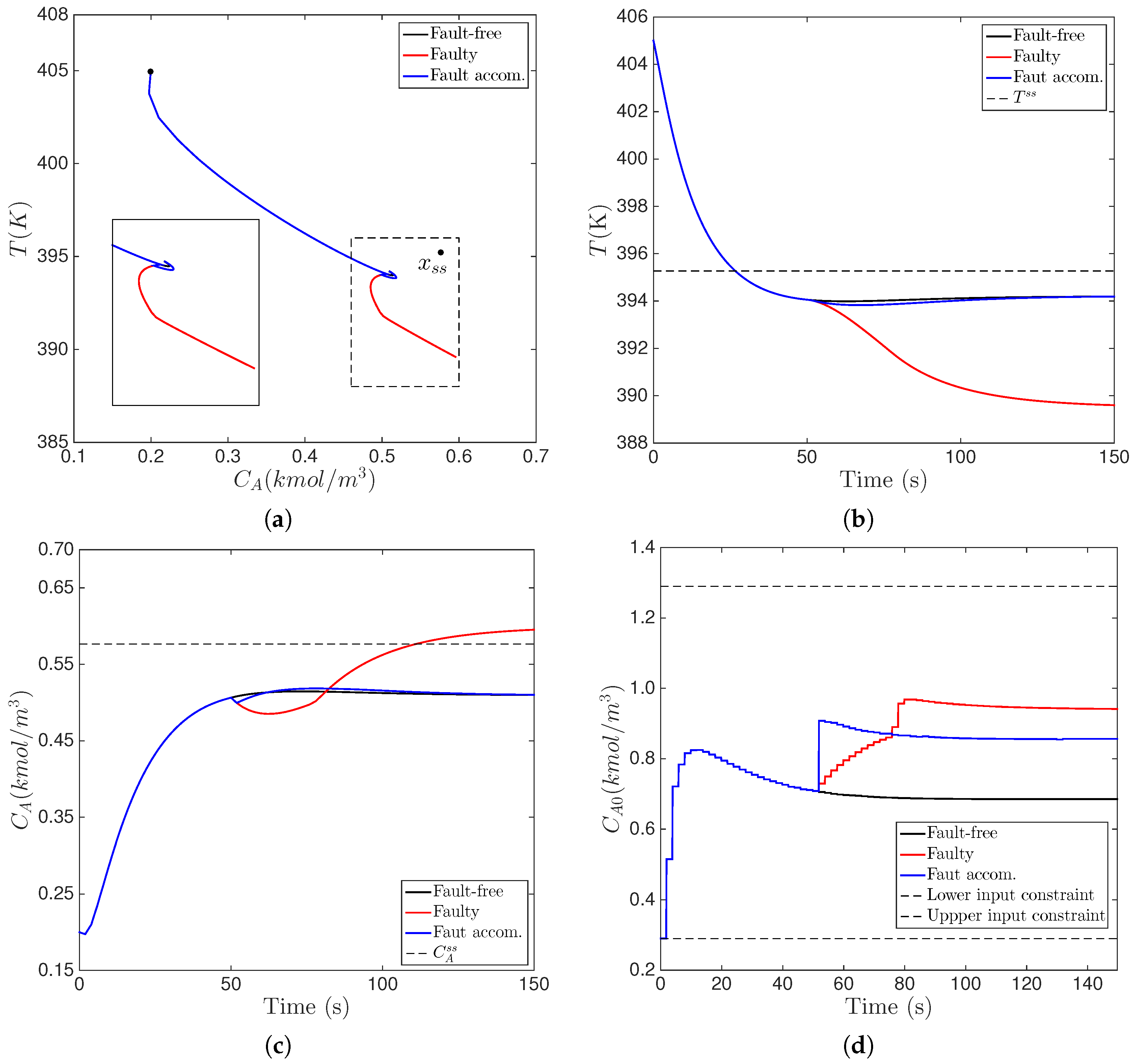
Figure 3 compares the performance of the closed-loop system in the absence of faults (fault-free operation scenario in black) with the performance of the closed-loop system in the presence of faults (blue and red). The blue profiles depict the performance when the fault is accommodated, while the red profiles illustrate the performance when the fault is left unaccommodated. The dashed lines in Figure 3b,c represent the target steady-state values for the reactor temperature and reactant concentration, respectively. A steady-state offset resulting from the effect of discrete measurement sampling can be observed in Figure 3a–c, which indicates that with the uncertain model used, when the MPC is implemented in a sample-and-hold fashion, only ultimate boundedness can be achieved. The red profiles show that the fault pushes the closed-loop state trajectory away from the desired steady state and increases the size of the terminal set significantly. However, when accommodated by setting $\widehat{\theta }=\theta =0.8$ upon detection of the fault, a performance comparable to that obtained in the fault-free operation scenario can be achieved, as the blue profiles are very close to the black profiles in Figure 3a–c.

6.3. Implementation of Fault-Tolerant MPC Using Forecast-Triggered Sensor–Controller Communication

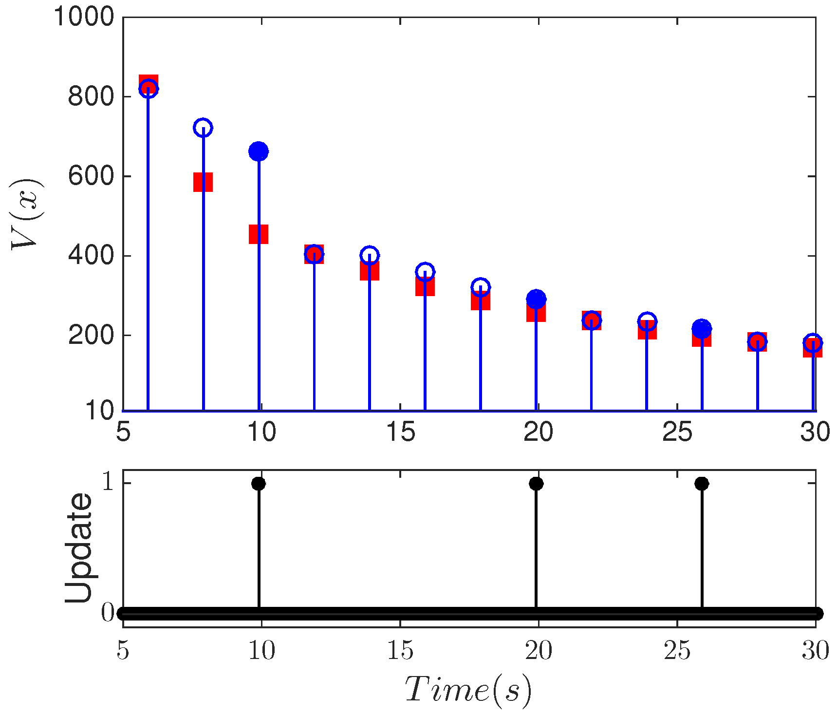
In this section, we illustrate the forecast-triggered implementation strategy of MPC and highlight the resulting reduction in network resource utilization. To this end, we consider first the case of fault-free operation. Figure 4 illustrates the implementation of Algorithm 1. Each red square in the top plot represents the current value of $V\left(\mathbf{x}\right)$ at the corresponding sampling instant $t_k$, and each blue circle represents the forecasted value of $V\left(\mathbf{x}\right)$ calculated one sampling interval ahead. An update of the model state is triggered at a given sampling time $t_k$ if either: (1) the forecasted $V\left(\mathbf{x}\left(t_{k+1}\right)\right)$ is greater than the current $V\left(\mathbf{x}\left(t_k\right)\right)$ (whenever $V\left(\mathbf{x}\left(t_k\right)\right)>{\delta }^{\prime }$), or (2) $V\left(\mathbf{x}\left(t_k\right)\right)<{\delta }^{\prime }<V\left(\mathbf{x}\left(t_{k+1}\right)\right)$. The model state update events are depicted by the solid blue dots in the plot. The update profile shown in the bottom panel indicates the times when the model state updates take place. In this plot, a value of 1 denotes that an update event has occurred, while a value of zero indicates that an update has been skipped. Figure 4 captures only the case when $V\left(\mathbf{x}\left(t_k\right)\right)>{\delta }^{\prime }$ (i.e., when the closed-loop trajectory lies outside the terminal set).

By examining Figure 4, it can be seen that at $t=8$ s (the 4th sampling time), $V\left(\mathbf{x}\left(t_4\right)\right)=586$ which is represented by the red square, and that $\overline{V}\left(\mathbf{x}\left(t_5\right)\right)$ is forecasted to exceed the current value, which is represented by the blue dot at $t=10$ s, which means that, without resetting the model state at $t=8$ s, it is possible for $V\left(\mathbf{x}\right(t\left)\right)$ to start to grow over the next sampling interval. To prevent the potential destabilizing tendency, a model state update is performed at $t=8$ s as shown in the update profile at the bottom of the plot. Similarly, model state updates are triggered at $t=20$ s and $t=26$ s as a result of implementing the forecast-triggered communication strategy. At the other sampling instants, the condition of $V\left(\mathbf{x}\left(t_{k+1}\right)\right)\le V\left(\mathbf{x}\left(t_k\right)\right)$ is satisfied and model state updates are not triggered.

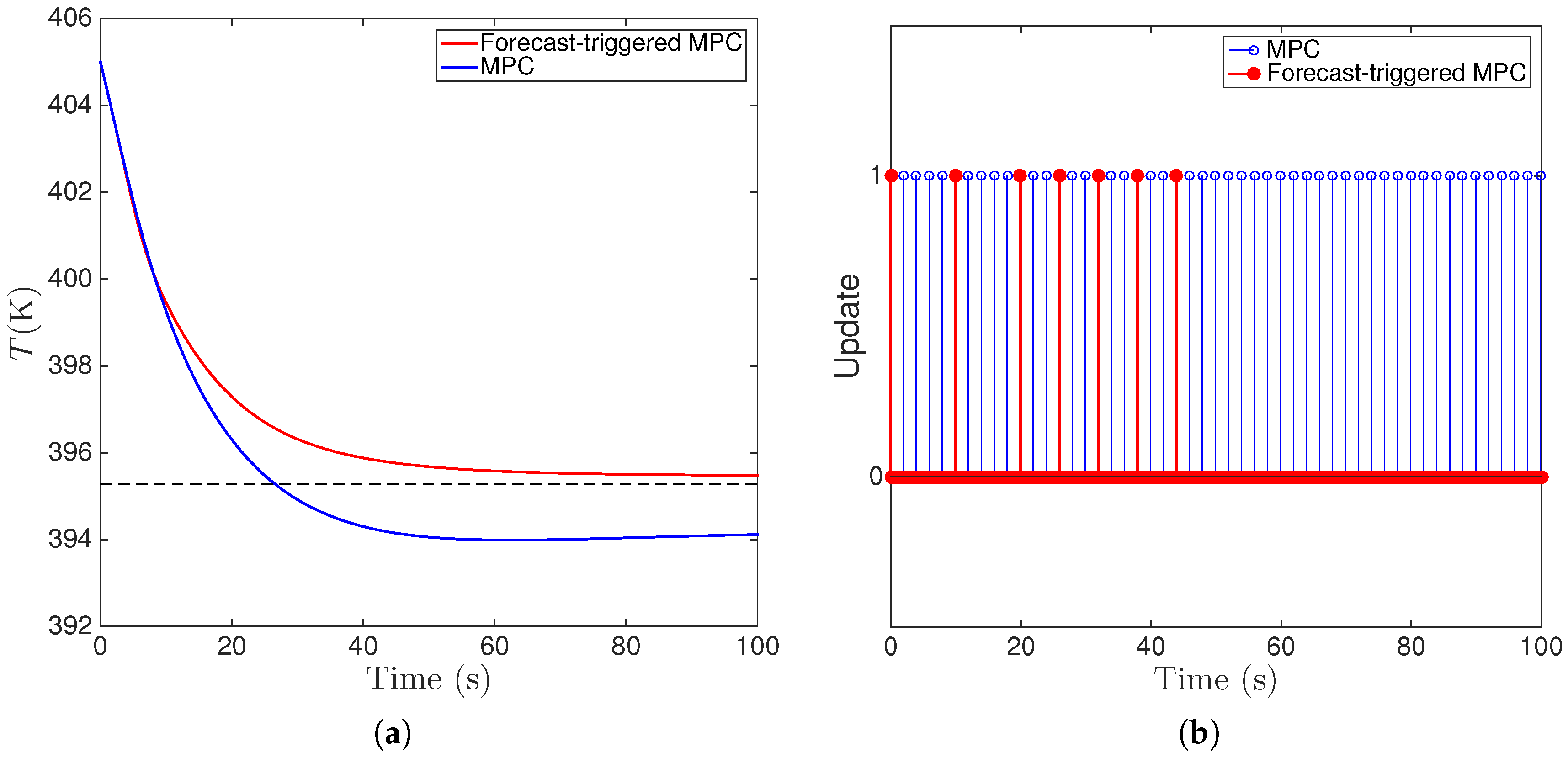
The resulting closed-loop behavior is depicted by the red profile in Figure 5a which shows that the forecast-triggered communication strategy successfully stabilizes the reactor temperature near the desired steady state. Figure 5b compares the number of model state updates under a conventional MPC (where an update is performed at each sampling time) and the forecast-triggered MPC (where an update is performed only when triggered by a breach of the stability threshold). The comparison shows that stabilization using the forecast-triggered MPC requires only 14% of the model state updates over the same time interval, and is thus achieved with a significant reduction in the sensor–controller communication frequency.

An examination of Figure 5a shows that the conventional MPC slightly outperforms the forecast-triggered MPC initially (i.e., during the transient stage) in the sense that it enforces a faster and more aggressive convergence of the closed-loop state. This is expected given the more frequent model state updates performed by the conventional MPC. It is interesting to note though that the forecast-triggered MPC exhibits a much smaller steady state offset (i.e., a smaller terminal set) despite the less frequent sensor–controller communication in this case. It should be noted, however, that the larger steady state offset achieved by the conventional MPC is not an indication of poorer performance, but is rather due to the different ways in which the two MPC schemes were implemented and the fact that for the event-triggered MPC a desired terminal set was specified a priori as part of the controller design and implementation logic, whereas for the conventional MPC a desired terminal set size was not specified. Specifically, for the forecast-triggered MPC, a small terminal set size was initially specified and then the sensor–controller communication logic was designed and implemented to keep the closed-loop state trajectory within that terminal set. For the conventional MPC, however, no specification of the desired terminal set was enforced. While it is possible, in principle, to specify the same terminal set for both MPC schemes, it was found that excessively fast sampling would be required to enforce the same tight convergence for the conventional MPC.

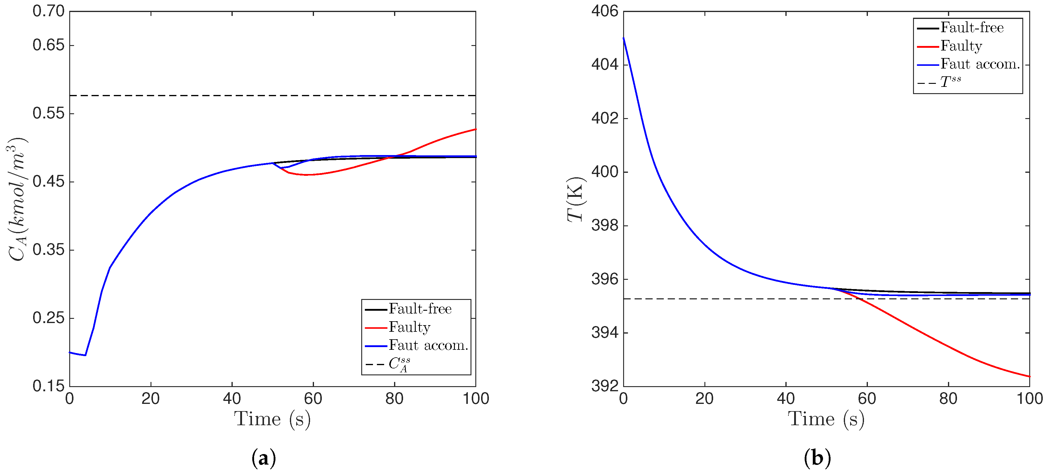
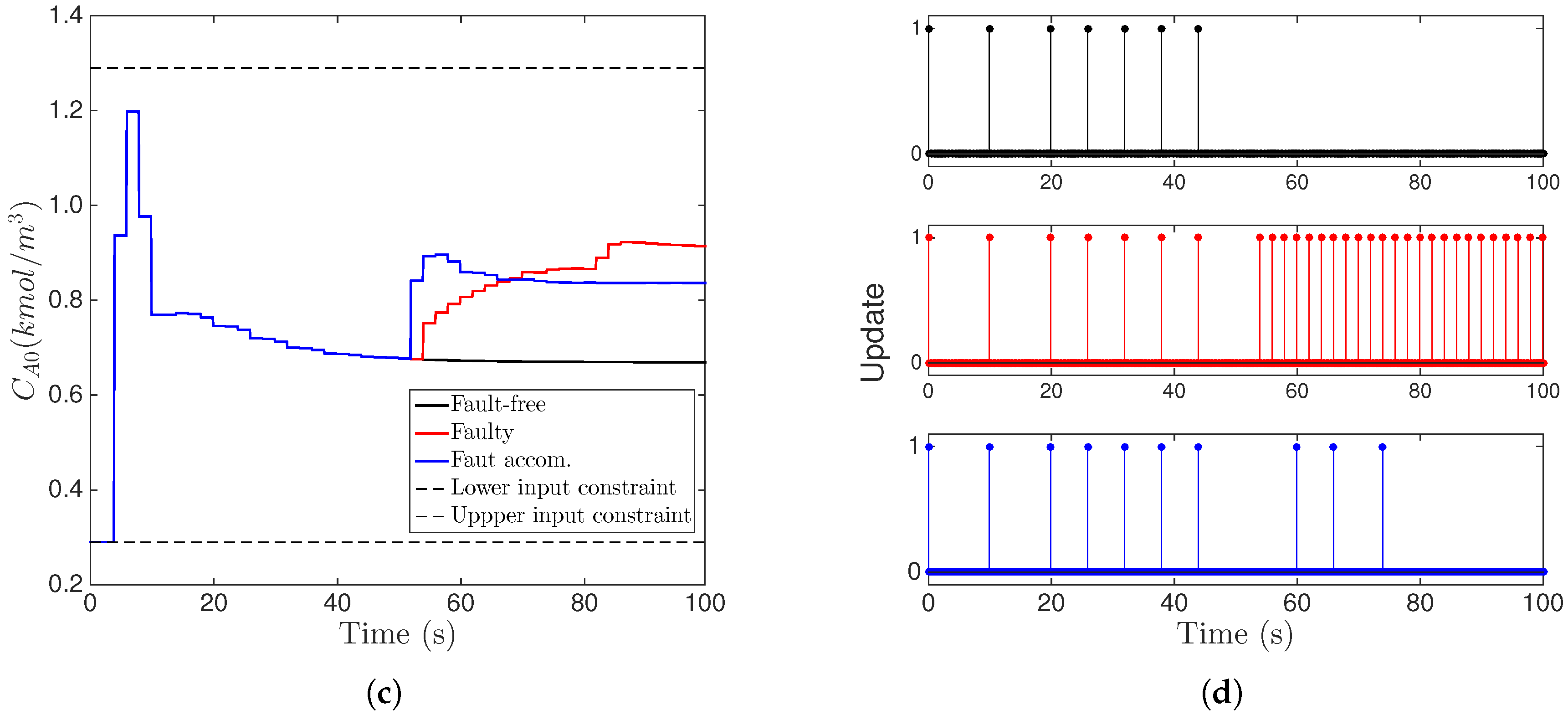
To demonstrate the benefits of active fault accommodation in the context of the forecast-triggered MPC scheme, we now consider the same fault scenario introduced earlier, where $\theta \left(t\right)=0.8$ for $t\ge 50$ s. Figure 6 compares the performance of the closed-loop system in the fault-free scenario (shown in black) with those in the faulty operation cases, including the case when the actuator fault is accommodated (shown in blue) and the case when the actuator fault is left unaccommodated (shown in red). Similar to the result obtained in Figure 3, fault accommodation (realized by setting $\widehat{\theta }=\theta =0.8$ at $t=50$ s) reduces the steady-state offset and achieves closed-loop state profiles comparable to those obtained in the fault-free scenario. Figure 6d shows the corresponding model state update frequencies for the three cases. Recall that faults not only influence the closed-loop state performance, but can also negatively impact the projected bounds on the Lyapunov function or its derivative which are used in the forecasting strategy that triggers the model state updates. It can be seen from the middle plot in Figure 6d that when the fault is left unaccommodated an update of the model state is triggered at every sampling time after $t=50$ s. In contrast, when the fault is appropriately accommodated, only three model state updates are needed after $t=50$ s (see the bottom plot in Figure 6d) which yields an improved closed-loop performance. These results illustrate that the proposed fault accommodation strategy is beneficial for both performance improvement as well as network load reduction.

7. Conclusions

In this paper, a forecast-triggered fault-tolerant Lyapunonv-based MPC scheme is developed for constrained nonlinear systems with sensor–controller communication constraints. An auxiliary fault-tolerant bounded controller is initially designed to aid in the characterization of the region of fault-tolerant stabilization and subsequent design of the Lyapunov-based MPC. To handle sensor–controller communication constraints in the networked control system design, a forecast-triggered strategy for managing the sensor–controller information transfer is developed. In this strategy, model state updates using actual state measurements are triggered only when certain stability thresholds—derived based on a worst-case projection of the state trajectory—are breached. A simulation case study is presented to illustrate the implementation of the proposed MPC and its fault accommodation capabilities. The results show that the proposed design is effective in achieving closed-loop stability while simultaneously reducing communication network load.

References

- Qin, S.J.; Badgwell, T.A. A survey of industrial model predictive control technology. Control Eng. Pract. 2003, 11, 733–764. [Google Scholar] [CrossRef] [Green Version]
- Rawlings, J.B.; Mayne, D.Q. Model Predictive Control: Theory and Design; Nob Hill Publishing: Madison, WI, USA, 2009. [Google Scholar]
- Christofides, P.D.; Liu, J.; de la Pena, D.M. Networked and Distributed Predictive Control: Methods and Nonlinear Process Network Applications; Springer: London, UK, 2011. [Google Scholar]
- Ellis, M.; Liu, J.; Christofides, P.D. Economic Model Predictive Control: Theory, Formulations and Chemical Process Applications; Springer: London, UK, 2017. [Google Scholar]
- Blanke, M.; Kinnaert, M.; Lunze, J.; Staroswiecki, M. Diagnosis and Fault-Tolerant Control; Springer: Berlin/Heidelberg, Germany, 2003. [Google Scholar]
- Zhang, Y.; Jiang, J. Bibliographical Review on Reconfigurable Fault-Tolerant Control Systems. Annu. Rev. Control 2008, 32, 229–252. [Google Scholar] [CrossRef]
- Mhaskar, P.; Liu, J.; Christofides, P.D. Fault-Tolerant Process Control: Methods and Applications; Springer: London, UK, 2013. [Google Scholar]
- Christofides, P.D.; Davis, J.; El-Farra, N.H.; Clark, D.; Harris, K.; Gipson, J. Smart plant operations: Vision, progress and challenges. AIChE J. 2007, 53, 2734–2741. [Google Scholar] [CrossRef]
- Mhaskar, P. Robust Model Predictive Control Design for Fault-Tolerant Control of Process Systems. Ind. Eng. Chem. Res. 2006, 45, 8565–8574. [Google Scholar] [CrossRef]
- Dong, J.; Verhaegen, M.; Holweg, E. Closed-loop subspace predictive control for fault-tolerant MPC design. In Proceedings of the 17th IFAC World Congress, Seoul, Korea, 6–11 July 2008; pp. 3216–3221. [Google Scholar]
- Camacho, E.F.; Alamo, T.; de la Pena, D.M. Fault-tolerant model predictive control. In Proceedings of the IEEE Conference on Emerging Technologies and Factory Automation, Bilbao, Spain, 13–16 September 2010; pp. 1–8. [Google Scholar]
- Lao, L.; Ellis, M.; Christofides, P.D. Proactive Fault-Tolerant Model Predictive Control. AIChE J. 2013, 59, 2810–2820. [Google Scholar] [CrossRef]
- Knudsen, B.R. Proactive Actuator Fault-Tolerance in Economic MPC for Nonlinear Process Plants. In Proceedings of the 11th IFAC Symposium on Dynamics and Control of Process Systems, Trondheim, Norway, 6–8 June 2016; pp. 1097–1102. [Google Scholar]
- Hu, Y.; El-Farra, N.H. Quasi-decentralized output feedback model predictive control of networked process systems with forecast-triggered communication. In Proceedings of the American Control Conference, Washington, DC, USA, 17–19 June 2013; pp. 2612–2617. [Google Scholar]
- Hu, Y.; El-Farra, N.H. Adaptive quasi-decentralized MPC of networked process systems. In Distributed Model Predictive Control Made Easy; Springer: Dordrecht, The Netherlands, 2014; Volume 69, pp. 209–223. [Google Scholar]
- Christofides, P.D.; El-Farra, N.H. Control of Nonlinear and Hybrid Process Systems: Designs for Uncertainty, Constraints and Time-Delays; Springer: Berlin, Germany, 2005. [Google Scholar]
- Mhaskar, P.; El-Farra, N.H.; Christofides, P.D. Stabilization of Nonlinear Systems with State and Control Constraints Using Lyapunov-Based Predictive Control. Syst. Control Lett. 2006, 55, 650–659. [Google Scholar] [CrossRef]
- Allen, J.; El-Farra, N.H. A Model-based Framework for Fault Estimation and Accommodation Applied to Distributed Energy Resources. Renew. Energy 2017, 100, 35–43. [Google Scholar] [CrossRef]
- Sanchez-Sanchez, K.B.; Ricardez-Sandoval, L.A. Simultaneous Design and Control under Uncertainty Using Model Predictive Control. Ind. Eng. Chem. Res. 2013, 52, 4815–4833. [Google Scholar] [CrossRef]
- Bahakim, S.S.; Ricardez-Sandoval, L.A. Simultaneous design and MPC-based control for dynamic systems under uncertainty: A stochastic approach. Comput. Chem. Eng. 2014, 63, 66–81. [Google Scholar] [CrossRef]
- Gutierrez, G.; Ricardez-Sandoval, L.A.; Budman, H.; Prada, C. An MPC-based control structure selection approach for simultaneous process and control design. Comput. Chem. Eng. 2014, 70, 11–21. [Google Scholar] [CrossRef]
Figure 1.
Flowchart of implementation of the forecast-triggered communication strategy. MPC: model predictive control.
Figure 2.
Estimates of the region of guaranteed fault-tolerant stabilization under MPC: (a) represents the estimate when (blue level set); (b) represents the estimate when (green level set); (c) represents the estimate when (purple level set).
Figure 3.
Comparison of the evolutions of: (a) the closed-loop state trajectory; (b) the closed-loop reactor temperature T; (c) the closed-loop reactant concentration ; and (d) the manipulated input, , for three different operating scenarios: one in the absence of any faults (black profiles); one in the presence of a fault but without implementing any fault accommodation (red profiles); and one in the presence of a fault and implementing fault accommodation (blue profiles).
Figure 4.
Illustration of how the forecast-triggered sensor–controller communication strategy is implemented. The top plot depicts current values of the Lyapunov function (red squares), projected values of the Lyapunov function (blue circles) and update events (solid blue dots) at different sampling times. The bottom plot depicts the time instances when the model state is updated.
Figure 5.
Closed-loop reactor temperature profiles (a); and model state update instances (b) under the conventional (blue) and forecast-triggered MPC schemes (red).
Figure 6.
Comparison of the performance of forecast-triggered MPC scheme under fault-free conditions (black), an accommodated fault scenario (blue) and an unaccommodated fault scenario (red): (a) closed-loop temperature profiles; (b) reactant concentration profiles; (c): manipulated input profile; and (d): model update frequency.