A New Radial Basis Function Approach Based on Hermite Expansion with Respect to the Shape Parameter


Department of Mechanical and Manufacturing Engineering, University of Calgary, 2500 University Drive NW, Calgary, AB T2N 1N4, Canada
*
Author to whom correspondence should be addressed.
Mathematics 2019, 7(10), 979; https://0-doi-org.brum.beds.ac.uk/10.3390/math7100979
Submission received: 18 August 2019
/
Revised: 12 October 2019
/
Accepted: 14 October 2019
/
Published: 16 October 2019
Abstract
:Owing to its high accuracy, the radial basis function (RBF) is gaining popularity in function interpolation and for solving partial differential equations (PDEs). The implementation of RBF methods is independent of the locations of the points and the dimensionality of the problems. However, the stability and accuracy of RBF methods depend significantly on the shape parameter, which is mainly affected by the basis function and the node distribution. If the shape parameter has a small value, then the RBF becomes accurate but unstable. Several approaches have been proposed in the literature to overcome the instability issue. Changing or expanding the radial basis function is one of the most commonly used approaches because it addresses the stability problem directly. However, the main issue with most of those approaches is that they require the optimization of additional parameters, such as the truncation order of the expansion, to obtain the desired accuracy. In this work, the Hermite polynomial is used to expand the RBF with respect to the shape parameter to determine a stable basis, even when the shape parameter approaches zero, and the approach does not require the optimization of any parameters. Furthermore, the Hermite polynomial properties enable the RBF to be evaluated stably even when the shape parameter equals zero. The proposed approach was benchmarked to test its reliability, and the obtained results indicate that the accuracy is independent of or weakly dependent on the shape parameter. However, the convergence depends on the order of the truncation of the expansion. Additionally, it is observed that the new approach improves accuracy and yields the accurate interpolation, derivative approximation, and PDE solution.
1. Introduction
During the past few decades, radial basis function (RBF)-based methods have attracted researchers’ attention as methods for interpolation and solving partial differential equations (PDEs). These methods are popular due to their simplicity and high convergence rate. However, this convergence rate depends on the shape parameter of the RBF. Numerous approaches have been followed in the literature to address this problem.Hermite interpolation techniques and Hermite orthogonal polynomials are among the approaches that can be applied to RBF methods. In general, Hermite techniques can be applied to RBF methods through either of two approaches. The first one is based on the application of the Hermite interpolation technique, which changes the interpolant to incorporate the function derivative or the PDE operator in addition to the basis function. The second approach is based on the projection of the RBF on the Hermite polynomial space. These techniques are reviewed and considered in this work because they are closely related to the present contribution.
1.1. Changing the Interpolant
Radial basis function methods are used to obtain an accurate grid-free approximation of a function with a strong gradient [1]. Kansa [2] used an RBF to solve PDEs by direct collocation. Fasshauer [3] changed the interpolant by using Hermite interpolation to improve the condition number of the matrix of the differential operator of PDE. This matrix is symmetric, which reduces the amount of computation, particularly for large matrices. Compared with Kansa’s approach, Fasshauer’s approach requires a higher derivative of the basis function to evaluate the same differential operator, hence, Kansa’s approach is simpler. The convergence of Fasshauer’s approach was verified and compared with the theoretical one [4]. The compactly supported RBF was used with Fasshauer’s method to enhance the accuracy near the boundary [5]. Kansa’s and Fasshauer’s approaches have been compared in the literature to solve the steady-state convection–diffusion equation at high Peclet number values [6]. The comparison results reveal that both approaches are more convenient to implement than conventional methods, such as the finite difference, finite element, and finite volume. It was also observed that, for steady-state problems, Fasshauer’s approach was marginally better than Kansa’s because it did not require an artificial damping term. Another comparison between Kansa’s and Fasshauer’s approaches was conducted by Fasshauer [7] to solve time-dependent and time-independent PDEs. It was observed that Kansa’s approach generated an invertible interpolation matrix. Hence, the discrete differential operator could always be formed, rendering this approach more suitable for time-dependent PDEs. Furthermore, Fasshauer’s approach generated a symmetric and invertible PDE matrix and a poor conditioned interpolation matrix. Consequently, it was not possible to stably calculate the discrete differential operator, which made Fasshauer’s approach more suitable for time-independent PDEs. Rocca et al. [8] proposed the use of the Crank–Nicholson method for discretizing the temporal term in a time-dependent PDE to perceive time-dependent PDEs as a time-independent PDE with an additional term related to the solution of the previous time-step. As a result, the time-dependent PDEs could be solved stably with Fasshauer’s approach. RBF-FD was used with Fasshauer’s approach [9] to improve the accuracy by applying a small local stencil of nodes. This approach was enhanced by using a variable shape parameter based on the root-mean-square (RMS) error [10] to predict the optimal shape parameter value that minimizes the error. Rocca et al. [11] extended Fasshauer’s method by applying the differential operator to the boundary, in addition to the interpolation operator. This approach satisfied both the PDEs and the function at and near the boundary. Rocca’s approach improved the accuracy of the RBF at the boundary. By considering different locations for interpolation and PDE points, Stevens et al. [12] extended Fasshauer’s method to enhance the results of PDEs with high Peclet numbers. In contrast to Fasshauer’s method, Stevens et al.’s approach applied the interpolation operator to the interpolation points and padded them to the matrix resulting from Fasshauer’s method. It should be noted that Stevens et al.’s approach is applicable only to time-independent PDEs or to time-dependent PDEs using the modification proposed in [8]. Fasshauer’s approach and its derivatives have been used successfully for a wide range of applications in the literature. For example, they have been used for simulating cooling and freezing [13], nonlinear heat equations [14,15], and nonlinear convection–diffusion equations [16]. From these previous contributions, it can be concluded that applying the Hermite collocation technique to an RBF improves the accuracy by varying the approximant, however, it does not improve the stability when the shape parameter approaches zero. Recently, researchers have shifted their attention to changing the basis for improved stability.
1.2. Changing the Basis
Changing the basis of RBFs has been attempted several times in the past few decades to improve accuracy and stability when the shape parameter is approaching zero [17,18,19,20,21,22,23,24,25,26,27,28,29,30]. Recently, researchers have used the Hermite expansion of the radial basis function because it enjoys the recursive relation and orthogonality. For example, Rashidinia et al. [20] enhanced the eigenfunction expansion (Mercer’s theorem) of a positive definite function by using the Hermite expansion with respect to scaled distances (r), this enabled the construction of a new stable basis. Due to the orthogonality of the eigenfunctions and Hermite expansion, it is possible to form the discrete differential operator without inverting the interpolation matrix. It is observed that instability can arise from sources other than small shape parameter values. This stable basis can also be unstable for a large truncation order of the Hermite polynomial; this necessitates the use of higher-precision calculations in certain cases. Notwithstanding the previous advantages, the approach of Rashidinia et al. [20] is effective only on tensor-product meshes for higher-dimension problems. Yurova et al. [21] proposed another algorithm based on Hermite polynomials to stabilize the RBF method when the shape parameter approaches zero. Yurova et al.’s algorithm does not require a complex selection of parameters and provides a simpler extension to high-dimensional tensor-product meshes. The previously mentioned approaches have relatively complex parameters and operate effectively only on tensor-product meshes for higher-dimension problems. These drawbacks motivated us to improve the basis of the RBF method further.
1.3. Current Work
The literature shows that for small values of the shape parameter, the RBF becomes unstable. In this work, the Hermite orthogonal polynomial is used to expand the RBF basis with respect to shape parameter in order to determine a stable basis and to stably evaluate the RBF at and near the zero shape parameter. The present approach could be used on arbitrary mesh points, even for a higher dimension, without the constraint of having to use tensor-product meshes.
The rest of this article is organized as follows. Section 2 explains how RBFs are used for approximating derivatives and solving PDEs with Kansa’a and Fasshauer’s approaches. In Section 3, the application of the Hermite polynomial on the RBF basis with respect to the shape parameter is described. The results are presented in the fourth section. Finally, the conclusions and future works are discussed.
2. The Radial Basis Function Method
As mentioned in the introduction, the approximant of the RBF method can be expressed in a number of ways. For simplicity, Kansa’s and Fasshauer’s approximants are presented and discussed. Assume that represents points that belong to a set of points of a bounded domain . can be divided into a set of interior points I and a set of boundary points B located on the domain boundary (). For the interpolation of a specified data point at locations, the approximant should be defined. Then, the interpolation can be used to solve time-dependent PDEs on . For example, the following PDE form is considered:
where and g are the linear differential operator and the boundary values, respectively. The aim is to express this partial differential equation in terms of an RBF (); here, is the shape parameter, and is the distance between two points in space. It is convenient to define a convention to specify which differential operator or function is applied to which group of points of the domain from and among internal points (I), boundary points (B), and all points (). For example, is a matrix that contains the differential operator applied to and evaluated at ; here, and . Similarly, is a vector consisting of ; here, . This convention is used in the subsequent two subsections to describe Kansa’s and Fasshauer’s approaches to solve the PDE.
2.1. Kansa’s Approach
Kansa’s approach has been widely used in the literature because it is simple and convenient to implement. Moreover, it does not incorporate the derivative of the basis or the differential operator in the approximant. It expresses the approximant () in terms of the radial basis function without modification:
where denotes coefficients associated with each basis, they can be determined by imposing the interpolation constraints on the approximant. This can be achieved by equating the approximant at points to the specified data at the same location ().
Equation (4) is a linear system of equations that can be expressed in a matrix format:
The matrix is a symmetric and invertible matrix if no repeated point is used. This property is effective when solving PDEs because it reduces the computational cost. The differential operator can be applied to the approximant at the interior points to solve the PDE (Equation (2)).
Two approaches can be followed to proceed. The first involves the calculation of the coefficients at each time-step from Equation (5) by inverting the matrix . This approach is computationally expensive. However, the computational cost of the calculation can be reduced by utilizing the symmetry of the matrix. Then, the coefficients are substituted in Equation (6) to approximate the differential operator. Although this approach exhibits higher accuracy, it is not preferable for solving PDEs because it incurs a high computational cost. In the second approach, the coefficients are calculated analytically from Equation (5) by inverting the matrix . The solution is substituted in Equation (6):
The discrete differential operator (W) can be formed without explicitly calculating the coefficients. The calculation needs to be carried out once before starting the time iteration. Then, the discrete differential operator (W) can be used at each time-step to obtain the solution of the partial differential equation.
2.2. Fasshauer’s Approach
Fasshauer’s approach is based on changing the approximant to obtain a symmetric PDE matrix. This can be achieved by applying different operators for a different group of nodes. For example, the approximant for the specified PDE can be expressed as follows:
The differential operator is equivalent to , however, it is applied to the second independent variable of r (i.e., ) rather than the first (). The interpolation constraints should be imposed on the approximant to determine the interpolation coefficients, this can be achieved by equating the approximant at points to .
Equation (9) is a system of equations, it can be represented using matrices:
Similar to Kansa’s approach, the coefficients and can be calculated from the interpolation matrix, although the interpolation matrix is not symmetric. It is necessary to form the PDE matrix by applying the differential operator to the interior points in order to solve the PDE:
The coefficients can be obtained by solving the interpolation system of equations (Equation (10)). Then, they are substituted in Equation (11) to obtain the discrete differential operator (W):
2.3. Time Integration
The temporal term in the PDE is essential and should be addressed with caution when solving PDEs. As previously established, the RBF function can generate a higher-order discretization of space. Hence, it is necessary to use higher-order time discretization to achieve reasonable accuracy and stability. This explains the reason that the implicit time discretization proposed in [8] is rolled out from this study. Runge–Kutta time discretization is used because it exhibits higher accuracy than both the explicit first-order Euler method and the implicit second-order method. Prior to applying the Runge–Kutta method, the equations resulting from Kansa’s and Fasshauer’s approaches should be unified. Both Kansa’s and Fasshauer’s formulations for solving PDE can be expressed as
The explicit fourth-order Runge–Kutta method is used to discretize Equation (13) in time
where is the new value of f at the subsequent time-step.
In this section, it is illustrated that the interpolation, derivative approximation, and PDE solution rely on the evaluation of the basis function and its derivatives. The inverse of the matrix is used to approximate a function, its derivatives, or the differential operator. However, it cannot be calculated stably, and it occasionally yields inaccurate results, particularly when the shape parameter approaches zero. In the subsequent section, a method to elevate this problem is proposed.
3. The Hermite Expansion of the Radial Basis Function
The present authors consider the strong coupling between the shape parameter and the distances (r) to be the reason for the instability of the RBF as the shape parameter approaches zero. Changing the power of the shape parameter in the Gaussian RBF () is one way to weaken the coupling between r and . This process has the effect of reducing the deterioration of the RBF as approaches zero, which results in a stable basis over a wider range of . The projection on orthogonal polynomial space is a mathematically rigid approach to weaken the coupling and would result in a basis with better stability and even a wider range of .
Hence, it is proposed to weaken the coupling by using the Hermite expansion with respect to the shape parameter.
The RBF can be expressed in terms of the Hermite polynomial by projecting the RBF on the Hermite polynomial space. The projection is applied with respect to the shape parameter. This results in an expansion that separates the shape function from the distances (r); this is an essential feature because it enables the regulation of the coupling between the shape parameter and distances.
where and are the -order Hermite polynomial and its expansion coefficient, respectively. The Hermite polynomial is an orthogonal polynomial that satisfies the following recursion relation.
Higher-order polynomials can be obtained from the previous equation when the first two polynomials ( and ) are known. The proposed expansion of the RBF can be used to weaken the coupling by truncating the Hermite expansion at a particular order (N). The expansion coefficients () can be obtained by projecting on the Hermite polynomial space using the following inner product:
This enables the expression of the expansion coefficients in terms of the inner product:
The denominator has an established formula:
The numerator of Equation (18) depends on the RBF used. In this study, the Gaussian RBF (Equation (20)) is selected because it is a highly accurate RBF. This Gaussian function is also infinitely differentiable, infinitely smooth, and positive definite; these characteristics ensure the invertibility of the generated matrix [31].
The Hermite expansion can be used to approximate any linear differential operator applied to the RBF ; this would be helpful when approximating the function derivative or solving PDEs.
There are two available approaches to evaluating . The first is to evaluate and its derivatives directly by evaluating the integral of the inner product. The second is to use the recursive relations of the Hermite polynomial. These two approaches are presented and discussed in the subsequent subsections.
3.1. Direct Evaluation
The expansion coefficients are a function of the inner product , this cannot be obtained for all RBFs because the integration of the inner product is unfeasible for certain RBFs. However, it can be obtained for the Gaussian function as follows [32]:
where . Equation (22) can be substituted back in Equation (18) to obtain an expression for :
where is a constant that depends on n. The odd terms are zeros, thus, they can be omitted. This enables the expression of the previous equation in terms of even values of n () only:
Therefore, n is henceforth considered even. The first three nonzero values of are listed below:
It is noteworthy that is equivalent to the inverse multiquadratic () RBF evaluated at . We consider that this observation contributes to the stability of the present approach because is the dominant term as the shape parameter approaches zero.
The derivatives of should be calculated to approximate a function derivative or calculate the discrete differential operator of a PDE:
where is the Kronecker delta. It is evident that the first two derivatives of with respect to space are functions of the first two derivatives of with respect to r, which can be obtained by taking the derivative of Equation (24).
The previous two Equations (28) and (29) are substituted in Equations (26) and (27) to obtain an explicit expression for the derivatives of with respect to space.
For clarity and brevity, the first few nonzero terms of the derivatives of are listed in Table 1.
The main advantage of the direct approach to evaluating is its capability of analytically canceling a few of the errors accumulated from the use of the recursion relation of the Hermite polynomial.
3.2. Recursive Relations
Occasionally, the recursion relation is preferable to the direct approach because it does not require the knowledge of the higher-order terms, they can be calculated from the lower-order ones. However, this advantage incurs higher error and computational time. The recursion relation of can be obtained by re-expressing the equation in terms of lower-order . This can be achieved by substituting the recursion relation (Equation (16)) in the definition of (Equation (18):
The terms on the right-hand side of Equation (32) need to be expressed in terms of the lower-order . Equation (24) is used to re-express the second term on the right-hand side as a function of :
The last term in Equation (33) can be simplified further:
For the Gaussian RBF, the term can be expressed in terms of the original projection of and, therefore, in terms of .
Equation (35) is used to simplify Equation (34) and obtain the recursion relation of the coefficients:
Equation (36) can be verified with Equations (24) and (25) and with Table 1. It is clear that they generate the same results. The derivatives of a certain function can be approximated using the recursive approach by obtaining the derivatives of recursively. It is challenging to find a recursive relation for and , particularly the latter. An examination of Equations (26) and (27) reveals that and are functions of and . It is more convenient to find a recursive expression for and :
Equations (37) and (38) are constructed as a function of or instead of to avoid dividing by r, which could be zero. They can be substituted in Equations (26) and (27) to find an explicit recursive formula for the derivatives. The recursive relations can be expressed in terms of or for , and in terms of for . It is observed that Equations (37) and (38) are functions of and , which can be determined recursively from Equation (36) with the knowledge that . The recursion relation in this subsection is valid only for the Gaussian function because the evaluation of depends on the used RBF. The performance of the present expanded basis is compared with the original Gaussian RBF in the subsequent section.
4. Results and Discussion
The results in this section reveal the capabilities and deficiencies of the proposed models. The accuracy of the new basis was assessed by comparing it with the Gaussian RBF. It should be noted that a comparison with other stable RBF methods will be carried out in another work. The recursive and direct approaches to evaluating the new basis were compared. Finally, the new basis was used to solve the one-dimensional advection equation with Fasshauer’s and Kansa’s approaches.
It is appropriate to start by defining the one- and two-dimensional model functions used for validating the accuracy of interpolation and derivative approximation. The one-dimensional function (Equation (39)) and its derivatives (Equations (40) and (41)) were selected to have a simple expression and complex structure for a more challenging benchmark.
The range [−1,1] was considered for x in this work. Moreover, a stretched mesh distribution was used to exhibit the capability of the present model, even for a nonuniform grid. The following formula was used to map a uniform grid to a stretched grid:
where erf is the error function, and m is a parameter that controls the stretch of the grid. An m value close to zero, in the range [0.5, 1.0] or higher than one, yields a weak stretch, mild stretch, or strong stretch, respectively. In this study, was used for all the simulations because it provides a mild stretching.
The present model was also validated for a two-dimensional problem using the following model function:
The error in the approximations was calculated by subtracting the approximated solution from the analytical one:
Equation (49) needs to be evaluated for each site. Therefore, the norm of the error was obtained to find the total error over all sites ().
Additionally, log10 was applied to the norm to reveal the number of significant digits of the error. Therefore, the final formula to calculate the error can be expressed as follows:
where F could be , , , , , or , depending on the quantity for which we want to find the error.
4.1. General Comparison
In the previous sections, it is stated that the proposed expansion of the RBF improves accuracy and stability over a broader range of the shape parameter. This statement was verified by approximately a one-dimensional model function and its derivatives (Equations (39)–(41)) with 80 stretched mesh points at . The results are plotted in Figure 1. It is evident that the proposed model outperforms the Gaussian RBF regardless of the expansion order (N). Moreover, the second-order derivative is observed to fluctuate near the boundaries of the domain. However, this fluctuation decreases as the order of approximation (N) increases. The accuracy comparison may not be conclusive since it is a qualitative comparison. Consequently, a quantitative comparison of accuracy was performed. It is established that RBF accuracy is a function of the shape parameter and mesh size. Therefore, it is more convenient to fix a parameter and vary the other parameter while comparing the accuracies.
4.2. Fixing the Mesh Size and Varying
The original Gaussian RBF is exceptionally sensitive to the relaxation parameter, the most accurate value of which is generally present at one peak point. This renders its identification challenging. The Gaussian RBF was compared with the present Hermite expansion of the RBF by using one- and two-dimensional model functions for a range of values. The one-dimensional function was validated with 80 mesh stretched points, as shown in Figure 2. The results indicate that the present Hermite expansion of the RBF is more accurate than the Gaussian RBF approach, particularly when the shape parameter approaches zero. For example, the results achieved using the current expansion of the RBF exhibit higher accuracy at low shape parameter values. Furthermore, this accuracy is consistent and does not fluctuate significantly. Additionally, it is observed that for the higher-order derivatives, the fluctuation in the accuracy increases at relatively high shape parameter values (≥0.1), although not significantly. The error was studied at even values of N between 0 and 16, and it was found that there is no identifiable pattern for the error as N changes.
The accuracy of the present Hermite expansion approach for approximating two-dimensional functions was evaluated, and 900 randomly distributed points within the range [−1,1] in both x- and y-directions were used. The results are plotted in Figure 3. The present Hermite expansion approach is observed to exhibit higher accuracy than the Gaussian RBF. The fluctuation in accuracy over the range is insignificant. Furthermore, the expansion order (N) affects the accuracy marginally. Consequently, the results of the Hermite approach are remarkable and predictable, this is because it does not vary significantly with the shape parameter or with the expansion order.
4.3. Varying the Mesh Size and Fixing (Convergence)
The previous results indicate that the order of truncation does not affect the accuracy significantly. These results do not consider the variation in the mesh size, which could affect the accuracy or exhibit low convergence. The results of benchmarking the one-dimensional model function at a constant shape parameter () and variable stretched mesh sizes are presented in Figure 4. The results exhibit a reasonable convergence for the suggested Hermite expansion which is comparable to that of the Gaussian RBF in the worst-case scenario (). For , the present Hermite expansion approach displays a marginally higher convergence. For , the convergence is reasonable for f and . However, for the second derivative, unusual behavior is observed—the results diverge at () and converge otherwise. This is likely to be a result of using a lower value of N or . If either of them increases, the convergence improves. It can be concluded that the convergence can be improved by increasing the order of truncation.
4.4. Comparison between the Direct and Recursive Approaches
As explained earlier, there are two approaches to evaluating the Hermite expansion of the Gaussian RBF: the direct and recursive approaches. They were compared in order to determine which of them is feasible and more accurate. The previous one-dimensional model function was used to determine the accuracy for both approaches. Eighty stretched points within the range [−1,1] were considered.
Figure 5 compares the error differences between the direct and recursive approaches at different values of the shape parameter. As illustrated, there is a negligible difference between the two approaches for small values of the shape parameter. However, there is a marginal difference (up to one significant digit) when the shape parameter value is higher than one. The direct and recursive approaches were also compared by varying the mesh size. However, the results are not plotted because there is no identifiable pattern for the results other than the observation that the difference is always less than one significant digit. It is difficult to determine which approach is more accurate because the difference is less than one digit. However, the direct approach exhibits the advantage of lower computational cost and less complexity in its implementation.
4.5. The Advection Equation
The advection equation was used as a benchmark for the new approach because it is a hyperbolic PDE equation, which is challenging to solve accurately and is very sensitive. The one-dimensional advection equation was solved within the range [−1,1] using the RBF method. The initial condition () used here is similar to that in [33].
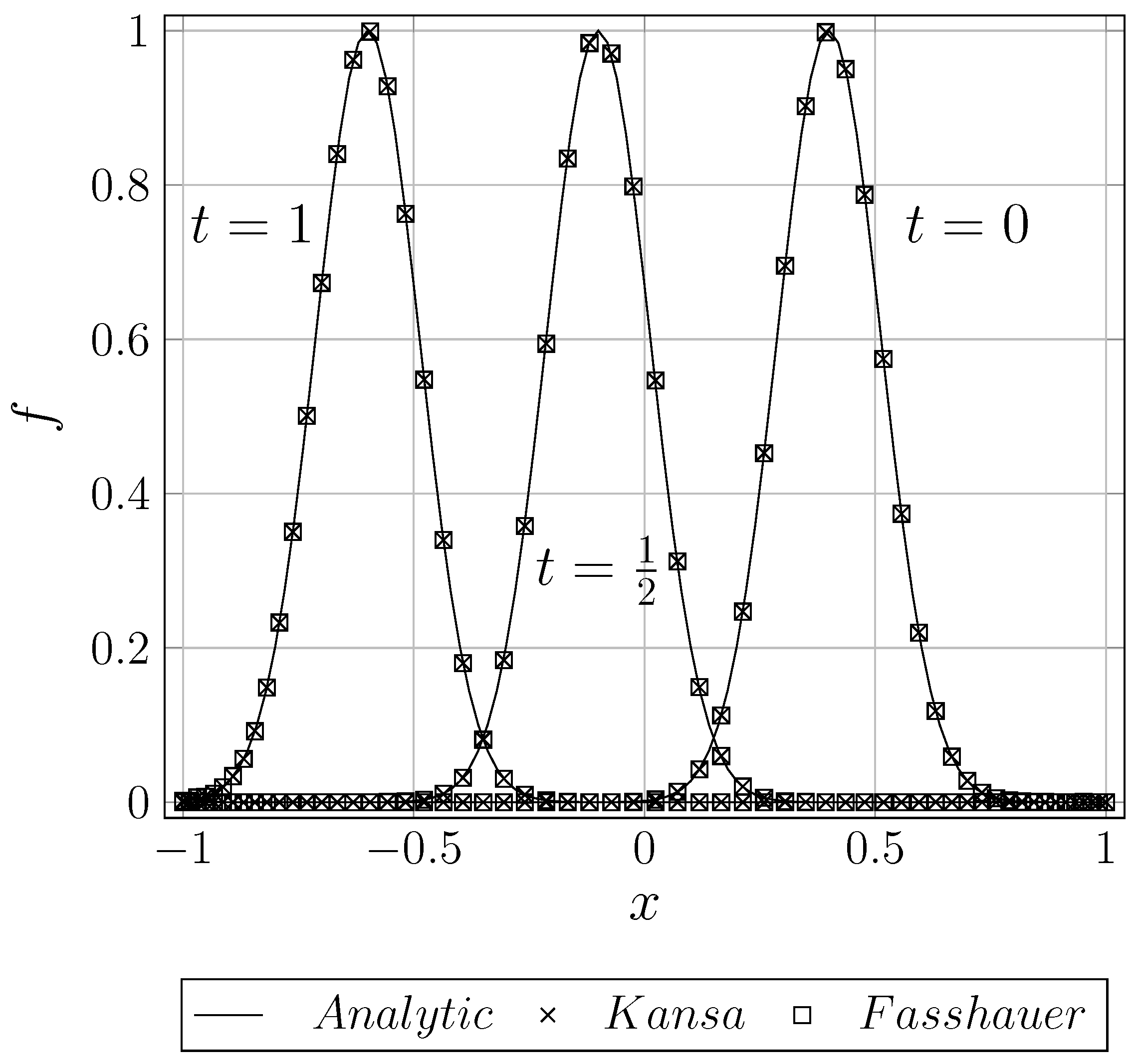
The analytical solution of the PDE is expressed as (), which was used to validate the numerical solution and to find the boundary conditions. The numerical solution procedure of Kansa’s and Fasshauer’s approaches was used to compare the predicted results at times with 60 stretched mesh points; ; ; and . The results are plotted in Figure 6. It is evident that the dissipation and dispersion errors are negligible and that the results are in good agreement with the analytical solution. It is also important to perform a quantitative comparison, this can be carried out by varying the truncation order and shape parameter and observing the effect on the error (the difference between the analytical and numerical results).
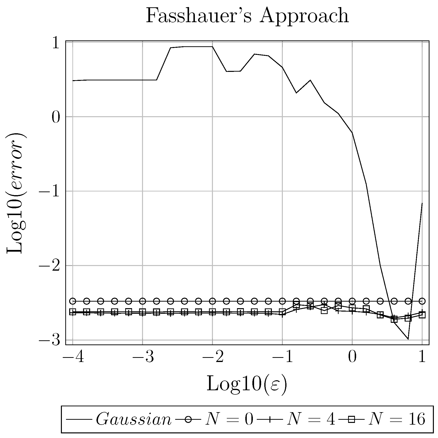
The numerical solutions achieved after 1 second by utilizing the Gaussian RBF and the new Hermite expansion approaches were compared with the analytical solution over a range of shape parameter values. The results are plotted in Figure 7. It is observed that the current approach outperforms the Gaussian RBF because it has higher accuracy over the studied range. In general, there is no significant difference between Kansa’s and Fasshauer’s approaches. However, Kansa’s approach achieves marginally higher accuracy when using the present Hermite expansion approach.
5. Conclusions
This work proposed the application of the Hermite expansion, with respect to the shape parameter, to the Gaussian RBF in order to improve the RBF method for low shape parameter () values. It was observed that the proposed expansion can be expressed either directly or recursively. The new Hermite expansion approach was compared with the Gaussian RBF approach by varying the shape parameter and then by varying the mesh size for one- and two-dimensional model functions. The obtained results illustrate that the proposed Hermite expansion approach improves accuracy and provides consistent results regardless of the shape parameter value. However, the convergence depends on the order of the truncation of the expansion. The direct and recursive approaches for evaluating the Hermite expansion were compared. The results indicate that the difference in the error between the two approaches is less than a single significant digit, which is negligible. The proposed Hermite expansion approach was used to solve the one-dimensional advection equation. The results show that the current approach outperforms the Gaussian RBF because it has higher accuracy over a wider range of . Furthermore, the proposed approach overcomes the issue of instability at small values of the shape parameter. It is concluded that the proposed Hermite expansion approach outperforms the Gaussian RBF approach, particularly for small shape parameter values.
Author Contributions
The contribution of each author is summarized as follow: conceptualization, S.A.B.; methodology, and software, S.A.B. and S.S.B.; validation, formal analysis, investigation, draft of the paper, and editing, A.M.; data curation, S.A.B., S.S.B., and A.M.; visualization, supervision, and project administration, A.M.
Funding
This research received no external funding.
Acknowledgments
This research was supported by the Ministry of Higher Education of Saudi Arabia and NSERC (National Science Engineering Research Council of Canada). We would also like to show our gratitude to the “anonymous” reviewers for their so-called insights.
Conflicts of Interest
The authors declare no conflict of interests. The funders had no role in the design of the study; in the collection, analyses, or interpretation of data; in the writing of the manuscript, or in the decision to publish the results.
References
- Kansa, E.J. Multiquadrics A scattered data approximation scheme with applications to computational fluid-dynamics—I surface approximations and partial derivative estimates. Comput. Math. Appl. 1990, 19, 127–145. [Google Scholar] [CrossRef]
- Kansa, E.J. Multiquadrics A scattered data approximation scheme with applications to computational fluid-dynamics—II solutions to parabolic, hyperbolic and elliptic partial differential equations. Comput. Math. Appl. 1990, 19, 147–161. [Google Scholar] [CrossRef]
- Fasshauer, G.E. Solving Partial Differential Equations by Collocation with Radial Basis Functions. In Proceedings of Chamonix; Vanderbilt University Press: Nashville, TN, USA, 1996; Volume 1997, pp. 1–8. [Google Scholar]
- Jumarhon, B.; Amini, S.; Chen, K. The Hermite collocation method using radial basis functions. Eng. Anal. Bound. Elem. 2000, 24, 607–611. [Google Scholar] [CrossRef]
- Zhang, X.; Song, K.; Lu, M.; Liu, X. Meshless methods based on collocation with radial basis functions. Comput. Mech. 2000, 26, 333–343. [Google Scholar] [CrossRef]
- Power, H.; Barraco, V. A comparison analysis between unsymmetric and symmetric radial basis function collocation methods for the numerical solution of partial differential equations. Comput. Math. Appl. 2002, 43, 551–583. [Google Scholar] [CrossRef] [Green Version]
- Fasshauer, G.E. RBF collocation methods as pseudospectral methods. WIT Trans. Model. Simul. 2005, 39, 47–56. [Google Scholar]
- La Rocca, A.; Rosales, A.H.; Power, H. Radial basis function Hermite collocation approach for the solution of time dependent convection–diffusion problems. Eng. Anal. Bound. Elem. 2005, 29, 359–370. [Google Scholar] [CrossRef]
- Wright, G.B.; Fornberg, B. Scattered node compact finite difference-type formulas generated from radial basis functions. J. Comput. Phys. 2006, 212, 99–123. [Google Scholar] [CrossRef]
- Sanyasiraju, Y.; Satyanarayana, C. Local Hermite-RBF based grid-free scheme with a variable (optimal) shape parameter for steady convection-diffusion equations. Int. J. Numer. Anal. Model. Ser. B 2013, 4, 382–393. [Google Scholar]
- Rocca, A.L.; Power, H. A double boundary collocation Hermitian approach for the solution of steady state convection–diffusion problems. Comput. Math. Appl. 2008, 55, 1950–1960. [Google Scholar] [CrossRef]
- Stevens, D.; Power, H.; Lees, M.; Morvan, H. The use of PDE centres in the local RBF Hermitian method for 3D convective-diffusion problems. J. Comput. Phys. 2009, 228, 4606–4624. [Google Scholar] [CrossRef]
- La Rocca, A.; Power, H.; La Rocca, V.; Morale, M. A meshless approach based upon radial basis function hermite collocation method for predicting the cooling and the freezing times of foods. CMC Tech Sci. Press 2005, 2, 239. [Google Scholar]
- Gutierrez, G.; Baquero, O.; Valencia, J.; Florez, W. Extending the local radial basis function collocation methods for solving semi-linear partial differential equations. WIT Trans. Model. Simul. 2009, 49, 117–128. [Google Scholar] [Green Version]
- Stevens, D.; LaRocca, A.; Power, H.; LaRocca, V. A Generalised RBF Finite Difference Approach to Solve Nonlinear Heat Conduction Problems on Unstructured Datasets. In Convection and Conduction Heat Transfer; InTech Open: London, UK, 2011. [Google Scholar] [Green Version]
- Bustamante Chaverra, C.A.; Power, H.; Florez Escobar, W.F.; Hill Betancourt, A.F. Two-Dimensional Meshless Solution of the Non-Linear Convection-Diffusion-Reaction Equation by the Local Hermitian Interpolation Method. Ing. Cienc. 2013, 9, 21–51. [Google Scholar] [CrossRef]
- Libre, N.; Emdadi, A.; Kansa, E.; Rahimian, M.; Shekarchi, M. Stable PDE solution methods for large multiquadric shape parameters. CMES Comput. Model. Eng. Sci. 2008, 25, 23–41. [Google Scholar]
- Beatson, R.K.; Levesley, J.; Mouat, C. Better bases for radial basis function interpolation problems. J. Comput. Appl. Math. 2011, 236, 434–446. [Google Scholar] [CrossRef] [Green Version]
- De Marchi, S.; Santin, G. A new stable basis for radial basis function interpolation. J. Comput. Appl. Math. 2013, 253, 1–13. [Google Scholar] [CrossRef]
- Rashidinia, J.; Fasshauer, G.; Khasi, M. A stable method for the evaluation of Gaussian radial basis function solutions of interpolation and collocation problems. Comput. Math. Appl. 2016, 72, 178–193. [Google Scholar] [CrossRef]
- Yurova, A.; Kormann, K. Stable evaluation of Gaussian radial basis functions using Hermite polynomials. arXiv, 2017; arXiv:1709.02164. [Google Scholar]
- Cavoretto, R.; De Rossi, A.; Perracchione, E. RBF-PU Interpolation with Variable Subdomain Sizes and Shape Parameters. In AIP Conference Proceedings; AIP Publishing: Melville, NY, USA, 2016; Volume 1776, p. 070003. [Google Scholar]
- Cavoretto, R.; De Marchi, S.; De Rossi, A.; Perracchione, E.; Santin, G. Partition of unity interpolation using stable kernel-based techniques. Appl. Numer. Math. 2017, 116, 95–107. [Google Scholar] [CrossRef] [Green Version]
- Fornberg, B.; Piret, C. A stable algorithm for flat radial basis functions on a sphere. SIAM J. Sci. Comput. 2007, 30, 60–80. [Google Scholar] [CrossRef]
- Fornberg, B.; Larsson, E.; Flyer, N. Stable Computations with Gaussian Radial Basis Functions in 2-D; Technical Report 2009-020; Uppsala University, Division of Scientific Computing: Uppsala, Sweden, 2009. [Google Scholar]
- Fornberg, B.; Larsson, E.; Flyer, N. Stable computations with Gaussian radial basis functions. SIAM J. Sci. Comput. 2011, 33, 869–892. [Google Scholar] [CrossRef]
- Larsson, E.; Lehto, E.; Heryudono, A.; Fornberg, B. Stable computation of differentiation matrices and scattered node stencils based on gaussian radial basis functions. SIAM J. Sci. Comput. 2013, 35, A2096–A2119. [Google Scholar] [CrossRef]
- Fornberg, B.; Lehto, E.; Powell, C. Stable calculation of Gaussian-based RBF-FD stencils. Comput. Math. Appl. 2013, 65, 627–637. [Google Scholar] [CrossRef]
- Gonnet, P.; Pachón, R.; Trefethen, L.N. Robust rational interpolation and least-squares. Electron. Trans. Numer. Anal. 2011, 38, 146–167. [Google Scholar]
- Wright, G.B.; Fornberg, B. Stable computations with flat radial basis functions using vector-valued rational approximations. J. Comput. Phys. 2017, 331, 137–156. [Google Scholar] [CrossRef] [Green Version]
- Fasshauer, G.E. Meshfree Approximation Methods with MATLAB; World Scientific: Singapore, 2007. [Google Scholar] [CrossRef]
- Lebedev, N.N. The Special Functions and Their Applications; Dover Publications: New York, NY, USA, 1965. [Google Scholar]
- Sarra, S.A.; Kansa, E.J. Multiquadric Radial Basis Function Approximation Methods for the Numerical Solution of Partial Differential Equations. In Advances in Computational Mechanics; Tech Science Press: Henderson, NV, USA, 2009; Volume 2. [Google Scholar]
Figure 1.
Comparison between the Gaussian radial basis function (RBF) and proposed Hermite expansion of the RBF for approximating the one-dimensional model equation and its derivatives.
Figure 1.
Comparison between the Gaussian radial basis function (RBF) and proposed Hermite expansion of the RBF for approximating the one-dimensional model equation and its derivatives.

Figure 2.
Error in approximating the given function and its first two derivatives using Gaussian RBF approach and Hermite expansion approaches as they vary with . The number of mesh points is fixed at 80 stretched points within the range [−1,1].
Figure 2.
Error in approximating the given function and its first two derivatives using Gaussian RBF approach and Hermite expansion approaches as they vary with . The number of mesh points is fixed at 80 stretched points within the range [−1,1].

Figure 3.
Error of approximating the specified function and its derivatives using the Gaussian RBF approach and Hermite expansion approach as they vary with . The number of mesh points is fixed at 900, they are randomly distributed within the range [−1,1].
Figure 3.
Error of approximating the specified function and its derivatives using the Gaussian RBF approach and Hermite expansion approach as they vary with . The number of mesh points is fixed at 900, they are randomly distributed within the range [−1,1].

Figure 4.
Error of approximating the specified function and its derivatives using the Gaussian RBF approach and Hermite expansion approach as they vary with the mesh size (). The shape parameter is fixed at . The mesh points are stretched points within the range [−1,1].
Figure 4.
Error of approximating the specified function and its derivatives using the Gaussian RBF approach and Hermite expansion approach as they vary with the mesh size (). The shape parameter is fixed at . The mesh points are stretched points within the range [−1,1].

Figure 5.
Comparison between direct and recursive approaches by varying for a specified function and its first two derivatives. The number of mesh points is fixed at 80 stretched points within the range [−1,1].
Figure 5.
Comparison between direct and recursive approaches by varying for a specified function and its first two derivatives. The number of mesh points is fixed at 80 stretched points within the range [−1,1].

Figure 6.
Comparison between Kansa’s and Fasshauer’s approaches at for the advection partial differential equation at times ; ; and . The number of mesh points is fixed at 60 stretched points within the range [−1,1].
Figure 6.
Comparison between Kansa’s and Fasshauer’s approaches at for the advection partial differential equation at times ; ; and . The number of mesh points is fixed at 60 stretched points within the range [−1,1].

Figure 7.
Comparison between Kansa’s and Fasshauer’s approaches for solving the advection partial differential equation at different values. The number of mesh points is fixed at 60 stretched points within the range [−1,1].
Figure 7.
Comparison between Kansa’s and Fasshauer’s approaches for solving the advection partial differential equation at different values. The number of mesh points is fixed at 60 stretched points within the range [−1,1].


Table 1.
Values of first few terms of and its derivatives.
| n | |||||
|---|---|---|---|---|---|
| 0 | |||||
| 2 | |||||
| 4 | |||||
| 6 |
© 2019 by the authors. Licensee MDPI, Basel, Switzerland. This article is an open access article distributed under the terms and conditions of the Creative Commons Attribution (CC BY) license (http://creativecommons.org/licenses/by/4.0/).
Share and Cite
MDPI and ACS Style
Bawazeer, S.A.; Baakeem, S.S.; Mohamad, A. A New Radial Basis Function Approach Based on Hermite Expansion with Respect to the Shape Parameter. Mathematics 2019, 7, 979. https://0-doi-org.brum.beds.ac.uk/10.3390/math7100979
AMA Style
Bawazeer SA, Baakeem SS, Mohamad A. A New Radial Basis Function Approach Based on Hermite Expansion with Respect to the Shape Parameter. Mathematics. 2019; 7(10):979. https://0-doi-org.brum.beds.ac.uk/10.3390/math7100979
Chicago/Turabian StyleBawazeer, Saleh Abobakur, Saleh Saeed Baakeem, and Abdulmajeed Mohamad. 2019. "A New Radial Basis Function Approach Based on Hermite Expansion with Respect to the Shape Parameter" Mathematics 7, no. 10: 979. https://0-doi-org.brum.beds.ac.uk/10.3390/math7100979
Note that from the first issue of 2016, this journal uses article numbers instead of page numbers. See further details here.