Dynamic Restructuring Framework for Scheduling with Release Times and Due-Dates


Centro de Investigación en Ciencias, Universidad Autónoma del Estado de Morelos, Morelos 62209, Mexico
Mathematics 2019, 7(11), 1104; https://0-doi-org.brum.beds.ac.uk/10.3390/math7111104
Submission received: 8 October 2019
/
Revised: 5 November 2019
/
Accepted: 12 November 2019
/
Published: 14 November 2019
(This article belongs to the Special Issue Advances and Novel Approaches in Discrete Optimization)
Abstract
:Scheduling jobs with release and due dates on a single machine is a classical strongly NP-hard combination optimization problem. It has not only immediate real-life applications but also it is effectively used for the solution of more complex multiprocessor and shop scheduling problems. Here, we propose a general method that can be applied to the scheduling problems with job release times and due-dates. Based on this method, we carry out a detailed study of the single-machine scheduling problem, disclosing its useful structural properties. These properties give us more insight into the complex nature of the problem and its bottleneck feature that makes it intractable. This method also helps us to expose explicit conditions when the problem can be solved in polynomial time. In particular, we establish the complexity status of the special case of the problem in which job processing times are mutually divisible by constructing a polynomial-time algorithm that solves this setting. Apparently, this setting is a maximal polynomially solvable special case of the single-machine scheduling problem with non-arbitrary job processing times.
1. Introduction
Scheduling jobs with release and due-dates on single machine is a classical strongly NP-hard combination optimization problem according to Garey and Johnson [1]. In many practical scheduling problems, jobs are released non-simultaneously and they have individual due-dates by which they ideally have to complete. Since the problem is NP-hard, the existing exact solution algorithms have an exponential worst-case behavior. The problem is important not only because of its immediate real-life applications, but also because it is effectively used as an auxiliary component for the solution of more complex multiprocessor and shop scheduling problems.
Here, we propose a method that can, in general, be applied to the scheduling problems with job release times and due-dates. Based on this method, we carry out a detailed study of the single-machine scheduling problem disclosing its useful structural properties. These properties give us more insight into the complex nature of the problem and its bottleneck feature that makes it intractable. At the same time, the method also helps us to expose explicit conditions when the problem can be solved in polynomial time. Using the method, we establish the complexity status of the special case of the problem in which job processing times are mutually divisible by constructing a polynomial-time algorithm that solves this setting. This setting is a most general polynomially solvable special case of the single-machine scheduling problem when jobs have restricted processing times but job parameters are not bounded: if job processing times are allowed to take arbitrary values from set , for an integer p, the problem remains strongly NP-hard [2]. At the same time, the restricted setting may potentially have practical applications in operating systems (we address this issue in more detail in Section 12).
Problem description. Our problem, commonly abbreviated in the scheduling literature as (the notation suggested by Graham et al. [3]), can be stated as follows. There are given n jobs and a single machine. Each job j has (uninterruptible) processing time , release time and due-date: is the time required by job j on the machine; is the time moment by which job j becomes available for scheduling on the machine; and is the time moment, by which it is desirable to complete job j on the machine (informally, the smaller is job due-date, the more urgent it is, and the late completion is penalized by the objective function).
The problem restrictions are as follows. The first basic restriction is that the machine can handle at most one job at a time.
A feasible schedule S is a mapping that assigns to every job j its starting time on the machine, such that
and
for any job k included earlier in S (for notational simplicity, we use S also for the corresponding job-set).
The inequality in Equation (1) ensures that no job is started before its release time, and the inequality in Equation (2) ensures that no two jobs overlap in time on the machine.
is the completion time of job j in schedule S.
The delay of job j in schedule S is
An optimal schedule is a feasible schedule minimizing the maximum job lateness
(besides the lateness, there exist other due-date oriented objective functions). (, respectively) stands for the maximum job lateness in schedule S (the lateness of job j in S, respectively). The objective is to find an optimal schedule.
Adopting to the standard three-field scheduling notation, we abbreviate the special case of problem with divisible job processing times by . In that setting, we restrict job processing times to the mutually divisible ones: given any two neighboring elements in a sequence of job processing times ordered non-decreasingly, the first one exactly divides the second one (this ratio may be 1). A typical such sequence is formed by the integers each of which is (an integer) power of 2 multiplied by an integer .
A brief introduction to our method. Job release times and due-dates with due-date orientated objective functions compose a sloppy combination for most of the scheduling problems in the sense that it basically contributes to their intractability. In such problems, the whole scheduling horizon can be partitioned, roughly, into two types of intervals, the rigid one and the flexible ones. In an optimal schedule, every rigid interval (that potentially may contribute to the optimal objective value) is occupied by a specific set of (urgent) jobs, whereas the flexible intervals can be filled out by the rest of the (non-urgent) jobs in different ways. Intuitively, the “urgency” of a job is determined by its due-date and the due-dates of close-by released jobs; a group of such jobs may form a rigid sequence in a feasible schedule if the differences between their due-dates are “small enough”. The remaining jobs are to be “dispelled” in between the rigid sequences.
This kind of division of the scheduling horizon, which naturally arises in different machine environments, reveals an inherent relationship of the scheduling problems with a version of bin packing problem and gives some insight into a complicated nature of the scheduling problems with job release times and due-dates. As shown below, this relationship naturally yields a general algorithmic framework based on the binary search.
A bridge between the scheduling and the bin packing problems is constructed by a procedure that partitions the scheduling horizon into the rigid and the flexible intervals. Exploring a recurrent nature of the scheduling problem, we develop a polynomial-time recursive procedure that partitions the scheduling horizon into the rigid and flexible intervals. After this partition, the scheduling of the rigid intervals is easy but scheduling of the flexible intervals remains non-trivial. Optimal scheduling of the flexible intervals, despite the fact that these intervals are formed by non-urgent jobs, remains NP-hard. To this end, we establish further structural properties of the problem, which yield a general algorithmic framework that may require exponential time. Nevertheless, we derive a condition when the framework will find an optimal solution in polynomial time. This condition reveals a basic difficulty that would face any polynomial-time algorithm to create an optimal solution.
Some kind of compactness property for the flexible segments may be guaranteed if they are scheduled in some special way. In particular, we show that the compactness property can be achieved by an underlying algorithm that works for the mutually divisible job processing times. The algorithm employs some nice properties of a set of mutually divisible numbers.
In terms of time complexity, our algorithmic framework solves problem in time if our optimality condition is satisfied. Whenever during the execution of the framework the condition is not satisfied, an additional implicit enumeration procedure can be incorporated (to maintain this work within a reasonable size, here we focus solely to exact polynomial-time algorithms). Our algorithm for problem yields an additional factor of , so its time complexity is .
Some previous related work. Coffman, Garey and Johnson [4] previously showed that some special cases of a number of weakly NP-hard bin packing problems with divisible item sizes can be solved in polynomial time (note that our algorithm implies a similar result for a strongly NP-hard scheduling problem). We mention briefly some earlier results concerning our scheduling problem. As to the exponential-time algorithms, the performance of venerable implicit enumeration algorithms by McMahon and Florian [5] and Carlier [6] has not yet been surpassed. There is an easily seen polynomial special case of the problem when all job release times or due-dates are equal (Jackson [7]), or all jobs have unit processing times (Horn [8]). If all jobs have equal integer length p, the problem can also be solved in polynomial time . Garey et al. [9] described how the union and find tree with path compression can be used to reduce the time complexity to . The problem , in which job processing times are restricted to p and , for an integer p, can also be solved in polynomial time [10]. If we bound the maximum job processing time by a polynomial function in n, , and the maximal difference between the job release times by a constant R, then the problem remains polynomially solvable [2]. When is a constant or it is , the time complexity of the algorithm by [2] is ; for , it is . The algorithm becomes pseudo-polynomial without the restriction on and it becomes exponential without the restriction on job release times. In another polynomially solvable special case the jobs can be ordered so that and , for some and Lazarev and Arkhipov [11]. The problem allows fast solution if for any pair of jobs with and , , and if then [12].
The structure of this work. This paper consists of two major parts. In Part 1, an algorithmic framework for a single machine environment and a common due-date oriented objective function, the maximum job lateness, is presented, whereas, in Part 2, the framework is finished to a polynomial-time algorithm for the special case of the problem with mutually divisible job processing times. In Section 2, we give a brief informal introduction to our method. Section 3 contains a brief overview of the basic concepts and some basic structural properties that posses the schedules enumerated in the framework. In Section 4, we study recurrent structural properties of our schedules, which permit the partitioning of the scheduling horizon into the two types of intervals. In Section 5, we describe how our general framework is incorporated into a binary search procedure. In Section 6, we give an aggregated description of our main framework based on the partitioning of the scheduling horizon into the flexible and the rigid segments, and show how the rigid segments are scheduled in an optimal solution. In Section 7, we describe a procedure which is in charge of the scheduling of the non-urgent segments, and formulate our condition when the main procedure will deliver an optimal solution. This completes Part 1. Part 2 consists of Section 8, Section 9, Section 10 and Section 11, and is devoted to the version of the general single-machine scheduling problem with mutually divisible job processing times (under the assumption that the optimality condition of Section 7 is not satisfied). In Section 8, we study the properties of a set of mutually divisible numbers that we use to reduce the search space. Using these properties, we refine our search in Section 9. In Section 10, we give the final examples illustrating the algorithm for divisible job processing times. In Section 11, we complete the correctness proof of that algorithm. The conclusions in Section 12 contain final analysis, possible impact, extensions and practical applications of the proposed method and the algorithm for the divisible job processing times.
2. An Informal Description of the General Framework
In this section, we give a brief informal introduction to our method (the reader may choose to skip it and go to formal definitions of the next section). We mention above the ties of our scheduling problem with a version of bin packing problem, in which there is a fixed number of bins of different capacities and the objective is to find out if there is a feasible solution respecting all the bin capacities. To see the relationship between the bin packing and the scheduling problems, we analyze the structure of the schedules that we enumerate. In particular, the scheduling horizon will contain two types of sequences formed by the “urgent” jobs (that we call kernels) and the remaining sequences formed by the “non-urgent” jobs (that we call bins). A key observation is that a kernel may occupy a quite restricted time interval in any optimal schedule, whereas the bin intervals can be filled out by the non-urgent jobs in different ways. In other words, the urgent jobs are to be scheduled within the rigid time intervals, whereas non-urgent ones are to be dispelled within the flexible intervals. Furthermore, the time interval within which each kernel is to be scheduled can be “adjusted” in terms of the delay of its earliest scheduled job. In particular, it suffices to consider the feasible schedules in which the earliest job of a kernel K is delayed by at most some magnitude, e.g., ; , where is the initial delay of the earliest scheduled job of that kernel (intuitively, can be seen as an upper bound on the possible delay for kernel K, a magnitude, by which the earliest scheduled job of kernel K can be delayed without surpassing the minimal so far achieved maximum job lateness). As shown below, for any kernel K, . Observe that, if , i.e., when we restrict our attention to the feasible schedules in which kernel K has no delay, the lateness of the latest scheduled job of that kernel is a lower bound on the optimal objective value. In this way, we can calculate the time intervals which are to be assigned to every kernel relatively easily. The bins are formed by the remaining time intervals. The length of a bin, i.e., that of the corresponding time interval, will not be prior fixed until the scheduling of that bin is complete (roughly, because there might be some valid range for the “correct” s).
Then, roughly, the scheduling problem reduces to finding out if all the non-kernel jobs can “fit” feasibly (with respect to their release times) into the bins without surpassing the currently allowable lateness for the kernel following that bin; recall that the “allowable lateness” of kernel K is determined by . We “unify” all the s to a single (common for all the kernels), and carry out binary search to find an optimal within the interval (the minimum such that all the non-kernel jobs fit into the bins; the less is , the less is the imposed lateness for the kernel jobs).
Thus, there is a fixed number of bins of different capacities (which are the lengths of the corresponding intervals in our setting), and the items which are to be assigned to these bins are non-kernel jobs. We aim to find out if these items can feasibly be packed into these bins. A simplified version of this problem, in which no specified time interval with each bin is associated and the items can be packed in any bin, is NP-hard. In our version, whether a job can be assigned to a bin depends, in a straightforward way, on the interval of that bin and on the release time of that job (a feasible packing is determined according to these two parameters).
If the reader is not yet too confused, we finally note that the partition of jobs into kernel and non-kernel ones is somewhat non-permanent: during the execution of our framework, a non-kernel job may be “converted” into a kernel one. This kind of situation essentially complicates the solution process and needs an extra treatment. Informally, this causes the strong NP-hardness of the scheduling problem: our framework will find an optimal solution if no non-kernel job converts to a kernel one during its execution (the so-called instance of Alternative (b2)). We observe this important issue in later sections, starting from Section 7.
3. Basic Definitions
This subsection contains definitions which consequently gain in structural insight of problem (see, for instance, [2,13]). First, we describe our main schedule generation tool. Jackson’s extended heuristics (Jackson [7] and Schrage [14]), also referred to as the Earliest Due-date heuristics (ED-heuristics), is commonly used for scheduling problems with job release times and due-dates. ED-heuristics is characterized by n scheduling times: these are the time moments at which a job is assigned to the machine. Initially, the earliest scheduling time is set to the minimum job release time. Among all jobs released by a given scheduling time (the jobs available by that time moment), one with the minimum due-date is assigned to the machine (ties can be broken by selecting a longest job). Iteratively, the next scheduling time is the maximum between the completion time of the latest assigned so far job to the machine and the minimum release time of a yet unassigned job (note that no job can be started before the machine gets idle, and no job can be started before its release time). Among all jobs available by each scheduling time, a job with the minimum due-date is determined and is scheduled on the machine at that time. Thus, whenever the machine becomes idle, ED-heuristics schedules an available job giving the priority to a most urgent one. In this way, it creates no gap that can be avoided (by scheduling some already released job).
3.1. Structural Components in an ED-Schedule
While constructing an ED-schedule, a gap (an idle machine-time) may be created (a maximal consecutive time interval during which the machine is idle; by our convention, there occurs a 0-length gap if job i is started at its release time immediately after the completion of job j.
An ED-schedule can be seen as a sequence of somewhat independent parts, the so-called blocks; each block is a consecutive part in that schedule that consists of a sequence of jobs successively scheduled on the machine without any gap in between any neighboring pair of them; a block is preceded and succeeded by a (possibly a 0-length) gap.
As shown below in this subsection, by modifying the release times of some jobs, ED-heuristics can be used to create different feasible solutions to problem . All feasible schedules that we consider are created by ED-heuristics, which we call ED-schedules. We construct our initial ED-schedule, denoted by , by applying ED-heuristics to the originally given problem instance. Then, we slightly modify the original problem instance to generate other feasible ED-schedules.
Kernels. Now, we define our kernels and the corresponding bins formally. Recall that kernel jobs may only occupy restricted intervals in an optimal schedule, whereas the remaining bin intervals are to be filled in by the rest of the jobs (the latter jobs are more flexible because they may be “moved freely” within the schedule, without affecting the objective value to a certain degree, as we show below).
Let be a block in an ED-schedule S containing job o that realizes the maximum job lateness in that schedule, i.e.,
Among all jobs in block satisfying Equation (3), the latest scheduled one is called an overflow job in schedule S.
A kernel in schedule S is a longest continuous job sequence ending with an overflow job o, such that no job from this sequence has a due-date greater than (for notational simplicity, we use K also for the corresponding job-set). For a kernel K, we let . We may observe that the number of kernels in schedule S equals to the number of the overflow jobs in it. Besides, since every kernel is contained within a single block, it may include no gap. We denote by the earliest kernel in schedule S. The following proposition states an earlier known fact from [13]. Nevertheless, we also give its proof as it gains some intuition on the used here techniques.
Proposition 1.
The maximum lateness of a job of kernel K in ED-schedule S is the minimum possible if the earliest scheduled job of that kernel starts at time . Hence, if schedule S contains a kernel with this property, then it is optimal.
Proof.
By the definition, for any job , (job j is no-less urgent than the overflow job o), whereas note that the maximum lateness of a job of kernel K in schedule S is . At the same time, the jobs in kernel K form a tight (continuous) sequence without any gap. Let be a complete schedule in which the order of jobs of kernel K differs to that in schedule S and let job realizes the maximum lateness of a job of kernel K in schedule . Then, from the above observations and the fact that the earliest job of kernel K starts at its release time in schedule S, it follows that
Hence,
and schedule S is optimal. □
Emerging jobs. In the rest of this section, let S be an ED-schedule with kernel and with the overflow job such that the condition in Proposition 1 does not hold. That is, there exists job e with scheduled before all jobs of kernel K that imposes a forced delay (right-shift) for the jobs of that kernel. By creating an alternative feasible schedule in which job e is rescheduled after kernel K, this kernel may be (re)started earlier, i.e., the earliest scheduled job of kernel K may be restarted earlier than the earliest scheduled job of that kernel has started in schedule S. We need some extra definitions before we define the so-obtained alternative schedule formally.
Suppose job i precedes job j in ED-schedule S. We say that i pushes j in S if ED-heuristics may reschedule job j earlier if job i is forced to be scheduled after job j.
If (by the made assumption immediately behind Proposition 1) the earliest scheduled job of kernel K does not start at its release time, then it is immediately preceded and pushed by Job l with , the so-called delaying emerging job for kernel K (we use l exclusively for the delaying emerging job).
Besides the delaying emerging job, there may exist job e with scheduled before kernel K (hence before Job l) in schedule S pushing jobs of kernel K in schedule S. Any such job as well as Job l is referred to as an emerging job for K.
We denote the set of emerging jobs for kernel K in schedule S by . Note that and since S is an ED-schedule, , for any , as otherwise a job of kernel K with release time would have been included at the starting time of job e in schedule S.
Besides jobs of set , schedule S may contain job j satisfying the same parametric conditions as an emerging job from set , i.e., and , but scheduled after kernel K. We call such a job a passive emerging job for kernel K (or for the overflow job o) in schedule S. We denote the set of all the passive emerging jobs for kernel by .
Note that any is included in block (the block in schedule S containing kernel K) in schedule S. Note also that, potentially, any job can be feasibly scheduled before kernel K as well. A job not from set is a non-emerging job in schedule S.
In summary, all jobs in are less urgent than all jobs of kernel K and any of them may be included before or after that kernel within block . The following proposition is not difficult to prove (e.g., see [13]).
Proposition 2.
Let be a feasible schedule obtained from schedule S by the rescheduling a non-emerging job of schedule S after kernel K. Then, The inequality in Equation (4) holds.
Activation of an emerging job. Because of the above proposition, it suffices to consider only the rearrangements in schedule S that involve the jobs from set . As the first pass, to restart kernel K earlier, we may create a new ED-schedule obtained from schedule S by the rescheduling an emerging job after kernel K (we call this operation the activation of job e for kernel K). In ED-schedule , besides job e, all jobs in are also scheduled (remain to be scheduled) after kernel K. Technically, we create schedule by increasing the release times of job e and jobs in to a sufficiently large magnitude (e.g., the maximum job release time in kernel K), so that, when ED-heuristics is newly applied, neither job e nor any of the jobs in set will be scheduled before any job of kernel K.
It is easily seen that kernel K (regarded as a job-set) restarts earlier in ED-schedule than it has started in schedule S. In particular, the earliest job of kernel K is immediately preceded by a gap and starts at time in schedule , whereas the earliest scheduled job of kernel K in schedule S starts after time (the reader may have a look at the work of Vakhania, N. [13] for more details on the relevant issues).
L-schedules. We call a complete feasible schedule in which the lateness of no job is more than threshold L, an L-schedule. In schedule S, job i is said to surpass the L-boundary if .
The magnitude
is called the L-delay of job i in schedule S.
3.2. Examples
We illustrate the above introduced notions in the following two examples.
Example 1.
We have a problem instance with four jobs , defined as follows:
,
,
.
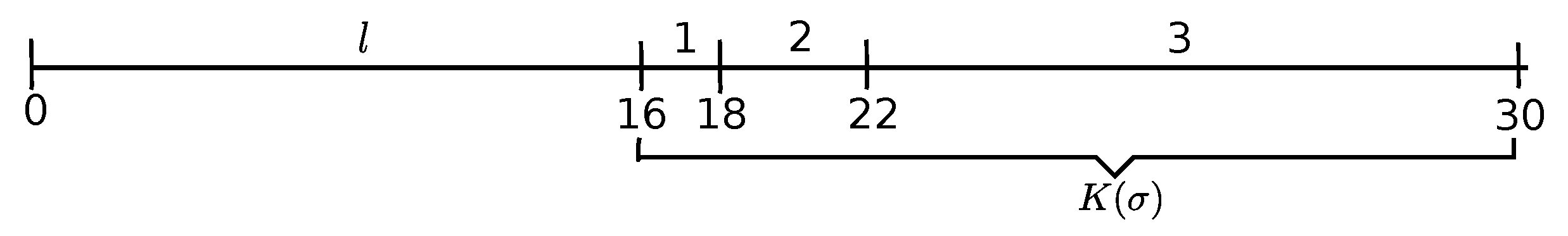
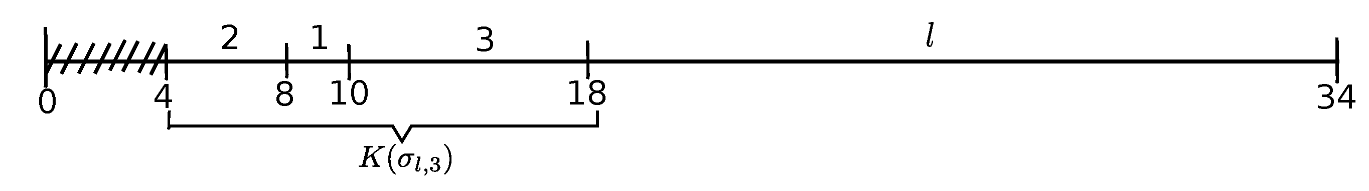
The initial ED-schedule is illustrated in Figure 1. There is a single emerging job in that schedule, which is the delaying emerging Job l pushing the following scheduled Jobs 1–3, which constitute the kernel in ; Job 3 is the overflow job o in schedule , which consists of a single block. .
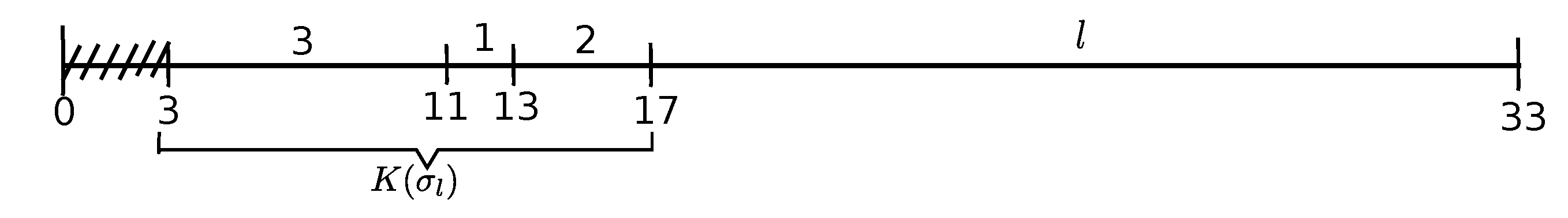
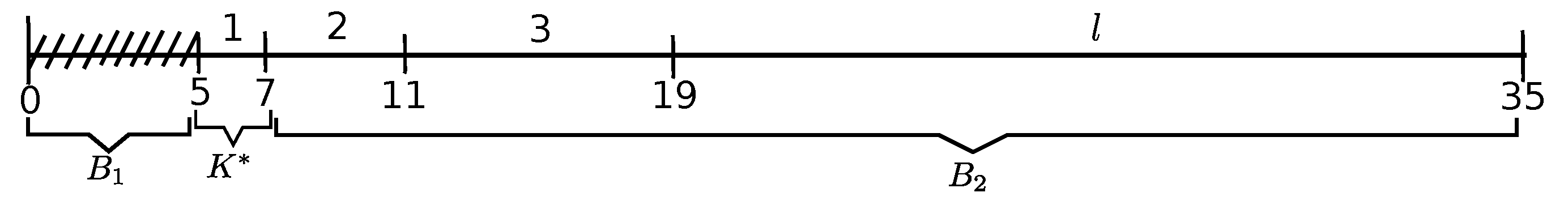
ED-schedule , depicted in Figure 2, is obtained by activating the delaying emerging Job l in schedule (the release time of Job l is set to that of job 1 and ED-heuristics is newly applied). Kernel in that schedule is formed by Jobs 1 and 2, Job 2 is the overflow job with , whereas Job 3 becomes the delaying emerging job in schedule .
Example 2.
In our second (larger) problem instance, we have eight jobs , defined as follows:
,
,
,
,
,
,
.
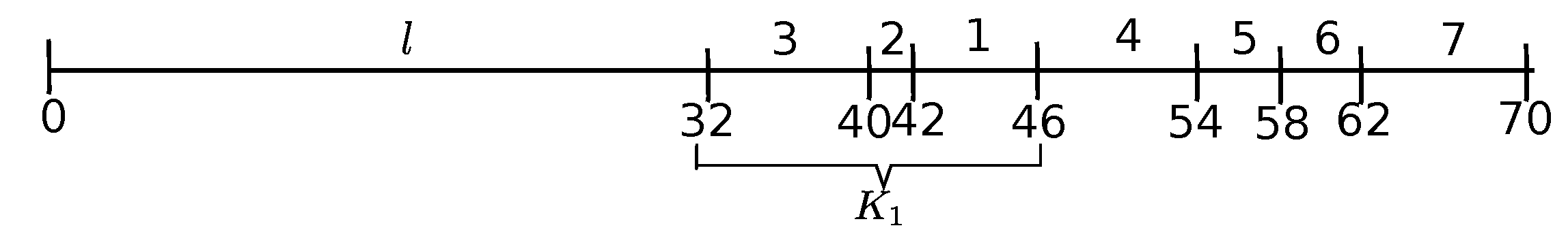
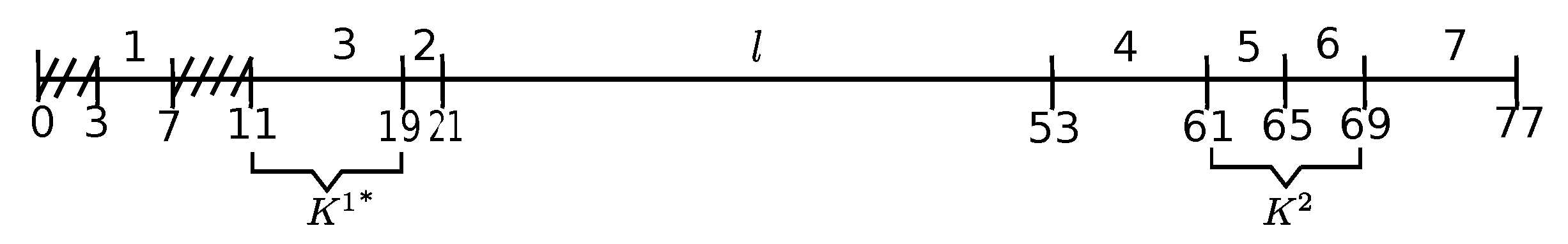
The initial ED-schedule is illustrated in Figure 3. Job l is the delaying emerging job, and Jobs 4 and 7 are passive emerging jobs. The kernel is formed by Jobs 3, 2, and 1 (Job 1 being the overflow job).
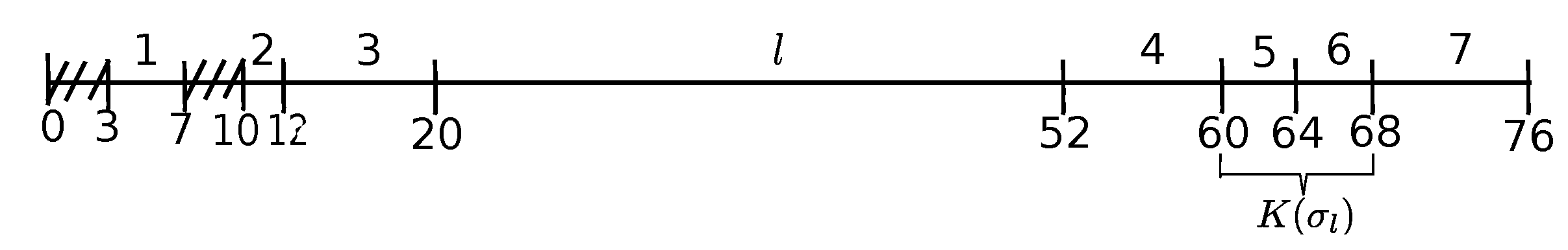
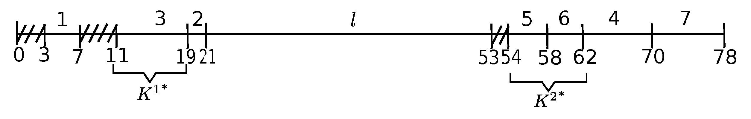
ED-schedule is depicted in Figure 4. There arises a (new) kernel formed by Jobs 5 and 6, whereas Job 4 is the delaying emerging job (Job 7 is the passive emerging job for both, kernels and ). Job 6 is the overflow job, with .
4. Recurrent Substructures for Kernel Jobs
In this section, we describe a recursive procedure that permits us to determine the rigid intervals of a potentially optimal schedule (as we show below, these intervals not necessarily coincide with kernel intervals detected in ED-schedules). The procedure relies on an important recurrent substructure property, which is also helpful for the establishment of the ties of the scheduling problem with bin packing problems.
We explore the recurrent structure of our scheduling problem by analyzing ED-schedules. To start with, we observe that in ED-schedule (where l is the delaying emerging job for kernel ), the processing order of the jobs in kernel K can be altered compared to that in schedule S. Since the time interval that was occupied by Job l in schedule S gets released in schedule , some jobs of kernel K may be scheduled within that interval (recall that by the construction, no job from may occupy that interval). In fact, the processing order of jobs of kernel K in schedules S and might be different: recall from Section 3 that a job with will be included the first within the above interval in schedule (whereas kernel K in schedule S is not necessarily initiated by job j; the reader may compare ED-schedules of Figure 1 and Figure 2 and those of Figure 3 and Figure 4 of Examples 1 and 2, respectively).
We call job anticipated in schedule if it is rescheduled to an earlier position in that schedule compared to its position in schedule S (in ED-schedules of Figure 2 and Figure 4, Job 3 and Jobs 1 and 2, respectively, are the anticipated ones). In other words, job j surpasses at least one job i in schedule such that i has surpassed j in schedule S (we may easily observe that, due to ED-heuristics, this may only happen if , as otherwise job j would have been included before job i already in schedule S). Recall from Section 3 that the earliest scheduled job of kernel K is immediately preceded by a newly arisen gap in schedule (in ED-schedules of Figure 2 and Figure 4 it is the gap ). Besides, a new gap in between the jobs of kernel K may also arise in schedule if there exists an anticipated job since, while rescheduling the jobs of kernel K, there may occur a time moment at which some job of that kernel completes but no other job is available in schedule . Such a time moment in ED-schedule of Figure 4 is 7, which is extending up to the release Time 10 of Job 2 resulting in a new gap arising within the jobs of kernel .
It is apparent now that jobs of kernel K (kernel in the above example) may be redistributed into several continuous parts separated by the gaps in schedule (the first such part in ED-schedule of Figure 4. consists of the anticipated Job 1 and the second part consists of Jobs 2 and 3, where Job 2 is another anticipated job).
If there arises an anticipated job so that the jobs of kernel K are redistributed into one or more continuous parts in schedule , then kernel K is said to collapse; if kernel K collapses into a single continuous part, then this continuous part and kernel K, considered as job-sets, are the same, but the corresponding job sequences are different because of an anticipated job. It follows that, if kernel K collapses, then there is at least one anticipated job in schedule that converts to the delaying emerging job in that schedule (recall from Proposition 1 that schedule S is optimal if it possesses no delaying emerging job).
Throughout this section, we concentrate our attention to the part of schedule initiating at the starting time of Job l in schedule S and containing all the newly arisen continuous parts of kernel K in that schedule that we denote by . We treat this part as an independent ED-schedule consisting of solely the jobs of the collapsed kernel K (recall that no job distinct from a job of kernel K may be included in schedule until all jobs of kernel K are scheduled, by the definition of that schedule). For the instance of Example 1 with , schedule is the part of the ED-schedule of Figure 2 that initiates at at Time 0 and ends at Time 17. For the instance of Example 2, schedule starts at Time 0 and ends at Time 20 (see Figure 4).
We distinguish three different types of continuous parts in schedule . A continuous part that consists of only anticipated jobs (contains no anticipated job, respectively) is called an anticipated (uniform, respectively) continuous part. A continuous part which is neither anticipated nor uniform is called mixed (hence, mixed continuous part contains at least one anticipated and one non-anticipated job).
We observe that in ED-schedule of Figure 2 schedule consists of a single mixed continuous part with the anticipated Job 3, which becomes the new delaying emerging job in that schedule. Schedule of Example 2 (Figure 4) consists of two continuous parts, the first of which is anticipated with a single anticipated Job 1, and the second one is mixed with the anticipated Job 2. The latter job becomes the delaying emerging job in schedule and is followed by Job 3, which constitutes the unique kernel in schedule .
Substructure Components
The decomposition of kernel K into the continues parts has the recurrent nature. Indeed, we easily observe that schedule has its own kernel . If kernels K and (considered as sequences) are different, then the decomposition process naturally continues with kernel (otherwise, it ends by Point (4) of Proposition 3). For instance, in Example 1, kernel is constituted by Jobs 1 and 2 (Figure 2) and, in Example 2, it is constituted by Job 3 (see Figure 4) (in Lemma 4, we show that schedule may contain only one kernel, which is from the last continuous part of that schedule). In turn, if kernel possesses the delaying emerging job, it may also collapse, and this process may recurrently be repeated. This gives the rise to a recurrent substructure decomposition of kernel K. The process continues as long as the next arisen kernel may again collapse, i.e., it possesses the delaying emerging job. Suppose there is the delaying emerging job for kernel in schedule . We recurrently define a (sub)schedule of schedule containing only jobs of kernel and in which the delaying emerging job is activated for that kernel, similarly to what is done for schedule . This substructure definition applies recursively as long as every newly derived (sub)schedule contains a kernel that may collapse, i.e., it possesses the delaying emerging job (this kernel belongs to the last continuous part of the (sub)schedule, as we prove in Lemma 4). This delaying emerging job is activated and the next (sub)schedule is similarly created.
We refer to the created is this (sub)schedules as the substructure components arisen as a result of the collapsing of kernel K and the following arisen kernels during the decomposition process. As already specified, the first component in the decomposition is with kernel , the second one is with kernel , the third one is , with kernel , where is the delaying emerging job of kernel , and so on, with the last atomic component being such that the kernel of that component has no delaying emerging job (here, is the delaying emerging job of kernel ). Note that the successively created components during the decomposition form an embedded substructure in the sense that the set of jobs that contains each next generated component is a proper subset of that of the previously created one: substructure component , for any , contains only jobs of kernel , whereas clearly (as kernel does not contain, at least, job , i.e., no activated delaying emerging job pertains to the next generated substructure component).
Below, we give a formal description of the procedure that generates the complete decomposition of kernel K, i.e., it creates all the substructure components of that kernel.
PROCEDURE Decomposition
{S is an ED-schedule with kernel K and delaying emerging Job l}
WHILE is not atomic DO
BEGIN
- ; the kernel in component ;
- the delaying emerging job of component ;
- CALL PROCEDURE Decomposition
END.
We illustrate the decomposition procedure on our two problem instances.
Example 1 (continuation). In the decomposition of kernel of Example 1, in ED-schedule of Figure 2, kernel of substructure component consists of Jobs 1 and 2, and Job 3 is the corresponding delaying emerging job. Figure 5 illustrates schedule obtained from schedule of Figure 2 by the activation of the (second) emerging Job 3 (which, in fact, is optimal for the instance of Example 1, with ). A new substructure component consisting of jobs of kernel is a mixed continuous part with the anticipated Job 2. Kernel of that component consists of Job 1, whereas Job 2 is the delaying emerging job for that sub-kernel (). Figure 6 illustrates ED-schedule that contains the next substructure component consisting of Job 1. Substructure component is uniform and is the last atomic component in the decomposition, as it possesses no delaying emerging job and forms the last (atomic) kernel in the decomposition (with no delaying emerging job). . Note that the kernel in component coincides with that component and is not a kernel in ED-schedule (the overflow job in that schedule is Job 3 with ).
Example 2 (continuation). Using this example, we illustrate the decomposition of two different kernels, which are denoted by and abvoe. In the decomposition of kernel , in ED-schedule of Figure 4, we have two continuous parts in substructure component , the second of which contains kernel consisting of Job 3; the corresponding delaying emerging job is Job 2. The next substructure component consisting of Job 3 (with the lateness ) is uniform and it is an atomic component that completes the decomposition of kernel . This component can be seen in Figure 7 representing ED-schedule obtained from schedule of Figure 4 by the activation of the emerging Job 2 for kernel .
Once the decomposition of kernel is complete, we detect a new kernel consisting of Jobs 5 and 6 in the ED-schedule depicted in Figure 7 (the same kernel is also represented in the ED-schedule of Figure 4). Kernel possesses the delaying emerging Job 4. The first substructure component in the decomposition of kernel consists of a single uniform continuous part, which forms also the corresponding kernel . The latter kernel has no delaying emerging job and the component is atomic (see Figure 8).
We need a few auxiliary lemmas to prove the validity of the decomposition procedure. For notational simplicity, we state them in terms of schedule S with kernel K and the component (instead of referring to an arbitrary component with kernel and the following substructure component ). The next proposition immediately follows from the definitions.
Proposition 3.
Suppose kernel K collapses. Then:
- (1)
- The anticipated jobs from kernel K are non-kernel jobs in schedule .
- (2)
- Any continuous part in schedule is either anticipated or uniform or mixed.
- (3)
- If schedule consists of a single continuous part then it is mixed.
- (4)
- If (considering the kernels as job sequences), then schedule consists of (a unique) uniform part that forms its kernel . This kernel has no delaying emerging job and hence cannot be further decomposed.
Lemma 1.
Let A be an anticipated continuous part in component . Then for any job ,
i.e., an anticipated continuous part may not contain kernel .
Proof.
Let G be the set of all jobs which have surpassed job j in schedule S and were surpassed by j in (recall the definition of an anticipated part). For any job , since job j is released before jobs in set G and it is included after these jobs in ED-schedule S. This implies that . The lemma is proved. □
Lemma 2.
A uniform continuous part U in component (considered as an independent ED-schedule), may contain no delaying emerging job.
Proof.
Schedule U has no anticipated job, i.e., the processing order of jobs in U in both schedules S and is the same. Observe that U constitutes a sub-sequence of kernel K in schedule S. However, kernel K has a single delaying emerging Job l that does not belong to schedule . Since U is part of and it respects the same processing order as schedule S, it cannot contain the delaying emerging job. □
Lemma 3.
Suppose a uniform continuous part contains a job realizing the maximum lateness in component . Then,
i.e., the lateness of the corresponding overflow job is a lower bound on the optimal objective value. □
Proof.
Considering part U as an independent schedule, it may contain no emerging job (Lemma 2). At the same time, the earliest scheduled job in U starts at its release time since it is immediately preceded by a gap, and the lemma follows from Proposition 1. □
Lemma 4.
Only a job from the last continuous part may realize the maximum job lateness in schedule .
Proof.
The jobs in the continuous part C: (i) either were the latest scheduled ones from kernel K in schedule S; or (ii) the latest scheduled ones of schedule S have anticipated the corresponding jobs in C in schedule . In Case (ii), these anticipated jobs may form part of C or be part of a preceding continuous part P. In the latter sub-case, due to a gap in between the continuous parts in , the jobs of continuous part P should have been left-shifted in schedule no less than the jobs in continuous part C and our claim follows. The former sub-case of Case (ii) is obviously trivial. In Case (i), similar to in the earlier sub-case, the jobs from the continuous parts preceding C in should have been left-shifted in no less than the jobs in C (again, due to the gap in between the continuous parts). Hence, none of them may have the lateness more than that of a job in continuous part C. □
Proposition 4.
PROCEDURE Decomposition finds the atomic component of kernel K in less than iterations, where κ is the number of jobs in kernel K. The kernel of that atomic component is formed by a uniform continuous part, which is the last continuous part of that component.
Proof.
With every newly created substructure component during the decomposition of a kernel with jobs, the corresponding delaying emerging job is associated. At every iteration of the procedure, the delaying emerging job is activated, and that job does not belong to the next generated component. Then, the first claim follows as every kernel contains at least one job. Hence, the total number of the created components during all calls of the collapsing stage is bounded above by .
Now, we show the second claim. From Lemma 4, the last continuous part of the atomic component contains the overflow job of that component. Clearly, the last continuous part of any component cannot be anticipated, whereas any mixed continuous part (seen as an independent schedule) contains an emerging job, hence a component with the last mixed continuous part cannot be atomic. Then, the last continuous part of the atomic component is uniform (see Point (2) in Proposition 3), and since it possesses no delaying emerging job (Lemma 2), it wholly constitutes the kernel of that component. □
From here on, let , where is the atomic component in the decomposition of kernel K, and let be the overflow job in kernel . By Proposition 4, (the atomic kernel in the decomposition) is the only kernel in the atomic component and is also the last uniform continuous part of that component.
Corollary 1.
There exists no L-schedule if
In particular, is a lower bound on the optimum objective value.
Proof.
By Lemma 4 and Proposition 4, kernel is the last continuous uniform part of the atomic component . Then, by Proposition 4 and the inequality in Equation (6),
□
Theorem 1.
PROCEDURE Decomposition forms all substructure components of kernel K with the last atomic component and atomic kernel in time (where κ is the number of jobs in kernel K).
Proof.
First, observe that, for any non-atomic component () created by the procedure, the kernel of that component is within its last continuous part (Lemma 4). This part cannot be anticipated or uniform (otherwise, it would not have been non-atomic). Thus, the last continuous part M in that component is mixed and hence it contains an anticipated job. The latest scheduled anticipated job in M is the delaying emerging job for kernel in the continuous part M. Then, the decomposition procedure creates the next component in the decomposition (consisting of the jobs of kernel ) by activating job for kernel .
Consider now the last atomic component . By Proposition 4, atomic kernel of component is the last uniform continuous part in that component. By the inequality in Equation (6), is a lower bound on the optimal objective value and hence the decomposition procedure may halt: the atomic kernel cannot be decomposed and the maximum job completion time in that kernel cannot be further reduced. Furthermore, if , then there exists no L-schedule (Corollary 1).
As to the time complexity, the total number of iterations (recursive calls of PROCEDURE Decomposition) is bounded by (where is the number of jobs in kernel K, see Proposition 4). At every iteration i, kernel and job can be detected in time linear in the number of jobs in component , and hence the condition in WHILE can be verified with the same cost. Besides, at iteration i, ED-heuristics with cost is applied, which yields the overall time complexity of PROCEDURE Decomposition. □
Corollary 2.
The total cost of the calls of the decomposition procedure for all the arisen kernels in the framework is .
Proof.
Let be all the kernels that arise in the framework. For the purpose of this estimation, assume , , is the number of jobs in every kernel (this will give an amortized estimation). Since every kernel is processed only once, the the total cost of the calls of the decomposition procedure for kernels is then
□
5. Binary Search
In this section, we describe how binary search can be beneficially used to solve problem . Recall from the previous section that PROCEDURE Decomposition extracts the atomic kernel from kernel K (recall that l is the corresponding delaying emerging job—without loss of generality, assume that it exists, as otherwise the schedule S with is optimal by Proposition 1). Notice that, since the kernel of every created component in the decomposition is from its last continuous part (Lemma 4), there is no intersection between the continuous parts of different components excluding the last continuous part of each component. All the continuous parts of all the created components in the decomposition of kernel K except the last continuous part of each component are merged in time axes resulting in a partial ED-schedule which initiates at time and has the number of gaps equal to the number of its continuous parts minus one (as every two neighboring continuous parts are separated by a gap). It includes (feasibly) all the jobs of kernel K except ones from the atomic kernel (that constitutes the last continuous part of the atomic component, see Proposition 4). By merging this partial schedule with the atomic kernel , we obtain another feasible partial ED-schedule consisting of all the jobs of kernel K, which we denote by . We extend PROCEDURE Decomposition with this construction. It is easy to see that the time complexity of the procedure remains the same. Thus, from here on, we let the output of PROCEDURE Decomposition be schedule .
Within the gaps in partial schedule , some external jobs for kernel K, ones not in schedule , will be included. During such an expansion of schedule with the external jobs, the right-shift (a forced delay) of the jobs from that schedule by some constant units of time, which is determined by the current trial in the binary search procedure, will be allowed (in this section, we define the interval from which trial s are taken).
At an iteration h of the binary search procedure with trial , one or more kernels may arise. Iteration h starts by determining the earliest arisen kernel, which, as we show below, depends on the value of trial . This kernel determines the initial partition of the scheduling horizon into one kernel and two non-kernel (bin) intervals. Repeatedly, during the scheduling of a non-kernel interval, a new kernel may arise, which is added to the current set of kernels at iteration h. Every newly arisen kernel is treated similarly in a recurrent fashion. We denote by the set of kernels detected by the current state of computation at iteration h (omitting parameter h for notational simplicity). For every newly arisen kernel , PROCEDURE Decomposition is invoked and partial schedule is expanded by external jobs. Destiny feasible schedule of iteration h contains all the extended schedules , .
The next proposition easily follows from the construction of schedule , Lemma 4 and Corollary 1:
Proposition 5.
( is the only kernel in schedule ) and
i.e., is a lower bound on the optimum objective value.
is a stronger lower bound on the objective value.
Now, we define an important kernel parameter used in the binary search. Given kernel , let
i.e., is the amount of time by which the starting time of the earliest scheduled job of kernel can be right-shifted (increased) without increasing lower bound . Note that for every , is the same magnitude.
Example 2 (continuation). For the problem instance of Example 2, , ; hence, and (recall that atomic kernel consists of a single Job 3, and atomic kernel consists of Jobs 5 and 6; hence, the lower bound is realized by atomic kernel ).
Proposition 6.
Let S be a complete schedule and be the set of the kernels detected prior to the creation of schedule S. The starting time of every atomic kernel , , can be increased by time units (compared to its starting time in schedule ) without increasing the maximum lateness .
Proof.
Let , , be an atomic kernel that achieves lower bound , i.e., (equivalently, ). By Equation (7), if the completion time of every job in atomic kernel is increased by , the lateness of none of these jobs may become greater than that of the overflow job from kernel , which proves the proposition as . □
We immediately obtain the following corollary:
Corollary 3.
In an optimal schedule , every atomic kernel , , starts either no later than at time or no later than at time , for some .
An extra delay might be unavoidable for a proper accommodation of the non-kernel jobs. Informally, is the maximum extra delay that we will allow for every atomic kernel in the iteration of the binary search procedure with trial value . For a given iteration in the binary search procedure with trial , the corresponding threshold, an upper limit on the currently allowable maximum job lateness, -boundary (or L-boundary) is
We call a feasible schedule in which the maximum lateness of any job is at most (see Equation (8)).
Note that, since to every iteration a particular corresponds, the maximum allowable lateness at different iterations is different. The concept of the overflow job at a given iteration is consequently redefined: such a job must have the lateness greater than . Note that this implicitly redefines also the notation of a kernel at that iteration of the binary search procedure.
It is not difficult to determine the time interval from which the trial s can be derived. Let be the delay of kernel imposed by the delaying emerging Job l in initial ED-schedule , i.e.,
Example 1 (continuation). For the problem instance of Example 1, for instance, (see Figure 1).
Proposition 7.
Proof.
This is a known property that easily follows from the fact that no job of kernel could have been released by the time , as otherwise ED-heuristics would have been included the former job instead of Job l in schedule . □
Assume, for now, that we have a procedure that, for a given L-boundary (see Equation (8)), finds an L-schedule if it exists, otherwise, it outputs a “no” answer.
Then, the binary search procedure incorporates the above verification procedure as follows. Initially, for , -schedule already exists. For with , if there exists no -schedule then the next value of is . Iteratively, if an L-schedule with for the current exists, the is increased correspondingly, otherwise it is decreased correspondingly in the binary search mode.
Proposition 8.
The L-schedule corresponding to the minimum found in the binary search procedure is optimal.
Proof.
First, we show that trial s can be derived from the interval . Indeed, the left endpoint of this interval can clearly be 0 (potentially yielding a solution with the objective value ). By the inequality in Equation (10), the maximum job lateness in any feasible ED-schedule in which the delay of some kernel is more than would be no less than , which obviously proves the above claim.
Now note that the minimum L-boundary yields the minimal possible lateness for the kernel jobs subject to the condition that no non-kernel job surpasses L-boundary. This obviously proves the proposition. □
By Proposition 8, the problem can be solved, given that there is a verification procedure that, for a given L-boundary, either constructs -schedule or answers correctly that it does not exist. The number of iterations in the binary search procedure is bounded by as clearly, . Then, note that the running time of our basic framework is multiplied by the running time of the verification procedure. The rest of this paper is devoted to the construction of the verification procedure, invoked in the binary search procedure for trial s.
6. The General Framework for Problem
In this section, we describe our main algorithmic framework which basic components form the binary search and the verification procedures. The framework is for the general setting (in the next section, we give an explicit condition when the framework guarantees the optimal solution of the problem). At every iteration in the binary search procedure, we intend to keep the delay of jobs from each partial schedule , within the allowable margin determined by the current -boundary.
For a given threshold , we are concerned with the existence of a partial -schedule that includes all the jobs of schedule and probably some external jobs. We refer to such partial schedule as an augmented -schedule for kernel K and denote it by (we specify the scope of that schedule more accurately later in this section).
Due to the allowable maximum job lateness of in schedule , in the case that the earliest scheduled job of kernel gets pushed by some (external) job in schedule , that job will be considered as the delaying emerging job iff
For a given threshold , the allowable L-bias for jobs of kernel in schedule
The intuition behind this definition is that the jobs of kernel in schedule can be right-shifted by time units without surpassing the L-boundary (see Proposition 9 below).
Proposition 9.
In an L-schedule , all the jobs of schedule are included in the interval of schedule . Furthermore, any job in can be right-shifted provided that it remains scheduled before the jobs of kernel , whereas the jobs from kernel can be right-shifted by at most .
Proof.
Let j be the earliest scheduled job of atomic kernel in schedule . By right-shifting job j by time units (Equation (11)) we get a new (partial) schedule in which all the jobs are delayed by time units with respect to schedule (note that the processing order of the jobs of atomic kernel need not be altered in schedule as the jobs of kernel are scheduled in ED-order in schedule ). Hence,
By substituting for using Equation (11) and applying that , we obtain
Hence, the lateness of any job of atomic kernel is no more than L. Likewise, any other job from schedule can be right-shifted within the interval of without surpassing the magnitude given that it is included before the jobs of kernel (see the proof of Lemma 4). □
6.1. Partitioning the Scheduling Horizon into the Bin and Kernel Segments
By Proposition 9, all jobs from the atomic kernel are to be included with a possible delay (right-shift) of at most in L-schedule . The rest of the jobs from schedule are to “dispelled” before the jobs of within the interval of that schedule. Since schedule contains the gaps, some additional external jobs may also be included within the same time interval. According to this observation, we partition every complete feasible L-schedule into two types of segments, rigid and flexible ones. The rigid segments are to be occupied by the atomic kernels, and the rest of the (flexible) segments, which are called bin segments or intervals, are left for the rest of the jobs (we use term bin for both, the corresponding time interval and for the corresponding schedule portion interchangeably). For simplicity, we refer to the segments corresponding to the atomic kernels as kernel segments or intervals.
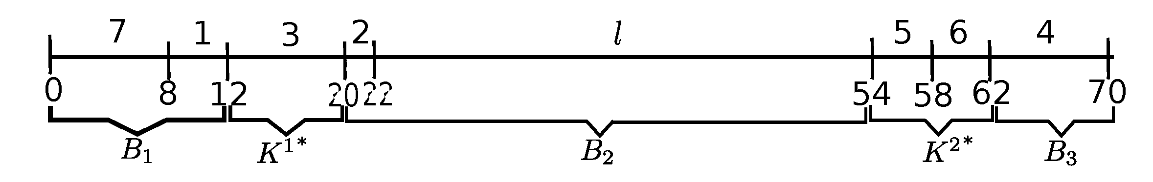
In general, we have a bin between two adjacent kernel intervals, and a bin before the first and after the last kernel interval. Because of the allowable right-shift for the jobs of an atomic kernel , the starting and completion times of the corresponding kernel and bin intervals are not priory fixed. We denote by (, respectively) the bin before (after, respectively) the kernel interval corresponding to the atomic kernel of kernel K. There are two bins in schedule , surrounding the atomic kernel consisting of Job 1 in Figure 6. We have three bins in schedules depicted in Figure 8 and Figure 9 for the problem instance of Example 2, , and (schedule of Figure 9 incorporates an optimal arrangement of jobs in these bins).
The scope of augmented L-schedule for kernel K includes that of bin and that of the atomic kernel . These two parts are scheduled independently. The construction of second part relies on the next proposition that easily follows from Proposition 9:
Proposition 10.
No job of the atomic kernel will surpass the L-boundary if the latest scheduled job of bin completes no later than at time moment
(the latest time moment when atomic kernel may start in an L-schedule) and the jobs of that kernel are scheduled by ED-heuristics from time moment .
We easily arrange the second part of augmented schedule , i.e., one including the atomic kernel , as specified in Proposition 10. Hence, from here on, we are solely concerned with the construction of the the first part, i.e., that of bin , which is a complicated task and basically contributes to the complexity status of problem .
We refer to a partial feasible L-schedule for the first part of schedule (with its latest job completion time not exceeding the magnitude , at which the second part initiates) as a preschedule of kernel K and denote it by . Note that the time interval of preschedule coincides with that of bin ; in this sense, is a schedule for bin .
Kernel preschedules are generated in Phase 1, described in Section 7. If Phase 1 fails to construct an L-preschedule for some kernel, then Phase 2 described in Section 9 is invoked (see Proposition 12 in Section 5). Phase 2 basically uses the construction procedure of Phase 1 for the new problem instances that it derives.
6.1.1. The Main Partitioning Procedure
Now, we describe the main procedure (PROCEDURE MAIN) of our algorithm, that is in charge of the partitioning of the scheduling horizon into the kernel and the corresponding bin intervals. This partition is dynamically changed and is updated in a recurrent fashion each time a new kernel arises. The occurrence of each new kernel K during the construction of a bin, the split of this bin into smaller bins and the collapsing of kernel K induce the recurrent nature in our method (not surprising, the recurrence is a common feature in the most common algorithmic frameworks such are dynamic programming and branch-and-bound).
Invoked for kernel K (K is a global variable), PROCEDURE MAIN first calls PROCEDURE Decomposition that forms schedule ending with the atomic kernel (see the beginning of Section 5 and Propositions 5 and 9).
PROCEDURE MAIN incorporates properly kernel K into the current partition updating respectively the current configuration defined by a trial , the current set of kernels together with the corresponding s (see Equation (7)) and the augmented schedules , for , constructed so far.
Given trial and kernel K, the configuration is unique, and there is a unique corresponding schedule with that includes the latest generated (so far) augmented schedules , .
PROCEDURE MAIN starts with the initial configuration with , , and (no bin exists yet in that configuration).
Iteratively, PROCEDURE MAIN, invoked for kernel K, creates a new configuration with two new surrounding bins and and the atomic kernel in between these bins. These bins arise within a bin of the previous configuration (the later bin disappears in the updated configuration). Initially, atomic kernel splits schedule in two bins and .
Two (atomic) kernels in schedule are tied if they belong to the same block in that schedule.
Given configuration , the longest sequence of the augmented L-schedules of the pairwise tied kernels in schedule is called a secondary block.
We basically deal with the secondary block containing kernel K and denote it by (we may omit argument K when this is not important). An essential characteristic of a secondary block is that every job that pushes a job from that secondary block belongs to the same secondary block. Therefore, the configuration update in PROCEDURE MAIN can be carried out solely within the current secondary block .
As we show below, PROCEDURE MAIN will create an L-schedule for an instance of whenever it exists (otherwise, it affirms that no L-schedule for that instance exists). The same outcome is not guaranteed for an instance of , in general. In Theorem 3, we give an explicit condition under which an L-schedule for an instance of will always be created, yielding a polynomial-time solution for the general setting. Unfortunately, if the above condition is not satisfied, we cannot, in general, affirm that there exists no feasible L-augmented schedule, even if our framework fails to find it for an instance of problem .
6.1.2. PROCEDURE AUGMENTED , Rise of New Kernels and Bin Split
PROCEDURE MAIN uses PROCEDURE AUGMENTED as a subroutine. PROCEDURE AUGMENTED, called for kernel K with threshold , is in charge of the creation of an -augmented schedule respecting the current configuration . PROCEDURE AUGMENTED constructs the second part of schedule (one including the atomic kernel ) directly as specified in Proposition 10. The most time consuming part of PROCEDURE AUGMENTED is that of the construction of the preschedule of schedule . This construction is carried out at Phase 1 described in Section 7.
After a call of PROCEDURE AUGMENTED, during the construction of an L-preschedule at Phase 1, a new kernel may arise (the reader may have a look at Proposition 12 and Lemma 5 from the next section). Then, PROCEDURE AUGMENTED returns the newly arisen kernel and PROCEDURE MAIN, invoked for that kernel, updates the current configuration. Since the rise of kernel splits the earlier bin into two new surrounding bins and of the new configuration, the bin of the previous configuration disappears and is “replaced” by a new bin of the new configuration. Correspondingly, the scope of a preschedule for kernel K is narrowed (the former bin is “reduced” to the newly arisen bin ).
In this way, as a result of the rise of a new kernel within the (current) bin and the resultant bin split, PROCEDURE AUGMENTED may be called more than once for different (gradually decreasing in size) bins: The initial bin splits into two bins, the resultant new smaller bin may again be split, and so on. Thus, to the first call of PROCEDURE AUGMENTED the largest bin corresponds, and the interval of the new arisen bin for every next call of the procedure is a proper sub-interval of that of the bin corresponding to the previous call of the procedure. Note that each next created preschedule is composed of the jobs from the corresponding bin.
PROCEDURE AUGMENTED has three outcomes. If no new kernel during the construction of preschedule respecting the current configuration arises, the procedure completes with the successful outcome generating an L-augmented schedule respecting the current configuration (in this case, schedule may form part of the complete L-augmented schedule if the later schedule exists). PROCEDURE MAIN incorporates -augmented schedule into the current configuration (the first IF statement in the iterative step in the description of the next subsection).
With the second outcome, a new kernel during the construction of preschedule within bin arises (Proposition 12 and Lemma 5). Then, PROCEDURE AUGMENTED returns kernel and PROCEDURE MAIN is invoked for this newly arisen kernel and it updates the current configuration, respectively (see the iterative step in the description). Then, PROCEDURE MAIN calls recursively PROCEDURE AUGMENTED for kernel and the corresponding newly arisen bin (this call is now in charge of the generation of an L-preschedule for kernel , see the second IF statement in the iterative step of the description in the next subsection).
With the third (failure) outcome, Phase 1 (invoked by PROCEDURE AUGMENTED for the creation of an L-preschedule ) fails to create an L-preschedule respecting the current configuration (an IA(b2), defined in the next section, occurs (see Proposition 12). In this case, PROCEDURE MAIN invokes Phase 2. Phase 2 is described in Section 9. Nevertheless, the reader can see a brief description of that phase below:
Phase 2 uses two subroutines, PROCEDURE sl-SUBSTITUTION and PROCEDURE ACTIVATE, where s is an emerging job. PROCEDURE sl-SUBSTITUTION generates modified configurations with an attempt to create an L-preschedule respecting a newly created configuration, in which some preschedules of the kernels, preceding kernel K in the secondary block are reconstructed. These preschedules are reconstructed by the procedure of Phase 1, which is called by PROCEDURE ACTIVATE. PROCEDURE ACTIVATE, in turn, is repeatedly called by PROCEDURE sl-SUBSTITUTION for different emerging jobs in the search of a proper configuration (each call of PROCEDURE ACTIVATE creates a new configuration by a call of Phase 1). If at Phase 2 a configuration is generated for which Phase 1 succeeds to create an L-preschedule respecting that configuration (the successful outcome), the augmented L-schedules corresponding to the reconstructed preschedules remain incorporated into the current schedule .
6.1.3. Formal Description of PROCEDURE MAIN
The formal description of PROCEDURE MAIN below is completed by the descriptions of Phases 1 and 2 in the following sections. For notation simplicity, in set operations, we use schedule notation for the corresponding set of jobs. Given a set of jobs A, we denote by the ED-schedule obtained by the application of ED-heuristics to the jobs of set A.
Whenever a call of PROCEDURE MAIN for kernel K creates an augmented L-schedule , the procedure completes secondary block by merely applying ED-heuristics to the remaining available jobs, ones to be included in that secondary block; i.e., partial ED-schedule is generated and is merged with the already created part of block to complete the block (the rest of the secondary blocks are left untouched in the updated schedule ).
PROCEDURE MAIN returns -schedule with the minimal , which is optimal by Lemma 8.
PROCEDURE MAIN
Initial step: {Determine the initial configuration , }
Start the binary search with trial
{initialize the set of kernels}
;
{set the initial lower bound and the initial allowable delay for kernel K}
);
IF schedule contains no kernel with the delaying emerging job, output and halt
{ is optimal by Proposition 1}
Iterative step:
{Update the current configuration with schedule as follows:}
{update the current set of kernels}
;
{update the current lower bound}
;
{update the corresponding allowable kernel delays (see Equation (7))}
, for every kernel
Call PROCEDURE AUGMENTED {construct an -augmented schedule }
IF during the execution of PROCEDURE AUGMENTED a new kernel arises
{update the current configuration according to the newly arisen kernel}
THEN ; repeat Iterative step
IF the outcome of PROCEDURE AUGMENTED is failure THEN call Phase 2
{at Phase 2 new configuration is looked for such that there exist preschedule respecting that configuration, see Section 9}
IF -augmented schedule is successfully created
{the outcome of PROCEDURE AUGMENTED and that of Phase 2 is successful, hence complete secondary block by ED-heuristics if there are available jobs which were not included in any of the constructed augmented schedules, i.e., }
THEN update block and schedule by merging it with partial ED-schedule
(leave in the updated schedule the rest of the secondary blocks as they are)
IF (the so updated) schedule is an -schedule
{continue the binary search with the next trial }
THEN the next trial value and repeat Iterative step; return the generated -schedule with the
minimum and halt if all the trial s were already considered
ELSE {there is a kernel with the delaying emerging job in schedule }
; repeat Iterative step
IF -augmented schedule could not been created
{the outcome of Phase 2 is failure and hence there exists no -schedule; continue the binary search with the next trial }
THEN the next trial value and repeat Iterative step; return the generated -schedule with the
minimum and halt if all the trial s were already considered.
7. Construction of Kernel Preschedules at Phase 1
At Phase 1, we distinguish two basic types of the available (yet unscheduled) jobs which can feasibly be included in bin , for every . Given a current configuration, we call jobs that can only be scheduled within bin y-jobs; we call jobs which can also be scheduled within some succeeding bin(s) the x-jobs for bin or for kernel K. In this context, y-jobs have higher priority.
We have two different types of the y-jobs for bin . The set of the Type (a) y-jobs is formed by the jobs in set and yet unscheduled jobs not from kernel K released within the interval of bin . The rest of the y-jobs are ones released before the interval of bin , and they are referred to as the Type (b) y-jobs.
Recall that the interval of bin begins right after the atomic kernel of the preceding bin (or at if K is the earliest kernel in ) and ends with the interval of schedule . The following proposition immediately follows:
Proposition 11.
Every x-job for bin is an external job for kernel K, and there may also exist the external y-jobs for that kernel. A Type (a) y-job can feasibly be scheduled only within bin , whereas Type (b) y-jobs can potentially be scheduled within a preceding bin (as they are released before the interval of bin ).
Phase 1 for the construction of preschedule of kernel K consists of two passes. In Pass 1 y-jobs of bin are scheduled. In Pass 2, x-jobs of bin are distributed within that bin. We know that all Type (a) y-jobs can be feasibly scheduled within bin without surpassing the L-boundary (since they were so scheduled in that bin), and these jobs may only be feasibly scheduled within that bin. Note that, respecting the current configuration with the already created augmented schedules for the kernels in set ), we are forced to include, besides Type (a) y-jobs, also all the Type (b) y-jobs into bin . If this does not work at Phase 1 in the current configuration, we try to reschedule some Type (b) y-jobs to the earlier bins in Phase 2 by changing the configuration.
7.1. Pass 1
Pass 1 consists of two steps. In Step 1, ED-heuristics is merely applied to all the y-jobs for scheduling bin .
If the resultant ED-schedule is a feasible L-schedule (i.e., no job in it surpasses the current L-boundary and/or finishes after time ), Step 1 completes with the successful outcome and Pass 1 outputs (in this case, there is no need in Step 2), and Phase 1 continues with Pass 2 that augments with x-jobs, as described in the next subsection.
If schedule is not an L-schedule (there is a y-job in that schedule surpassing the L-boundary), Pass 1 continues with Step 2.
Proposition 12 specifies two possible cases when preschedule does not contain all the y-jobs for bin , and Step 1 fails to create an L-preschedule for kernel K at the current configuration.
Proposition 12.
Suppose is not a feasible L-schedule, i.e., there arises a y-job surpassing the current L-boundary and/or completing after time .
(1) If there is a Type (b) y-job surpassing the L-boundary, then there exists no feasible partial L-preschedule for kernel K containing all the Type (b) y-jobs for this kernel (hence there is no complete feasible L-schedule respecting the current configuration).
(2) If there is a Type (a) y-job y surpassing the L-boundary and there exists a feasible partial L-preschedule for kernel K containing all the y-jobs, it contains a new kernel consisting of some Type (a) y-jobs including job y.
Proof.
We first show Case (2). As already mentioned, all Type (a) y-jobs may potentially be included in bin without surpassing the L-boundary and be completed by time (recall Equation (12)). Hence, since y is a Type (a) y-job, it should have been pushed by at least one y-job i with in preschedule . Then, there exists the corresponding kernel with the delaying emerging y-job (containing job y and possibly other Type (a) y-jobs).
Now, we prove Case (1). Let y be a Type (b) y-job that was forced to surpass the L-boundary and/or could not be completed by time moment . In the latter case, ED-heuristics could create no gap in preschedule as all the Type (b) y-jobs were released from the beginning of the construction, and Case (1) obviously follows. In the former case, job y is clearly pushed by either another Type (b) y-job or a Type (a) y-job. Let k be a job pushing job y. Independently of whether k is a Type (a) or Type (b) y-job, since job y is released from the beginning of the construction and job k was included ahead job y, by ED-heuristics, . Then, no emerging job for job y may exist in preschedule and Case (1) again follows as all the Type (a) y-jobs must be included before time . □
For convenience, we refer to Case (1) in Proposition 12 as an instance of Alternative (b2) (IA(b2) for short) with Type (b) y-job y (we let y be the latest Type (b) y-job surpassing the L-boundary and/or completing after time ). (The behavior alternatives were introduced in a wider context earlier in [13].) If an IA(b2) in bin arises and there exists a complete L-schedule, then, in that schedule, some Type (b) y-job(s) from bin is (are) included within the interval of some bin(s) preceding bin in the current secondary block (we prove this in Proposition 16 in Section 7).
In Step 2, Cases (1) and (2) are dealt with as follows. For Case (1) (an IA(b2)), Step 2 invokes PROCEDURE sl-SUBSTITUTION of Phase 2. PROCEDURE sl-SUBSTITUTION creates one or more new (temporary) configurations, as described in Section 7. For every created configuration, it reconstructs some bins, preceding bin in the secondary block incorporating some Type (b) y-jobs for bin into the reconstructed preschedules. The purpose of this is to find out if there exists an L-preschedule respecting the current configuration and construct it if it exists.
For Case (2) in Proposition 12, Step 2 returns the newly arisen kernel and PROCEDURE MAIN is invoked with that kernel, which updates the current configuration respectively. PROCEDURE MAIN then returns the call to PROCEDURE AUGMENTED (see the description of Section 4) (note that, since PROCEDURE AUGMENTED invokes Phase 1 now, for kernel , Case (2) yields recursive calls of Phase 1).
7.2. Pass 2: DEF-Heuristics
If Pass 1 successfully completes, i.e., creates a feasible L-preschedule , Pass 2, described in this subsection, is invoked (otherwise, IA(b2) with a Type (b) y-job from bin arises and Phase 2 is invoked). Throughout this section, stands for the output of Pass 1 containing all the y-jobs for bin . At Pass 2, the x-jobs released within the remaining available room in preschedule are included by a variation of the Next Fit Decreasing heuristics, adopted for our scheduling problem with job release times. We call this variation Decreasing Earliest Fit heuristics, DEF-heuristics for short. It works with a list of x-jobs for kernel K sorted in non-increasing order of their processing times, the ties being broken by sorting jobs with the same processing time in the non-decreasing order of their due-dates.
DEF-heuristics, iteratively, selects next job x from the list and initially appends this job to the current schedule by scheduling it at the earliest idle-time moment before time (any unoccupied time interval in bin before time is an idle-time interval in that bin). Let be the resultant partial schedule, that is obtained by the application of ED-heuristics from time moment to job x and to the following y-jobs from schedule which may possibly right-shifted in schedule ) (compared to their positions in schedule ). In the description below, the assignment updates the current partial schedule according to the rearrangement in schedule , removes job x from the list and assigns to variable x the next x-job from the list.
PROCEDURE DEF()
IF job x completes before or at time in schedule {i.e., falls within the current bin}
THEN GO TO Step (A) {verify the conditions in Steps (A) and (B)}
ELSE remove job x from the list {job x is ignored for bin }; set x to the next job from the list;
CALL PROCEDURE DEF()
(A) IF job x does not push any y-job in schedule {x can be scheduled at time moment without the interference with any y-job, i.e., is no greater than the starting time of the next y-job in preschedule } and it completes by time moment in schedule
THEN ; CALL PROCEDURE DEF()
(B) IF job x pushes some y-job in schedule
THEN {verify the conditions in Steps (B.1)–(B.3)}
(B.1) IF in schedule no (right-shifted) y-job surpasses L-boundary and
all the jobs are completed by time moment
THEN ; CALL PROCEDURE DEF()
(B.2) IF in schedule some y-job completes after time moment
THEN set x to the next x-job from the list and CALL PROCEDURE DEF().
We need the following auxiliary lemma before we describe Step (B.3):
Lemma 5.
If a (right-shifted) y-job surpasses L-boundary in schedule , then there arises a new kernel in that schedule (in bin ) consisting of solely Type (a) y-jobs, and x is the delaying emerging job of that kernel.
Proof.
Obviously, by the condition in the lemma, there arises a new kernel in schedule , call it , and it consists of y-jobs following job x in schedule . Clearly, x is the delaying emerging job of kernel . Such a right-shifted job y cannot be of Type (b) as otherwise it would have been included within the idle-time interval (occupied by job x) at Pass 1. Hence, kernel consists of only Type (a) y-jobs. □
Due to the above lemma, PROCEDURE DEF continues as follows:
(B.3) IF in schedule the lateness of some (right-shifted) y-job exceeds L
THEN return the newly arisen kernel and invoke PROCEDURE MAIN with kernel {this updates the current configuration respectively and makes a recursive call of Phase 1 now for kernel }
IF the list is empty THEN OUTPUT() and halt.
This completes the description of Pass 2 and that of Phase 1.
From here on, we let be the output of Phase 1 (a feasible L-preschedule for kernel K containing all the y-jobs for bin ). An easily seen property of PROCEDURE DEF and preschedule is summarized in the following proposition.
Proposition 13.
An L-preschedule cannot be obtained by replacing any x-job with a longer available x-job in preschedule . Hence, the omission of job x from preschedule will create a new gap which may only be filled in by including job(s) with the same or smaller processing time.
Let and be the number of y-jobs and x-jobs of bin , respectively, is the total number of jobs in that bin, and let be the number of Type (b) y-jobs. The next theorem gives a valid upper bound on the cost of a call of PROCEDURE AUGMENTED at Phase 1 (including all the recursive calls that the initial call may yield).
Theorem 2.
The total cost of a call of Phase 1 for a kernel K is . Hence, the cost of a call of PROCEDURE AUGMENTED is the same.
Proof.
At Step 1 of Pass 1, during the construction of preschedule ED-heuristics with an upper bound on its running time for scheduling up to y-jobs is used, whereas at less than scheduling times a new kernel may arise (as the delaying emerging job may only be a Type (b) y-job). Phase 1 invokes PROCEDURE MAIN which, in turn, calls the decomposition procedure for each of these kernels. By Lemma 2, the total cost of all the calls of the decomposition procedure can be estimated as , where is the number of jobs in each of the arisen kernels, correspondingly. Let m be the mean arithmetic of all these s. Since any newly arisen kernel may contain only y-jobs for bin and no two kernels may have a common job, . The maximum in the sum is reached when all the s are equal to m, and from the above sum another no-smaller magnitude is obtained (in the first and second inequalities, and , respectively, are applied).
Then, the total cost of Pass 1 for kernel K (including that of Step 2, Case (2)) is . The cost of Steps (A), (B.1) and (B.2) of Pass 2 is that of ED-heuristics, i.e., . At Step (B.3), since the delaying emerging job for every newly arisen kernel is a distinct x-job for bin , the number of the calls of PROCEDURE MAIN for all the newly arisen kernels after the initial call of PROCEDURE AUGMENTED, and hence the number of the recursive calls of Phase 1 for kernel K, is bounded by . Similar to what is done for Pass 1, we let be the number of jobs in each of the arisen kernels, respectively. Again, by Lemma 2, the total cost of all the calls of PROCEDURE MAIN to the decomposition procedure is . We let again m be the mean arithmetic of all these s, and obtain an upper bound on the cost of Pass 2 and hence the total cost of Phase 1 is .
The second claim in theorem follows as the cost of the generation of the second part of an augmented -schedule is absorbed by that of the first part. Indeed, recall that for a call of PROCEDURE AUGMENTED, the second part of schedule consisting of the jobs of the atomic kernel , is constructed by ED-heuristics in time , where is the total number of jobs in atomic kernel , and is the number of jobs in kernel K (Proposition 10). Similar to above in this proof, we can show that the construction of the second part of the augmented schedules for the calls of PROCEDURE AUGMENTED for all the arisen kernels (for the same ) is . □
At this stage, we can give an optimality (sufficient) condition for problem , that is helpful also in that it exhibits where the complex nature of the problem is “hidden”. Dealing with an IA(b2) is a complicated task as it implies the solution of NP-hard set/numerical problems such as 3-PARTITION yet with additional restrictions that impose job release times. As to the solution provided by PROCEDURE MAIN, as we have seen above, the recurrences at Step 2, Case (2) in Pass 1, and at Step (B.3) at Pass 2 do not, in fact, cause an exponential behavior.
Theorem 3.
PROCEDURE MAIN finds an optimal solution to problem in time if no IA(b2) at Phase 1 arises.
Proof.
The proof is quite straightforward, we give a scratch. The initial step takes time (the cost of ED-heuristics). At iterative step, the cost of updates of and , and that of the detection of every newly arisen kernel is bounded by the same magnitude. It is easy to see that an L-preschedule for every kernel in will be generated at Phase 1 if no Type (b) y-job is forced to surpasses the L-boundary, or, equivalently, no IA(b2) arises (only a y-job may be forced to surpass the L-boundary, whereas, if a Type (a) y-job surpasses it, PROCEDURE MAIN proceeds with the newly arisen kernel). Hence, PROCEDURE AUGMENTED will create a feasible L-augmented schedule for every kernel (since no IA(b2) at Pass 1 arises). Then, it remains to estimate the calls of PROCEDURE AUGMENTED in the iterative step. The cost of a call of PROCEDURE AUGMENTED for a given kernel K including all the embedded recursive calls is (Theorem 2). These recursive calls include the calls for all the kernels which may arise within bin . Hence, for the purpose of our estimation, it suffices to distinguish the calls PROCEDURE AUGMENTED and PROCEDURE AUGMENTED for two distinct kernels K and M such that bins and have no jobs in common. Then, similar to what is done to estimate the cost of Pass 1 in the proof of Theorem 2, we easily get an overall (amortized) cost of for PROCEDURE MAIN for a given trial . Then, we obtain the overall cost of for PROCEDURE MAIN taking into account that there are no more than trial s. □
8. Construction of Compact Preschedules for Problem
This section starts Part 2, in which our basic task is to develop an auxiliary algorithm that deals with an IA(b2) occurred at Phase 1 (recall that if no IA(b2) occurs, PROCEDURE MAIN with PROCEDURE AUGMENTED using Phase 1 already solves problem ). A compact feasible schedule, one without any redundant gap, has properties that are helpful for the establishment of the existence or the non-existence of a complete L-schedule whenever during the construction of a kernel preschedule at Phase 1 an instance of Alternative (b2) arises. In this section, we study the compactness properties for instances of problem .
Since the basic construction components of a complete feasible schedule are the secondary blocks, it suffices to deal with compact secondary blocks. A secondary block is compact if there is no feasible L-schedule containing all the jobs of that block with the total length of all the gaps in it no-less than that in block .
We can keep the secondary blocks compact if the processing times of some non-kernel jobs are mutually divisible. For the commodity and without loss of generality, we assume that the processing times of the non-kernel jobs are powers of 2 (precisely, we identify the specific non-kernel jobs for which mutual divisibility is required on the fly). Below, we give a basic property of a set of divisible numbers and then we give another useful property of a kernel preschedule with divisible job processing times, which are used afterwards.
Lemma 6.
For a given job x, let be the set of jobs such that and the processing times of jobs in set are mutually divisible. Then, there exists a proper subset of set with (that can be found in an almost liner time).
Proof.
The following simple procedure finds subset . Sort the jobs in set in non-increasing order of their processing times, say . It is straightforward to see that, because of the divisibility of the processing times of the jobs in set , there exists integer such that , i.e., . □
Lemma 7.
Preschedule , constructed at Pass 2 of Phase 1 for an instance of , contains no gap except one that may possibly arise immediately before time moment .
Proof.
By the way of contradiction, suppose I is an internal gap in schedule of Pass 1. Note that initially, gap I was completely occupied in bin in schedule , and that it is succeeded by at least one y-job in preschedule . That is, the x-jobs with the total length of at least should have been available while scheduling the interval of gap I in PROCEDURE DEF at Pass 2. Then, an idle time interval within the interval of gap I in preschedule of Pass 2 may potentially occur only at the end of that interval, say at time moment , due to the non-permitted interference in schedule of an available (and not yet discarded) x-job with a succeeding y-job, say y (Step (B)). Note that job y is a Type (a) y-job (if it were of Type (b), then it would have been included ahead any x-job in bin ) and that the lateness of that job did not exceed L before kernel K was detected in schedule . Let X be the set of the x-jobs preceding job y in the interval of gap I in the latter schedule, and be the corresponding set of the x-jobs in preschedule (by our construction, ). In PROCEDURE DEF, during the construction of schedule , at time moment there must have been no job with processing time or less available. However, this is not possible since, because of the divisibility of job processing times, set X must contain such a job (and that job must have been available and yet unscheduled). The existence of a gap from time moment in the interval of gap I in schedule has led to a contradiction and hence it cannot exist. □
In the rest of this section, we assume that preschedule contains a gap; i.e., it ends with a gap (Lemma 7). Our objective is to verify if that gap can be reduced. To this end, we define two kinds of jobs such that their interchange may possibly be beneficial.
The first type of jobs are formed from set , the set of the passive emerging jobs for kernel K in the current configuration with threshold . Recall that a job from set is included after kernel K in schedule but it may feasibly be included (as an x-job) in a preschedule of kernel K (in bin ).
Recall at the same time, that a job from preschedule which may be rescheduled after all jobs of kernel K without surpassing the L-boundary is one from set , the set of emerging jobs for kernel K at the current configuration (such a job was included as an x-job in preschedule ).
A vulnerable component of a secondary block is a preschedule in it, in the sense that we can maintain a secondary block compact if every preschedule that it contains is also compact, i.e., there exists no other preschedule (for the same kernel) with the total length of the gaps less than that in the former preschedule (see Corollary 4 at the end of this section). A key informal observation here is that, if a preschedule for kernel K is not compact, then a compact one can only be obtained from the former preschedule by replacing some jobs from set with some jobs from set , whereas nothing is to be gained by substituting any jobs from a compact preschedule by any jobs from set (Proposition 14 below).
Let and . Consider A and B as potential “swap” subsets and denote by the preschedule for kernel K obtained by interchanging the roles of jobs from sets A and B while reconstructing the current preschedule by the procedure of Phase 1. Technically, preschedule can be constructed at Phase 1 for the restricted problem instance PI that contains all jobs from preschedule and set B but does not contain ones in set A (so jobs from set A are activated for kernel K). Note that a job from set A belongs to , and, along with the remaining jobs from preschedule , some job(s) from set B may also be included in .
Proposition 14.
If an L-preschedule is not compact then there exist sets A and B such that an L-preschedule is compact.
Proof.
Among the jobs included in schedule after preschedule , the available room (the gap) from preschedule may only potentially be used by job(s) from set . By the construction of Phase 1, this will not be possible unless some emerging job(s) from preschedule is (are) rescheduled after kernel K. Then, this kind of the interchange of the jobs from set with the jobs from set yields the only potentially improving rearrangement of the jobs in preschedule , and the proposition follows. □
Let us say that set Acovers set B if preschedule includes all jobs from problem instance PI. Since we wish to reduce the total gap length in preschedule , must hold, which is our assumption from now on (we use for the total processing time in job-set A; below, we use for the minimum job processing time in A).
Let the total gap length in preschedule . We call
the store of kernel K in the current configuration . It is easily seen that is the maximum available vacant room in preschedule :
Proposition 15.
The total length of the jobs (the gaps, respectively) in preschedule might be increased (decreased, respectively) by at most time units in any L-preschedule for kernel K. If set A covers set B, then the store of kernel K in an updated configuration with preschedule is
Lemma 8.
If , then preschedule is compact. If preschedule is not compact, then , for any .
Proof.
By the condition in lemma, the gap in preschedule (see Lemma 7) can potentially be occupied only by a job j with (see Proposition 15). There may exist no such job in set as otherwise it would have been included in preschedule as an x-job at Pass 2. Now, it can be straightforwardly seen that no interchange of jobs in set from preschedule with jobs from set may reduce the gap, because of the divisibility of the processing times of the jobs in sets and , and the first claim in lemma follows from Proposition 14.
Now, we show the second claim. Suppose preschedule is not compact. Then, there exist sets A and B such that A covers B and preschedule results in the reduction of the store of kernel K by (see Equation (13) and Propositions 14 and 15). Because of the divisibility of job processing times in sets A and B, is a multiple of . Hence, if , then preschedule is compact; must hold if is not compact. is not possible, as otherwise a job from set B with processing time would have been included in preschedule at Pass 2 of Phase 1. It follows that . □
Due to Lemma 8, from here on, assume that . It is not difficult to see that not all time units may potentially be useful. In particular, let be the maximum integer such that , and let .
Lemma 9.
A feasible L-preschedule contains gap(s) with the total length of at least ; hence, when set A covers set B. Furthermore, , for some integer , and .
Proof.
The first claim easily follows from the definitions and the mutual divisibility of the processing times of jobs in sets A and B, and inequality immediately follows. As to the second claim, first we note that, for any , , as otherwise job would have been included in preschedule at Pass 2 of Phase 1. Then, , whereas . Hence, . Now, the second claim follows from the fact that the processing times of jobs in sets and A are powers of 2. □
Example 3.
Suppose and . Then, , hence a gap of length 3 is unavoidable. Let . Since the shortest job that set B may contain has processing time 32, the most we may expect is to form set A of three jobs of (the minimal) length 4, set B being formed by a single job with the length 32. Then, after swapping sets A and B, we have a residue . Because of these extra 20 units, the available idle space of length 23 is reduced to 3 in schedule in which set A covers set B. In that schedule, a gap of (the minimal possible) length occurs.
We may restrict our attention to sets A and B which do not contain equal-length jobs, as otherwise we may simply discount the corresponding jobs from both sets. In particular, for given A and B with and with , we obtain sets and by eliminating job i and job j, respectively, from sets A and B, respectively. Let and be the reduced sets A and B, respectively, obtained by the repeated application of the above operation for all equal-length jobs. Sets and contain no equal-length jobs. We have proved the following lemma.
Lemma 10.
If set A covers set B, then set covers set , where .
Theorem 4.
If set A covers set B, then there are also (reduced) sets and , where set contains a single element with the minimum processing time in set B and with such that set covers set and .
Proof.
Let A and B be the reduced sets that contain no equal-length jobs and such that A covers B (see Lemma 10). We can further reduce sets A and B by discounting, similarly, for each job , jobs from set A, for which processing times sum up to . In particular, take a longest job and longest jobs from set A that sum up to . Due to the divisibility of job processing times and the inequalities and (see Lemma 9), this will be possible as long as the total processing time in A is no smaller than . The sets A and B are reduced respectively, and the same operation for these reduced sets is repeated until the total processing time of the remaining jobs in the reduced set A is less than . Then, we are left with a single job (one with the minimum processing time in B) and the jobs in set A with the total processing time less than , and such that (see Lemma 9).
Let and be the reduced sets obtained from sets A and B, respectively. By the construction of set and and the fact that set A covers set B, it immediately follows that and that set covers set . □
Now, we show that the current secondary block will be kept compact if we merely unify the compact preschedules in schedule .
Theorem 5.
A secondary block consisting of compact L-preschedules is compact.
Proof.
If the time interval of every preschedule from block extends up to time and it contains no gap then the secondary block is clearly compact. Suppose there is preschedule from block that contains a gap and/or completes before time . First, we observe that no extra job can be included within preschedule to obtain another L-preschedule with an extended time interval and/or with less total gap length. Indeed, let , , be a shortest available x-job from set . By PROCEDURE DEF, schedule is not a feasible L-preschedule for kernel K (as otherwise PROCEDURE DEF would include job in preschedule at Pass 2). Thus, job may only feasibly be included in preschedule by removing a longer job x from that preschedule. However, such a rearrangement may, at most, fill in the former execution interval of job x due to the above made observation and Lemma 6.
To prove the lemma, now it clearly suffices to show that nothing is to be gained by a job rearrangement in preschedule that involves, besides the jobs from sets and , the jobs from a preschedule preceding preschedule .
Let be an arbitrary L-preschedule for kernel K (one respecting the current threshold ). Without loss of generality, assume preschedules and start at the same time, whereas none of them may complete after time (Equation (12)). Let W and Z, respectively, be the sets of integer numbers, the processing times of jobs in the current preschedule and in preschedule , respectively (here, we assume that sets W and Z consist of mutually divisible integer numbers, possibly with some repetitions).
Similar to what is done in Lemma 10 and Theorem 4, we discount the same numbers from sets W and Z and the numbers from one set which sum up to another number from the other set (taking a combination with the longest possible jobs). Note that both sets are reduced by the same amount (a sum of powers of 2). Denote by and the resultant sets.
If then the total gap length in preschedule cannot be more than that in preschedule , and the theorem follows if the condition holds for all preschedules in block .
Otherwise, suppose . By the definition of the sets and and the store of kernel K (Equation (13)), (see Theorem 4) and the preschedule for kernel K consisting of the jobs associated with the set of processing times will have the same total gap length as preschedule (the substitution of the jobs corresponding to set by those from set would result in a preschedule with the same total gap length as that in preschedule ). By the construction of preschedule at Phase 1, no job x with processing time from set which could have been feasibly included within preschedule was available during the construction of that preschedule. Hence, every such job x should have been already scheduled in a preschedule preceding preschedule in block . By rescheduling job x from preschedule to preschedule , the total gap length in the newly created preschedule of kernel K will be reduced by , but a new gap of the same length will occur in the resultant new preschedule of kernel as there is no other suitable job available (otherwise, it would have been included in preschedule ). Hence, the total gap length in block will remain the same. Thus, no matter how the jobs are redistributed among the preschedules from block , the total length of the remaining gaps in that block will remain the same. The lemma is proved. □
Corollary 4.
If a secondary block is constituted by the preschedules created at Phase 1, then it is compact.
Proof.
For every kernel , if an L-preschedule of Phase 1 is not compact then there exist sets and such that an L-preschedule is compact (Proposition 14). By Theorem 4, , for some job . However, since for every job , (see Lemma 9), set A cannot cover set B in preschedule , as otherwise job would have been included in preschedule at Pass 2 instead of the shorter jobs from set A. It follows that every preschedule from block is compact, and the corollary follows from Theorem 5. □
9. Phase 2: Search for an L-preschedule When an IA(b2) at Phase 1 Arises
Throughout this section, we consider the scenario when a compact preschedule for a newly arisen kernel K cannot be constructed at Phase 1, i.e., an IA(b2) with a Type (b) y-job y at Pass 1 arises. Recall that this happens when Pass 1 is unable to include job y in preschedule in the current configuration (see Proposition 12). Phase 2, invoked from Phase 1, generates one or more new problem instances and calls back Phase 1 to create the corresponding new configurations. Thus, Phase 2 has no proper algorithmic features except that it generates new problem instances.
We refer to the earliest occurrence of IA(b2) in secondary block at Phase 1 as the basic case. In the inductive case (abbreviated IA(b2-I)), IA(b2) repeatedly arises in the current secondary block (roughly, we “stay” in the current secondary block for IA(b2-I) in the inductive case, whereas we are brought to a new secondary block with every newly occurred IA(b2) in the basic case). In general, different occurrences of an IA(b2-I) in the inductive case may occur for different kernels, where all of them pertain to the current secondary block .
Throughout this section, let be the kernel immediately preceding kernel K in block . We let y be an incoming job in bin at Phase 1; y is an incoming job in the first bin of block if there exists no . Note that is no smaller than the starting time of block , and, since it can feasibly be scheduled within every bin that initiates at or after time up to (and including) bin , y is a former x-job for any such a bin (except that it is a Type (b) job for bin ), i.e., it may potentially be included in any of these bins. We explore such possibility and seek for a suitable distribution of all the x-jobs and Type (b) y-jobs into these bins at Phase 2.
Proposition 16.
Suppose during the construction of preschedule an IA(b2)/IA(b2-I) with job y occurs and there exists schedule . Then, job y or a Type (b) y-job included between kernel and job y in bin is scheduled before kernel in schedule .
Proof.
Note that the critical block in schedule coincides with the secondary block , and it is compact when the above IA(b2)/IA(b2-I) occurs by Corollary 4. Then, job y cannot be restarted earlier in any feasible L-schedule in which the same jobs (which were included in preschedule at Pass 1) are left scheduled before job y. The lemma obviously follows if y is the earliest considered job to be scheduled in bin . Otherwise, job y may potentially be started earlier either by scheduling it before kernel or by decreasing (left-shifting) its current early starting time. The latter will only be possible if some job included in bin ahead of job y is rescheduled behind job y. By the construction at Phase 1, any job included in bin ahead of job y is a no less urgent than job y y-job and it cannot be rescheduled after job y without surpassing the L-boundary. Then, job y may be left-shifted only if one of the latter jobs is rescheduled before kernel . However, this is not possible for a Type (a) y-job and the lemma is proved. □
By the above proposition, either job y or a Type (b) y-job included between kernel and job y in bin is to be rescheduled before kernel . In particular, the following observations are evident:
- (1) If job y, is the first scheduled job in bin or is preceded only by Type (a) y-jobs in that bin, then job y is to be entirely rescheduled before kernel .
- (2) If job y is preceded by some Type (b) y-job(s), then either job y or some of these Type (b) y-job(s) is (are) to be rescheduled before kernel . Since in any L-schedule job y needs to be left-shifted by at least amount of time (the L-delay of job y (see Equation (5))), the total processing time of these Type (b) y-jobs to be rescheduled before kernel must be no-less than .
Let us denote by the set of the y-jobs to be rescheduled before kernel as defined in Cases (1) and (2) above. Set will not be explicitly defined; it will be formed implicitly during the activation procedure that we describe in this section. In Case (1) above, set will contain a single job y, hence must clearly hold, whereas, in Case (2), must clearly be no-less than the minimum processing time of a y-job in set . Let be the minimum processing time among these y-jobs. The next proposition follows:
Proposition 17.
.
9.1. The Activation of a Substitution Job
Given that an IA(b2)/IA(b2-I) with job y after kernel arises, is called a substitution job if . Intuitively, job s is an emerging job for job y (the latter job surpasses the current L-boundary, and in this sense, it is a potential overflow job).
PROCEDURE ACTIVATE that activates substitution job s has some additional features compared to the basic definition of Section 2, as we describe in this subsection (in the next subsection, we complete the description of Phase 2 by a subroutine that tries different substitution jobs to determine a “right” one).
Let be the bin from secondary block containing substitution job s (it follows that s was included as an x-job in bin ). PROCEDURE ACTIVATE reconstructs preschedules for the kernels in the current schedule between the kernel with (the kernel with its first surrounding bin ) and kernel , including these two kernels, calling Phase 1 for each of these kernels (the kernel preschedules are reconstructed in their precedence order). This reconstruction leads to a new temporal configuration. PROCEDURE ACTIVATE aims to verify if there exists a feasible L-preschedule for kernel K respecting this configuration. If it does not exist, PROCEDURE sl-SUBSTITUTION, described in the next subsection, tries another substitution job for kernel K, calling again Phase 1 for kernel K; each call creates a new temporary configuration and is carried out for a specially derived problem instance that depends on the selected substitution job.
For notational simplicity, we denote every newly constructed preschedule of kernel K by ; we distinguish preschedules constructed at different calls of Phase 1 just by referring to the call with the corresponding substitution job, and will normally use for the latest so far created preschedule for kernel K.
In the inductive case, the activation procedure for a substitution job s calls Phase 1 with a non-empty set of the substitution jobs, ones in the state of activation in the secondary block by the corresponding call of Phase 1 (note that ). As already noted, the activation procedure may be called for different kernels which belong to the current secondary block, so that this block may contain a preschedule, already reconstructed by an earlier call of the activation procedure for another kernel from that block (set contains all the corresponding substitution jobs).
Problem instances for the basic and inductive cases. The problem instances for the basic and inductive cases are different, as we specify now. The problem instance PI of the basic case contains the jobs in schedule from all the bins between bin and bin , including the jobs of bins and except job s, job y and all the y-jobs included before job y in preschedule of Pass 1 (the latter y-jobs are ones which were already included in bin at Pass 1 when the IA(b2) with job y has occurred; note that no x-job for bin is included in instance PI).
The problem instance of the inductive case contains the same set of jobs as that in the basic case, and it also contains the substitution jobs from set . For the sake of simplicity, we denote that problem instance also by PI.
Successful and failure outcomes. As already specified, the activation of job s consists of the rescheduling of preschedules of bins by a call of Phase 1 for instance PI in this precedence order (note that while rescheduling these bins only the jobs from that instance are considered). As we show at the end of this subsection in Lemma 11, all these bins will be successfully reconstructed at Phase 1.
PROCEDURE ACTIVATE halts either with the successful outcome or with the failure outcome. For every successful outcome, the current call of Phase 2 (invoked for the IA(b2) with job y) completes and Phase 1 is repeatedly invoked from PROCEDURE MAIN for the construction of a new preschedule for kernel K. Intuitively, the difference between the configurations after this new and the previous calls of Phase 1 for kernel K is that, as a result of the new call, no job from problem instance PI may again surpass the L-boundary, and job y is already included in current secondary block in the new configuration. We omit a straightforward proof of the next proposition.
Proposition 18.
If there is a job from instance PI that the activation procedure could not include in any of the reconstructed bins , this job is a y-job for bin (or it is a job from set in the inductive case). If a former y-job is of Type (a), then all such Type (a) y-jobs can be included in bin during the construction of a new preschedule for kernel K at Phase 1.
Note that, independently of the outcome, the activation procedure cannot include job s before any of the Type (b) y-jobs for bin from instance PI in the basic case. However, as shown below, job s may be included ahead some of these Type (b) y-jobs at a later call of the activation procedure for a substitution job, different from job s, in the inductive case.
Extension of Phase 1 for a call from the inductive case. The activation procedure for the inductive case takes a special care on the jobs from set while invoking Phase 1 for instance PI (or instance PI which we define below). In particular, when Phase 1 is called from the inductive case, two types of the x-jobs are distinguished during the (re)construction of a preschedule , (one of the bins ). The Type (b) x-jobs are ones which are also x-jobs for bin , and the rest of the x-jobs are Type (a) x-jobs. We observe that a Type (a) x-job for bin will transform to a Type (b) y-job for bin unless it is included in one of the preceding reconstructed bins , and that a substitution job from set is a Type (b) x-job for any bin .
Phase 1, when invoked from the inductive case, is extended with an additional, Pass 3, designed for scheduling the substitution jobs from set . Pass 3 uses the algorithm of Pass 2, DEF-heuristics, but with a different input, restricted solely to Type (b) x-jobs (hence, a former substitution job from may potentially be included at Pass 3). There is a respective modification in the input of Pass 2, which consists now of only Type (a) x-jobs (hence no substitution job from set will be included at Pass 2). Pass 3 is invoked after Pass 2, and Pass 2 is invoked after Pass 1, which remains unmodified while rescheduling each of the bins .
Once (in both basic and inductive cases) preschedules of bins are reconstructed (Lemma 11), Phase 1 continues with the reconstruction of preschedule as follows.
- (A) If there remains no unscheduled job from instance PI (except possibly jobs from set in the inductive case), i.e., all these jobs are included in one of the reconstructed bins , the activation procedure halts with the successful outcome.If there is a job from instance PI that could not have been included in any of the reconstructed bins (excluding jobs from set in the inductive case), then it is a y-job for bin (and it might also be a job from set in the inductive case). PROCEDURE ACTIVATE proceeds as described below.
- (B) If every job from instance PI that could not have been included in any of the reconstructed bins is a Type (a) y-job for bin (or a job from set in the inductive case), the outcome of the activation of job s is again successful (see Proposition 18). {all the Type (a) y-jobs for bin will fit in that bin}.
- If there is a Type (b) y-job for bin from instance PI that could not have been included in any of the reconstructed bins , the outcome of the activation procedure depends on whether Phase 1 will succeed to construct L-preschedule including all such Type (b) y-jobs.(C1) If during the construction of preschedule at Pass 1 an iteration is reached at which all the Type (b) y-jobs from instance PI are included, then the outcome of the activation of job s is again successful and Phase 1 continues with the construction of (a new) preschedule for kernel K by considering all the available jobs (including job s) without any further restriction.(C2) If the above iteration during the construction of preschedule does not occur, then either (C2.1) a new kernel including the corresponding type (a) y-job(s) arises or (C2.2) an IA(b2) with a Type (b) y-job occurs (see Proposition 12).In Case (C2.1), Step 2 of Pass 1 returns kernel and calls PROCEDURE MAIN to update the current configuration (see the description of Pass 1 in Section 7.1).In Case (C2.2), PROCEDURE ACTIVATE completes with the failure outcome (then PROCEDURE sl-SUBSTITUTION, described in the next subsection, looks for another substitution job and calls repeatedly PROCEDURE ACTIVATE).
This completes the description of PROCEDURE ACTIVATE. In the next subsection, we describe how we select a substitution job in the basic and inductive cases completing the description of Phase 2.
Lemma 11.
PROCEDURE ACTIVATE creates an L-preschedule, for every reconstructed bin with the cost of Phase 1.
Proof.
In this proof, we refer to a call of PROCEDURE ACTIVATE from the condition of the lemma as the current call of that procedure; note that, for the inductive case, there should have been performed earlier calls of the same procedure within the current secondary block. In particular, prior to the current call of PROCEDURE ACTIVATE, every bin was (re)constructed directly at Phase 1 (one or more times). The current call reconstructs bin (preschedule ) once again. Recall also that problem instance PI contains additional job y and the Type (b) y-jobs preceding that job by the construction of the preschedule for kernel K at Pass 1 (these jobs were included prior to the occurrence of an IA(b2) with job y). All these Type (b) y-jobs for bin become x-jobs for a bin after the current call of PROCEDURE ACTIVATE.
Again, the activation procedure calls Phase 1, and by the construction of Phase 1, it will suffice to show that during the reconstruction of any of the bins , there will occur no Type (b) y-job that cannot be included in the newly created preschedule (note that no such Type (a) y-job may arise). Let us now distinguish two kinds of Type (b) y-jobs for bin : a Type (b) y-job that was also a Type (b) y-job during the previous (re)construction of preschedule , and a newly arisen Type (b) y-job for bin , i.e., one that was earlier included as an x-job in a preceding preschedule but which turned out to be a Type (b) y-job during the current construction of preschedule .
The lemma is obviously true if there exists no latter kind of a y-job for bin . To the contrary, suppose job x was scheduled in bin (preceding bin ) as an x-job, but it was forced to be rescheduled to (a later) bin as an y-job during the current call of PROCEDURE ACTIVATE. Then, during the current construction of preschedule (the last call of PROCEDURE ACTIVATE that has invoked Phase 1) a new x-job z was included before job x was considered at Pass 2 of Phase 1. By DEF-heuristics (Pass 2), this may only occur if a job scheduled in bin at the previous call is not considered at the current call during the construction of that bin (the preschedule ). Let N be the set consisting of all such jobs. By the definition of instance PI and the activation procedure, a job in set N may be job s or a job which was left-shifted within the time intervals liberated by job s or by other left-shifted job(s).
Thus, job z has now occupied the time intervals within which job x and job(s) in set N were scheduled. , as otherwise job x would have been considered and included in bin ahead of job z by DEF-heuristics (recall that the smallest job processing time, larger than is ). Then, is not possible, since otherwise and the length of the released time intervals would not be sufficient to include job z in bin (hence, job z would not push out job x). If , because of the divisibility of job processing times and by DEF-heuristics, job z may only push out job x if . Then, is greater than the processing time of any job in set N. However, in this case, job z would have been included at the previous call in bin ahead of job x and the jobs in set N since it is longer than any of these jobs, a contradiction.
If now at the current call , a job can be included ahead of job z in preschedule within the time intervals earlier occupied by the jobs in set N. Let , , be the length of the remaining total idle-time intervals. If , then job z cannot push out job z since it fits within the remaining idle-time interval. If , then must be no smaller than the smallest power of 2 greater than . Hence, job z cannot fit within the intervals of the total length of , and, again, it cannot pull out job x.
We showed that job z cannot exist, hence job x does not exist and PROCEDURE ACTIVATE(s) creates an L-preschedule for the bins . The cost of the procedure is the same as that of Phase 1 since the cost of the creation of problem instance PI is obviously absorbed by the cost of Phase 1. □
9.2. Selecting a Substitution Job
Now, we describe PROCEDURE sl-SUBSTITUTION that repeatedly activates different substitution jobs for an IA(b2) occurred at Phase 1 (using PROCEDURE ACTIVATE) to determine one for which PROCEDURE ACTIVATE completes with the successful outcome (whenever there exists such a substitution job). From here on, we refer to the original precedence order of the substitution jobs in the current secondary block (their precedence order corresponding to the last configuration in which none of them were activated).
Lemma 12.
Suppose an IA(b2)/IA(b2-I) with job y arises and and are the substitution jobs such that job preceded job . Then, if the outcome of activation of job is the failure then outcome of activation of job will also be the failure.
Proof.
Let j be any candidate job to be rescheduled before kernel , i.e., or j is any of the Type (b) y-jobs included after kernel before the above IA(b2)/IA(b2-I) with job y has occurred (see Proposition 16). Job j is released either: (1) before the (former) execution interval of job ; or (2) within or after that interval. In Case (1), job j can immediately be included in bin . Moreover, as , if j cannot be included in bin , it can also not be included in any other bin before kernel (one preceding bin ). In Case (2), job j cannot be included before kernel unless some jobs from bin and the following bins are left-shifted within the idle-time interval released by job (releasing, in turn, the idle-time within which job j may be included). Again, since , job j will fit within the idle-time interval released by job , given that all the intermediate jobs are “sufficiently” left-shifted. Since job succeeds job , the activation of job will left-shift these jobs no-less than the activation of job (being a substitution job, is “long enough”). The lemma now obviously follows. □
Determining the sl-substitution job. We use the above lemma for the selection of a right substitution job. Let us call the shortest latest scheduled substitution job such that the outcome of its activation is successful, the sl-substitution job for job y. We show in Lemma 16 that, if there exists no sl-substitution job, there exists no L-schedule.
Our procedure for determining the sl-substitution job is easy to describe. PROCEDURE sl-SUBSTITUTION (invoked for an IA(b2) with a Type (b) y-job from Phase 1 during the construction of preschedule ) finds the sl-substitution job or otherwise returns the failure outcome. Iteratively, it calls PROCEDURE ACTIVATE for the next substitution job s (a candidate for the sl-substitution job) until PROCEDURE ACTIVATE delivers a successful outcome or all the candidate jobs (which may potentially be the sl-substitution job) are considered.
The order in which the candidate substitution jobs are considered is dictated by Lemma 12. Recall from Proposition 17 that a substitution job is at least as long as . Let be the minimum processing time no smaller than of any yet unconsidered substitution job. PROCEDURE sl-SUBSTITUTION, iteratively, among all yet unconsidered substitution jobs with processing time determines the latest scheduled substitution job s and calls PROCEDURE ACTIVATE (see Lemma 12). If the outcome of PROCEDURE ACTIVATE is successful, the outcome of PROCEDURE sl-SUBSTITUTION is also successful and it returns job s (s is the sl-substitution job). Otherwise, if there exits the sl-substitution job, it is longer than job s. is set to the next smallest processing time larger than the current , s becomes the latest scheduled substitution job with the processing time and PROCEDURE ACTIVATE is called again. The procedure continues in this fashion as long as the latest outcome is the failure and can be increased (i.e., a substitution job with the processing time greater than that of the latest considered one exists). Otherwise, PROCEDURE sl-SUBSTITUTION halts with the failure outcome.
Let be the number of non-kernel jobs in the current secondary block .
Lemma 13.
PROCEDURE sl-SUBSTITUTION finds the sl-substitution job or establishes that it does not exist by verifying at most substitution jobs in time .
Proof.
The preprocessing step of PROCEDURE sl-SUBSTITUTION creates a list in which the substitution jobs are sorted in non-decreasing order of their processing times, whereas the jobs of the same processing time are included into the inverse precedence order of these jobs in that list. The preprocessing step takes time .
Since the processing time of every next tried substitution job is larger than that of the previous one, the procedure works on iterations (assuming that the processing times of the substitution jobs are powers of 2). By Lemma 12, among all the candidate substitution jobs with the same processing time, it suffices to consider only the latest scheduled one. For the failure outcome, by the same lemma, it suffices to consider the latest scheduled substitution job with the next smallest processing time (given that the procedure starts with the latest scheduled substitution job with the smallest processing time).
At every iteration, the corresponding bins from the current secondary block are rebuilt at Phase 1. Applying Theorem 2 and the fact that different bins have no common jobs, we easily obtain that the cost of the reconstruction of all the bins at that iteration is and hence the total cost is . □
10. More Examples
Before we prove the correctness of our algorithm for problem , we give final illustrations using the problem instances of Examples 1 and 2 and one additional problem instance, for which an IA(b2) arises. Recall that Figure 5 and Figure 9 represent optimal solutions for the former two problem instances.
For the problem instance of Example 1, in the schedule of Figure 6 the collapsing of kernel K is complete and the decomposition procedure identifies the atomic kernel ; hence, the corresponding two bins are determined. The atomic kernel consists of Job 1 with the lateness . The binary search is carried out within the interval (). For , the -boundary is . At Phase 1, bins and are scheduled as depicted in the schedule of Figure 5 (in bin 1 only a single x-Job 2 at Pass 2 can be included, whereas bin is packed at Pass 1 with two y-Jobs 3 and l). Hence, the L-schedule of Figure 5 for is successfully created. For the next , the -boundary is . Bin is scheduled similarly at the iteration with ; while scheduling bin at Phase 1, an IA(b2) with y-Job 3 occurs (since its lateness results to be greater than 3), but there exists no substitution job. Hence, there exists no -schedule for , . Phase 1 will complete with the similar outcome for the iteration in the binary search with , and the algorithm halts with the earlier obtained feasible solution for .
For the problem instance of Example 2, the schedule of Figure 8 represents the result of the decomposition of both arisen kernels and (kernel arises once the decomposition of kernel is complete and bin gets scheduled). We have , whereas . For , bin may contain only Job 1. Once bin is scheduled, the second kernel arises. The result of its collapsing is reflected in Figure 8. We have . Then, (while ), and an extra delay of 5 is now allowed for kernel . Note that the current secondary block includes all the three bins. For , bin is newly rescheduled and at Pass 2 of Phase 1 an x-Job 7 is now included in that bin (due to the allowable extra delay for kernel ). No other job besides Job l can be included in bin , and the last bin is formed by Job 4. A complete L-schedule (with ) with the objective value equal to a lower bound 4 is successfully generated (see Figure 9).
Example 4.
In this example, we modify the problem instance of Example 2. The set of jobs is augmented with one additional Job 8, and the parameters of Jobs 4 and 7 are modified as follows:
,
,
.
Figure 10 represents the last step in the decomposition of kernel , which is the same as for the problem instance of Example 2 (the schedules represented in Figure 10, Figure 11, Figure 12 and Figure 13 have different scaling due to the differences in their lengths). This decomposition defines the two bins surrounding atomic kernel . The binary search is invoked for ; since is the only detected kernel so far, and . The first bin is successfully packed with an additional external x-Job 7 at Pass 2 of Phase 1 (since there exists no y-job, Pass 1 is not invoked). PROCEDURE MAIN proceeds by applying ED-heuristics from Time 21 during which the second kernel arises. Figure 11 represents the resultant partial schedule with the first packing of bin and kernel . Figure 12 represents the result of the full decomposition of kernel (which is again the same as for the problem instance of Example 2). Now, and . Bin is repacked, in which a longer x-Job 4 can now be included, and bin at Phase 1 is packed (at Pass 1 an y-Job 2, and at Pass 2 an x-Job l is included in that bin, see Figure 12). PROCEDURE MAIN is resumed to expand the current partial schedule, but now an IA(b2) with the earliest included Job 7 arises (as its resultant lateness is ). Job 4 from bin is the sl-substitution job. The result of its activation is reflected in Figure 13: bin is repacked now with x-Jobs 7 and 8, bin remains the same, and the last Job 4 is included in bin at Phase 0, yielding a complete -schedule with the optimal objective value 4 (both Jobs 6 and 4 realize this optimal value).
11. Correctness of the Framework for Jobs with Divisible Processing Times
In Section 8, we show that, for an instance of , the current secondary block is kept active at Phase 1 (Corollary 4). Now, we generalize this result proving a similar statement for a secondary block that gets reconstructed at Phase 2 (we cannot affirm a similar property for an instance of , a reason PROCEDURE MAIN may not provide an optimal solution to the general problem). For the commodity in the proof that we present here, we introduce a few new definitions.
First, we observe that a call of PROCEDURE ACTIVATE may create the new, so-called critical gap(s) in a reconstructed preschedule in the current secondary block . To every critical gap in secondary block , the substitution job from set which activation has yielded that gap, corresponds. Denote by the set of all the currently remaining (yet unused at that configuration) critical gaps yielded by the activation of a substitution job s; let be the total length of these gaps.
A substitution job is stable if . When a substitution job s is activated, the total length of the critical gaps arisen after its activation depends, in particular, on . For example, in the basic case, or in the inductive case if substitution jobs in are stable, the new critical gaps with the total length will arise, where y is the y-job for which s was activated.
If an activated substitution job s is non-stable and during a later call of PROCEDURE ACTIVATE, , some y-job within the interval of the gaps in is included, will be reduced. In this way, job s may eventually become stable.
For a substitution job , we let be the set of all the newly included y-jobs in the reconstructed bins after a call of PROCEDURE ACTIVATE (see Lemma 11).
Suppose a call of PROCEDURE ACTIVATE (succeeding an earlier call of PROCEDURE ACTIVATE) includes job before all the y-jobs from set . Then, job is said to be inactivated. The intuition behind this definition is that job will not necessity remain in the state of activation for all jobs from set in the case that the activation of a new substitution job s gives a sufficient room for a proper accommodation of the jobs in set (this is rectified in more details in the proof below). At the same time, we may note that job may not be included in any of the newly reconstructed bins and neither in bin (then it eventually will be included within a succeeding bin of the secondary block ).
Lemma 14.
At Phase 2, the current secondary block is kept compact given that for every occurrence of an IA(b2-I) the corresponding sl-substitution job exists.
Proof.
For the basic case, before the activation of the corresponding sl-substitution job, say , the critical block is compact by Corollary 4. Since is the sl-substitution job, block will remain compact after the above activation. We are brought to the inductive case if an IA(b2) repeatedly arises in the above block, the first occurrence of an IA(b2-I) with the number of the activated substitution jobs .
We proceed with the proof using the induction on the number of the activated substitution jobs. We now prove our claim for , in the case that the second substitution job is activated in the current secondary block. Consider the following possibilities. Originally, job either: (i) succeeded job ; or (ii) preceded job .
In Case (i), if , all the y-jobs already included within together with jobs in set can be feasibly scheduled within as . Hence, after a call of PROCEDURE ACTIVATE job will be inactivated at Pass 3 (see Lemma 11). Hence, job becomes stable and we are left with a single substitution job in the state of activation.
In Case (ii), note that no job from set was included within after a call of PROCEDURE ACTIVATE. Hence, . If job is long enough and all jobs in are released early enough and can fit within the newly released space by job after a call of PROCEDURE ACTIVATE, once Pass 3 of the activation procedure completes, job will again become stable and we are again left with a single substitution job in the state of activation.
Since in the above considered cases, the only non-stable substitution job is , our claim follows from case and the fact that is the sl-substitution job. It only remains to consider the cases when job remains in the state of the activation after a call of PROCEDURE ACTIVATE, i.e., both substitution jobs and remain in the state of activation. This happens in Case (i) if (note that in this case also holds as otherwise job , instead of job , would have been selected as the sl-substitution job for job ). Either jobs in set are not released early enough to be included within or is not large enough. Hence, another substitution job needs to be activated to include jobs in (see Lemma 15 below). Since is the sl-substitution job, is the minimal possible. The lemma holds if job again becomes stable. Otherwise, note that, since both and are the sl-substitution jobs, the only remaining possibility to be considered is when a single substitution job s with (instead of jobs and ) is activated.
Consider the following sub-cases: (1) ; and (2) . In Case (1). jobs in are not released early enough to be included within as otherwise they would have been included by an earlier call of PROCEDURE ACTIVATE. Hence, no job preceding originally job can be beneficially activated. At the same time, any substitution job succeeded originally job is longer than (by the definition job and PROCEDURE sl-SUBSTITUTION). Then, because of the divisibility of job processing times. In Case (2), must also hold as otherwise all jobs in set together with jobs in set would not fit within the time intervals that potentially might be liberated by a call of PROCEDURE ACTIVATE.
Hence, in both Cases (1) and (2) above, is not possible and hence the activation of job s will yield the critical gaps with a total length no less than our procedure yields, and the lemma follows. The proof for the Case (ii) when the jobs in do not fit within or they are not released early enough is quite similar to case (i) above (the roles of jobs and being interchanged).
For the inductive pass with , let be the next activated sl-substitution job and let be the substitution jobs in the state of activation in the current critical block ). By the inductive assumption, block was compact before job is activated. Now, we show that the block remains compact once job is activated. This follows if , as before, remains the only (non-stable) substitution job in the state of activation after a call of PROCEDURE ACTIVATE. Otherwise, originally, job : (i) succeeded all the jobs ; (ii) preceded these jobs; or (iii) was scheduled in between their original positions. We use similar arguments as for . We give a scratch.
In Case (ii), note that the time intervals released by a call of PROCEDURE ACTIVATE will be available for the jobs from set during the execution of the procedure at Pass 2 of Phase 1, and they may potentially be left-shifted to these intervals. Because of the mutual divisibility of processing times of these jobs and by the construction of Pass 2, the total length of the remaining idle-time intervals, if any, will be the minimal possible (this can be straightforwardly seen). It follows that, at Pass 3, the corresponding jobs from will become inactivated and hence stable, whereas the rest of them are to stay in the state of activation, and our claim follows from the inductive assumption.
In Case (i), all jobs from are released early enough to be included within the intervals newly released by a call of PROCEDURE ACTIVATE. Again, because of the mutual divisibility of processing times of these jobs and by the construction of Pass 2, the remaining idle-time intervals, if any, will be the minimal possible, and at Pass 3 the corresponding substitution jobs will be inactivated.
The proof of Case (iii) merely combines those for Cases (i) and (ii): at Pass 2, the intervals released by a call of PROCEDURE ACTIVATE might be used by jobs from preceding and also succeeding these intervals, and the corresponding jobs from will again become stable. □
Lemma 15.
Suppose an IA(b2)/IA(b2-I) with job y during the construction of preschedule arises and there exists an L-schedule . Then, a substitution job is scheduled after kernel in schedule . That is, there exists no L-schedule if there exists no substitution job.
Proof.
The lemma is a kind of reformulation of Proposition 16. For the basic case, before the activation of the sl-substitution job , the secondary block is compact by Corollary 4. Similar to in the proof of Proposition 16, we can see that the current starting time of job y cannot be reduced by any job rearrangement that leaves the same set of jobs scheduled before job y. Hence, some emerging x-job s from one of the bins from the secondary block pushing job y is included behind job y in schedule (recall that must hold as, otherwise, once rescheduled after kernel , job s will surpass the L-boundary or will force another y-job to surpass it). Job s cannot be from bin since no x-job can be included ahead of job y during the construction of as job y is released from the beginning of that construction (and it would have been included at Pass 1 of Phase 1 before any x-job is considered at Pass 2). Therefore, job s belongs to one of the bins preceding bin in block . The proof for the inductive case is similar except that it uses Lemma 14 instead of Corollary 4. □
Lemma 16.
If there exists no sl-substitution job, then no L-schedule exists.
Proof.
If there exists no substitution job at all, then the statement follows from Lemma 15. Otherwise, the outcome of the activation of every tried substitution is the failure. We claim that there exists no L-preschedule that contains the jobs from problem instance PI together with all the jobs from all the (intermediate) kernels between the bins and . Let s be the earliest tried substitution job by PROCEDURE sl-SUBSTITUTION. If job s becomes non-stable after a call of PROCEDURE ACTIVATE, then, due to the failure outcome, it must be the case that the corresponding y-job(s) (see Proposition 16) cannot be left-shifted within the time intervals liberated by job s (because of their release times). Hence, neither they can be left-shifted by activation of any substitution job preceding job s (Lemma 12). Otherwise, it must have been stable once activated, but the interval released by job s is not long enough (again, due to the failure outcome). Hence, only another longer substitution job may be of a potential benefit, whereas the latest scheduled one, again, provides the maximum potential left-shift for the above y-job(s). We continue applying this argument to every next tried substitution job. Our claim and hence the lemma follow due to the failure outcome for the latest tried (the longest) substitution job. □
Now, we immediately obtain the following corollary that already shows the correctness of PROCEDURE MAIN for divisible processing times:
Corollary 5.
For every trial δ, PROCEDURE MAIN generates an -schedule if the outcome of every call of PROCEDURE sl-SUBSTITUTION for an IA(b2) is successful (or no IA(b2) arises at all); otherwise (there exists no sl-substitution job for some IA(b2)), no -schedule exists.
Theorem 6.
PROCEDURE MAIN optimally solves problem in time .
Proof.
The soundness part immediately follows from Corollary 5 and the definition of the binary search in Section 5 (see Proposition 8). We show the time complexity. Due to Theorem 3, it remains to estimate an additional cost yielded by Phase 2 for instances of alternative (b2). Recall from Theorem 2 that, for every arisen kernel K, the cost of the generation of -augmented schedule for a given is , where is the total number of jobs in bin . Recall also that this cost includes the cost of all the embedded recursive calls for all the kernels which may arise within bin . Similar to in the proof of Theorem 3, it suffices to distinguish the calls of PROCEDURE AUGMENTED and PROCEDURE AUGMENTED for two distinct kernels K and M such that bins and have no jobs in common. Now, we count the number of such calls of PROCEDURE AUGMENTED from Phase 2 by PROCEDURE sl-SUBSTITUTION. The number of times, an IA(b2) at Phase 1 may arise is bounded by , the number of Type (b) y-jobs (note that any Type (b) y-job may yield at most one IA(b2)). Hence, for any bin , PROCEDURE AUGMENTED may be called less than times for different instances of Alternative (b2), whereas for the same IA(b2) no more than different substitution jobs might be tried (Lemma 13). Hence, the total number of calls of PROCEDURE AUGMENTED is bounded above by , which easily yields the overall bound . □
12. Possible Extensions and Applications
We describe our framework for the single-machine environment and with a due-date oriented objective function . It might be a subject of a future research to adopt and extend the proposed framework for other machine environments with this or another due-date oriented objective function. Both the recurrence substructure properties and the schedule partitioning into kernel and bin intervals can be extended for the identical machine environment and shop scheduling problems with job due-dates. Less straightforward would be its adaptation for the uniform machine environment, and, unlikely, the approach can be extended to the unrelated machine environment.
The framework can obviously be converted to a powerful heuristic algorithm, as well as to an exact implicit enumeration scheme for a general setting with arbitrary job processing times. For both heuristic and enumerative approaches, it will clearly suffice to augment the framework with an additional search procedure invoked for the case when the condition of Theorem 3 is not satisfied.
Based on the constructed framework, we have obtained an exact polynomial-time algorithm for problem . A natural question is whether, besides the scheduling and bin packing problems ([4]), there are other NP-hard combinatorial optimization problems for which restrictions with divisible item sizes are polynomially solvable (the properties of mutually divisible numbers exploited in reference [4] and here could obviously be helpful).
Finally, we argue that scheduling problems with divisible job processing times may naturally arise in practice. As an example, consider the problem of distribution of the CPU time and the computer memory, the basic functions of the operating systems. In Linux operating systems buddy memory allocation is used, in which memory blocks of sizes of powers of 2 are allocated. To a request for memory of size K, the system allocates a block of size where (if currently there is no available block of size , it splits the shortest available block of size or more). In buddy systems, memory allocation and deallocation operations are naturally simplified, as an time search is reduced to time using binary tree representation for blocks.
A similar “buddy” approach for the CPU time sharing in operating systems would assume the “rounding” of the arriving requests with arbitrary processing times within the allowable patterns of processing times—the powers of 2. In the CPU time sharing, the system must decide which of the arriving requests to assign to the processor and when. The request may arrive over time or, in the case of the scheduled maintenance and other scheduled computer services (for example, operating system updates), the arrival time of the requests and their processing times are known in advance. The latter scenario fits into our model. One may think on the rounding of a processing time of a request up or down to a closer power of 2. Alternatively, to avoid unnecessary waste of the processor time, one may always round down and process the remaining small part in a parallel or sequential manner immediately upon the completion of the main part or later on. Possible efficient and practical strategies for “completing” the solution with divisible processing times in a single-processor or multiprocessor environment deserves an independent study.
The “buddy” approach for the CPU time sharing in operating systems is justified by our results, as we show that the scheduling problems with mutually divisible processing times can be solved essentially more efficiently than with arbitrary job processing times. The degree of the “waste” during the rounding of the memory blocks and processing requirements is somewhat similar and comparable in both the memory allocation and the CPU time sharing methods. In the case of the memory allocation we may waste an extra memory, and in the case of the time sharing we waste an extra time (which would influence on the quality of the solution of course). It is important and not trivial how an input with arbitrary job processing times can be converted to an input with divisible processing times, and how close the obtained optimal solution for the instance with divisible times will be from an optimal solution for the original instance. This interesting topic can be a subject of a future independent study.
Funding
This research received no external funding.
Conflicts of Interest
The author declares no conflict of interest.
References
- Garey, M.R.; Johnson, D.S. Computers and Intractability: A Guide to the Theory of NP-Completeness; Freeman: San Francisco, CA, USA, 1979. [Google Scholar]
- Vakhania, N.; Werner, F. Minimizing maximum lateness of jobs with naturally bounded job data on a single machine in polynomial time. Theor. Comput. Sci. 2013, 501, 72–81. [Google Scholar] [CrossRef]
- Graham, R.L.; Lawler, E.L.; Lenstra, J.K.; Kan, A.H.G.R. Optimization and approximation in deterministic sequencing and scheduling: A survey. Ann. Discret. Math. 1979, 5, 287–328. [Google Scholar]
- Coffman, E.G., Jr.; Garey, M.R.; Johnson, D.S. Bin packing with divisible item sizes. J. Complex. 1987, 3, 406–428. [Google Scholar] [CrossRef]
- McMahon, G.; Florian, M. On scheduling with ready times and due-dates to minimize maximum lateness. Oper. Res. 1975, 23, 475–482. [Google Scholar] [CrossRef]
- Carlier, J. The one-machine sequencing problem. Eur. J. Oper. Res. 1982, 11, 42–47. [Google Scholar] [CrossRef]
- Jackson, J.R. Scheduling a production line to minimize the maximum lateness. In Management Science Research Report 43; University of California: Los Angeles, CA, USA, 1955. [Google Scholar]
- Horn, W.A. Some simple scheduling algorithms. Naval Res. Logist. Q. 1974, 21, 177–185. [Google Scholar] [CrossRef]
- Garey, M.R.; Johnson, D.S.; Simons, B.B.; Tarjan, R.E. Scheduling unit-time tasks with arbitrary release times and deadlines. SIAM J. Comput. 1981, 10, 256–269. [Google Scholar] [CrossRef]
- Vakhania, N. Single-Machine Scheduling with Release Times and Tails. Ann. Oper. Res. 2004, 129, 253–271. [Google Scholar] [CrossRef]
- Lazarev, A.A.; Arkhipov, D.I. Minimization of the Maximal Lateness for a Single Machine. Autom. Remote Control. 2016, 77, 656–671. [Google Scholar] [CrossRef]
- Vakhania, N. Fast solution of single-machine scheduling problem with embedded jobs. Theor. Comput. Sci. 2019. [Google Scholar] [CrossRef]
- Vakhania, N. A better algorithm for sequencing with release and delivery times on identical processors. J. Algorithms 2003, 48, 273–293. [Google Scholar] [CrossRef]
- Schrage, L. Obtaining optimal solutions to resource constrained network scheduling problems. March 1971; Unpublished manuscript. [Google Scholar]
Figure 1.
The initial ED-schedule for Example 1.

Figure 2.
The ED-schedule for Example 1.

Figure 3.
The initial ED-schedule for Example 2.

Figure 4.
ED-schedule for Example 2.

Figure 5.
ED-schedule representing the second substructure component in the decomposition of kernel K for Example 1.
Figure 5.
ED-schedule representing the second substructure component in the decomposition of kernel K for Example 1.

Figure 6.
ED-schedule representing the third (atomic) substructure component in the decomposition of kernel K for Example 1.
Figure 6.
ED-schedule representing the third (atomic) substructure component in the decomposition of kernel K for Example 1.

Figure 7.
ED-schedule representing the second (atomic) substructure component in the decomposition of kernel and kernel for Example 2.
Figure 7.
ED-schedule representing the second (atomic) substructure component in the decomposition of kernel and kernel for Example 2.

Figure 8.
ED-schedule representing the atomic substructure components for kernels and for Example 2.
Figure 8.
ED-schedule representing the atomic substructure components for kernels and for Example 2.

Figure 9.
An optimal L-schedule for Example 2 with three bins ().

Figure 10.
Full decomposition of kernel .

Figure 11.
Extended schedule with kernel .

Figure 12.
In schedule Job 7 cannot be included.

Figure 13.
An optimal schedule in which bins and are successfully repacked.

© 2019 by the author. Licensee MDPI, Basel, Switzerland. This article is an open access article distributed under the terms and conditions of the Creative Commons Attribution (CC BY) license (http://creativecommons.org/licenses/by/4.0/).
Share and Cite
MDPI and ACS Style
Vakhania, N. Dynamic Restructuring Framework for Scheduling with Release Times and Due-Dates. Mathematics 2019, 7, 1104. https://0-doi-org.brum.beds.ac.uk/10.3390/math7111104
AMA Style
Vakhania N. Dynamic Restructuring Framework for Scheduling with Release Times and Due-Dates. Mathematics. 2019; 7(11):1104. https://0-doi-org.brum.beds.ac.uk/10.3390/math7111104
Chicago/Turabian StyleVakhania, Nodari. 2019. "Dynamic Restructuring Framework for Scheduling with Release Times and Due-Dates" Mathematics 7, no. 11: 1104. https://0-doi-org.brum.beds.ac.uk/10.3390/math7111104
Note that from the first issue of 2016, this journal uses article numbers instead of page numbers. See further details here.