A New Three-Step Class of Iterative Methods for Solving Nonlinear Systems

Abstract

In this work, a new class of iterative methods for solving nonlinear equations is presented and also its extension for nonlinear systems of equations. This family is developed by using a scalar and matrix weight function procedure, respectively, getting sixth-order of convergence in both cases. Several numerical examples are given to illustrate the efficiency and performance of the proposed methods.

1. Introduction

In this paper we consider the problem of finding a solution for $F(x)=0$, where $F:D\subset {\mathbb{R}}^n\to {\mathbb{R}}^n$ is a sufficiently differentiable multivariate function, when $n>1$, defined on a convex set D. The solution of this kind of multidimensional nonlinear problems is usually numerical, as it cannot be solved analytically in most cases. In this sense, the role of iterative procedures capable of estimating their solutions is critical.

Newton’s scheme is most employed iterative procedure for solving nonlinear problems (see [1]); its iterative expression is

$$x^{(k+1)}=x^{(k)}-{[F^{\prime }(x^{(k)})]}^{-1}F(x^{(k)}),k=0,1,\dots$$

where $F^{\prime }(x^{(k)})$ denotes the Jacobian matrix of nonlinear function F evaluated on the iterate $x^{(k)}$. While not in the same number as for scalar equations, in recent years many researchers have focused their attention on this kind of problem. One initial approach is to modify the classical methods in order to accelerate the convergence and also to reduce the amount of functional evaluations and operations per iteration. In [2,3] good reviews can be found.

There have been different ways to approach this problem: In [4], a general procedure, called pseudo-composition, was designed. It involved predictor–corrector methods with a high order of convergence, with the corrector step coming from a Gaussian quadrature. Moreover, other techniques have been used: Adomian decomposition [5,6,7], multipoint methods free from second derivative [8,9], multidimensional Steffensen-type schemes [10,11,12,13], and even derivative-free methods with memory [14,15,16].

Recently, the weight function technique has also been developed for designing iterative methods for solving nonlinear systems (see, for example [17]). This procedure allows the order of convergence of a method to be increased many times without increasing the number of functional evaluations. Among others, Sharma et al. in [18] designed a scheme with fourth-order of convergence by using this procedure and, more recently, Artidiello et al. constructed in [19,20] several classes of high-order schemes by means of matrix weight functions.

On the other hand, as most of the iterative methods for scalar equations are not directly extendable to systems, it was necessary to find a new technique that makes it feasible. In [21,22], the authors presented a general process able to transform any scalar iterative method to the multidimensional case.

In what follows, a few methods of sixth-order of convergence are revisited and used for comparison with our proposed scheme. Different efficiency aspects are treated as well as the numerical performance on several nonlinear problems.

In what follows, we list several existing sixth-order methods that will be used with the aim of comparison. The first scheme ($\mathrm{C}{6}_1$) is introduced in [7] by Cordero et al. and modified in [23] by the same authors. Its iterative expression is

$$\begin{array}{ccc}\hfill y^{(k)}& =& x^{(k)}-{F^{\prime }(x^{(k)})}^{-1}F(x^{(k)}),\hfill \\ \hfill z^{(k)}& =& y^{(k)}-F^{\prime }{(x^{(k)})}^{-1}[2I-F^{\prime }(y^{(k)})F^{\prime }{(x^{(k)})}^{-1}]F(y^{(k)}),\hfill \\ \hfill x^{(k+1)}& =& z^{(k)}-F^{\prime }{(y^{(k)})}^{-1}F(z^{(k)}),k\ge 0.\hfill \end{array}$$

(1)

Let us notice that this scheme reaches sixth-order of convergence using a functional evaluation of nonlinear function F at three different points and also its associate Jacobian matrix $F^{\prime }$ is evaluated at two different points per iteration.

The second method ($\mathrm{C}{6}_2$), a modified Newton–Jarratt composition, was presented by A. Cordero et al. in [24], and is expressed as

$$\begin{array}{ccc}\hfill z^{(k)}& =& x^{(k)}-\frac{2}{3}{F^{\prime }(x^{(k)})}^{-1}F(x^{(k)}),\hfill \\ \hfill y^{(k)}& =& x^{(k)}-\frac{1}{2}{\left[3F^{\prime }(z^{(k)})-F^{\prime }(x^{(k)})\right]}^{-1}\left[3F^{\prime }(z^{(k)})+F^{\prime }(x^{(k)})\right]F^{\prime }{(x^{(k)})}^{-1}F(x^{(k)}),\hfill \\ \hfill x^{(k+1)}& =& y^{(k)}-{\left[-\frac{1}{2}{F}^{\prime }(x^{(k)})+\frac{3}{2}{F}^{\prime }(z^{(k)})\right]}^{-1}F(y^{(k)}),k\ge 0.\hfill \end{array}$$

(2)

This structure allows to reach the sixth-order of convergence by means of two evaluations of nonlinear function F, and also two of $F^{\prime }$, per iteration.

We also recall, as ($\mathrm{XH}6$) the scheme introduced by X.Y. Xiao and H.W. Yin in [25] based on the method presented by J.R. Sharma et al. in [18]

$$\begin{array}{ccc}\hfill y^{(k)}& =& x^{(k)}-\frac{2}{3}{F^{\prime }(x^{(k)})}^{-1}F(x^{(k)}),\hfill \\ \hfill z^{(k)}& =& y^{(k)}-\frac{1}{2}\left[-I+\frac{9}{4}{F}^{\prime }{(y^{(k)})}^{-1}{F}^{\prime }(x^{(k)})+\frac{3}{4}{F}^{\prime }{(x^{(k)})}^{-1}{F}^{\prime }(y^{(k)})\right]F^{\prime }{(x^{(k)})}^{-1}F(x^{(k)}),\hfill \\ \hfill x^{(k+1)}& =& z^{(k)}-\frac{1}{2}\left[3F^{\prime }{(y^{(k)})}^{-1}-F^{\prime }{(x^{(k)})}^{-1}\right]F(z^{(k)}),k\ge 0.\hfill \end{array}$$

(3)

In this case, two functional evaluations of F and $F^{\prime }$ are made, respectively, on points $x^{(k)}$ and $y^{(k)}$, per iteration.

The fourth class of iterative methods is of Jarrat-type ($\mathrm{B}6$) and was introduced by R. Behl et al. in [26] as

$$\begin{array}{ccc}\hfill y^{(k)}& =& x^{(k)}-\frac{2}{3}{F^{\prime }(x^{(k)})}^{-1}F(x^{(k)}),\hfill \\ \hfill z^{(k)}& =& x^{(k)}-\left[-a_{1}I+a_2{(F^{\prime }{(y^{(k)})}^{-1}{F}^{\prime }(x^{(k)}))}^2\right]F^{\prime }{(x^{(k)})}^{-1}F(x^{(k)}),\hfill \\ \hfill x^{(k+1)}& =& z^{(k)}-{\left[b_2{F}^{\prime }(x^{(k)})+b_3{F}^{\prime }(y^{(k)})\right]}^{-1}\left[F^{\prime }(x^{(k)})+b_1{F}^{\prime }(y^{(k)})\right]F^{\prime }{(x^{(k)})}^{-1}F(z^{(k)}),k\ge 0,\hfill \end{array}$$

(4)

where $a_2=\frac{3}{8}$, $a_1=1-a_2=\frac{5}{8}$, $b_2=b_1-b_3+1=-\frac{1}{2}(3b_1+1)$, $b_3=\frac{1}{2}(5b_1+3)$ and $b_1$ is a free parameter. This is a parametric family of iterative schemes that reaches order of convergence six with two functional evaluations of F and two of $F^{\prime }$ per iteration.

Let us introduce now some concepts that will be used throughout the manuscript. They are related with such important aspects of iterative methods as convergence, order, efficiency and those related with the technique used in the proof of the main result.

Let ${\left\{x^{(k)}\right\}}_{k\ge 0}$ be a sequence in ${\mathbb{R}}^n$ which converges to $\xi$, then the convergence is said to be of order p with $p\ge 1$ if there exist $M>0$ ($0<M<1$ if $p=1$ ) and $k_0$ such that

$$\parallel x^{(k+1)}-\xi \parallel \le M\parallel x^{(k)}{-\xi \parallel }^p,\forall k\ge k_0,$$

or

$$\parallel e^{(k+1)}\parallel \le M\parallel e^{(k)}{\parallel }^p,\forall k\ge k_0,\mathrm{where}{e}^{(k)}=x^{(k)}-\xi .$$

Moreover, with $\xi \in {\mathbb{R}}^n$ such that $F(\xi )=0$ and supposing that $x^{(k-1)},x^{(k)},x^{(k+1)}$ are three consecutive iterations close to $\xi$, then the order of convergence can be estimated in practice by the computational order of convergence $\rho$ that can be calculated by using the expression

$$p\approx \rho =\frac{\ln (\parallel x^{(k+1)}-x^{(k)}\parallel /\parallel x^{(k)}-x^{(k-1)}\parallel )}{\ln (\parallel x^{(k)}-x^{(k-1)}\parallel /\parallel x^{(k-1)}-x^{(k-2)}\parallel )}.$$

(5)

Let $F:D\subseteq {\mathbb{R}}^n\to {\mathbb{R}}^n$ be a sufficiently Fréchet differentiable function in D, for any $\xi +h\in {\mathbb{R}}^n$ in a neighborhood of $\xi$, the solution of the system $F(x)=0$. By applying a Taylor development around $\xi$ and assuming that $F^{\prime }(\xi )$ is not singular (see [24] for further information), we have

$$F(\xi +h)=F^{\prime }(\xi )\left[h+\sum _{q=2}^{p-1}{C}_q{h}^q\right]+O(h^p),$$

(6)

being $C_q=(1/q!){[F^{\prime }(\xi )]}^{-1}{F}^{(q)}(\xi )$ and $q=2,3,\dots$. Let us remark that $C_q{h}^q\in {\mathbb{R}}^n$ as $F^{(q)}(\xi )\in \mathcal{L}({\mathbb{R}}^n\times \cdots \times {\mathbb{R}}^n,{\mathbb{R}}^n)$ and ${[F^{\prime }(\xi )]}^{-1}\in \mathcal{L}({\mathbb{R}}^n)$. Therefore,

$$F^{\prime }(\xi +h)=F^{\prime }(\xi )\left[I+\sum _{q=2}^{p-1}q{C}_q{h}^{q-1}\right]+O(h^{p-1}),$$

(7)

where I is the identity matrix and $q{C}_q{h}^{q-1}\in \mathcal{L}({\mathbb{R}}^n)$.

The proposed class of iterative method and its analysis of convergence are presented in Section 2. Moreover, two particular subclasses of this family, both depending on a real parameter, are shown. In Section 3, their efficiency is calculated and compared with those of some existing classes or schemes with the same order of convergence. Finally, their numerical performance is checked in Section 4 on several multidimensional problems and some conclusions are stated in Section 5.

2. Design and Convergence Analysis of the Proposed Class

Let $F:D\subseteq {\mathbb{R}}^n\to {\mathbb{R}}^n$ be a real sufficiently Fréchet differentiable function and $H:{\mathbb{R}}^{n\times n}\to {\mathbb{R}}^{n\times n}$ be a matrix weight function whose variable is $t^{(k)}=I-{[F^{\prime }(x^{(k)})]}^{-1}[x^{(k)},y^{(k)};F]$. Let us notice that the divided difference operator of F on ${\mathbb{R}}^n$, $[·,·;F]:\Omega \times \Omega \subset {\mathbb{R}}^n\times {\mathbb{R}}^n⟶\mathcal{L}({\mathbb{R}}^n)$ is defined in [27] as

$$[x,y;F](x-y)=F(x)-F(y),\mathrm{for}\mathrm{any}x,y\in \Omega .$$

Then, we propose the three step iterative method

$$\begin{array}{ccc}\hfill y^{(k)}& =& x^{(k)}-F^{\prime }{(x^{(k)})}^{-1}F(x^{(k)}),\hfill \\ \hfill z^{(k)}& =& y^{(k)}-H(t^{(k)})F^{\prime }{(x^{(k)})}^{-1}F(y^{(k)}),\hfill \\ \hfill x^{(k+1)}& =& z^{(k)}-H(t^{(k)})F^{\prime }{(x^{(k)})}^{-1}F(z^{(k)}),k\ge 0.\hfill \end{array}$$

(8)

In order to properly describe the Taylor development of the matrix weight function, we recall the denotation defined by Artidiello et al. in [19]: Let $X={\mathbb{R}}^{n\times n}$ denote the Banach space of real square matrices of size $n\times n$, then the function $H:X\to X$ can be defined such that the Fréchet derivative satisfies

(a)

$H^{\prime }(u)(v)=H_{1}uv,\mathrm{where}{H}^{\prime }:X\to \mathcal{L}(X)\mathrm{and}{H}_1\in \mathbb{R}$,

(b)

$H^{″}(u,v)(v)=H_{2}uvw,\mathrm{where}{H}^{″}:X\times X\to \mathcal{L}(X)\mathrm{and}{H}_2\in \mathbb{R}$.

Let us also remark that, when k tends to infinity, then the variable $t^{(k)}$ tends to the identity matrix I. So, there exist real $H_1$ and $H_2$ such that H can be expanded around I as

$$H(t^{(k)})=H(I)+H_1(t^{(k)}-I)+\frac{1}{2}{H}_2{(t^{(k)}-I)}^2+O({(t^{(k)}-I)}^3).$$

Therefore, the following results state the conditions that assure the sixth-order of convergence of Class (8) and present its error equation.

Theorem 1.

Let us consider a sufficiently Fréchet differentiable function $F:D\subseteq {\mathbb{R}}^n\to {\mathbb{R}}^n$ in an open neighborhood D of $\xi \in {\mathbb{R}}^n$ satisfying $F(\xi )=0$ and $H:{\mathbb{R}}^{n\times n}\to {\mathbb{R}}^{n\times n}$, a sufficiently Fréchet differentiable matrix function. Let us also assume that $F^{\prime }(x)$ is non-singular at ξ, and $x^{(0)}$ is an initial value close enough to ξ. Then, the sequence ${\left\{x^{(k)}\right\}}_{k\ge 0}$, obtained from Class (8), converges to ξ with order six if $H_0=I$, $H_1=2$ and $\parallel H_2\parallel <\infty$, where $H_0=H(0)$ and I are the identity matrix, its error equation being

$$e^{(k+1)}=\frac{1}{4}\left[(H_2^2-22H_2+120)C_2^5+(-24+2H_2)C_2^2{C}_3{C}_2+(-20+2H_2)C_3{C}_2^3+4C_3^2{C}_2\right]{e^{(k)}}^6+O({e^{(k)}}^7),$$

where $C_q=\frac{1}{q!}{[F^{\prime }(\xi )]}^{-1}{F}^{(q)}(\xi )$, $q=2,3,\dots$ and $e^{(k)}=x^{(k)}-\xi$.

Proof. 

By using the Taylor expansion series of the nonlinear function and its corresponding Jacobian matrix around $\xi$ we get,

$$\begin{array}{ccc}\hfill F(x^{(k)})& =& F^{\prime }(\xi )[e^{(k)}+\sum _{j=2}^6{C}_i{e^{(k)}}^i]+O({e^{(k)}}^7),\hfill \\ \hfill F^{\prime }(x^{(k)})& =& F^{\prime }(\xi )[I+\sum _{j=2}^{6}i{C}_i{e^{(k)}}^{i-1}]+O({e^{(k)}}^6).\hfill \end{array}$$

Moreover, the expansion of the inverse of the Jacobian matrix can be expressed as

$${[F^{\prime }(x^{(k)})]}^{-1}=[I+\sum _{j=2}^6{X}_j{e^{(k)}}^{j-1}]{[F^{\prime }(\xi )]}^{-1}+O({e^{(k)}}^6),$$

(9)

where

$$\begin{array}{ccc}\hfill X_2& =& -2C_2,\hfill \\ \hfill X_3& =& -3C_3+4C_2^2,\hfill \\ \hfill X_4& =& -4C_4+6C_2{C}_3+6C_3{C}_2-8C_2^3,\hfill \\ \hfill X_5& =& -5C_5+8C_2{C}_4-12C_2^2{C}_3+9C_3^2+8C_4{C}_2-12C_2{C}_3{C}_2+16C_2^4-12C_3{C}_2^2,\hfill \\ \hfill X_6& =& -32C_2^5+24C_2^3{C}_3-18C_2{C}_3^2-16C_2^2{C}_4+12C_3{C}_4+10C_2{C}_5-6C_6\hfill \\ & & +24C_2^2{C}_3{C}_2+18C_3^2{C}_2-16C_2{C}_4{C}_2+10C_5{C}_2+24C_2{C}_3{C}_2^2-16C_4{C}_2^2\hfill \\ & & +24C_3{C}_2^3+12C_4{C}_3-18C_3{C}_2{C}_3.\hfill \end{array}$$

Then,

$$\begin{array}{ccc}\hfill {[F^{\prime }(x^{(k)})]}^{-1}F(x^{(k)})& =& e^{(k)}-C_2{e^{(k)}}^2+2(C_2^2-C_3){e^{(k)}}^3+(4C_2{C}_3+3C_3{C}_2-4C_2^3-3C_4){e^{(k)}}^4\hfill \\ & & +(-4C_5+6C_2{C}_4-8C_2^2{C}_3+6C_3^2+4C_4{C}_2-6C_2{C}_3{C}_2+8C_2^4-6C_3{C}_2^2){e^{(k)}}^5\hfill \\ & & +(-16C_2^5+16C_2^3{C}_3-12C_2{C}_3^2-12C_2^2{C}_4+9C_3{C}_4+8C_2{C}_5-5C_6\hfill \\ & & +12C_2^2{C}_3{C}_2-9C_3^2{C}_2-8C_2{C}_4{C}_2+5C_5{C}_2+12C_2{C}_3{C}_2^2-8C_4{C}_2^2\hfill \\ & & +12C_3{C}_2^3+8C_4{C}_3-12C_3{C}_2{C}_3){e^{(k)}}^6+O({e^{(k)}}^7).\hfill \end{array}$$

So,

$$\begin{array}{ccc}\hfill y^{(k)}-\xi & =& C_2{e^{(k)}}^2-2(C_2^2-C_3){e^{(k)}}^3-(4C_2{C}_3+3C_3{C}_2-4C_2^3-3C_4){e^{(k)}}^4\hfill \\ & & -(-4C_5+6C_2{C}_4-8C_2^2{C}_3+6C_3^2+4C_4{C}_2-6C_2{C}_3{C}_2+8C_2^4-6C_3{C}_2^2){e^{(k)}}^5\hfill \\ & & -(-16C_2^5+16C_2^3{C}_3-12C_2{C}_3^2-12C_2^2{C}_4+9C_3{C}_4+8C_2{C}_5-5C_6+12C_2^2{C}_3{C}_2-9C_3^2{C}_2\hfill \\ & & -8C_2{C}_4{C}_2+5C_5{C}_2+12C_2{C}_3{C}_2^2-8C_4{C}_2^2+12C_3{C}_2^3+8C_4{C}_3-12C_3{C}_2{C}_3){e^{(k)}}^6+O({e^{(k)}}^7),\hfill \\ \hfill {(y^{(k)}-\xi )}^2& =& C_2^2{e^{(k)}}^4+(-4C_2^3+2C_2{C}_3+2C_3{C}_2){e^{(k)}}^5+(12C_2^4-11C_2^2{C}_3+4C_3^2+3C_2{C}_4\hfill \\ & & -4C_2{C}_3{C}_2+3C_4{C}_2-7C_3{C_2}^2){e^{(k)}}^6+O({e^{(k)}}^7),\hfill \\ \hfill {(y^{(k)}-\xi )}^3& =& {C_2}^3{e^{(k)}}^6+O({e^{(k)}}^7)\hfill \end{array}$$

and therefore,

$$\begin{array}{ccc}F(y^{(k)})\hfill & =\hfill & F^{\prime }(\xi )[(y^{(k)}-\xi )+C_2{(y^{(k)}-\xi )}^2]+O({(y^{(k)}-\xi )}^3)\hfill \\ & =\hfill & F^{\prime }(\xi )[C_2{e^{(k)}}^2+2(C_3-C_2^2){e^{(k)}}^3+(3C_4+5C_2^3-3C_3{C}_2-4C_2{C}_3){e^{(k)}}^4\hfill \\ & & +(4C_5-6C_2{C}_4+10C_2^2{C}_3-6C_3^2-4C_4{C}_2+8C_2{C}_3{C}_2-12C_2^4+6C_3{C}_2^2){e^{(k)}}^5\hfill \\ & & +(28{C_2}^5-27{C_2}^3{C}_3+16C_2{C_3}^2+15{C_2}^2{C}_4-9C_3{C}_4-8C_2{C}_5+5C_6-16{C_2}^2{C}_3{C}_2\hfill \\ & & +9{C_3}^2{C}_2+11C_2{C}_4{C}_2-5C_5{C}_2-18C_2{C}_3{C_2}^2+8C_4{C_2}^2-12C_3{C_2}^3-8C_4{C}_3+12C_3{C}_2{C}_3){e^{(k)}}^6]+O({e^{(k)}}^7).\hfill \end{array}$$

(10)

Knowing the definition of the variable of weight function H, it can be expanded as

$$\begin{array}{ccc}\hfill t^{(k)}& =& I-{[F^{\prime }(x^{(k)})]}^{-1}[x^{(k)},y^{(k)};F]\hfill \\ & =& C_2{e}^{(k)}+(-3C_2^3+2C_3){e^{(k)}}^2+(8C_2^3-6C_2{C}_3+2C_4-4C_3{C}_2){e^{(k)}}^3\hfill \\ & & +(-20C_2^4+16C_2^2{C}_3-8C_3^2-4C_2{C}_4+11C_2{C}_3{C}_2-2C_4{C}_2+10C_3{C}_2^2-3C_2{C}_4){e^{(k)}}^4+O({e^{(k)}}^5).\hfill \end{array}$$

Then, using the Taylor expansion of H,

$$H(t^{(k)})=H_0+H_1(t^{(k)}-I)+H_2{(t^{(k)}-I)}^2+O({(t^{(k)}-I)}^3)$$

(11)

fixing $H_0=I$, $H_1=2$ and with the help of Equations (9) and (10) we obtain

$$\begin{array}{ccc}\hfill H(t^{(k)}){[F^{\prime }(x^{(k)})]}^{-1}F(y^{(k)})& =& C_2{e^{(k)}}^2+(-2C_2^2+2C_3){e^{(k)}}^3+\left(-C_2^3+\frac{H_2}{2}{C}_2^3-4C_2{C}_3+3C_4-2C_3{C}_2\right){e^{(k)}}^4\hfill \\ & & +\left((28-5H_2)C_2^4+(-2+H_2)C_2^2{C}_3+(-4+H_2)C_2{C}_3{C}_2-4C_3^2-6C_2{C}_4+4C_5\right.\hfill \\ & & \left.-4C_4{C}_2+(-6+H_2)C_3{C}_2^2\right){e^{(k)}}^5+\left(-6C_3{C}_4-8C_2{C}_5+5C_6+52{C_2}^2{C}_3{C}_2\right.\hfill \\ & & -13{C_3}^2{C}_2-10C_5{C}_2+52C_2{C}_3{C_2}^2+4C_4{C_2}^2+C_3{C_2}^3-8C_4{C}_3\hfill \\ & & +(105-10H_2){C_2}^3{C}_3+(-3+H_2)C_2{C}_4{C}_2-9{C_2}^2{C}_3{C}_2{H}_2+2{C_3}^2{C}_2{H}_2-9C_2{C}_3{C_2}^2\hfill \\ & & +C_4{C_2}^2{H}_2-9C_3{C_2}^2{H}_2+(20+H_2)C_3{C}_2{C}_3+(-3+\frac{3H_2}{2}){C_2}^2{C}_4\hfill \\ & & \left.+(-40+2H_2)C_2{C_3}^2+(-154+31H_2){C_2}^5\right){e^{(k)}}^6+O({e^{(k)}}^7).\hfill \end{array}$$

Then, the error at the second step is

$$\begin{array}{ccc}\hfill z^{(k)}-\xi & =& \left(\left(5-\frac{H_2}{2}\right)C_2^3-C_3{C}_2\right){e^{(k)}}^4\hfill \\ & & +\left((-36+5H_2)C_2^4+(10-H_2)(C_2^2{C}_3+C_2{C}_3{C}_2)-2C_3^2+(12-H_2)C_3{C}_2^2\right){e^{(k)}}^5\hfill \\ & & +\left((20-2H_2)C_3^2{C}_2-3C_3{C}_4+5C_5{C}_2+\left(170-31H_2\right)C_2^5\right.\hfill \\ & & +\left(22-2H_2\right)C_3^2{C}_2+(24-2H_2)C_3{C}_2{C}_3+\left(15-\frac{3H_2}{2}\right)C_2^2{C}_4+\left(4-H_2\right)C_4{C}_2^2\hfill \\ & & +\left(-65+9H_2\right)C_3{C}_2^3+\left(11-H_2\right)C_2{C}_4{C}_2-64C_2{C}_3{C}_2^2-64C_2^2{C}_3{C}_2\hfill \\ & & \left.+9H_2{C}_2{C}_3{C}_2^2+9H_2{C}_2^2{C}_3{C}_2+\left(-69+10H_2\right)C_2^3{C}_3\right){e^{(k)}}^6+O({e^{(k)}}^7),\hfill \end{array}$$

and therefore

$$\begin{array}{ccc}\hfill F(z^{(k)})& =& F^{\prime }(\xi )[(z^{(k)}-\xi )]+O({(z^{(k)}-\xi )}^2)\hfill \\ & =& F^{\prime }(\xi )\left[\left(\left(5-\frac{H_2}{2}\right)C_2^3-C_3{C}_2\right){e^{(k)}}^4\right.\hfill \\ & & +\left((-36+5H_2)C_2^4+(10-H_2)(C_2^2{C}_3+C_2{C}_3{C}_2)-2C_3^2+(12-H_2)C_3{C}_2^2\right){e^{(k)}}^5\hfill \\ & & +((20-2H_2)C_3^2{C}_2-3C_3{C}_4+5C_5{C}_2+\left(170-31H_2\right)C_2^5+\left(22-2H_2\right)C_3^2{C}_2\hfill \\ & & +(24-2H_2)C_3{C}_2{C}_3+\left(15-\frac{3H_2}{2}\right)C_2^2{C}_4+\left(4-H_2\right)C_4{C}_2^2\hfill \\ & & +\left(-65+9H_2\right)C_3{C}_2^3+\left(11-H_2\right)C_2{C}_4{C}_2-64C_2{C}_3{C}_2^2-64C_2^2{C}_3{C}_2\hfill \\ & & \left.+9H_2{C}_2{C}_3{C}_2^2+9H_2{C}_2^2{C}_3{C}_2+\left(-69+10H_2\right)C_2^3{C}_3){e^{(k)}}^6)\right]+O({e^{(k)}}^7).\hfill \end{array}$$

(12)

Finally, with Equations (9), (11) and (12) we get

$$\begin{array}{ccc}\hfill H(t^{(k)}){[F^{\prime }(x^{(k)})]}^{-1}F(z^{(k)})& =& \left(\left(5-\frac{H_2}{2}\right)C_2^3-C_3{C}_2\right){e^{(k)}}^4\hfill \\ & & +\left((-36+5H_2)C_2^4+(10-H_2)(C_2^2{C}_3+C_2{C}_3{C}_2)-2C_3^2+(12-H_2)C_3{C}_2^2\right){e^{(k)}}^5\hfill \\ & & +\frac{1}{4}\left(-12C_3{C}_4+20C_5{C}_2+\left(80-8H_2\right)C_2{C}_3^2+\left(84-8H_2\right)C_3^2{C}_2\right.\hfill \\ & & +\left(44-4H_2\right)C_2{C}_4{C}_2+\left(96-8H_2\right)C_3{C}_2{C}_3+\left(16-4H_2\right)C_4{C}_2^2\hfill \\ & & +\left(60-6H_2\right)C_2^2{C}_4+\left(-256+36H_2\right)C_2{C}_3{C}_2^2+\left(-232+34H_2\right)C_2^2{C}_3{C}_2\hfill \\ & & +\left(-240+34H_2\right)C_3{C}_2^3+\left(-276+40H_2\right)C_2^3{C}_3\hfill \\ & & \left.+\left(-H_2^2-102H_2+560\right)C_2^5\right){e^{(k)}}^6+O({e^{(k)}}^7)\hfill \end{array}$$

and the resulting error equation is

$$e^{(k+1)}=\frac{1}{4}\left[(H_2^2-22H_2+120)C_2^5+(-24+2H_2)C_2^2{C}_3{C}_2+(-20+2H_2)C_3{C}_2^3+4C_3^2{C}_2\right]{e^{(k)}}^6+O({e^{(k)}}^7)$$

and the proof is complete. □

Theorem 1 provides the convergence conditions for the proposed Class (8) of the iterative methods. However, there are several ways to define matrix weight function H satisfying those conditions. Each defined weight function generates different iterative schemes or classes.

Family 1

The weight function defined by

$$H_1(t)=I+2t+\frac{1}{2}\alpha t^2$$

(13)

where $\alpha \in \mathbb{R}$ satisfies the convergence conditions of Theorem 1. A new parametric family of sixth-order methods is then obtained as

$$\begin{array}{ccc}\hfill y^{(k)}& =& x^{(k)}-{[F^{\prime }(x^{(k)})]}^{-1}F(x^{(k)}),\hfill \\ \hfill z^{(k)}& =& y^{(k)}-\left[I+2t^{(k)}+\frac{1}{2}\alpha {t^{(k)}}^2\right]{[F^{\prime }(x^{(k)})]}^{-1}F(y^{(k)}),\hfill \\ \hfill x^{(k+1)}& =& z^{(k)}-\left[I+2t^{(k)}+\frac{1}{2}\alpha {t^{(k)}}^2\right]{[F^{\prime }(x^{(k)})]}^{-1}F(z^{(k)}),k\ge 0.\hfill \end{array}$$

(14)

where $t^{(k)}=I-{[F^{\prime }(x^{(k)})]}^{-1}[x^{(k)},y^{(k)};F]$. This family is denoted by PSH6${}_1$.

Family 2

The weight function defined by

$$H_2(t)=I+2{(I+\alpha t)}^{-1}t$$

(15)

also satisfies the convergence conditions of Theorem 1. Then, a new class of sixth-order methods depending on a free parameter $\alpha$ is obtained

$$\begin{array}{ccc}\hfill y^{(k)}& =& x^{(k)}-{[F^{\prime }(x^{(k)})]}^{-1}F(x^{(k)}),\hfill \\ \hfill z^{(k)}& =& y^{(k)}-\left[I+2{(I+\alpha t^{(k)})}^{-1}{t}^{(k)}\right]{[F^{\prime }(x^{(k)})]}^{-1}F(y^{(k)}),\hfill \\ \hfill x^{(k+1)}& =& z^{(k)}-\left[I+2{(I+\alpha t^{(k)})}^{-1}{t}^{(k)}\right]{[F^{\prime }(x^{(k)})]}^{-1}F(z^{(k)}),k\ge 0.\hfill \end{array}$$

(16)

being again $t^{(k)}=I-{[F^{\prime }(x^{(k)})]}^{-1}[x^{(k)},y^{(k)};F]$. We denote in what follows this class as PSH6${}_2$.

Let us also remark that both subclasses use three functional evaluations of F, one evaluation of the Jacobian matrix $F^{\prime }$ and one evaluation of the divided difference $[·,·;F]$ in order to reach sixth-order of convergence.

3. Computational Efficiency

In order to analyze the efficiency of an iterative method, there are two key aspects: The number of functional evaluations and the number of operations (products–quotients), both per iteration. So, our aim is to compare the performance of the proposed ($\mathrm{PSH}{6}_1$ and $\mathrm{PSH}{6}_2$) and known methods (C6${}_1$, C6${}_2$, XH6 and B6, described in the Introduction). To get this aim, we use the multidimensional extension of efficiency index $I=p^{1/d}$ defined by Ostrowski in [28] and the computational efficiency index $CI=p^{1/(d+op)}$ defined in [29]. In the latter, p is the convergence order, d is the amount of evaluations made per iteration and $op$ is the amount of products–quotients made per iteration.

In order to calculate the efficiency index I we recall that the number of functional evaluations of one F, $F^{\prime }$ and first order divided difference $[·,·;F]$ at each iteration is n, $n^2$ and $n(n-1)$, respectively. The comparison of efficiency indices for the different methods is shown in

Table 1. Efficiency index of the examined methods.

Method	n.F	n.${\mathit{F}}^{\prime }$	n.$[·,·;\mathit{F}]$	FE	I
PSH6${}_1$	3	1	1	$2n^2+2n$	$6^{\frac{1}{2n^2+2n}}$
PSH6${}_2$	3	1	1	$2n^2+2n$	$6^{\frac{1}{2n^2+2n}}$
$\mathrm{C}{6}_1$	3	2	0	$2n^2+3n$	$6^{\frac{1}{2n^2+3n}}$
$\mathrm{C}{6}_2$	2	2	0	$2n^2+2n$	$6^{\frac{1}{2n^2+2n}}$
$\mathrm{XH}6$	2	2	0	$2n^2+2n$	$6^{\frac{1}{2n^2+2n}}$
$\mathrm{B}6$	2	2	0	$2n^2+2n$	$6^{\frac{1}{2n^2+2n}}$

. Let us remark that, despite some of them using more than one Jacobian matrix per iteration or use divided differences operator, the efficiency index I, taking into account only the number of functional evaluations, is the same in all cases. So, it is necessary to calculate their corresponding computational efficiency index $CI$. In this way, the computational effort per iteration should be taken into account in order to decide on the efficiency of the different iterative schemes.

In the case of the calculation of the computational efficiency index $CI$, we take into account that the amount of products–quotients needed to solve a linear system by means of Gaussian elimination is $\frac{1}{3}{n}^3+n^2-\frac{1}{3}n$ where n is the system size. If required, the solution uses $LU$ decomposition of m linear systems with the same matrix of coefficients, then $\frac{1}{3}{n}^3+m{n}^2-\frac{1}{3}n$ products–quotients are necessary; moreover, $n^2$ products are made in the case of matrix–vector multiplication and for calculation of a first order divided differences operator $n^2$ quotients are needed. The notation LS( $F^{\prime }(x)$ ) and LS($Others$) define the number of linear systems to be solved with the same $F^{\prime }(x)$ matrix of coefficients and with other coefficient matrices, respectively. The comparison of computational efficiency indices of the examined methods is shown in

Table 2. Computational efficiency index of the examined methods.

Method	FE	LS(${\mathit{F}}^{\prime }(\mathit{x})$)	LS($\mathit{Others}$)	$\mathit{M}\times \mathit{V}$	$\mathbf{CI}$
$\mathrm{PSH}{6}_1\{\alpha \ne 0\}$	$2n^2+2n$	7	0	4	$6^{\frac{1}{\frac{1}{3}{n}^3+13n^2+\frac{5}{3}n}}$
$\mathrm{PSH}{6}_1\{\alpha =0\}$	$2n^2+2n$	5	0	2	$6^{\frac{1}{\frac{1}{3}{n}^3+5n^2+\frac{2}{3}n}}$
$\mathrm{PSH}{6}_2\{\alpha \ne 0\}$	$2n^2+2n$	5	4	2	$6^{\frac{1}{\frac{2}{3}{n}^3+11n^2-\frac{2}{3}n}}$
$\mathrm{PSH}{6}_2\{\alpha =0\}$	$2n^2+2n$	5	0	2	$6^{\frac{1}{\frac{1}{3}{n}^3+5n^2+\frac{2}{3}n}}$
$\mathrm{C}{6}_1$	$2n^2+3n$	3	1	1	$6^{\frac{1}{\frac{2}{3}{n}^3+7n^2+\frac{7}{3}n}}$
$\mathrm{C}{6}_2$	$2n^2+2n$	1	3	2	$6^{\frac{1}{\frac{2}{3}{n}^3+8n^2+\frac{4}{3}n}}$
$\mathrm{XH}6$	$2n^2+2n$	3	2	2	$6^{\frac{1}{\frac{2}{3}{n}^3+9n^2+\frac{4}{3}n}}$
$\mathrm{B}6$	$2n^2+2n$	2	4	3	$6^{\frac{1}{n^3+11n^2+n}}$

.

These indices obviously depend on the size of the nonlinear system to be solved, but some preliminary conclusions can be stated, such as that the third-degree coefficients describing the sum of operations and functional evaluations make a big difference: Some of them (including special cases of our proposed methods) have ${\displaystyle \frac{1}{3}}$ as the director coefficient; meanwhile, others have ${\displaystyle \frac{2}{3}}$ or even the unity as the director coefficient, making the computational cost for big-sized systems much higher.

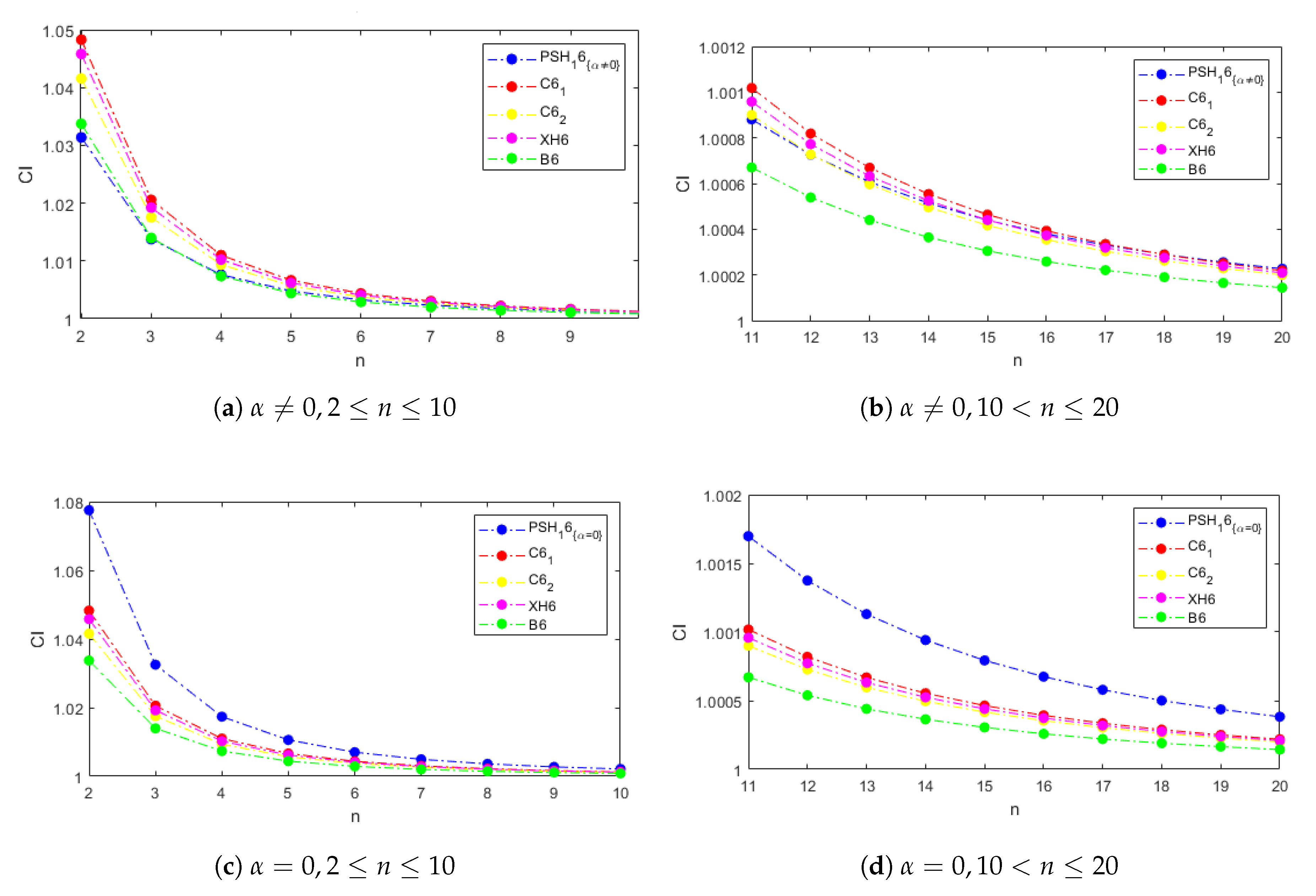
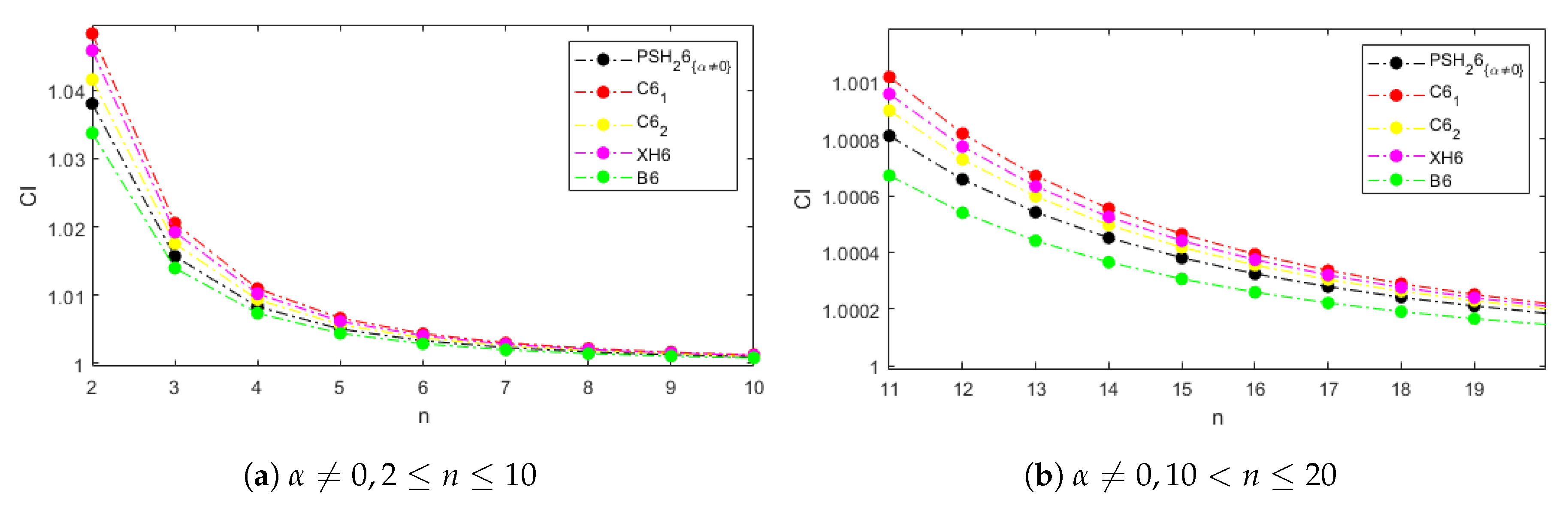
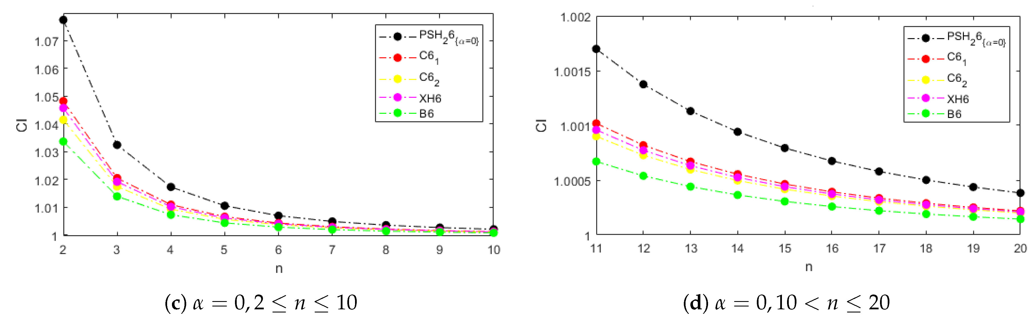
Figure 1 and Figure 2 show the computational efficiency index for the examined methods and systems of size from 2 to 20 with weight functions $H_1$ and $H_2$, respectively, in the cases of the proposed schemes. In Figure 1a,b, the parameter $\alpha$ is not null, and in Figure 1c,d it is equal to zero. Let us notice that the behavior of the $CI$ for the weight functions $H_1$ and $H_2$ is the same when $\alpha =0$ and it is better than those of the comparison methods. This performance is explained for the dominating term $\frac{1}{3}{n}^3$ in the computational cost calculation; it is due to the existence of only one type of linear systems to be solved per iteration with the matrix of coefficients $F^{\prime }(x)$.

Let us also remark that, even when $\alpha \ne 0$, our methods are competitive with the existing ones, especially in systems with size higher than 10, where the differences among the indices of all the methods are not significant (see Figure 1b and Figure 2b).

4. Numerical Results

In this section, we compare the numerical performance of the proposed methods PSH6${}_1$ described in Expression (14) with $\alpha =0$, $\alpha =5.5$ and $\alpha =10$, PSH6${}_2$ (see Equation (16)) for the same values of the parameter $\alpha$ and existing schemes C6${}_1$, described in Equation (1); C6${}_2$ is expressed in Equation (2), XH6 appears in Equation (3) and the B6 scheme is expressed in Equation (4), with $b_1=3$.

To get this aim we use the Matlab computer algebra system, with 2000 digits of mantissa in variable precision arithmetics, to make the comparative numerical experiments. Moreover, the stopping criterion used is $\parallel x^{(k+1)}-x^{(k)}\parallel <{10}^{-200}$ or $\parallel F(x^{(k+1)})\parallel <{10}^{-200}$. The initial values employed and the searched solutions are symbolized as $x^{(0)}$ and $\xi$, respectively. When the iterative expression of the method involves the evaluation of a divided difference operator, it is calculated by using the first-order estimation of the Jacobian matrix whose elements are (see [27])

$${[a,b;F]}_{ij}=\frac{F_i(a_1,...,a_{j-1},a_j,b_{j+1},...,b_m)-F_i(a_1,...,a_{j-1},b_j,b_{j+1},...,b_m)}{a_j-b_j},1\le i,j\le n.$$

where $F_i$ and $i=1,2,\dots ,n$ are the coordinate functions of F.

For each nonlinear function, one table will be displayed with the results of the numerical experiments. The given information is organized as follows: k is the number of iteration needed to converge to the solution (’nc’ appears in the table if the method does not converge), the value of the stopping residuals is $\parallel x^{(k+1)}-x^{(k)}\parallel$ or $\parallel F(x^{(k+1)})\parallel$ at the last step (’-’ if there is no convergence) and the approximated computational order of convergence is $\rho$ (if the value of $\rho$ for the last iterations is not stable, then ’-’ appears in the table). In this way, it can be checked if the convergence has reached the root ($\parallel F(x^{(k+1)})\parallel <{10}^{-200}$ is achieved), if it is only a very slow convergence with no significant difference between the two last iterations ($\parallel x^{(k+1)}-x^{(k)}\parallel <{10}^{-200}$ but $\parallel F(x^{(k+1)})\parallel >{10}^{-200}$), or both criteria are satisfied.

The test systems used are defined by the following nonlinear functions:

Example 1.

The first nonlinear system, whose solution is $\xi ={(0.0,0.0)}^T$, is described by function

$$F_1(x_1,x_2)=(sin(x_1)+x_{2}sin(x_1),x_1-x_2).$$

Our test is made by using as initial estimation $x^{(0)}={(0.8,0.8)}^T$ and the results appear in

Table 3. Numerical results of the examined methods for $F_1(x_1,x_2)$ and $x^{(0)}={(0.8,0.8)}^T$.

Method	k	$\parallel {\mathit{x}}^{(\mathit{k}+1)}-{\mathit{x}}^{(\mathit{k})}\parallel$	$\parallel \mathit{F}({\mathit{x}}^{(\mathit{k}+1)})\parallel$	$\mathit{\rho }$
$\mathrm{PSH}{6}_1\{\alpha =0.0\}$	4	$5.7517\times {10}^{-60}$	0.0	5.9906
$\mathrm{PSH}{6}_1\{\alpha =5.5\}$	4	$2.0238\times {10}^{-64}$	0.0	5.9962
$\mathrm{PSH}{6}_1\{\alpha =10\}$	4	$2.9651\times {10}^{-78}$	0.0	6.0264
$\mathrm{PSH}{6}_2\{\alpha =0.0\}$	4	$5.7517\times {10}^{-60}$	0.0	5.9906
$\mathrm{PSH}{6}_2\{\alpha =5.5\}$	4	$1.0081\times {10}^{-46}$	$3.6422\times {10}^{-275}$	5.9701
$\mathrm{PSH}{6}_2\{\alpha =10\}$	4	$6.6149\times {10}^{-43}$	$6.8963\times {10}^{-252}$	5.9523
$\mathrm{C}{6}_1$	4	$1.5912\times {10}^{-73}$	0.0	5.9973
$\mathrm{C}{6}_2$	10	$6.3065\times {10}^{-72}$	0.0	5.9975
$\mathrm{XH}6$	4	$8.6943\times {10}^{-66}$	0.0	5.9953
$\mathrm{B}6$	4	$5.0674\times {10}^{-80}$	0.0	6.0030

.

In Table 3, it can be observed that, except for method C6${}_2$, all the compared schemes converge to the solution in four iterations, with null (for the fixed precision of the machine at 2000 digits) or almost null residual $\parallel F(x^{(k+1)})\parallel$. Moreover, the computational approximation order of convergence agrees in all cases with the theoretical one.

Example 2.

The following nonlinear function describes a system with solution $\xi \approx {(2.4914,0.2427,1.6535)}^T$,

$$F_3(x_1,x_2,x_3)=(x_1^2+x_2^2+x_3^2-9,x_1{x}_2{x}_3-1,x_1+x_2-x_3^2).$$

We test all the new and existing methods with this system with the initial estimation $x^{(0)}={(2.0,0.5,1.0)}^T$ and the results are provided in

Table 4. Numerical results of the examined methods for $F_3(x_1,x_2,x_3)$ and $x^{(0)}={(2.0,0.5,1.0)}^T$.

Method	k	$\parallel {\mathit{x}}^{(\mathit{k}+1)}-{\mathit{x}}^{(\mathit{k})}\parallel$	$\parallel \mathit{F}({\mathit{x}}^{(\mathit{k}+1)})\parallel$	$\mathit{\rho }$
$\mathrm{PSH}{6}_1\{\alpha =0.0\}$	5	$1.1553\times {10}^{-91}$	0.0	-
$\mathrm{PSH}{6}_1\{\alpha =5.5\}$	5	$1.3862\times {10}^{-138}$	0.0	-
$\mathrm{PSH}{6}_1\{\alpha =10\}$	5	$3.1738\times {10}^{-101}$	$0.0$	-
$\mathrm{PSH}{6}_2\{\alpha =0.0\}$	5	$1.1553\times {10}^{-91}$	0.0	-
$\mathrm{PSH}{6}_2\{\alpha =5.5\}$	6	$6.4700\times {10}^{-85}$	0.0	-
$\mathrm{PSH}{6}_2\{\alpha =10\}$	6	$2.7383\times {10}^{-132}$	$0.0$	-
$\mathrm{C}{6}_1$	4	$5.5171\times {10}^{-38}$	$7.1730\times {10}^{-225}$	6.0424
$\mathrm{C}{6}_2$	4	$2.1522\times {10}^{-93}$	0.0	6.0006
$\mathrm{XH}6$	4	$6.1878\times {10}^{-50}$	$5.5325\times {10}^{-297}$	5.9482
$\mathrm{B}6$	4	$5.1979\times {10}^{-168}$	0.0	6.0365

.

In this example, the proposed methods take at least one more iteration to converge to the solution (see Table 4). However, the precision of the results are the same or even better than those of the known methods, as $\parallel F(x^{(k+1)})\parallel$ is null in all new cases.

Example 3.

Now, we test the methods with the nonlinear system described by

$$F_4(x_1,x_2,x_3,x_4)=(x_1{x}_2+x_4(x_1+x_2),x_1{x}_3+x_4(x_1+x_3),x_2{x}_3+x_4(x_2+x_3),x_1{x}_2+x_1{x}_3+x_2{x}_3-1),$$

using as the initial guess $x^{(0)}={(2.5,2.5,2.5,2.5)}^T$. The searched root is $\xi \approx {(0.5774,0.5774,0.5774,-0.2887)}^T$ and we can find the residuals, the number of iterations needed to converge and the estimated order of convergence in

Table 5. Numerical results of the examined methods for $F_4(x_1,x_2,x_3,x_4)$ and $x^{(0)}={(2.5,2.5,2.5,2.5)}^T$.

Method	k	$\parallel {\mathit{x}}^{(\mathit{k}+1)}-{\mathit{x}}^{(\mathit{k})}\parallel$	$\parallel \mathit{F}({\mathit{x}}^{(\mathit{k}+1)})\parallel$	$\mathit{\rho }$
$\mathrm{PSH}{6}_1\{\alpha =0.0\}$	5	$1.7213\times {10}^{-82}$	0.0	5.8841
$\mathrm{PSH}{6}_1\{\alpha =5.5\}$	5	$6.2032\times {10}^{-101}$	0.0	6.0319
$\mathrm{PSH}{6}_1\{\alpha =10\}$	5	$5.9604\times {10}^{-139}$	$0.0$	7.0104
$\mathrm{PSH}{6}_2\{\alpha =0.0\}$	5	$1.7213\times {10}^{-82}$	0.0	5.8841
$\mathrm{PSH}{6}_2\{\alpha =5.5\}$	5	$2.4280\times {10}^{-56}$	0.0	5.4681
$\mathrm{PSH}{6}_2\{\alpha =10\}$	5	$2.2166\times {10}^{-50}$	$0.0$	5.2317
$\mathrm{C}{6}_1$	4	$2.8009\times {10}^{-167}$	0.0	6.1732
$\mathrm{C}{6}_2$	4	$6.0097\times {10}^{-36}$	$9.3590\times {10}^{-222}$	6.7740
$\mathrm{XH}6$	5	$1.0184\times {10}^{-173}$	0.0	6.1665
$\mathrm{B}6$	4	$9.0970\times {10}^{-198}$	0.0	5.6982

.

A similar performance can be observed in Table 5 where the effective stopping criterium is that involving the evaluation of the nonlinear function and the residual is null most times. However, the number of iterations needed does not improve on the number provided for most of known methods.

Example 4.

Finally we test the proposed and existing methods with a nonlinear system of variable size. It is described as

$${\displaystyle x_i-\cos \left(2x_i-\sum _{j=1}^4{x}_j\right)=0,i=1,2,\dots ,n,}$$

with $n=20$ and starting with the estimation $x^{(0)}={(0.75,\dots ,0.75)}^T$. In this case, the solution is $\xi \approx {(0.5149,\dots ,0.5149)}^T$ and the obtained results can be found at

Table 6. Numerical results of proposed methods for $F_5(x_1,x_2,\dots ,x_n)$, $n=20$ and $x^{(0)}={(0.75,\dots ,0.75)}^T$.

Method	k	$\parallel {\mathit{x}}^{(\mathit{k}+1)}-{\mathit{x}}^{(\mathit{k})}\parallel$	$\parallel \mathit{F}({\mathit{x}}^{(\mathit{k}+1)})\parallel$	$\mathit{\rho }$
$\mathrm{PSH}{6}_1\{\alpha =0.0\}$	4	$1.8871\times {10}^{-184}$	0.0	6.0
$\mathrm{PSH}{6}_1\{\alpha =5.5\}$	4	$1.1531\times {10}^{-189}$	0.0	6.0
$\mathrm{PSH}{6}_1\{\alpha =10\}$	4	$2.8662\times {10}^{-195}$	0.0	6.0
$\mathrm{PSH}{6}_2\{\alpha =0.0\}$	4	$1.8871\times {10}^{-184}$	0.0	6.0
$\mathrm{PSH}{6}_2\{\alpha =5.5\}$	4	$2.0650\times {10}^{-171}$	0.0	6.0
$\mathrm{PSH}{6}_2\{\alpha =10\}$	4	$4.6908\times {10}^{-165}$	0.0	6.0
$\mathrm{C}{6}_1$	3	$9.2604\times {10}^{-39}$	$7.5226\times {10}^{-233}$	5.7540
$\mathrm{C}{6}_2$	4	$9.7326\times {10}^{-195}$	0.0	6.0
$\mathrm{XH}6$	4	$2.4997\times {10}^{-191}$	0.0	6.0
$\mathrm{B}6$	6	$5.7210\times {10}^{-197}$	0.0	6.0

.

When the systems are large, as in the case of $F_5(x_1,x_2,\dots ,x_n)$, where $n=20$, our schemes provide excellent results, equalling or improving the performance of existing procedures, see Table 6. The number of iterations needed to satisfy one of the stopping criteria and the residuals obtained show a very competitive performance. Moreover, the theoretical order of convergence is estimated with full precision.

5. Conclusions

In this work, we have proposed an efficient class of iterative schemes, with two specific subfamilies with very good performance. We have also compared them with other existing methods of the same order, with good results. The choice of parameters for the different proposed subfamilies does not pursue a specific objective but the dependence of the convergence on the selection of parameter $\alpha$ is considered for further studies. Being similar, the numerical experiments show slightly better behavior for PS6$H_1$ than for PS6$H_2$, in comparison with the existing procedures.

References

- Traub, J.F. Iterative Methods for the Solution of Equations; Prentice Hall: New York, NY, USA, 1964. [Google Scholar]
- Cordero, A.; Torregrosa, J.R.; Vassileva, M.P. Design, Analysis, and Applications of Iterative Methods for Solving Nonlinear Systems. In Nonlinear Systems—Design, Analysis, Estimation and Control; InTech: London, UK, 2016. [Google Scholar] [CrossRef]
- Amat, S.; Busquier, S. Advances in Iterative Methods for Nonlinear Equations; SEMA SIMAI Springer Series: New York, NY, USA, 2016. [Google Scholar]
- Cordero, A.; Torregrosa, J.R.; Vassileva, M.P. Pseudo-composition: A technique to design predictor-corrector methods for systems of nonlinear equations. Appl. Math. Comput. 2012, 218, 11496–11508. [Google Scholar]
- Babolian, E.; Biazar, J.; Vahidi, A.R. Solution of a system of nonlinear equations by Adomian decomposition method. Appl. Math. Comput. 2004, 150, 847–854. [Google Scholar] [CrossRef]
- Darvishi, M.T.; Barati, A. Super cubic itertive methods to solve systems of nonlinear equations. Appl. Math. Comput. 2007, 188, 1678–1685. [Google Scholar]
- Cordero, A.; Martínez, E.; Torregrosa, J.R. Iterative methods of order four and five for systems of nonlinear equations. J. Comput. Appl. Math. 2009, 231, 541–551. [Google Scholar] [CrossRef] [Green Version]
- Hernández, M.A. Second-derivative-free variant of the Chebyshev method for nonlinear equations. J. Opt. Theory Appl. 2000, 104, 501–515. [Google Scholar] [CrossRef]
- Hueso, J.L.; Martínez, E.; Torregrosa, J.R. Third and fourth order iterative methods free from second derivative for nonlinear systems. Appl. Math. Comput. 2009, 211, 190–197. [Google Scholar] [CrossRef]
- Soleymani, F.; Sharifi, M.; Shateyi, S.; Haghani, F.K. A class of Steffensen-type iterative methods for nonlinear systems. J. Appl. Math. 2014, 2014, 705375. [Google Scholar] [CrossRef]
- Singh, A. An efficient fifth-order Steffensen-type method for solving systems of nonlinear equations. Int. J. Comput. Sci. Math. 2018, 9, 501–514. [Google Scholar] [CrossRef]
- Sharma, J.R.; Arora, H. Efficient derivative-free numerical methods for solving systems of nonlinear equations. Comput. Appl. Math. 2016, 35, 269–284. [Google Scholar] [CrossRef]
- Cordero, A.; Jordán, C.; Sanabria, E.; Torregrosa, J.R. A new Class of iterative Processes for Solving Nonlinear Systems by using One Divided Differences Operator. Mathematics 2019, 7, 776. [Google Scholar] [CrossRef] [Green Version]
- Narang, M.; Bhatia, S.; Alshomrani, A.S.; Kanwar, V. General efficient class of Steffensen type methods with memory for solving systems of nonlinear equations. J. Comput. Appl. Math. 2019, 352, 23–39. [Google Scholar] [CrossRef]
- Candela, V.; Peris, R. A class of third order iterative Kurchatov–Steffensen (derivative free) methods for solving nonlinear equations. Appl. Math. Comput. 2019, 350, 93–104. [Google Scholar] [CrossRef]
- Cordero, A.; Maimó, J.G.; Torregrosa, J.R.; Vassileva, M.P. Iterative Methods with Memory for Solving Systems of Nonlinear Equations Using a Second Order Approximation. Mathematics 2019, 7, 1069. [Google Scholar] [CrossRef] [Green Version]
- Li, J.; Huang, P.; Su, J.; Chen, Z. A linear, stabilized, nonspatial iterative, partitioned time stepping method for the nonlinear Navier-Stokes/Navier-Stokes interaction model. Bound. Value Probl. 2019, 2019, 115. [Google Scholar] [CrossRef] [Green Version]
- Sharma, J.R.; Guha, R.K.; Sharma, R. An efficient fourth-order weighted-Newton method for systems of nonlinear equations. Numer. Algorithms 2013, 62, 307–323. [Google Scholar] [CrossRef]
- Artidiello, S.; Cordero, A.; Torregrosa, J.R.; Vassileva, M.P. Multidimensional generalization of iterative methods for solving nonlinear problems by means of weight-function procedure. Appl. Math. Comput. 2015, 268, 1064–1071. [Google Scholar] [CrossRef] [Green Version]
- Artidiello, S.; Cordero, A.; Torregrosa, J.R.; Vassileva, M.P. Design and multidimensional extension of iterative methods for solving nonlinear problems. Appl. Math. Comput. 2017, 293, 194–203. [Google Scholar] [CrossRef]
- Abad, M.; Cordero, A.; Torregrosa, J.R. A family of seventh-order schemes for solving nonlinear systems. Bulletin Mathématique (Societe des Sciences Mathematiques de Roumanie) 2014, 57, 133–145. [Google Scholar]
- Cordero, A.; García-Maimó, J.; Torregrosa, J.R.; Vassileva, M.P. Solving nonlinear problems by Ostrowski-Chun type parametric families. J. Math. Chem. 2015, 53, 430–449. [Google Scholar] [CrossRef] [Green Version]
- Cordero, A.; Hueso, J.L.; Martínez, E.; Torregrosa, J.R. Increasing the convergence order of an iterative method for nonlinear systems. Appl. Math. Lett. 2012, 25, 2369–2374. [Google Scholar] [CrossRef] [Green Version]
- Cordero, A.; Hueso, J.L.; Martínez, E.; Torregrosa, J.R. A modified Newton-Jarrat composition. Numer. Algorithms 2010, 55, 87–99. [Google Scholar] [CrossRef]
- Xiao, X.Y.; Yin, H.W. Increasing the order of convergence for iterative methods to solve nonlinear systems. Calcolo 2016, 53, 285–300. [Google Scholar] [CrossRef]
- Behl, R.; Sarría, Í.; González, R.; Magreñán, Á.A. Highly efficient family of iterative methods for solving nonlinear models. J. Comput. Appl. Math. 2019, 346, 110–132. [Google Scholar] [CrossRef]
- Ortega, J.M.; Rheinbolt, W.C. Iterative Solutions of Nonlinears Equations in Several Variables; Academic Press: New York, NY, USA, 1970. [Google Scholar]
- Ostrowski, A.M. Solution of Equations and System of Equations; Prentice Hall: Englewood Cliffs, NJ, USA, 1964. [Google Scholar]
- Cordero, A.; Torregrosa, J.R. On interpolation variants of Newton’s method for functions of several variables. J. Comput. Appl. Math. 2010, 234, 34–43. [Google Scholar] [CrossRef] [Green Version]
Figure 1.
indices for PSH6 and comparison methods.
Figure 2.