Graphs Based on Hoop Algebras


1
Hatef Higher Education Institute, Zahedan 8301, Iran
2
Department of Mathematics, Shahid Beheshti University, Tehran 7561, Iran
3
Research Institute for Natural Science, Department of Mathematics, Hanyang University, Seoul 04763, Korea
*
Author to whom correspondence should be addressed.
Mathematics 2019, 7(4), 362; https://0-doi-org.brum.beds.ac.uk/10.3390/math7040362
Submission received: 14 March 2019
/
Revised: 13 April 2019
/
Accepted: 17 April 2019
/
Published: 21 April 2019
(This article belongs to the Special Issue General Algebraic Structures)
Abstract
:In this paper, we investigate the graph structures on hoop algebras. First, by using the quasi-filters and r-prime (one-prime) filters, we construct an implicative graph and show that it is connected and under which conditions it is a star or tree. By using zero divisor elements, we construct a productive graph and prove that it is connected and both complete and a tree under some conditions.
MSC:
06F99; 03G25; 18B35; 22A261. Introduction
Non-classical logic has become a formal and useful tool for computer science to deal with uncertain information and fuzzy information. The algebraic counterparts of some non-classical logics satisfy residuation and those logics can be considered in a frame of residuated lattices [1]. For example, Hájek’s BL (basic logixc [2]), Lukasiewicz’s MV (many-valued logic [3]) and MTL (monoidal t-norm-based logic [4]) are determined by the class of BL-algebras, MV-algebras and MTL-algebras, respectively. All of these algebras have lattices with residuation as a common support set. Thus, it is very important to investigate properties of algebras with residuation.
Hoops are naturally ordered commutative residuated integral monoids, as introduced by Bosbach [5,6], and then studied by Büchi and Owens, in a paper never published. In the last years, hoop theory has been enriched with deep structure theorems [7,8,9,10]. Many of these results have a strong impact with fuzzy logic.
Graph theory has existed for many years not only as an area of mathematical study, but also as an intuitive and illustrative tool. Graph theory has found many applications in engineering and science, such as chemical, electrical, civil and mechanical engineering; architecture; management and control; communication; operational research; sparse matrix technology; combinatorial optimization; and computer science. Therefore, many books have been published on applied graph theory, e.g. the book by Bondy and Murty [11]; especially in the field of universal algebras and graph theory, graph algebra is a way of giving a directed graph of algebraic structure. This was introduced by McNulty [12], and has seen many uses in the field of universal algebra since then. Algebraic graph theory comprises both the study of algebraic objects arising in connection with graphs. The rapidly expanding area of algebraic graph theory uses two different branches of algebra to explore various aspects of graph theory: linear algebra (for spectral theory) and group theory (for studying graph symmetry). These areas have links with other areas of mathematics, such as logic and harmonic analysis, and are increasingly being used in such areas as computer networks where symmetry is an important feature, for example, automorphism groups of graphs along with the use of algebraic tools to establish interesting properties of combinatorial objects. One of the oldest themes in the area is the investigation of the relation between properties of a graph and the spectrum of its adjacency matrix. In addition, algebraic graph theory can be viewed as an extension to graph theory in which algebraic methods are applied to problems about graphs. Many authors studied graph theory in connection with semigroups and rings. In [13], Beck introduced the zero-divisor graph associated with the zero-divisor set of a commutative ring, whose vertex set is the set of zero divisors. Two distinct zero divisors are adjacent in if and only if . The zero-divisor graph establishes a connection between graph theory and commutative ring theory, which hopefully will turn out to be mutually beneficial for those two branches of mathematics. Axtell and Stickles [14], remarked that, in general, the set of zero-divisors lacks algebraic structure, suggesting that turning to the zero-divisor graph may both reveal both ring-theoretical properties and impose a graph-theoretical structure. Beck’s hopes have certainly been met: his now classical paper motivated an explosion of research in this and similar associated graphs in the past decade. His definition has since been modified to emphasize the fundamental structure of the zero-divisor set: Anderson’s definition given in [15], which excludes the vertex 0 from the graph, is now considered standard. In [16], Jun and Lee introduced the notion of associated graph of BCK/BCI-algebras by zero divisors in BCK/BCI-algebras and verified some properties of this graph. In addition, Torkzadeh and Ahmadpanah [17] defined the notion of zero divisors of a non-empty subset A of a residuated lattice L and associated a graph to a residuated lattice L. They proved that this graph is always a connected graph and its diameter is at most two.
In this paper, the graphs of hoop algebras are studied. For this, the notion of zero divisors of a non-empty subset of a hoop algebra is introduced by two methods and some related properties are investigated. Several examples of hoop graphs are proved. These graphs are connected and also some necessary conditions for the hoop graph to be a star graph are found. Finally, hoop graphs that are provided by two methods together are compered.
2. Preliminaries
At first, we recall the definition of a hoop algebra and some properties.
By a hoop, we mean an algebraic structure where, for all :
- (HP1)
- is a commutative monoid.
- (HP2)
- .
- (HP3)
- .
- (HP4)
- .
On hoop A we define if and only if . It is easy to see that ≤ is a partial order relation on A. A hoop A is bounded if there is an element such that , for all .
Let A be a bounded hoop. We define a negation “−” on A by , for all . For , we define . If , for all , then the bounded hoop A is said to have the double negation property (DNP).
The following proposition provides some properties of hoops.
Proposition 1
- (i)
- is a meet-semilattice with .
- (ii)
- if and only if .
- (iii)
- and .
- (iv)
- and .
- (v)
- .
- (vi)
- .
- (vii)
- and .
- (viii)
- implies and and .
Let A be a hoop and for any ; define
Then, a hoop A is called a ⊔-hoop, if ⊔ is the join operation on A. It is easy to see that, for any ,
A non-empty subset I of ⊔-hoop A is called an ideal of A if it satisfies the following conditions:
- (I1)
- If , then .
- (I2)
- If , and , then .
A non-empty subset F of A is a filter of A if,
- (F1)
- implies .
- (F2)
- and imply , for any .
The set of all filters of A is denoted by . F is a proper filter if F is a filter of A and . A proper filter of A is called a maximal filter, if it is not properly contained in any other proper filters of A.
Let G be a graph with the vertex set V and edge set E. The edge that connects two distinct vertices x and y is denoted by . Note that and are the same. A graph is called a subgraph of , if and . A graph is called connected, if any two distinct vertices x and y of G linked by a path in G, otherwise the graph is called disconnected. For distinct vertices x and y of G, let be the length of the shortest path from x to y. If there is no path, then . The diameter of G is
A tree is a connected graph with no cycles. A graph G is called complete graph if , for any distinct elements . A graph G is called a star graph in the case there is a vertex x in G such that every other vertex in G is an end, connected to x and no other vertex by an edge [18].
Notation. From now on, or simply A is a hoop algebra, unless otherwise stated.
3. Implicative Graph of a Hoop Algebra
In this section, we study associated implicative graph of a hoop algebra. We first introduce the notions of r-prime quasi-filter and zero divisors and investigate related properties. Then, we introduce the concept of associated implicative graph of a hoop A and provide several examples.
Notation. For any non-empty subset X of A, we use the notation and to denote the sets,
Definition 1.
Let F be a non-empty subset of A. Then,
- (i)
- F is called a quasi-filter of A if for all , and , then .
- (ii)
- A quasi-filter F of A is called a r-prime (l-prime) filter if it satisfies the following conditions:F is proper, that is ; andfor any , if , then or .
Example 1.
Let . Define the operations ⊙ and → on A as follows
We can easily see that A with these operations is a bounded hoop. Let and . Then, by routine calculation, we can see that and . Now, and are quasi-filters of A but G is not a filter of A, because . Moreover, F is an r-prime filter of A.
Proposition 2.
Let X and Y be two non-empty subsets of A. Then, the following statements hold:
- (i)
- and .
- (ii)
- If , then and .
- (iii)
- and .
Proof.
Let . Then, for any and for any , we get that . Thus, we have for any and for any , . Hence, . Therefore, . Similarly, we can prove that .
Let . Then, for any , . Since , for any , , too. Hence, . Similarly, .
By (i), , then by (ii), . Let . Then, by (i), , and thus . Hence, . Similarly, . □
Theorem 1.
A proper quasi-filter F of A is r-prime if and only if implies, there exists such that .
Proof.
We proceed by induction on n. If , then . Since F is an r-prime quasi-filter of A, by Definition 1, the result is clear. Now, suppose the statement holds for . Let such that . If , then by routine calculation, we can see that
Now, assume that . Since F is r-prime, we get , which shows that . Using the induction hypothesis, we conclude that , for some . The converse is clear. □
Remark 1.
- (i)
- For any , . Thus, .
- (ii)
- , for any . Thus, we have,
Definition 2.
For any , we use the notion to denote the set of all elements such that . It means that .
Example 2.
According to Example 1,
Proposition 3.
For any , .
Proof.
Let . Since
we have . □
Proposition 4.
For any elements a and b of A, if , then and .
Proof.
Let . Then, . By assumption, , then by Proposition 1(vi), . Then, , and thus . Thus, . Hence, . Now, suppose . Then, by Remark 1(ii),
Thus, , and so . Therefore, . □
By the following example, we show that the converse of relation in Proposition 4 may not be true in general.
Example 3.
In Example 1, . By routine calculation, we have , , and . We can easily see that and .
Theorem 2.
For any element x of A, is a quasi-filter of A containing the element 1. Moreover, if is maximal in , then is an r-prime.
Proof.
At first, we prove that is a quasi-filter of A. For this, suppose and are two arbitrary elements such that . Then, it is enough to prove that . Since , we have . By Proposition 4, . In addition, since , we have . Moreover, we know that , then by Remark 1,
Thus, . Hence, . Thus, is a quasi-filter of A. Now, suppose is maximal in . By Proposition 3, for any , . Then, , and so . Now, we prove that is an r-prime. For this, let and such that . It is enough to prove that . Since is maximal, is proper. Moreover, since such that , . Suppose . Then,
Let . Then, there exists such that . Since , we have . In addition, , then . Moreover, since and , we have , which is a contradiction. Then, , and thus . In addition, from , . Then, there exists , and so . Thus, by Proposition 4, . If , then, for any , , and so . Since , we get . In addition, , then , which is a contradiction. Then, is proper. Since is maximal, . In addition, from , we have,
Then, , thus . Since , we get . Thus, is an r-prime of A. □
Definition 3.
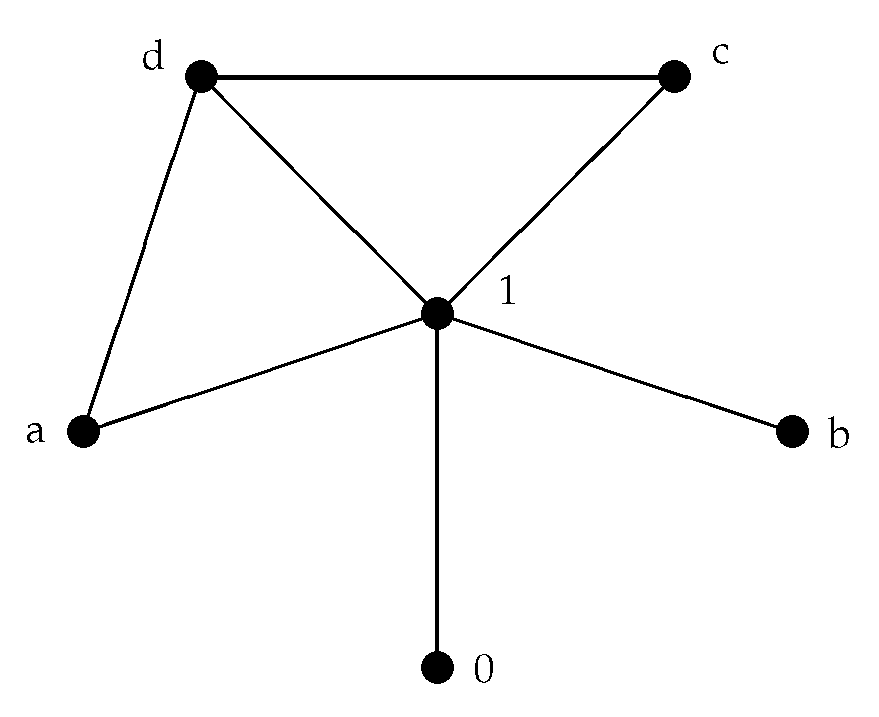
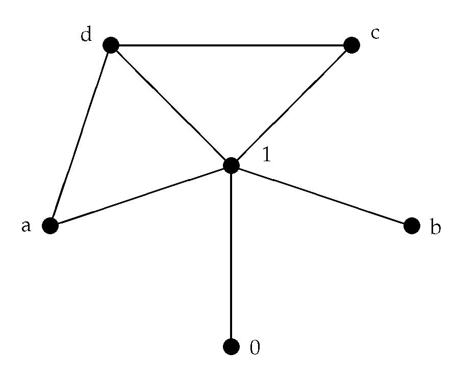
By the implicative graph of a hoop A, denoted , we mean the graph which vertices are just the elements of A, and for distinct , there is an edge connecting x and y if and only if .
Example 4.
According to Example 1, we have, and , as Figure 1.
Theorem 3.
For any , if and are distinct r-prime quasi-filters of A, then there is an edge connecting x and y.
Proof.
Let . It is sufficient to prove that . Suppose . Then, and . If , then , which is a contradiction. Let . Then, . Since is a quasi-filter, , thus, . By assumption, is an r-prime, then or . Since , we get that . Hence, . Similarly, we can see that . Thus, , which is a contradiction. By assumption, and are distinct. Therefore, and there is an edge connecting x and y. □
Theorem 4.
The graph is connected with diameter at most two.
Proof.
By Proposition 3, for any , . Then, 1 is connected to all points of A. Hence, both vertices are connected by a path, and so is connected. Now, let be two vertices in . If , then . If , then the path exists, thus, . Since
we have . □
Theorem 5.
If A is a totally ordered hoop, then is a star.
Proof.
Suppose A is a totally ordered hoop and . We proceed by induction on n. If , then . Since , it is enough to investigate on . It is easily to see that . Then, 1 is just connected to all points of A, and so is a star. Let . Without loss of generality, suppose such that . Using the induction hypothesis, we conclude that is a star such that and . Suppose . By assumption, for any , , then it is easy to see that
Thus, there is no edge . Hence, is a star. □
Corollary 1.
If A is a totally ordered hoop, then is a tree.
4. Productive Graph of a Hoop Algebra
In this section, we study associated productive graph of a hoop algebra. We first introduce the notion of zero divisors by product operation and investigate related properties. By means of the set of all zero divisors of elements of a hoop A, the associated productive graph is defined and several examples are provided.
Note. From now one, in this section, A will be a bounded hoop algebra.
Definition 4.
Let X be a non-empty subset of A. The set of all zero divisors of X is denoted by and is defined as follows:
Proposition 5.
Let X and Y be non-empty subsets of A. Then, the following statements hold:
- (i)
- .
- (ii)
- If , then .
- (iii)
- If , then .
- (iv)
- If , then .
- (v)
- , for all .
- (vi)
- if and only if if and only if .
- (vii)
- If , then .
- (viii)
- , where .
Proof.
Since A is a bounded hoop, then . Thus, for any , . Hence, .
Let . Then, for any , . Since , for any , . Hence, . Therefore, .
Assume that , then , for all . Put , for . Hence, , for all , and we get that , for all . Since , then , for all , i.e, , for all . Thus, we can obtain , that is , for all . Therefore, .
Let and . Then, , and so .
The proof follows by (iv).
Let . Then, , for all and so . Conversely, let . Then, . We get that . It is easy to prove that if and only if .
The proof is straightforward.
Let . Then, by Definition 4, or , for all or . Suppose , for all . Since , by Proposition 1(viii), . From , we have . Hence, . □
By the following example, we show that the inverse inclusions of Proposition 5(iii) and (viii) may not be true, in general.
Example 5.
According to Example 1:
Let . Then, by routine calculations, we can see that , Thus, , and so . Hence, . Thus, it is clear that .
Let and . Then, and , respectively. Thus, . We can easily see that and . Hence, .
Proposition 6.
Let X be a non-empty subset of ⊔-hoop A. Then, is an ideal of A.
Proof.
By Proposition 5(i), , then is non-empty. Let , for any and . Then, , for all . By Proposition 1(viii), , then , for all . Thus, . Now, let . Then, , for all . Hence, for all ,
that is . Therefore, is an ideal of A. □
For , the set is called the set of all zero divisors of x.
By Proposition 5, we have and , for all .
Proposition 7.
is a filter of A, for any .
Proof.
Let . Then, by Proposition 5(iv), , thus, , i.e., . Now, we show that is a filter of A. Let . Then, . Suppose . Then, . Since A is a monoid, , then . Hence, . Since , we have . Thus, , and so . Now, suppose and such that . Let . Then, . Since , by Proposition 1(viii), , then . Thus, . Hence, . Then, , and so . Therefore, . □
The set of dense elements of a hoop A is denoted by .
Theorem 6.
.
Proof.
Let . Then,
Since and by Proposition 1(vii), , we have . Then, , and so . Conversely, let . Then, . Since and by Proposition 1(vii), , . Now, suppose . Then, , and so . Since , we have . Thus, . Hence, . □
Definition 5.
is called an associated productive graph if vertices are just the elements of A, and for distinct , there is an edge connecting x and y if and only if . The edge that connects two vertices x and y is denoted by .
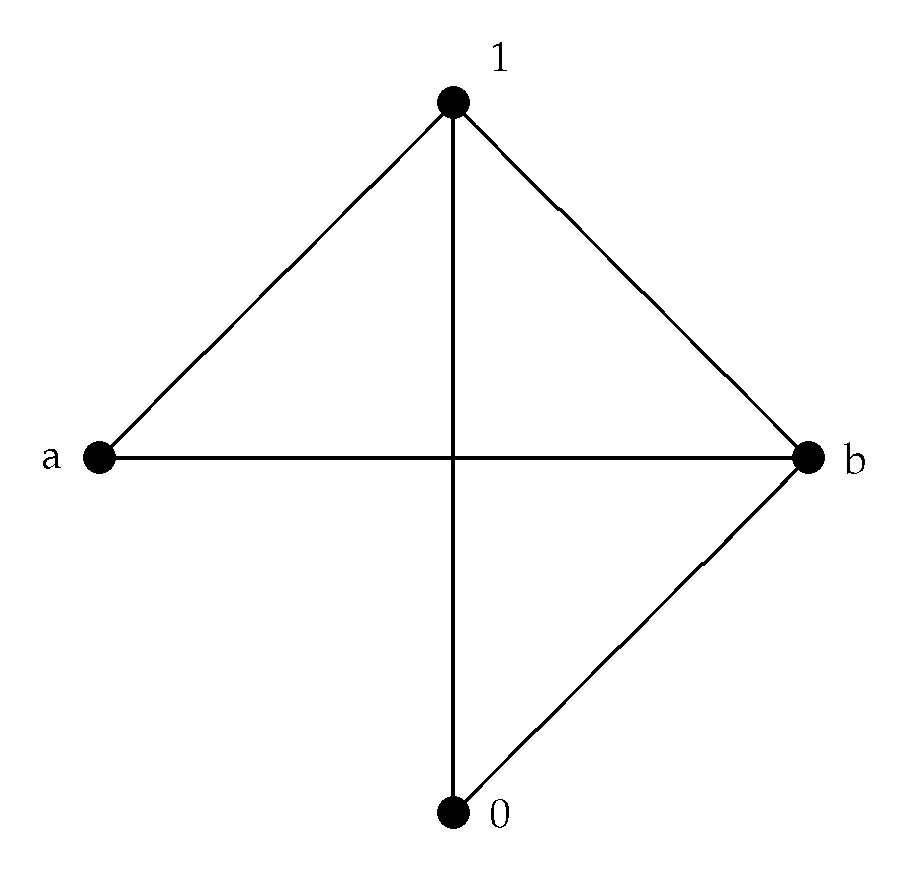
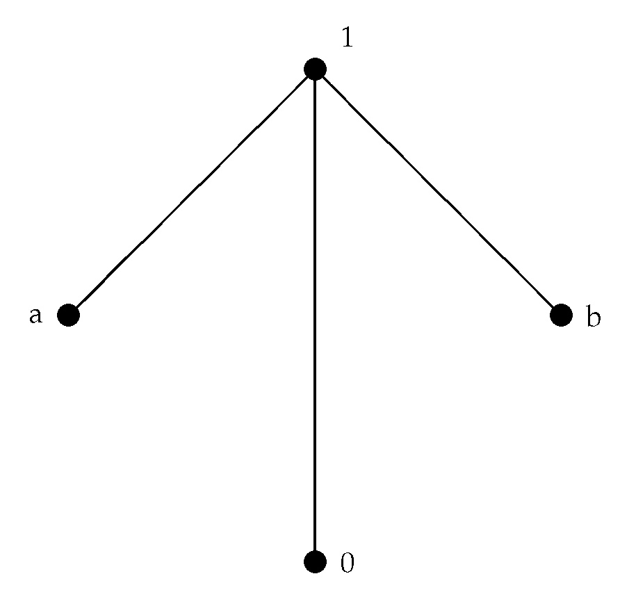
Example 6.
Let . Define the operations ⊙ and → on A as follows
By routine calculations, we see that A with these operations is a bounded hoop. Then, for any , we have:
as Figure 2.
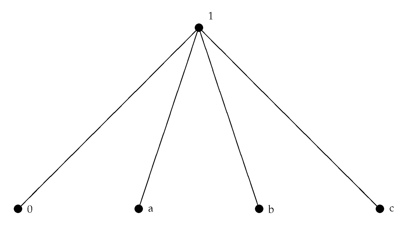
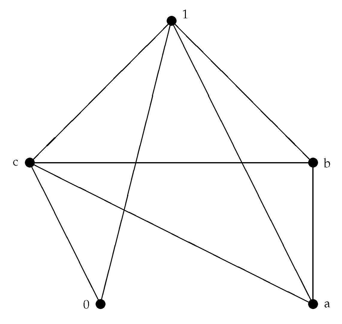
Let . Define the operations ⊙ and → on A as follows
Then, A with these operations is a bounded hoop. Then, for any , we have: , as Figure 3.
Theorem 7.
is a connected graph with diameter at most two.
Proof.
By Proposition 5(iv), , for any . Then, 1 is connected to all points of A. Hence, both vertices are connected by a path, and so is connected. Now, let be two vertices in . If , then . If , then the path exists, thus . Since
we have . □
Theorem 8.
if and only if is complete.
Proof.
Let such that . Then, , and so . By definition of ,
Since , we have . Then, . Hence, exists. By Theorem 6, , then . Thus, for any , . Hence, . Therefore, is complete.
Since is complete, for any , exists. Let and . Then, exists, and so . By Proposition 1(vii), . Then, . Thus, . Hence, . By Theorem 6, . Therefore, . □
Corollary 2.
If and , then is not a tree.
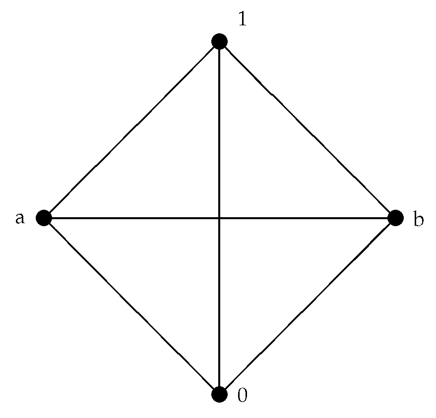
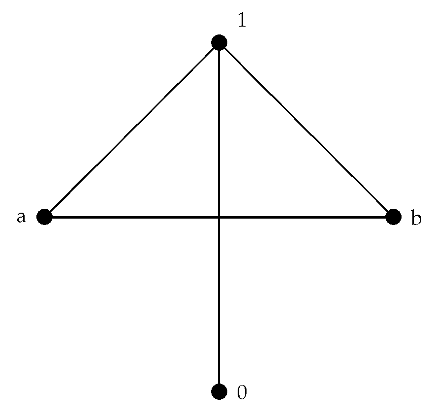
Example 7.
Let . Define the operations ⊙ and → on A as follows,
By routine calculations, we see that A with these operations is a bounded hoop and . Then, is complete. Because as Figure 4.
Theorem 9.
If is a tree, then .
Proof.
By Proposition 5(iv), , for any . Then, is connected. Since , . Suppose . Then, there exists such that . Then,
Since , . Then, the path is a circle, which is a contradiction. Because is tree. Therefore, . □
The converse of the above theorem may not be true, in general.
Example 8.
Theorem 10.
is a star graph if it satisfies the following conditions:
- (i)
- .
- (ii)
- There is such that , for any .
Proof.
By Proposition 5(iv), , for any . Then, is connected and by Theorem 7, diameter at most two. Let such that . If and or vice versa, since , we have , which is a contradiction. In addition, if , then , and so , which is a contradiction. Thus, . Thus, . Then, by (ii), there is such that . Thus, and . Hence, , and so . Then, there is not the edge . Therefore, is a star graph. □
Corollary 3.
Under Conditions (i) and (ii) of Theorem 10, is a tree.
Example 9.
Let . Define the operations ⊙ and → on A as follows
We can easily see that A with these operations is a bounded hoop. By routine calculation, we can see that two conditions of the above theorem hold because A is a chain and there is an element such that , for any . In addition, it is clear that . Thus, the graph is a star. We have: , as Figure 6.
By the following example, we show that both conditions listed in Theorem 10 are necessary.
Example 10.
Let . Define the operations ⊙ and → on A as follows
It can easily be seen that A with these operations is a bounded hoop. In this hoop neither condition holds. Because A is not a chain, there is not an element such that , for any . In addition, it is clear that , and so . We can easily see that the graph is not a star. As Figure 7, we have:
Let . Define the operations ⊙ and → on A as follows
By routine calculations, we can see that A with these operations is a bounded hoop. By routine calculation, we can see that but the second condition does not hold because A is not a chain. Thus, the graph is not a star. We have:
According to Example 7, and we see that the graph is complete. Thus, as Figure 8, it is not a star.
5. Conclusions and Future Works
In this paper, graphs of hoop algebras are studied. For this, the notion of zero divisors of a non-empty subset of a hoop algebra is introduced by two methods and some related properties are investigated. Several examples of hoop graphs are proved. These graphs are connected, and also some necessary conditions for the hoop graph to be a star graph are found. Finally, hoop graphs that are provided by two methods together are compared. Then we conclude that these graphs are connected and also some necessary conditions for the hoop graphs to be star graphs. By comparing the graph of two methods, we conclude that both graphs are connected and one is connected to all points of bounded hoop A. Finally, and are graphs with diameter at most two. However, the graph of any hoop in both methods is not the same, in general.
In our future work, we will investigate the relation between graphs and , where Π is a partition of A. In addition, we will try to find some kinds of filters in a hoop by two graphs and .
Author Contributions
The authors had the same contributions to complete the paper.
Funding
This research received no external funding.
Conflicts of Interest
The authors declare no conflicts of interest.
References
- Kowalski, T.; Ono, H. Residuated Lattices: An Algebraic Glimpse at Logic without Contraction; Japan Advanced Institute of Science and Technology: Ishikawa, Japan, 2001. [Google Scholar]
- Hájek, P. Mathematics of Fuzzy Logic; Kluwer Academic Publishers: Dordrecht, The Netherlands, 1988. [Google Scholar]
- Cingnoli, R.; Iml, D.; Mundici, D. Algebraic Foundations of Many-Valued Reasoning; Kluwer Academic Publication: Dordrecht, The Netherlands, 2000. [Google Scholar]
- Esteva, F.; Godo, L. Monoidal t-norm based logic, towards a logic for left-continuous t-norms. Fuzzy Sets Syst. 2001, 124, 271–288. [Google Scholar] [CrossRef]
- Bosbach, B. Komplementäre halbgruppen. axiomatik und arithmetik. Fundam. Math. 1969, 64, 257–287. [Google Scholar] [CrossRef]
- Bosbach, B. Komplementäre halbgruppen. Kongruenzen und Quotienten. Fundam. Math. 1970, 69, 1–14. [Google Scholar] [CrossRef]
- Borzooei, R.A.; Aaly Kologani, M. Stabilizer topology of hoops. Algebr. Struct. Their Appl. 2014, 1, 35–48. [Google Scholar]
- Borzooei, R.A.; Aaly Kologani, M. Local and perfect semihoops. J. Intell. Fuzzy Syst. 2015, 29, 223–234. [Google Scholar] [CrossRef]
- Borzooei, R.A.; Aaly Kologani, M. On Ideal Theory of Hoops. Math. Bohem. to appear.
- Namdar, A.; Borzooei, R.A.; Borumand Saeid, A.; Aaly Kologani, M. Some results in hoop algebras. J. Intell. Fuzzy Syst. 2017, 32, 1805–1813. [Google Scholar] [CrossRef]
- Bondy, J.; Murty, U.S.R.; Tutte, W.T. Graph theory and related topics. In Proceedings of the Conference Held In Honour Of Professor Wt Tutte on the Occasion of His Sixtieth Birthday, University of Waterloo, Waterloo, ON, Canada, 5–9 July 1977; Academic Press: Cambridge, MA, USA, 1979. [Google Scholar]
- McNulty, G.F.; Shallon, C.R. Caroline, Inherently nonfinitely based finite algebras. In Universal Algebra And Lattice Theory; Springer: Berlin/Heidelberg, Germany, 1983; pp. 206–231. [Google Scholar]
- Beck, I. Coloring of commutative rings. J. Algebra 1988, 116, 208–226. [Google Scholar] [CrossRef]
- Axtell, M.; Stickles, J. Graphs and zero-divisors. Coll. Math. J. 2010, 41, 396–399. [Google Scholar] [CrossRef]
- Anderson, D.; Livingston, P.S. The zero-divisor graph of a commutative ring. J. Algebra 1999, 217, 434–447. [Google Scholar] [CrossRef]
- Jun, Y.B.; Lee, K.J. Graphs based on BCK/BCI-algebras. Int. J. Math. Math. Sci. 2011, 2011, 616981. [Google Scholar] [CrossRef]
- Torkzadeh, L.; Ahmadpanah, A. Graph based on residuated lattice. J. Hyperstruct. 2014, 3, 27–39. [Google Scholar]
- Diestel, R. Graph Theory; Springer-Verlag: New York, NY, USA, 1997. [Google Scholar]
Figure 1.
Implicative graph of A.

Figure 2.
Associated productive graph of A.

Figure 3.
Associated productive graph of A.

Figure 4.
Associated productive graph of A.

Figure 5.
Associated productive graph of A.

Figure 6.
Associated productive graph of A.

Figure 7.
Associated productive graph of A.

Figure 8.
Associated productive graph of A.

© 2019 by the authors. Licensee MDPI, Basel, Switzerland. This article is an open access article distributed under the terms and conditions of the Creative Commons Attribution (CC BY) license (http://creativecommons.org/licenses/by/4.0/).
Share and Cite
MDPI and ACS Style
Kologani, M.A.; Borzooei, R.A.; Kim, H.S. Graphs Based on Hoop Algebras. Mathematics 2019, 7, 362. https://0-doi-org.brum.beds.ac.uk/10.3390/math7040362
AMA Style
Kologani MA, Borzooei RA, Kim HS. Graphs Based on Hoop Algebras. Mathematics. 2019; 7(4):362. https://0-doi-org.brum.beds.ac.uk/10.3390/math7040362
Chicago/Turabian StyleKologani, Mona Aaly, Rajab Ali Borzooei, and Hee Sik Kim. 2019. "Graphs Based on Hoop Algebras" Mathematics 7, no. 4: 362. https://0-doi-org.brum.beds.ac.uk/10.3390/math7040362
Note that from the first issue of 2016, this journal uses article numbers instead of page numbers. See further details here.