A New Parameter Estimator for the Generalized Pareto Distribution under the Peaks over Threshold Framework

1
College of Applied Sciences, Beijing University of Technology, Beijing 100124, China
2
Department of Biomedical Informatics, College of Medicine, The Ohio State University, Columbus, OH 43210, USA
*
Author to whom correspondence should be addressed.
Mathematics 2019, 7(5), 406; https://0-doi-org.brum.beds.ac.uk/10.3390/math7050406
Submission received: 1 April 2019
/
Revised: 27 April 2019
/
Accepted: 30 April 2019
/
Published: 7 May 2019
Abstract
:Techniques used to analyze exceedances over a high threshold are in great demand for research in economics, environmental science, and other fields. The generalized Pareto distribution (GPD) has been widely used to fit observations exceeding the tail threshold in the peaks over threshold (POT) framework. Parameter estimation and threshold selection are two critical issues for threshold-based GPD inference. In this work, we propose a new GPD-based estimation approach by combining the method of moments and likelihood moment techniques based on the least squares concept, in which the shape and scale parameters of the GPD can be simultaneously estimated. To analyze extreme data, the proposed approach estimates the parameters by minimizing the sum of squared deviations between the theoretical GPD function and its expectation. Additionally, we introduce a recently developed stopping rule to choose the suitable threshold above which the GPD asymptotically fits the exceedances. Simulation studies show that the proposed approach performs better or similar to existing approaches, in terms of bias and the mean square error, in estimating the shape parameter. In addition, the performance of three threshold selection procedures is assessed by estimating the value-at-risk (VaR) of the GPD. Finally, we illustrate the utilization of the proposed method by analyzing air pollution data. In this analysis, we also provide a detailed guide regarding threshold selection.
1. Introduction
Currently, the appearance of rare events may have critical effects on economic and social development. Extreme event analysis is widely used in a variety of fields, such as economics, hydrology, engineering, and environmental studies. The most common application is modeling the risk of extreme events and estimating their probabilities. There are two fundamental methods in extreme value theory: the block maxima (BM) approach and the peaks-over-threshold (POT) approach [1]. Ferreira and de Haan (2015) [1] provided details of the differences between these two methods. Under the POT framework, the generalized Pareto distribution (GPD) is applied to fit the values exceeding a high threshold in many applications. Due to its importance in qualifying extreme tail risk, the statistical inference of the GPD has becoming a pressing and widely studied problem in various fields and in particular in actuarial statistics, in which it plays a prominent role in reinsurance. More details can be found in the excellent book by Rolski et al. (1999) [2]. For regulatory purposes, financial institutions are interested in estimating tail measures, such as the value at risk (VaR) or expectiles [3], using the POT method with the GPD. However, the threshold must be appropriately selected, and the estimated risk measures are sensitive to the GPD parameter values [4]. In view of these difficulties, threshold selection and accuracy estimation are the most important and common challenges in such analyses.
The parameters of the GPD can be estimated by the traditional method of moments (MOM) [5], maximum likelihood (ML) method [6], the method of probability weighted moments (PWM) [7] and the least squares (LS) method [8]. Castilo and Hadi (1997) [9] developed the elemental percentile method (EPM) for estimating the scale and shape parameters of the GPD. With the developments in computer technology, the application of Bayesian methods becomes more and more popular. Arnold and Press (1989) [10] proposed Bayesian methods to estimate parameters of the Pareto Distribution. de Zea Bermudez and Amaral Turkman (2003) [11] provided a Bayesian procedure for the GPD parameters and compared this with ML, PWM, and EPM. Diebolt et al. (2005) [12] utilized quasi-conjugate distributions for parameter estimation of the GPD. Castellanos and Cabras (2007) [13] proposed a Bayesian technique to estimate the scale and shape parameters of the GPD by using Jeffreys’ prior. Hosking (1990) [14] introduced the concept of the L-moments as the linear combinations of the PWM for estimating parameters of the three-parameter GPD. Wang (1997) [15] developed the higher order L-moments (LH-moments) as a generalization of the L-moments. De Zea Bermudeza and Kotz (2010) [16] made a review of the above-mentioned estimation methods. Rasmussen (2001) [17] investigated generalized probability weighted moments (GPWM) as a general version of the PWM. Then, Chen et al. (2017) [18] extended the GPWM method, to formulate what is named generalized probability weighted moment-equations (GPWME). Deidda (2010) [19] developed a multiple threshold method to model rainfall time series based on the GPD. The ML method may have convergence problems and computational difficulties (see [5,6]).
To solve these problems, Zhang (2007) [20] and Castillo and Serra (2015) [21] proposed some likelihood-based estimation approaches that are stable and computationally easy. Additionally, Zhang and Stephens (2009) [22] and Zhang (2010) [23] provided estimators based on the likelihood moment and Bayesian methodology. Alternatively, Song and Song (2012) [24] proposed a nonlinear LS (NLS) method to estimate the GPD shape and scale parameters. Later, Park and Kim (2016) [4] introduced a weighted nonlinear least squares (WNLS) method that addressed a caveat associated with the NLS estimator. Then, Kang and Song (2017) [25] evaluated and compared some of the above-mentioned approaches. Additional estimation approaches can be found in [26,27,28,29].
Threshold selection is critical for the accurate estimation of GPD parameters and extreme downside risk measures. In practice, the threshold should be selected in advance. The GPD assumption may be violated if the chosen threshold is too low. On the contrary, considerable variations may occur if the chosen threshold is too high. Graphical diagnosis methods have been widely applied for threshold estimation (e.g., [30,31,32,33]). Recently, Bader et al. (2018) [34] developed an automated threshold selection approach based on the stopping rule proposed by G’Sell et al. (2016) [35]. Other selection methods are based on the goodness-of-fit of the GPD, where the chosen threshold is the lowest level for which the GPD adequately fits the extremes (e.g., [30,36,37,38]).
In practice, the distribution type of a random variable is always unknown; however, we may apply the POT framework to only model the tail part of the dataset with the GPD under suitable conditions. Therefore, many applications need estimation of the GPD parameters and threshold selection. In this article, we propose a guide for the application of the GPD in the POT framework. The contributions of the current article are as follows. First, we present two parameter estimation approaches that minimize the sum of squared deviations between the theoretical GPD function and its expectation for the observations over the selected threshold. To further improve the performance of the estimation method, we combine the method proposed by Zhang (2007) [20] and the LS approach to separately and independently estimate the GPD’s shape and scale parameters. Second, we use three existing selection methods to find the optimal threshold and compare their performance by many Monte Carlo simulation studies. Third, utilizing the proposed estimation methods, we conduct extensive simulations and use a realistic example to evaluate the performance of the proposed GPD parameter estimator.
This paper is organized as follows. In Section 2, we obtain two new GPD parameter estimators based on the POT framework. In Section 3, the results of the simulation studies are shown and the proposed methods are applied to model the daily PM2.5 concentration in Beijing using data from the China National Environment Monitoring Center. The conclusions are given in Section 4.
2. Estimation Methods
2.1. Peaks over Threshold
Let X be a random variable. The cumulative distribution function (cdf) of the GPD() with shape parameter , location parameter , and scale parameter is defined as follows [39].
For , the range is , and for . When , the GPD is the exponential distribution.
Denote the survival function of a continuous random variable X by regularly varies for index, or simply, if the following constraint is met.
Based on the famous Pickands–Balkema–de Haan theorem [39,40], for , the excess loss converges to the two-parameter GPD with when a threshold is sufficiently large. There is a function such that [41]
where is the right endpoint of , is an arbitrary continuous distribution function when , and is the distribution function of the excess loss Y. In the following, for convenience, we refer to as .
By the conditional probability formula, the cdf of Y can be expressed as follows.
Thus, based on the relation given in (2), can be rewritten as follows.
Additionally, if X is a random variable distributed according to the GPD(), then the excess loss Y follows GPD(). This property of the GPD is important and reflects the fact that Y has the same shape parameter as X based on the “excess over threshold” operation, and only the scale parameters vary.
2.2. Existing Estimation Methods
In this subsection, we review some existing estimation algorithms related to our proposed method, and these approaches are later used in a simulation study.
2.2.1. Likelihood Moment Estimation
Let be a sample from the GPD(). Zhang (2007) [20] proposed the likelihood moment (LM) method to solve the convergence problems of the ML estimation. The GPD log-likelihood function is as follows:
where . The LM estimation for is the solution of the following likelihood estimation equations:
In addition, the rth moment of with is given as
so the moment estimation equation has the following expression:
2.2.2. Maximum Likelihood Estimation
Let be a sample from the GPD(). Recently, Castillo and Serra (2015) [21] found a new and efficient estimation of the maximum likelihood estimation (MLE) for the scale and shape parameters of the GPD. Based on Equation (4), the shape parameter can be regarded as a function of such that
Consequently, the corresponding profile-likelihood function is given as follows.
The MLE of k is obtained by maximizing the above profile-likelihood (8), so the shape and scale parameters can be estimated by and .
2.2.3. Weighted Nonlinear Least Squares Estimation
Suppose we have a sample of size n. Without loss of generality, let . Based on the Pickands–Balkema–de Haan theorem [39,40], with a large threshold u, the distribution of excesses can be approximated by the GPD under certain suitable conditions, where is the number of observations that are less than and equal to the chosen GPD threshold u. This condition means that the distribution is in the maximum domain of attraction [24]. Song and Song (2012) [24] pointed out most of the common continuous distributions that satisfy this condition.
Recently, Park and Kim (2016) [4] proposed the WNLS estimator, which consists of three steps. First, the following nonlinear objective function will be minimized with respect to :
where is an empirical distribution function (EDF). The intention of the first step is to stabilize the shape parameter with an initial estimate. Second, using as the initial values, the following nonlinear objective function will be minimized with respect to :
In the third step, they observed that the estimator can perform better by drawing into the weight for . Third, with as the initial values, the following nonlinear objective function will be minimized with respect to :
Then, the resulting are the final WNLS estimators of the GPD shape and scale parameters, respectively.
2.3. The Proposed Estimation Methods
In practice, the distribution type of a random variable is always unknown. Pickands (1975) [39] and Balkema and de Haan (1974) [40] showed that the tail distribution can be approximated by the GPD if the distribution is in the maximum domain of attraction [24]. Therefore, when the distribution of the sample is unknown but is in the maximum domain of attraction, we may apply the POT method to model the tail region of the dataset over an appropriate threshold separately using the GPD. This implies that we may choose an optimal threshold in advance, then model the tail region of the dataset over the threshold by the GPD under the POT framework. Using many threshold selection methods (for example [34,36]), the GPD parameters are estimated by the maximum likelihood method first. Then, once they are estimated, the threshold u is fixed by the threshold selection procedures, such as those in [34,36]. For the selected threshold u, we again estimate the parameters by our methods. The intention is to further improve the performance and obtain the final estimators of the GPD shape and scale parameters. The advantage of our estimators compared to the existing estimators will be illustrated in a later simulation.
Suppose we have a sample of size n. Without loss of generality, let . For the chosen threshold u, the distribution of excesses can be approximated by the GPD with . Here, we introduce two new estimation approaches for the GPD by minimizing the loss function as follows. That is
The goal of this method is to seek parameter estimation that minimizes the residual sum of squares between the theoretical distribution function and its expectation. One of the contributions of this paper is that we combine the method of moments and likelihood moment techniques based on the least squares concept under the POT framework. By these two classical estimation theories, we propose two nonlinear methods for determining the estimators of the GPD.
2.3.1. Weighted Nonlinear Least Squares Moments Estimation
Following Zhang (2007) [20], we also denote . First, instead of minimizing as in [4], based on the MOM concept, we find the interim estimate by minimizing the squared distance between and as follows:
where is given in (3), , and the expected value of the standard exponential order statistic is [29].
Furthermore, in order to improve the performance of the interim estimate , we revise the first step optimization (10) to minimize the squared distance between and : . Note that this revised step is equivalent to using the least squares regression given by
where is random variable with . Therefore, combining with the weighted least squares regression, we choose as the weight for each response variable . It is known that the distribution of follows a uniform distribution in (0,1). For the order statistics , follows Beta. By the numerical characteristics of the Beta distribution, the weight for can be expressed as .
Second, instead of optimizing given in [4], with as the initial values, we extend the proposed estimator to the weighted version by minimizing the following equation:
We will name as the weighted nonlinear least squares moments (WNLSM) estimator under the POT framework. One advantage of the WNLSM over the unweighted version is that the weighted estimator is more stable because with increasing i when , the weight becomes increasingly larger. This relation implies that larger observations play a greater role in parameter estimation than smaller values.
2.3.2. Weighted Nonlinear Least Squares Likelihood Moments Estimation
Based on the likelihood function, the shape parameter can be written as the function of b given in (7), as follows.
By replacing in our proposed two-step optimizations (10) and (11) with given in (12), these two minimizations become one-dimensional equations for b as follows:
In the following second step, we also add the weights to further improve results from the first optimization step (13). With as the initial value, our proposed estimator for b is
We will name as the likelihood WNLSM (WNLLSM for short) estimator under the POT framework, and can be estimated by . Compared to (10) and (11), steps (13) and (14) are advantageous in that the term involving has been eliminated. Thus, b can be separately estimated, independent of , making this method more efficient.
3. Simulation Studies
In Section 3.1, for a GPD sample, we estimate the GPD parameters using alternative estimators and demonstrate that the proposed WNLLSM estimator performs best for the shape parameter in most cases. In Section 3.2, we estimate the VaR at quantile levels from 95% to 99% to study the performance of three threshold selection methods under various parametric mixture distributions. Last, we used daily Beijing PM2.5 (particulate matter with a diameter less than 2.5 m) data to illustrate the utility of the proposed methods in detail and identify important knowledge for air pollution.
3.1. Simulation Study of the Parameter Estimation
In this section, extensive simulation studies are conducted to investigate the estimation of and b. In the remainder of this article, we denote the proposed methods as WNLSM and WNLLSM. The methods presented for comparison are denoted as WNLS [4], L-moments [14], GPWME [18], Zhang [20], and MLE [21]. The R software code for the proposed WNLSM and WNLLSM methods can be seen in Appendix A.
All evaluations are based on the empirical bias and mean square error (MSE) estimated from 100,000 simulations. The simulations are conducted as follows.
- Generate i.i.d observations following the GPD(). We discuss the results for three different pairs of parameters under the GPD: () = (0.5, 1), (1, 10), and (2, 1).
- Use four methods to estimate , where .
- Repeat the above steps 100,000 times to compute the bias and MSE of estimators and b.
The full simulation results for 3 different sample sizes are given in Table 1. The smallest values of MSE and bias are highlighted in bold format. Specifically, for the shape parameter , in terms of both MSE and bias, the proposed WNLLSM and WNLSM yielded the best performance. The Zhang, MLE, and GPWME are about average. For b, Zhang and WNLS performed better in most cases. As shown in Table 1, all methods displayed acceptable performance when the shape parameter was less than 1. However, the L-moments method was the worst when the shape parameter .
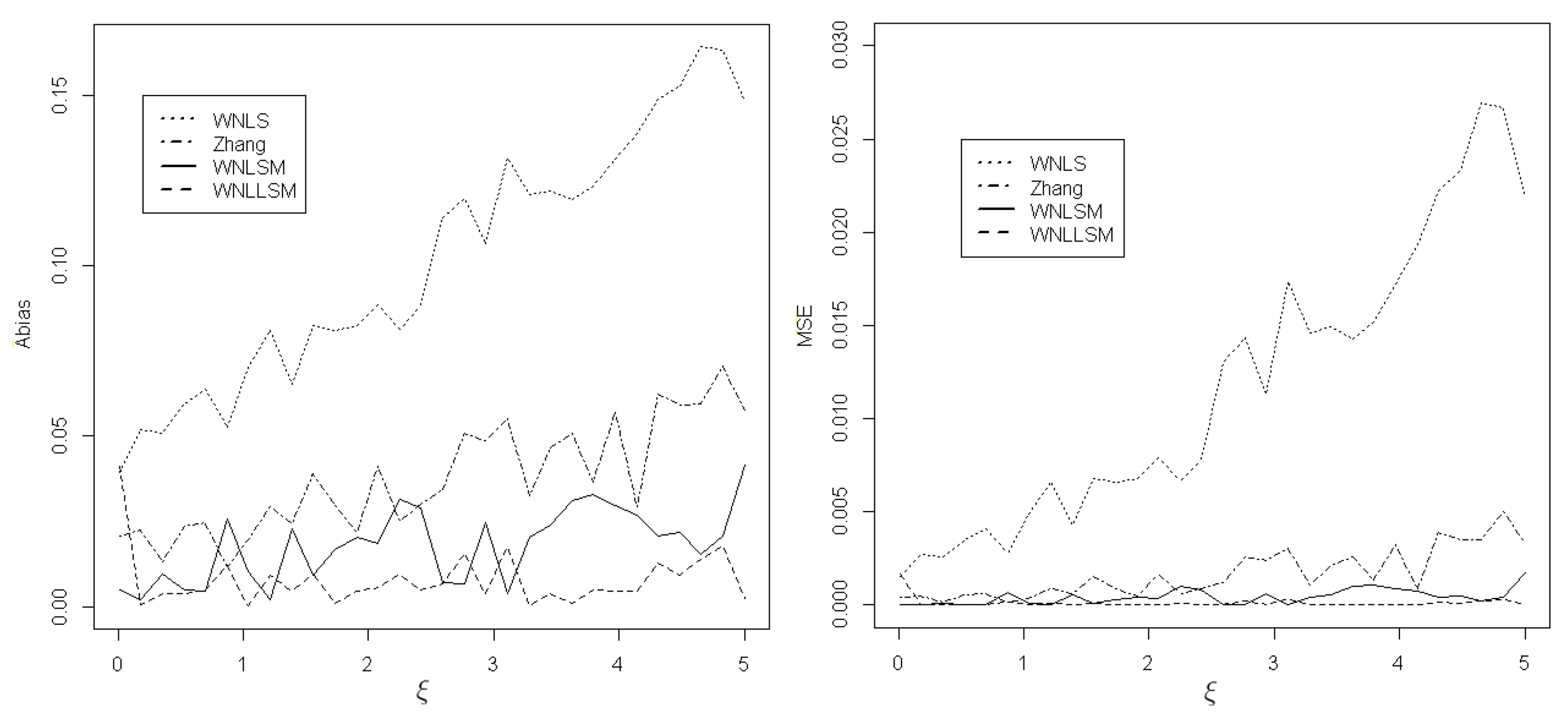
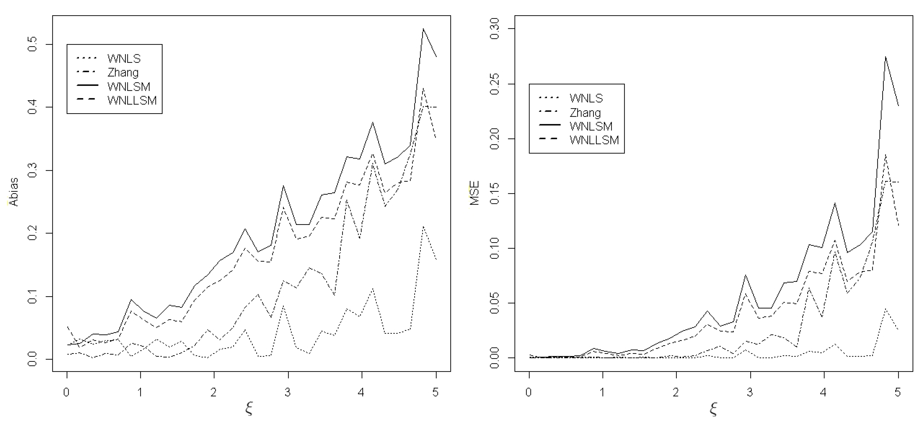
Among the two parameters, determines the tail thickness of the GPD because is the tail index [4]. Parameter characterizes the shape of the GPD, especially the shape of the tail, which is significant for fitting the extreme values. Table 1 only shows the performance of estimating and b when the shape parameter takes a certain value. To comprehensively evaluate the performance of different estimation methods, another simulation was conducted to evaluate the absolute bias (Abias) and MSE with respect to the shape parameter in a given range. In this simulation study, we vary from 0 to 5. Figure 1 and Figure 2 display the results for , , and sample size based on 1000 repetitions. Figure 1 shows that for , the WNLLSM method is the best estimator, followed by WNLSM, Zhang, and WNLS. In Figure 2, for b, Zhang and WNLS are the best estimators, followed by WNLLSM and WNLSM.
3.2. Simulation Study of the Threshold Selection
Suppose that we have a sample of size n. Without loss of generality, let . If we know the sample follows the GPD, it is unnecessary to search for the GPD threshold. While if the distribution of the sample is unknown but is in the maximum domain of attraction, we may apply the POT method to model the exceedances by the GPD. First, we can obtain the maximum likelihood estimations for the parameters of the GPD. Then, once they are estimated, the threshold can be fixed by many methods. Among them, we propose three existing procedures to find a proper threshold, as outlined below.
Method 1. ForwardStop [34]:
- (a)
- Fix , where i ranges from 1 to m, and m is a fixed positive integer.
- (b)
- Test proposed by [36], and compute the corresponding p-values .
- (c)
- Compute cutoff such thatwhere is a significance level. In this case, the selected threshold is .
Method 2. Raw Up [34]:
Begin with the order statistics where , and continue with until the threshold accepts that the data above the follows the GPD.
Method 3. Raw Down [34]:
Begin with order statistics where , and continue with until the threshold rejects that the data above the follows the GPD.
Now we turn to studying the performance of threshold selection by estimating the VaR of the GPD, denoted by
for a given threshold , where is the ratio of the observations less than and equal to . presents the 100p quantile to qualify tail risk in several fields, with p close to 1.
We compare the performance of the ForwardStop method with two competing methods, Raw Up and Raw Down [34], in terms of tail risk measures VaR. Consider a sequence of order candidate thresholds. Raw Up begins at the first threshold and chooses the lowest threshold as the optimal threshold until the GPD fits the exceedances over this threshold. In contrast, Raw Down starts from the last threshold and select the biggest one until the GPD assumption is rejected.
The simulation samples are generated from a mixture distribution of the Weibull and GPD. A similar construction to that in [34], the mixture distribution can be obtained by defining the following hazard function
where is the length of the transition period, is the hazard function of the Weibull distribution with parameters , and is the hazard function of the GPD. The transition function defined as in [34] is
This ensures that becomes a continuous hazard function. Therefore, the mixture distribution function F on of the random samples generating mechanism is
For , the mixture distribution is the Weibull distribution. Denote by the probability of data being less than and equal to u, so and means the probability of the data being greater than u. Consequently,
Then u can be expressed as
For , the mixture distribution is the GPD. Based on the construction mechanism, the GPD tail starts from . Therefore, is the real threshold for the GPD, but not u. implies the probability of exceedances over the real threshold. We can find the relation between and given as
By substituting into (16), we can find the restriction between the threshold u, the transition interval length , and the Weibull and GPD parameters:
Consider two parameter pairs for computing the VaR under , , Weibull: , GPD: with and with . Conduct 1000 simulations with sample size 200. For each sample, we estimate VaR 95%, 98%, and 99% quantiles of the mixture distribution. The optimal threshold can be selected by applying the R package “eva” [42]. The simulation results can be seen in Table 2.
In term of the MSE and bias, overall we see in Table 2 that ForwardStop forms a more stable and less sensitive rule under all conditions. In addition, ForwardStop and Raw Down procedures perform better in most cases.
3.3. Application
In this section, we illustrate the utility of the proposed method by analyzing environmental data. Beijing’s daily PM2.5 records were collected from the China National Environment Monitoring Center. The data contained 361 observations from 1 September 2016 to 28 February 2017 and 1 September 2017 to 28 February 2018. We only considered the data from autumn and winter because air pollution is more serious in these seasons in Beijing. The statistical analysis started with threshold selection, followed by obtaining the exceedances, and finally, parameter estimation. The details are listed below.
- Use Raw Up, Raw Down, and ForwardStop rules to select the appropriate thresholds , , and , respectively.
- Obtain exceedances above the chosen threshold.
- Based on the exceedances, obtain parameter estimations of and by different methods.
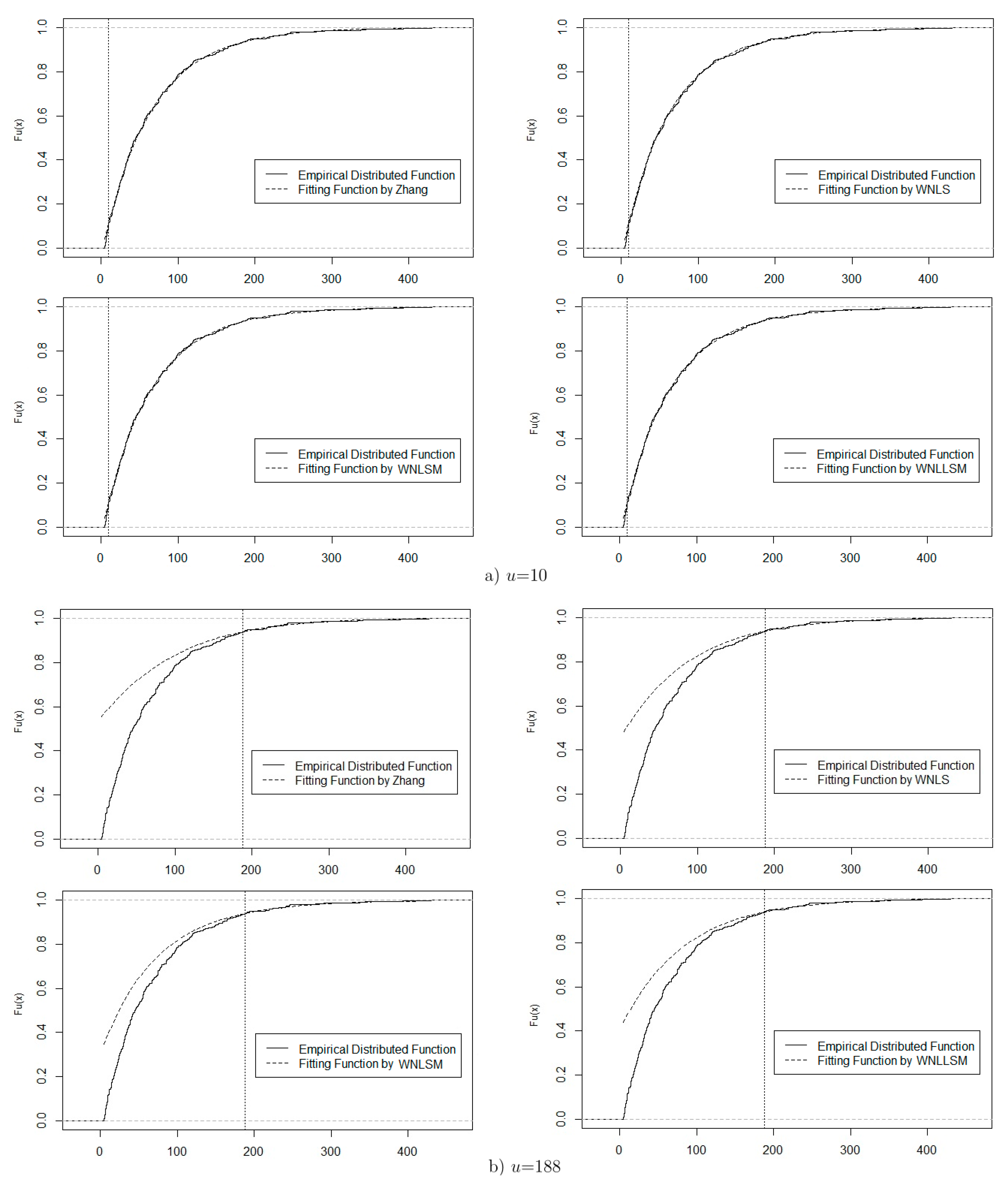
Table 3 displays the results of threshold selection and parameter and VaR estimations for the real example. In estimation, we can find by Raw Up and ForwardStop rules and by Raw Down. The predicted results can serve as references for environmental agencies and Beijing residents.
Combining the strengths of the three different threshold selection approaches, the potential thresholds are 10 and 188. For and 188, Figure 3 displays the EDF and the estimated theoretical distribution function with corresponding parameter estimators, which are shown in Table 3. Comparison plots of the EDF and theoretical distribution function are displayed in Figure 3a for and Figure 3b for , which obtained very similar results. A careful comparison of these two figures reveals that the threshold fits the data better for the GPD, especially the extreme tail, which is an important index in POT analysis.
4. Conclusions
We propose two GPD-based modeling approaches for exceedances under the POT framework. Our new methods are adapted from the recent WNLS estimator of Park and Kim (2016), which is based on the nonlinear weighted optimization of the residual squares between the distribution function and the EDF. Combining the concepts of the weighted nonlinear least squares method, the MOM, and the likelihood moments technique, we introduce the WNLSM and WNLLSM methods, which minimize the sum of squared deviations between the theoretical distribution function and its expectation. Our proposed methods are stable and provide analytical solutions. The results of extensive simulation studies demonstrate that the performance of the new estimators is highly competitive with other methods in estimating the shape parameter . We also investigate the performance of the threshold selection methods ForwardStop rule, Raw Up, and Raw Down. The simulation results show that there is not always a winner in all conditions. ForwardStop and Raw Down perform relatively better than the Raw Up procedure in most cases. However, ForwardStop is more stable to other two competing threshold selection tests. In practice, our estimations and the existing threshold selection methods are applied to daily PM2.5 data from Beijing, and the new methods produce satisfactory results in the environmental data analysis. In summary, our estimation methods are specifically designed for extreme data under the POT framework and are computationally efficient and straightforward.
Author Contributions
Data curation, X.Z. and Z.Z.; Funding acquisition, X.Z.; Methodology, X.Z. and W.C.; Project administration, X.Z.; Software, X.Z. and Z.Z.; Supervision, W.C.; Writing—original draft, X.Z. and P.Z.; Writing—review and editing, P.Z.
Funding
The authors gratefully acknowledge the support of National Natural Science Foundation of China through grant No. 11801019.
Acknowledgments
The authors would like to thank the referees and editors for their very helpful and constructive comments, which have significantly improved the quality of this paper.
Conflicts of Interest
The authors declare no conflict of interest.
Appendix A
A selected R software code is attached in the Appendix for reasons of space. More complete codes can be requested from the authors.
- #to estimate the weighted nonlinear least squares moments (WNLSM) of a
- sample X by GPD(xi, mu, sigma). For~the GPD, threshold u is equal to zero.
- sum_i <- function(i) sum(1/(n-seq(i)+1))
- WNLSM1 <- function(beta1){
- sum2 <- 0
- for (i in (nu0+1):n)
- { sum2 <- sum2 + (sum_i(i)+log(1-F0)-log(1+beta1[2]*(x[i]-u))/beta1[1]
- )^2 } #equation (10)
- sum2}
- #WNLSM1 searches for the initial WNLSM estimator (\hat(xi_1),\hat(b_1)),
- #where beta1=(xi, b), b=xi/sigma.
- WNLSM <- function(beta1){
- sum2 <- 0
- for (i in (nu0+1):n)
- {sum2 <- sum2 + ((n+1)^2*(n+2)/(i*(n-i+1)))*((i-n-1)/((n+1)*(1-F0))
- +(1+beta1[2]*(x[i]-u))^(-1/beta1[1]))^2} #equation (11)
- sum2}
- #WNLSM searches for the final WNLSM estimator (\hat(xi_2),\hat(b_2)).
- #to estimate the weighted nonlinear least squares likelihood moments
- (WNLLSM) of a sample X by GPD(xi, mu, sigma).
- WNLLSM1 <- function(b){
- sum1 <- mean(log(1+b*z))#z is the excess loss X-u|X>u and sum1=xi(b)
- #given in equation (4)
- sum2 <- 0
- for (i in (nu0+1):n){
- sum2 <- sum2 + (sum_i(i)+log(1-F0)-log(1+b*(x[i]-u))/sum1)^2}
- #equation (13)
- sum2}
- #WNLLSM1 searches for the initial WNLLSM estimator (\hat(xi_1),\hat(b_1)).
- WNLLSM <- function(b){
- sum1 <- mean(log(1+b*z)) #xi(b)
- sum2 <- 0
- for (i in (nu0+1):n){
- sum2 <- sum2 + ((n+1)^2*(n+2)/(i*(n-i+1)))*((i-n-1)/((n+1)*(1-F0))
- +(1+b*(x[i]-u))^(-1/sum1))^2} #equation (14)
- sum2}
- #WNLLSM searches for the final WNLLSM estimator (\hat(xi_2),\hat(b_2)).
- #Real data used in Section~3.3
7, 11, 18, 80, 27, 17, 41, 20, 17, 15, 32, 31, 86, 101, 69, 133, 41, 22, 10, 18, 63, 99, 121, 111, 162, 58, 24, 13, 51, 97, 165, 183, 120, 33, 55, 72, 39, 11, 31, 87, 116, 77, 150, 241, 190, 119, 59, 117, 225, 94, 42, 14, 26, 60, 96, 43, 30, 10, 23, 43, 8, 40, 99, 182, 242, 179, 71, 39, 34, 148, 130, 77, 74, 93, 42, 62, 97, 114, 188, 123, 52, 9, 7, 17, 67, 153, 254, 56, 58, 96, 89, 27, 92, 191, 246, 49, 75, 120, 91, 21, 46, 159, 219, 56, 24, 25, 101, 184, 219, 214, 365, 393, 93, 31, 117, 145, 45, 35, 57, 54, 201, 280, 430, 161, 290, 344, 224, 194, 165, 36, 32, 23, 56, 39, 7, 18, 51, 92, 132, 37, 45, 21, 25, 23, 32, 85, 171, 159, 60, 337, 39, 24, 75, 30, 80, 154, 247, 12, 12, 75, 32, 6, 6, 42, 104, 79, 176, 232, 107, 20, 83, 97, 10, 60, 76, 16, 25, 10, 27, 64, 14, 134, 109, 55, 87, 39, 14, 42, 106, 78, 90, 19, 19, 70, 86, 58, 87, 10, 21, 12, 12, 55, 24, 46, 59, 75, 48, 26, 9, 40, 107, 73, 12, 15, 53, 67, 109, 126, 29, 5, 10, 19, 35, 14, 46, 38, 68, 67, 53, 93, 75, 37, 34, 66, 106, 149,166, 47, 7, 17, 56, 63, 50, 7, 33, 98, 151, 86, 18, 50, 9, 16, 53, 26, 9, 14, 55, 24, 34, 86, 101, 119, 7, 6, 18, 39, 10, 67, 39, 12, 22, 67, 144, 52, 5, 22, 23, 8, 20, 33, 6, 5, 12, 31, 70, 35, 7, 24, 13, 34, 21, 51, 36, 30, 14, 28, 22, 75, 105, 172, 116, 29, 35, 27, 10, 14, 30, 14, 37, 12, 6, 5, 10, 55, 98, 136, 29, 45, 43, 56, 80, 30, 35, 23, 8, 15, 8, 24, 78, 13, 8, 10, 19, 30, 7, 7, 17, 6, 41, 32, 48, 41, 9, 8, 10, 55, 14, 37, 75, 78, 113, 140, 47, 32, 15, 20, 30, 54, 120, 169, 92
References
- Ferreira, A.; de Haan, L. On the block maxima method in extreme value theory: PWM estimators. Ann. Stat. 2015, 43, 276–298. [Google Scholar] [CrossRef] [Green Version]
- Rolski, T.; Schmidli, H.; Schmidt, V.; Teugel, J. Stochastic Processes for Insurance and Finance; John Wiley & Sons: Hoboken, NJ, USA, 1999. [Google Scholar]
- Daouia, A.; Girard, S.; Stupfler, G. Estimation of tail risk based on extreme expectiles. J. R. Stat. Soc. Ser. B (Stat. Methodol.) 2018, 80, 263–292. [Google Scholar] [CrossRef]
- Park, M.H.; Kim, J.H.T. Estimating extreme tail risk measures with generalized Pareto distribution. Comput. Stat. Data Anal. 2016, 98, 91–104. [Google Scholar] [CrossRef]
- Hosking, J.; Wallis, J. Parameter and quantile estimation for the Generalized Pareto distribution. Technometrics 1987, 29, 339–349. [Google Scholar] [CrossRef]
- Grimshaw, S. Computing maximum likelihood estimates for the generalized Pareto distribution. Technometrics 1993, 35, 185–191. [Google Scholar] [CrossRef]
- Greenwood, J.A.; Landwehr, J.M.; Matalas, N.C.; Wallis, J.R. Probability weighted moments: definition and relation to parameters of several distributions expressible in inverse form. Water Resour. Res. 1979, 15, 1049–1054. [Google Scholar] [CrossRef]
- Moharram, S.H.; Gosain, A.K.; Kapoor, P.N. A comparative study for the estimators of the generalized Pareto distribution. J. Hydrol. 1993, 150, 169–185. [Google Scholar]
- Castillo, E.; Hadi, A.S. Fitting the generalized Pareto distribution to data. J. Am. Stat. Assoc. 1997, 92, 1609–1620. [Google Scholar] [CrossRef]
- Arnold, B.C.; Press, S.J. Bayesian estimation and prediction for Pareto data. J. Am. Stat. Assoc. 1989, 84, 1079–1084. [Google Scholar] [CrossRef]
- de Zea Bermudez, P.; Amaral Turkman, M.A. Bayesian approach to parameter estimation of the generalized Pareto distribution. Test 2003, 12, 259–277. [Google Scholar] [CrossRef]
- Diebolt, J.; El-Aroui, M.; Garrido, M.; Girard, S. Quasi-conjugate Bayes estimates for GPD parameters and application to heavy tails modelling. Extremes 2005, 8, 57–78. [Google Scholar] [CrossRef]
- Castellanos, M.E.; Cabras, S. A default Bayesian procedure for the generalized Pareto distribution. J. Stat. Plan. Inference 2007, 137, 473–483. [Google Scholar] [CrossRef]
- Hosking, J.R.M. L-Moments: Analysis and estimation of distributions using linear combinations of order statistics. J. R. Stat. Soc. Ser. B (Methodol.) 1990, 52, 105–124. [Google Scholar] [CrossRef]
- Wang, Q.J. LH moments for statistical analysis of extreme events. Water Resour. Res. 1997, 33, 2841–2848. [Google Scholar] [CrossRef] [Green Version]
- De Zea Bermudeza, P.; Kotz, S. Parameter estimation of the generalized Pareto distribution—Part I. J. Stat. Plan. Inference 2010, 140, 1353–1373. [Google Scholar] [CrossRef]
- Rasmussen, P.F. Generalized probability weighted moments: Application to the generalized Pareto distribution. Water Resour. Res. 2001, 37, 1745–1751. [Google Scholar] [CrossRef]
- Chen, H.; Cheng, W.; Zhao, J.; Zhao, X. Parameter estimation for generalized Pareto distribution by generalized probability weighted moment-equations. Commun. Stat.-Simul. Comput. 2017, 46, 7761–7776. [Google Scholar] [CrossRef]
- Deidda, R. A multiple threshold method for fitting the generalized Pareto distribution to rainfall time series. Hydrol. Earth Syst. Sci. 2010, 14, 2559–2575. [Google Scholar] [CrossRef] [Green Version]
- Zhang, J. Likelihood moment estimation for the generalized pareto distribution. Aust. N. Z. J. Stat. 2007, 49, 69–77. [Google Scholar] [CrossRef]
- del Castillo, J.; Serra, I. Likelihood inference for generalized pareto distribution. Comput. Stat. Data Anal. 2015, 83, 116–128. [Google Scholar] [CrossRef]
- Zhang, J.; Stephens, M.A. A New and Efficient Estimation Method for the Generalized Pareto Distribution. Technometrics 2009, 51, 316–325. [Google Scholar] [CrossRef]
- Zhang, J. Improving on estimation for the generalized pareto distribution. Technometrics 2010, 52, 335–339. [Google Scholar] [CrossRef]
- Song, J.; Song, S. A quantile estimation for massive data with generalized pareto distribution. Comput. Stat. Data Anal. 2012, 56, 143–150. [Google Scholar] [CrossRef]
- Kang, S.; Song, J. Parameter and quantile estimation for the generalized Pareto distribution in peaks over threshold framework. J. Korean Stat. Soc. 2017, 46, 487–501. [Google Scholar] [CrossRef]
- Beirlant, J.; Goegebeur, Y.; Segers, J.; Teugels, J. Statistics of Extremes: Theory and Applications; John Wiley & Sons: Hoboken, NJ, USA, 2006. [Google Scholar]
- De Haan, L.; Ferreira, A. Extreme Value Theory: An Introduction; Springer Science and Business Media: Berlin/Heidelberg, Germany, 2006. [Google Scholar]
- Embrechts, P.; Klüppelberg, C.; Mikosch, T. Modelling Extremal Events for Insurance and Finance; Springer Science and Business Media: Berlin/Heidelberg, Germany, 2013. [Google Scholar]
- Kim, J.H.T.; Ahn, S.; Ahn, S. Parameter estimation of the Pareto distribution using a pivotal quantity. J. Korean Stat. Soc. 2017, 46, 438–450. [Google Scholar] [CrossRef]
- Davison, A.C.; Smith, R.L. Models for exceedances over high thresholds. J. R. Stat. Soc. Ser. B (Stat. Methodol.) 1990, 52, 393–425. [Google Scholar] [CrossRef]
- Drees, H.; de Haan, L.; Resnick, S. How to make a hill plot. Ann. Stat. 2000, 28, 254–274. [Google Scholar] [CrossRef]
- Coles, S. An Introduction to Statistical Modeling of Extreme Values, 1st ed.; Springer: Berlin/Heidelberg, Germany, 2001. [Google Scholar]
- Scarrott, C.; MacDonald, A. A review of extreme value threshold estimation and uncertainty quantification. REVSTAT Stat. J. 2012, 10, 33–60. [Google Scholar]
- Bader, B.; Yan, J.; Zhang, X.B. Automated threshold selection for extreme value analysis via ordered goodness-of-fit tests with adjustment for false discovery rate. Ann. Appl. Stat. 2018, 12, 310–329. [Google Scholar] [CrossRef]
- G’Sell, M.G.; Wager, S.; Chouldechova, A.; Tibshirani, R. Sequential selection procedures and false discovery rate control. J. R. Stat. Soc. Ser. B (Stat. Methodol.) 2016, 78, 423–444. [Google Scholar]
- Choulakian, V.; Stephens, M.A. Goodness-of-fit tests for the generalized Pareto distribution. Technometrics 2001, 43, 478–484. [Google Scholar] [CrossRef]
- Dupuis, D.J. Exceedances over high thresholds: A guide to threshold selection. Extremes 1999, 1, 251–261. [Google Scholar] [CrossRef]
- Langousis, A.; Mamalakis, A.; Puliga, M.; Deidda, R. Threshold detection for the generalized Pareto distribution: Review of representative methods and application to the NOAA NCDC daily rainfall database. Water Resour. Res. 2016, 52, 2659–2681. [Google Scholar] [CrossRef]
- Pickands, J. Statistical inference using extreme order statistics. Ann. Stat. 1975, 3, 119–131. [Google Scholar]
- Balkema, A.A.; de Haan, L. Residual life time at great age. Ann. Probab. 1974, 2, 792–804. [Google Scholar] [CrossRef]
- Shevchenko, P.V. Implementing loss distribution approach for operational risk. Appl. Stoch. Model. Bus. Ind. 2010, 26, 277–307. [Google Scholar] [CrossRef]
- Bader, B.; Yan, J. eva: Extreme Value Analysis with Goodness-of-Fit Testing, R Package Version 0.2.5; 2018. Available online: https://cran.r-project.org/web/packages/eva/index.html (accessed on 18 March 2019).
Figure 1.
Absolute bias (Abias) and MSE of for four estimators when and .

Figure 2.
Abias and MSE of b for four estimators when and .

Figure 3.
The GPD fitting plots for Beijing’s daily PM2.5 data.


Table 1.
Parameter estimation of the generalized Pareto distribution (GPD).
| n | Methods | MSE | Bias | |||
|---|---|---|---|---|---|---|
| GPD(0.5, 1) | 50 | Zhang | 0.002 | −0.044 | −0.010 | |
| MLE | 0.002 | −0.047 | −0.009 | |||
| L-moments | 0.009 | 0.005 | −0.094 | −0.070 | ||
| GPWME | 0.001 | −0.037 | 0.007 | |||
| WNLS | 0.010 | 0.001 | −0.100 | −0.035 | ||
| WNLSM | 0.010 | 0.021 | 0.100 | |||
| WNLLSM | 0.005 | −0.001 | 0.068 | |||
| 100 | Zhang | −0.022 | −0.004 | |||
| MLE | −0.023 | −0.005 | ||||
| L-moments | 0.004 | 0.002 | −0.060 | −0.048 | ||
| GPWME | 0.018 | 0.003 | ||||
| WNLS | 0.003 | −0.059 | −0.029 | |||
| WNLSM | 0.002 | 0.006 | 0.042 | |||
| WNLLSM | −0.002 | 0.030 | ||||
| 200 | Zhang | −0.011 | −0.003 | |||
| MLE | −0.011 | −0.003 | ||||
| L-moments | 0.001 | 0.001 | −0.038 | −0.032 | ||
| GPWME | −0.009 | 0.001 | ||||
| WNLS | −0.031 | −0.017 | ||||
| WNLSM | 0.002 | 0.018 | ||||
| WNLLSM | −0.002 | 0.013 | ||||
| GPD(1, 10) | 50 | Zhang | 0.002 | −0.052 | ||
| MLE | 0.002 | −0.043 | 0.002 | |||
| L-moments | 0.100 | 0.002 | −0.316 | −0.047 | ||
| GPWME | 0.002 | −0.045 | 0.001 | |||
| WNLS | 0.014 | −0.120 | −0.002 | |||
| WNLSM | 0.001 | 0.027 | 0.015 | |||
| WNLLSM | 0.004 | 0.011 | ||||
| 100 | Zhang | −0.026 | ||||
| MLE | −0.021 | 0.001 | ||||
| L-moments | 0.069 | 0.002 | −0.263 | −0.043 | ||
| GPWME | −0.022 | |||||
| WNLS | 0.004 | −0.066 | −0.002 | |||
| WNLSM | 0.011 | 0.007 | ||||
| WNLLSM | −0.003 | 0.005 | ||||
| 200 | Zhang | −0.013 | ||||
| MLE | −0.011 | |||||
| L-moments | 0.049 | 0.002 | −0.222 | −0.039 | ||
| GPWME | −0.012 | |||||
| WNLS | 0.001 | −0.037 | −0.002 | |||
| WNLSM | 0.002 | 0.003 | ||||
| WNLLSM | −0.003 | 0.002 | ||||
| GPD(2, 1) | 50 | Zhang | 0.005 | 0.003 | −0.069 | 0.058 |
| MLE | 0.002 | 0.010 | −0.045 | 0.099 | ||
| L-moments | 1.212 | 3.252 | −1.101 | −1.803 | ||
| GPWME | 0.003 | 0.003 | −0.059 | 0.051 | ||
| WNLS | 0.027 | −0.165 | 0.021 | |||
| WNLSM | 0.002 | 0.087 | 0.041 | 0.296 | ||
| WNLLSM | 0.054 | −0.004 | 0.232 | |||
| 100 | Zhang | 0.001 | −0.033 | 0.028 | ||
| MLE | 0.002 | −0.021 | 0.046 | |||
| L-moments | 1.127 | 3.387 | −1.062 | −1.840 | ||
| GPWME | −0.028 | 0.024 | ||||
| WNLS | 0.008 | −0.089 | −0.009 | |||
| WNLSM | 0.016 | 0.016 | 0.126 | |||
| WNLLSM | 0.011 | −0.003 | 0.102 | |||
| 200 | Zhang | −0.016 | 0.014 | |||
| MLE | −0.010 | 0.022 | ||||
| L-moments | 1.076 | 3.486 | −1.037 | −1.867 | ||
| GPWME | −0.014 | 0.012 | ||||
| WNLS | 0.002 | −0.048 | −0.012 | |||
| WNLSM | 0.003 | 0.006 | 0.058 | |||
| WNLLSM | 0.002 | −0.002 | 0.048 | |||
Table 2.
Value at risk (VaR) estimation under the mixture distribution.
| Method | MSE | Bias | |||||
|---|---|---|---|---|---|---|---|
| VaR 95% | VaR 98% | VaR 99% | VaR 95% | VaR 98% | VaR 99% | ||
| Mixture distribution based on the GPD(1,0.1) with | |||||||
| 0.01 | ForwardStop | 0.331 | 0.688 | 1.199 | −0.035 | 0.118 | 0.349 |
| Raw Up | 0.335 | 0.740 | 1.338 | −0.028 | 0.216 | 0.567 | |
| Raw Down | 0.368 | 0.620 | 1.018 | −0.042 | −0.034 | 0.031 | |
| 0.05 | ForwardStop | 0.328 | 0.617 | 1.009 | −0.036 | 0.004 | 0.087 |
| Raw Up | 0.329 | 0.664 | 1.136 | −0.039 | 0.100 | 0.310 | |
| Raw Down | 0.387 | 0.598 | 0.912 | −0.034 | −0.133 | −0.203 | |
| 0.1 | ForwardStop | 0.331 | 0.595 | 0.955 | −0.034 | −0.043 | −0.015 |
| Raw Up | 0.327 | 0.634 | 1.053 | −0.040 | 0.050 | 0.195 | |
| Raw Down | 0.390 | 0.601 | 0.906 | −0.030 | −0.143 | −0.232 | |
| Mixture distribution based on the GPD(1, 0.4) with | |||||||
| 0.01 | ForwardStop | 0.816 | 2.380 | 5.043 | 0.083 | 0.897 | 2.354 |
| Raw Up | 0.840 | 2.573 | 5.594 | 0.127 | 1.183 | 3.045 | |
| Raw Down | 0.840 | 1.972 | 3.926 | −0.006 | 0.096 | 0.446 | |
| 0.05 | ForwardStop | 0.782 | 2.117 | 4.346 | 0.031 | 0.469 | 1.311 |
| Raw Up | 0.816 | 2.383 | 5.086 | 0.072 | 0.839 | 2.220 | |
| Raw Down | 0.882 | 1.813 | 3.420 | −0.038 | −0.218 | −0.279 | |
| 0.1 | ForwardStop | 0.780 | 1.983 | 4.001 | 0.005 | 0.252 | 0.807 |
| Raw Up | 0.795 | 2.265 | 4.761 | 0.048 | 0.669 | 1.810 | |
| Raw Down | 0.889 | 1.812 | 3.465 | −0.042 | −0.251 | −0.324 | |
Table 3.
Threshold selection and estimation results using Beijing’s daily PM2.5 data.
| Threshold | Method | VaR | ||||
|---|---|---|---|---|---|---|
| 97% | 98% | 99% | ||||
| = = 10 | Zhang | 0.041 | 63.4 | 240.5 | 270.3 | 322.5 |
| WNLS | 0.063 | 61.4 | 241.5 | 272.7 | 327.8 | |
| WNLSM | 0.061 | 62.6 | 245.6 | 277.2 | 333.1 | |
| WNLLSM | 0.053 | 62.7 | 242.5 | 273.2 | 327.3 | |
| Zhang | −0.108 | 82.5 | 244.3 | 274.6 | 323.4 | |
| WNLS | −0.035 | 71.3 | 237.9 | 265.9 | 312.9 | |
| WNLSM | 0.058 | 79.2 | 245.3 | 279.2 | 338.9 | |
| WNLLSM | 74.6 | 240.9 | 271.2 | 322.9 | ||
© 2019 by the authors. Licensee MDPI, Basel, Switzerland. This article is an open access article distributed under the terms and conditions of the Creative Commons Attribution (CC BY) license (http://creativecommons.org/licenses/by/4.0/).
Share and Cite
MDPI and ACS Style
Zhao, X.; Zhang, Z.; Cheng, W.; Zhang, P. A New Parameter Estimator for the Generalized Pareto Distribution under the Peaks over Threshold Framework. Mathematics 2019, 7, 406. https://0-doi-org.brum.beds.ac.uk/10.3390/math7050406
AMA Style
Zhao X, Zhang Z, Cheng W, Zhang P. A New Parameter Estimator for the Generalized Pareto Distribution under the Peaks over Threshold Framework. Mathematics. 2019; 7(5):406. https://0-doi-org.brum.beds.ac.uk/10.3390/math7050406
Chicago/Turabian StyleZhao, Xu, Zhongxian Zhang, Weihu Cheng, and Pengyue Zhang. 2019. "A New Parameter Estimator for the Generalized Pareto Distribution under the Peaks over Threshold Framework" Mathematics 7, no. 5: 406. https://0-doi-org.brum.beds.ac.uk/10.3390/math7050406
Note that from the first issue of 2016, this journal uses article numbers instead of page numbers. See further details here.