A New Algorithm for Fractional Riccati Type Differential Equations by Using Haar Wavelet


1
Department of Basic Sciences, Common First Year, King Saud University, Riyadh 11451, Saudi Arabia
2
Department of Mathematics, University of Peshawar, Peshawar 25120, Pakistan
3
Department of Mathematical Sciences, UAE University, Al-Ain 15551, UAE
*
Author to whom correspondence should be addressed.
Mathematics 2019, 7(6), 545; https://0-doi-org.brum.beds.ac.uk/10.3390/math7060545
Submission received: 6 May 2019
/
Revised: 27 May 2019
/
Accepted: 30 May 2019
/
Published: 14 June 2019
(This article belongs to the Special Issue Advances in Differential and Difference Equations with Applications 2019)
Abstract
:In this paper, a new collocation method based on Haar wavelet is developed for numerical solution of Riccati type differential equations with non-integer order. The fractional derivatives are considered in the Caputo sense. The method is applied to one test problem. The maximum absolute estimated error functions are calculated, and the performance of the process is demonstrated by calculating the maximum absolute estimated error functions for a distinct number of nodal points. The results show that the method is applicable and efficient.
1. Introduction
Fractional differential equations (FDEs) are encountered in model problems in fluid flow, finance, engineering, and other areas of applications [1,2,3,4,5,6,7,8,9,10,11,12]. Fractional Riccati DE (FRDEs) arise in many fields, although discussions on the numerical methods for these equations FRDEs are rare. Homotopy perturbation technique is used by Odibat and Momani [13] for solution of FRDEs. Khader [14] used the Chebyshev finite difference technique for solution of FRDEs. Li et al. [15] used quasi-linearization technique for solution of this problem. Yuzbasi worked on numerical solutions of FRDEs through the Bernstein polynomials [16]. Yuanlu [17] find solution of nonlinear fractional differential equation using Chebyshev wavelets. Wang and Fan [18] used the second kind Chebyshev wavelet method for solving fractional differential equations. R. Taherdangkoo and M. Abdideh [19] applied wavelet transform to detect fractured zones using conventional well logs data (Case study: Southwest of Iran). We will solve these differential equations by Haar wavelet collocation method (HWCM). Some work using HWCM can be found in the references [20,21,22,23,24,25,26]. In this paper, the fractional derivative (FD) will be considered in the Caputo sense. The Caputo FD operator of order , was introduced by M. Caputo in 1967 and defined as [27,28]:
where: , Caputo FD is a linear operator,
where are constants.
For the Caputo’s derivative, we have [29,30]:
where denotes the ceiling function and For detail on Caputo derivative see [31,32], delay differential equations see [33,34] and fractional delay differential equations see [35,36].
In this paper, we will also consider the FRDE of the following form [16]:
subject to the initial condition
where is Caputo fractional derivative of the unknown function , , and are the functions defined in , is a constant describing the order of the fractional derivative. Here we will consider the case . The aim of this work is to develop HWCM for solution of FRDEs. The significant contribution of the paper is the development of a single method based on HW which can be applied to find the solution of Riccati type differential equations of fractional order.
The paper is organized as: Preliminaries and notations are given in Section 2. Numerical technique for the solution of Riccati type differential equations of fractional order based on the Haar wavelet is developed in Section 3. Error estimation and residual correction for RDEs of fractional order are given in Section 4. In Section 5, some test problem are given to check the applicability of the method. Finally, some conclusions are drawn in Section 6.
2. Preliminaries and Notations
In this section, we present some notations, definitions and preliminary facts of the fractional calculus theory which will be used.
Definition 1.
Fractional derivative is the generalization of ordinary derivative when the derivative order is not a natural number. According to Caputo, fractional derivative operator of order η for any function is given by [17]:
where is fractional number, n is a positive integer greater than η, that is , is integral value of η and , , is the Euler’s Gamma function and is defined by [37]:
where z is a positive real number.
Definition 2.
The Rieman Liouville fractional derivative operator of order η for any function is given by [17]:
Haar Wavelet
The family of Haar wavelet falls into the category of those wavelets which have compact support. The function in the Haar wavelet family is constant functions attaining the only three values 0, 1 and . These functions are discontinuous, and their derivatives of any order vanish entirely. Due to this reason, for Haar wavelet, when applying to different types of differential equations, an indirect approach is used instead of the direct approach. The Haar wavelet family for interval is defined as [38]
where
where the integer , , where M is a positive integer and the integer . The integer r represents the level of wavelet, d represents translation and f represents dilation, V is the uppermost level of resolution and and d are related as . The family of HW form orthonomal basis for , space of square integrable functions. Therefore any function can be written as a linear combination of an infinite series of Haar basis functions in the following manner
where are real numbers and known as HW coefficients. This series is terminated after finite number of terms for approximation. Hence for any unknown function we have
These integrals can be calculated using Equation (8) and are given below.
For Haar wavelet collocation method, the computational domain is discretized using the following collocation points:
3. Convergence Analysis
Suppose that is square integrable function with on , then the error norm at Jth level satisfies (16)
Here K, C are constants and M is natural number related to Jth resolution of the wavelet.
4. Numerical Results
In this section, the proposed numerical method will be developed to find the approximate solution of Riccati type differential equations of fractional order using Haar wavelet collocation method.
First, we assume that is square integrable function and therefore can be expressed as a Haar wavelet series given as follows:
Integration yields the following relation.
where . By applying the Caputo derivative definition to Riccati type differential Equation (4) of fractional order, we have
since , therefore , and we have
By applying the Haar wavelet approximations we obtain
after simplification, we have
Substituting the collocation points , we obtain the following system of nonlinear equations
The integrals in the above system are approximated using the following Haar wavelet integration formula [39]
By applying the above integral formula, we have
This system can be solved using either Newton’s method or Broyden’s method. The Jacobian of the system is given by
where
The solution of the above system gives values of the unknown coefficients . The approximate solution at the collocation points is finally calculated by substituting in Equation (18).
5. Error Estimation and Residual Correction
In this section, we will study the error estimation and residual correction for Riccati type differential equations of fractional order. The residual function is defined as
Let us define the error function as
where is exact solution. So
also
and
subtracting Equation (23) from Equation (4), we have
by using Equations (24), (26) and (27), we have
By applying the Caputo derivative definition, we have
since , therefore , and we have
where is unknown function to be determined. The initial condition for approximate solution is
so initial condition for system (5) is
Let is square integrable function and therefore can be expressed as a Haar wavelet series given as follows:
integrating we get
where is approximated by , is Haar error estimation for . Applying Haar wavelet approximations, we have
after simplification, we get
putting the collocation points (15), we obtain a system of nonlinear equations given below,
The integrals in the above system are approximated using the following Haar wavelet integration formula [39]
By applying the above integral formula, we have
The above system can be solved using either Broyden’s method or Newton’s method. The Jacobian of the system is given by
where
6. Numerical Results and Discussion
In this section, we will use the Haar wavelet collocation technique to solve fractional (arbitrary) Riccati Type differential equation. These examples are considered because closed form solutions are available for them, or they have also been solved using other numerical schemes. The Haar wavelet is implemented on the problem which has exact solution. The performance of the proposed method is very good which can be easily observed from these tables and figure.
Numerical Experiments
In this section, some test problems are considered to illustrate the efficiency of the proposed method. The implementations and testing of the above techniques are performed in MATLAB software.
Example 1.
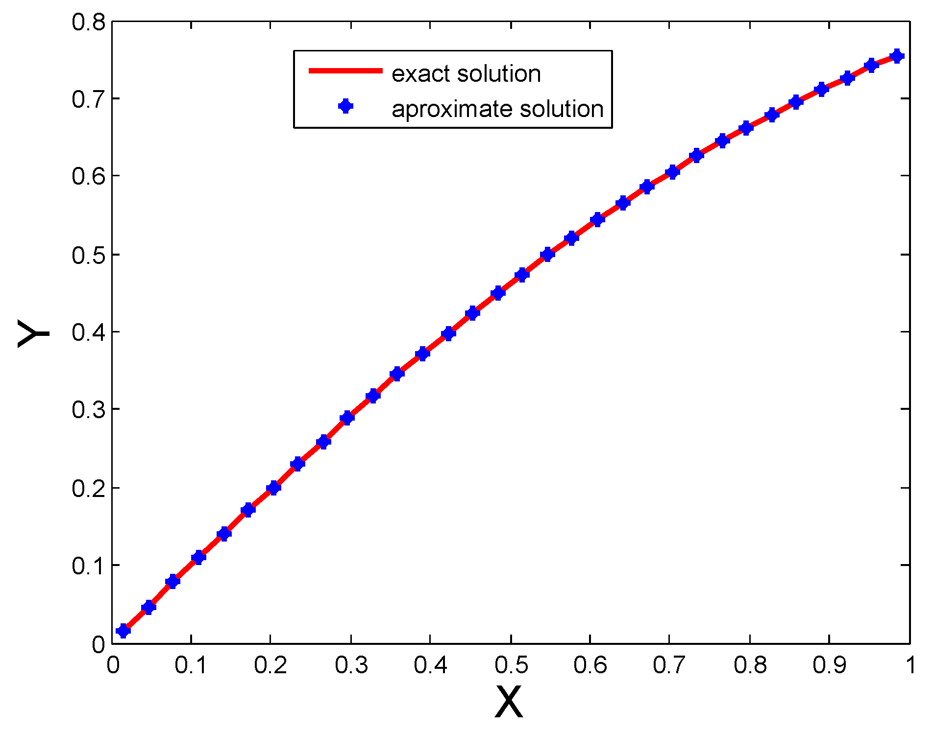
In this problem , and . The exact solution of the problem for is given by . The proposed method is applied to this nonlinear FDEs. The numerical results for are reported in Table 1, for are reported in Table 2 and for are reported in Table 3. The performance of the proposed method is very good which can be easily observed from these tables. The comparison of exact and approximate solutions for are shown in Figure 1.
Example 2.
Consider the following fractional Riccati differential equation
with initial condition
7. Conclusions
A HWCM is developed for numerical solution of FRDEs. The error estimation and residual function of this technique is given. The results show that the proposed technique is efficient and accurate. Some analytical method by using HW can be found in the references [40,41]. The performance of the method is equally suitable for these equations. By observing the tables and figures, the proposed method solutions are close to the exact solutions. Hence, the proposed technique is suitable for solving these differential equations. An excellent performance of the proposed method is observed when tested on benchmark problems of these equations from existing literature.
Author Contributions
All authors have equal contribution.
Funding
The authors would like to extend their sincere appreciation to the Deanship of Scientific Research, King Saud University for its funding through Research Unit of Common First Year Deanship.
Conflicts of Interest
The authors declare no conflicts of interest.
References
- Jafari, H.; Momani, S. Solving fractional diffusion and wave equations by modified homotopy perturbation method. Phys. Lett. A 2007, 370, 388–396. [Google Scholar] [CrossRef]
- Daftardar-Gejji, V.; Jafari, H. Solving a multi-order fractional differential equation using Adomian decomposition. Appl. Math. Comput. 2007, 189, 541–548. [Google Scholar] [CrossRef]
- Abdulaziz, O.; Hashima, I.; Momani, S. Solving systems of fractional differential equations by homotopy perturbation method. Phys. Lett. A 2008, 372, 451–459. [Google Scholar] [CrossRef]
- Podlubny, I. Geometric and physical interpretation of fractional integration and fractional differentiation. Fract. Calc. Appl. Anal. 2002, 5, 367–386. [Google Scholar]
- Morgadoa, M.L.; Ford, N.J.; Limac, P.M. Analysis and numerical methods for fractional differential equations with delay. J. Comput. Appl. Math. 2013, 252, 159–168. [Google Scholar] [CrossRef]
- Bhalekar, S.; Gejji, V.D. Fractional ordered Liu system with time-delay. Commun. Nonlinear Sci. Numer. Simul. 2010, 15, 2178–2191. [Google Scholar] [CrossRef]
- Heymans, N.; Podlubny, I. Physical interpretation of initial conditions for fractional differential equations with Riemann-Liouville fractional derivatives. Rheol. Acta 2006, 45, 765–771. [Google Scholar] [CrossRef]
- Ghasemia, M.; Kajani, M.T. Numerical solution of time-varying delay systems by Chebyshev wavelets. Appl. Math. Model. 2011, 35, 5235–5244. [Google Scholar] [CrossRef]
- Krol, K. Asymptotic properties of fractional delay differential equations. Appl. Math. Comput. 2011, 218, 1515–1532. [Google Scholar] [CrossRef] [Green Version]
- Deng, W.; Li, C.; Lu, J. Stability analysis of linear fractional differential system with multiple time delays. Nonlinear Dyn. 2007, 48, 409–416. [Google Scholar] [CrossRef]
- Chen, Y.; Moore, K.L. Analytical stability bound for a class of delayed fractional-order dynamic systems. Nonlinear Dyn. 2002, 29, 191–200. [Google Scholar] [CrossRef]
- Khader, M.M.; Hendy, A.S. The approximate and exact solutions of the fractional-order delay differential equations using Legendre pseudospectral method. Int. J. Pure Appl. Math. 2012, 74, 287–297. [Google Scholar]
- Odibat, Z.; Momani, S. Modified homotopy perturbation method: Application to quadratic Riccati differential equation of fractional order. Chaos Solitons Fractals 2008, 36, 167–174. [Google Scholar] [CrossRef]
- Khader, M.M. Numerical treatment for solving fractional Riccati differential equation. J. Egypt. Math. Soc. 2013, 21, 32–37. [Google Scholar] [CrossRef] [Green Version]
- Li, X.Y.; Wu, B.Y.; Wang, R.T. Reproducing kernel method for fractional Riccati differential equations. Abstr. Appl. Anal. 2014, 2014, 1–6. [Google Scholar] [CrossRef]
- Yuzbasi, S. Numerical solutions of fractional Riccati type differential equations by means of the Bernstein polynomials. Appl. Math. Comput. 2013, 219, 6328–6343. [Google Scholar]
- Li, Y. Solving a nonlinear fractional differential equation using Chebyshev wavelets. Commun. Nonlinear Sci. Numer. Simul. 2010, 15, 2284–2292. [Google Scholar]
- Wang, Y.; Fan, Q. The second kind Chebyshev wavelet method for solving fractional differential equations. Appl. Math. Comput. 2012, 218, 8592–8601. [Google Scholar] [CrossRef]
- Taherdangkoo, R.; Abdideh, M. Application of wavelet transform to detect fractured zones using conventional well logs data (Case study: Southwest of Iran). Int. J. Pet. Eng. 2016, 2, 125–139. [Google Scholar] [CrossRef]
- Aziz, I.; Islam, S.; Khan, W. Quadrature rules for numerical integration based on Haar wavelets and hybrid functions. Comput. Math. Appl. 2011, 61, 2770–2781. [Google Scholar] [CrossRef] [Green Version]
- Aziz, I.; Islam, S.; Sarler, B. Wavelet collocation method for the numerical solution of elliptic boundary value problems. Appl. Math. Model. 2013, 37, 676–694. [Google Scholar] [CrossRef]
- Islam, S.; Aziz, I.; Sarler, B. The numerical solution of second order boundary value problems by collocations method with Haar wavelet. Math. Comput. Model. 2010, 52, 1577–1590. [Google Scholar] [CrossRef]
- Islam, S.; Sarler, B.; Aziz, I.; Haq, F. Haar wavelet collocation method for the numerical solution of boundary layer fuid flow problems. Int. J. Therm. Sci. 2011, 50, 686–697. [Google Scholar] [CrossRef]
- Islam, S.; Aziz, I.; Fhaid, A.; Shah, A. A numerical solution of parabolic partial differential equations using Haar wavelet and Legendre wavelets. Appl. Math. Model. 2013, 37, 9455–9481. [Google Scholar] [CrossRef]
- Aziz, I.; Islam, S. New alogrithm for the numerical solution of nonlinear Fredholam and Volterra integral equations using Haar wavelet. J. Comput. Appl. Math. 2013, 239, 333–345. [Google Scholar] [CrossRef]
- Lepik, U. Solving fractional integral equations by the Haar wavelet method. Appl. Math. Comput. 2009, 214, 468–478. [Google Scholar] [CrossRef]
- Caputo, M. Linear models of dissipation whose Q is almost frequency independent. Geophys. J. Int. 1967, 13, 529–539. [Google Scholar] [CrossRef]
- Podlubny, I. Fractional Differential Equations; Academic Press: New York, NY, USA, 1999. [Google Scholar]
- Oldham, K.B.; Spanier, J. The Fractional Calculus; Academic Press: New York, NY, USA, 1974. [Google Scholar]
- Lepik, U. Numerical solution of evolution equations by the Haar wavelet method. Appl. Math. Compt. 2007, 185, 695–704. [Google Scholar] [CrossRef]
- Bellman, R.; Cooke, K.L. Differential-Difference Equations; Academic Press: London, UK, 1963. [Google Scholar]
- Kilbas, A.A.; Srivastava, H.M.; Trujillo, J.J. Theory and Applications of Fractional Differential Equations; North-Holland Mathematics Studies; Elsevier: Amsterdam, The Netherlands, 2006. [Google Scholar]
- Bellen, A.; Zennaro, M. Numerical Methods for Delay Differential Equations; Oxford University Press: Oxford, UK, 2003. [Google Scholar]
- Datta, K.B.; Mohan, B.M. Orthogonal Functions in Systems and Control; World Scientific: Singapore, 1995. [Google Scholar]
- Diethelm, K.; Ford, N.J. Analysis of fractional differential equations. J. Math. Anal. Appl. 2002, 265, 229–248. [Google Scholar] [CrossRef]
- Samko, S.G.; Kilbas, A.A.; Marichev, O.I. Fractional Integrals and Derivatives: Theory and Applications; Gordon and Breach: Yverdon, Switzerland, 1993. [Google Scholar]
- Alquran, M.; Jaradat, H.M.; Syam, M.I. Analytical solution of the time-fractional Phi-4 equation by using modified residual power series method. Nonlinear Dyn. 2017, 90, 2525–2529. [Google Scholar] [CrossRef]
- Aziz, I.; Amin, R. Numerical solution of a class of delay differential and delay partial differential equations via Haar wavelet. Appl. Math. Model. 2016, 40, 10286–10299. [Google Scholar] [CrossRef]
- Aziz, I.; Haq, F. A comparative study of numerical integration based on Haar wavelets and hybrid functions. Comput. Math. Appl. 2010, 59, 2026–2036. [Google Scholar] [CrossRef] [Green Version]
- Majak, J.; Shvartsman, B.S.; Kirs, M.; Pohlak, M.; Herranen, H. Convergence theorem for the Haar wavelet-based discretization method. Compos. Struct. 2015, 126, 227–232. [Google Scholar] [CrossRef]
- Majak, J.; Shvartsman, B.; Karjust, K.; Mikola, M.; Haavajoe, A.; Pohlak, M. On the accuracy of the Haar wavelet discretization method. Compos. Part B 2015, 80, 321–327. [Google Scholar] [CrossRef]
Figure 1.
Comparison of exact and approximate solution for for Example 1.

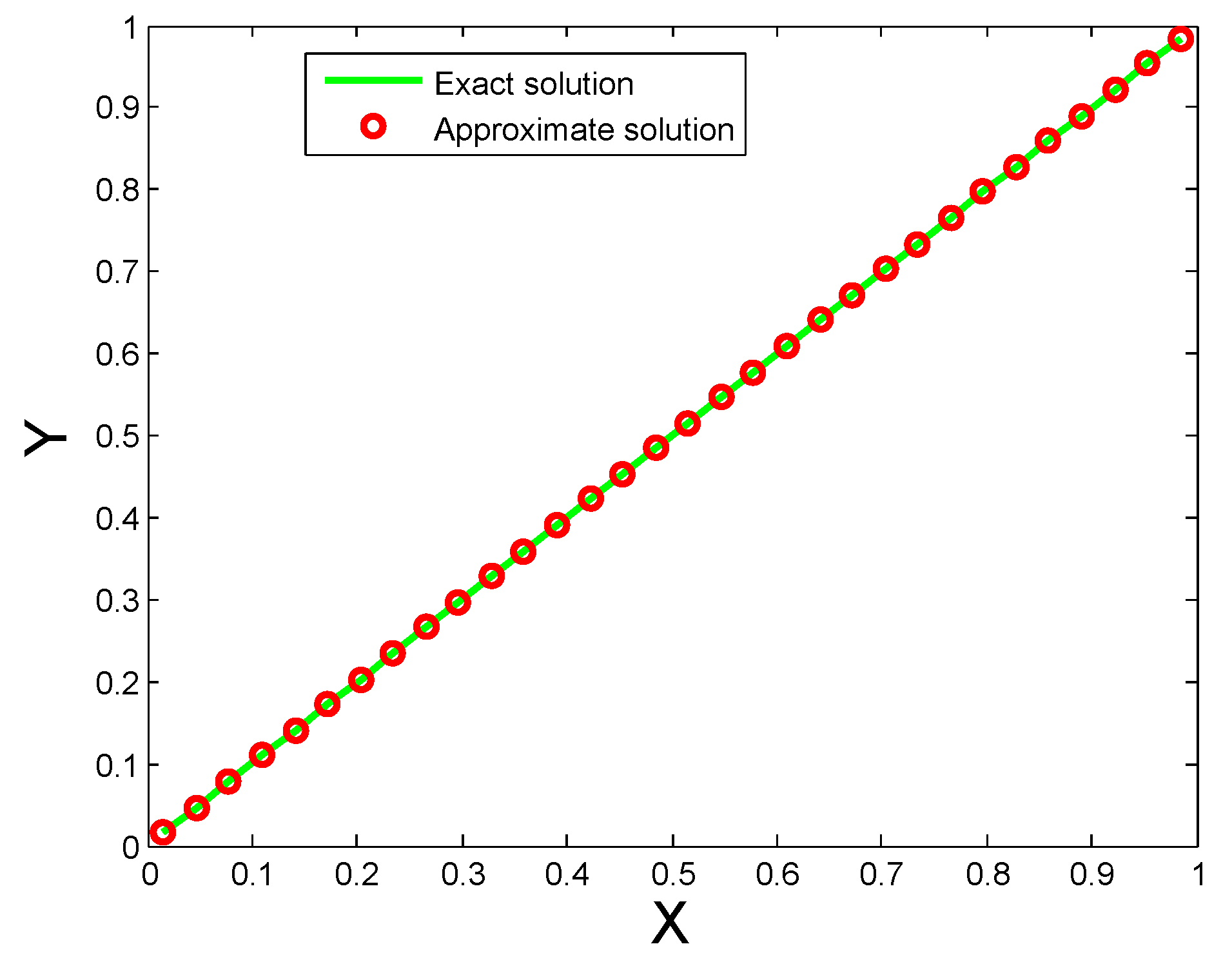
Figure 2.
Comparison of exact and approximate solution for for Example 2.


Table 1.
Maximum estimated absolute errors for for Example 1.
| J | N | M | |
|---|---|---|---|
| 1 | 4 | 8 | 4.71362 |
| 2 | 8 | 16 | 1.02141 |
| 3 | 16 | 32 | 3.72674 |
| 4 | 32 | 64 | 2.61325 |
| 5 | 64 | 128 | 4.58470 |
| 6 | 128 | 256 | 1.84356 |
| 7 | 256 | 512 | 4.01407 |
| 8 | 512 | 1024 | 1.37851 |
| 9 | 1024 | 2048 | 3.93057 |
Table 2.
Maximum estimated absolute errors for for Example 1.
| J | N | M | |
|---|---|---|---|
| 1 | 4 | 8 | 4.07815 |
| 2 | 8 | 16 | 2.08991 |
| 3 | 16 | 32 | 4.21256 |
| 4 | 32 | 64 | 2.63916 |
| 5 | 64 | 128 | 3.12723 |
| 6 | 128 | 256 | 1.61477 |
| 7 | 256 | 512 | 3.10984 |
| 8 | 512 | 1024 | 1.15074 |
| 9 | 1024 | 2048 | 4.18620 |
Table 3.
Maximum estimated absolute errors for for Example 1.
| J | N | M | |
|---|---|---|---|
| 1 | 4 | 8 | 5.86412 |
| 2 | 8 | 16 | 2.70831 |
| 3 | 16 | 32 | 3.44670 |
| 4 | 32 | 64 | 2.71416 |
| 5 | 64 | 128 | 5.50248 |
| 6 | 128 | 256 | 1.54249 |
| 7 | 256 | 512 | 5.44532 |
| 8 | 512 | 1024 | 1.13653 |
| 9 | 1024 | 2048 | 3.65001 |
Table 4.
Maximum estimated absolute errors for for Example 2.
| J | N | M | |
|---|---|---|---|
| 1 | 4 | 8 | 1.29043 |
| 2 | 8 | 16 | 3.62737 |
| 3 | 16 | 32 | 1.51488 |
| 4 | 32 | 64 | 4.07078 |
| 5 | 64 | 128 | 1.76634 |
| 6 | 128 | 256 | 5.54249 |
| 7 | 256 | 512 | 3.61688 |
| 8 | 512 | 1024 | 1.74098 |
| 9 | 1024 | 2048 | 4.80576 |
© 2019 by the authors. Licensee MDPI, Basel, Switzerland. This article is an open access article distributed under the terms and conditions of the Creative Commons Attribution (CC BY) license (http://creativecommons.org/licenses/by/4.0/).
Share and Cite
MDPI and ACS Style
Khashan, M.M.; Amin, R.; Syam, M.I. A New Algorithm for Fractional Riccati Type Differential Equations by Using Haar Wavelet. Mathematics 2019, 7, 545. https://0-doi-org.brum.beds.ac.uk/10.3390/math7060545
AMA Style
Khashan MM, Amin R, Syam MI. A New Algorithm for Fractional Riccati Type Differential Equations by Using Haar Wavelet. Mathematics. 2019; 7(6):545. https://0-doi-org.brum.beds.ac.uk/10.3390/math7060545
Chicago/Turabian StyleKhashan, M. Motawi, Rohul Amin, and Muhammed I. Syam. 2019. "A New Algorithm for Fractional Riccati Type Differential Equations by Using Haar Wavelet" Mathematics 7, no. 6: 545. https://0-doi-org.brum.beds.ac.uk/10.3390/math7060545
Note that from the first issue of 2016, this journal uses article numbers instead of page numbers. See further details here.