Some Classes of Harmonic Mapping with a Symmetric Conjecture Point Defined by Subordination

Abstract

In the paper, we introduce some subclasses of harmonic mapping, the analytic part of which is related to general starlike (or convex) functions with a symmetric conjecture point defined by subordination. Using the conditions satisfied by the analytic part, we obtain the integral expressions, the coefficient estimates, distortion estimates and the growth estimates of the co-analytic part g, and Jacobian estimates, the growth estimates and covering theorem of the harmonic function f. Through the above research, the geometric properties of the classes are obtained. In particular, we draw figures of extremum functions to better reflect the geometric properties of the classes. For the first time, we introduce and obtain the properties of harmonic univalent functions with respect to symmetric conjugate points. The conclusion of this paper extends the original research.

1. Introduction and Preliminaries

Let $\mathcal{A}$ denote the class of functions in the following form

$$h\left(z\right)=z+{\displaystyle \sum _{n=2}^{\infty }}{a}_n{z}^n,$$

(1)

where $h\left(z\right)$ is analytic in the open unit disk $\mathbb{U}=\{z\in \mathbb{C}:|z|<1\}$.

$\mathcal{S},{\mathcal{S}}^{*},\mathcal{K}$ are denoted respectively by the subclasses of $\mathcal{A}$ consisting of univalent, starlike, convex functions (for details, see [1,2]).

Let $\mathcal{P}$ denote the class of functions p satisfying $p\left(0\right)=1$ and $\mathrm{Re}p\left(z\right)>0$, where $z\in \mathbb{U}$.

The function s is subordinate to t in $\mathbb{U}$, written by $s\left(z\right)\prec t\left(z\right)$, if there exists a Schwarz function $\sigma$, analytic in $\mathbb{U}$ with $\sigma \left(0\right)=0$ and $|\sigma (z)|<1$, satisfying $s\left(z\right)=t\left(\sigma \right(z\left)\right)$(see [1]). If the function t is univalent in $\mathbb{U}$ and $s\left(z\right)\prec t\left(z\right)$, we have the equivalent results as follows,

$$s\left(0\right)=t\left(0\right)\mathrm{and}s\left(\mathbb{U}\right)\subset t\left(\mathbb{U}\right).$$

In 1994, Ma and Minda [3] introduce a class ${\mathcal{S}}^{*}\left(\varphi \right)$ of starlike functions defined by subordination, $h\left(z\right)\in {\mathcal{S}}^{*}\left(\varphi \right)$ if and only if $\frac{z{h}^{\prime }\left(z\right)}{h\left(z\right)}\prec \varphi \left(z\right)$, where $h\in \mathcal{A},\varphi \in \mathcal{P}$. The corresponding convex class $\mathcal{K}\left(\varphi \right)$ was defined in a similar way.

For $\varphi \left(z\right)=\frac{1+Az}{1+Bz}$ and $-1\le B<A\le 1$, we denote respectively the subclasses of $\mathcal{A}$ by $S^{*}(A,B)$ and $K(A,B)$ satisfying (see [4]):

$$h\in S^{*}(A,B)⟺\frac{z{h}^{\prime }\left(z\right)}{h\left(z\right)}\prec \frac{1+Az}{1+Bz}(h\in \mathcal{A},z\in \mathbb{U})$$

and

$$h\in K(A,B)⟺\frac{{\left(z{h}^{\prime }\left(z\right)\right)}^{\prime }}{h^{\prime }\left(z\right)}\prec \frac{1+Az}{1+Bz}(h\in \mathcal{A},z\in \mathbb{U}).$$

It is easy to see that $h\in K(A,B)⟺z{h}^{\prime }\left(z\right)\in S^{*}(A,B)$ and

$$K(A,B)\subset S^{*}(A,B),K(A,B)\subset K\subset \mathcal{S},S^{*}(A,B)\subset S^{*}\subset \mathcal{S}.$$

Obviously, $S^{*}(1-2\beta ,-1)=S^{*}\left(\beta \right)(0\le \beta <1)$ is a starlike function of order $\beta$ and $K(1-2\beta ,-1)=K\left(\beta \right)$ is a convex function of order $\beta$ [5]. Especially, $S^{*}(1,-1)=S^{*}$ and $K(1,-1)=K$ are well-known starlike functions and convex functions respectively.

In 1959, Sakaguchi [6] introduced the class $S_s^{*}$ of starlike functions with respect to symmetric points, $f\in S_s^{*}$ if and only if

$$\mathrm{Re}\frac{z{f}^{\prime }\left(z\right)}{f\left(z\right)-f(-z)}>0.$$

In 1987, El-Ashwa and Thomas [7] introduced some classes of starlike functions with respect to conjugate points and symmetric conjugate points satisfying the following conditions

$$\mathrm{Re}\frac{z{f}^{\prime }\left(z\right)}{f\left(z\right)+\overline{f}\left(\overline{z}\right)}>0\mathrm{and}\mathrm{Re}\frac{z{f}^{\prime }\left(z\right)}{f\left(z\right)-\overline{f}(-\overline{z})}>0.$$

In 1933, Fekete and Szegö [8] introduced a classical Fekete-Szegö problem for $f\left(z\right)=z+{\displaystyle \sum _{n=2}^{\infty }}{a}_n{z}^n\in \mathcal{S}$ as follows,

$$|a_3-\mu a_2^2|\le \left\{\begin{array}{cc}3-4\mu ,\hfill & \mu \le 0,\hfill \\ 1+2exp\left(\frac{-2\mu }{1-\mu }\right),\hfill & 0\le \mu \le 1,\hfill \\ 4\mu -3,\hfill & \mu \ge 1.\hfill \end{array}\right.$$

The result is sharp.

In 1994, Ma and Minda [3] studied the Fekete-Szegö problem of the classes of $S^{*}\left(\varphi \right)$ and $K\left(\varphi \right)$. Many authors studied the problem of Fekete-Szegö and obtained many results (see [9,10,11]).

A harmonic mapping in $\mathbb{U}$ is a complex valued harmonic function, which maps $\mathbb{U}$ onto the domain $f\left(\mathbb{U}\right)$. The mapping f has a canonical decomposition $f\left(z\right)=h\left(z\right)+\overline{g\left(z\right)}$ and h and g are analytic in $\mathbb{U}$. h is called the analytic part and g is called the co-analytic part of f. Let $S_H$ denote the class of harmonic mappings with the following form (see [12,13])

$$f=h+\overline{g},z\in \mathbb{U},$$

(2)

where

$$h\left(z\right)=z+{\displaystyle \sum _{k=2}^{\infty }}{a}_k{z}^k\mathrm{and}g\left(z\right)={\displaystyle \sum _{k=1}^{\infty }}{b}_k{z}^k,|b_1|=\alpha \in [0,1).$$

(3)

In 1936, Lewy [14] proved that f is univalent and sense-preserving in $\mathbb{U}$ if and only if $J_f\left(z\right)>0$, that is, the second complex dilatation $\omega \left(z\right)=g^{\prime }\left(z\right)/h^{\prime }\left(z\right)$ of $f\left(z\right)$ satisfying $|\omega (z)|<1$ in $\mathbb{U}$ (see [12,13]).

Many authors further investigated various subclasses of $S_H$ and obtained some important results. In [15], the authors studied the subclass of $S_H$ with $h\in \mathcal{K}$. Also, Hotta and Michalski [16] studied the properties of a subclass of $S_H$ with h is starlike and obtained the coefficient estimates, distortion estimates and growth estimates of g, and Jacobian estimates of f. Zhu and Huang [17] studied some subclasses of $S_H$ with h is convex, or starlike functions of order $\beta$ and some sharp estimates of coefficients, distortion, and growth are obtained.

According to the principle of subordination, we introduce the following general subclasses of $S_H$ of harmonic univalent starlike and convex functions with a symmetric conjecture point.

Definition 1.

Let $A,B\in \mathbb{R},-1\le B<A\le 1$. We denote the function f be in the class $H{S}_{sc}^{*,\alpha }(A,B)$ of harmonic univalent starlike functions with a symmetric conjecture point if and only if $f\in S_H$ and $h\in S_{cs}^{*}(A,B)$, that is

$$\frac{2z{h}^{\prime }\left(z\right)}{h\left(z\right)-\overline{h}(-\overline{z})}\prec \frac{1+Az}{1+Bz}.$$

(4)

Also, we denote the function f be in the class $H{K}_{sc}^{\alpha }(A,B)$ of harmonic univalent generalized convex functions with a symmetric conjecture point if and only if $f\in S_H$ and $h\in K_{sc}(A,B)$, that is

$$\frac{2{\left(z{h}^{\prime }\left(z\right)\right)}^{\prime }}{{(h\left(z\right)-\overline{h}(-\overline{z}))}^{\prime }}\prec \frac{1+Az}{1+Bz},$$

(5)

we know that $h\in K_{cs}(A,B)⟺z{h}^{\prime }\in S_{cs}^{*}(A,B)$. Additionally, we define the classes

$$H{S}_{sc}^{*}(A,B)=\bigcup _{\alpha \in [0,1)}H{S}_{sc}^{*,\alpha }(A,B)\mathit{and}H{K}_{sc}(A,B)=\bigcup _{\alpha \in [0,1)}H{K}_{sc}^{\alpha }(A,B).$$

(6)

It is clear $H{K}_{sc}^{\alpha }(A,B)\subset H{S}_{sc}^{*,\alpha }(A,B)$ and $H{K}_{sc}(A,B)\subset H{S}_{sc}^{*}(A,B).$ Especially, let $S_{cs}^{*}(1,-1)=S_{cs}^{*}$, $K_{cs}(1,-1)=K_{cs}$, $H{S}_{sc}^{*,\alpha }(1,-1)=H{S}_{sc}^{*,\alpha }$, $H{K}_{sc}^{\alpha }(1,-1)=H{K}_{sc}^{\alpha }$, $S_{cs}^{*}(1,1-2\beta )=S_{cs}^{*}\left(\beta \right)$, $K_{cs}(1,1-2\beta )=K_{cs}\left(\beta \right)$, $H{S}_{sc}^{*,\alpha }(1,1-2\beta )=H{S}_{sc}^{*,\alpha }\left(\beta \right)$, $H{K}_{sc}^{\alpha }(1,1-2\beta )=H{K}_{sc}^{\alpha }\left(\beta \right),\beta \in [0,1)$.

In order to prove our results, we need the following Lemmas.

Lemma 1.

[18] If the function $\omega \left(z\right)=c_0+c_{1}z+\dots +c_n{z}^n+\dots$ is analytic with $|\omega (z)|\le 1$ in $\mathbb{U}$, then

$$|c_n|\le 1-|c_0{|}^2,n=1,2,\dots ,$$

(7)

and

$$|c_2-\gamma c_1^2|\le max\{1,|\gamma |\}.$$

(8)

Lemma 2.

Let $-1\le B<A\le 1,n=2,3,\cdots$ . (1) If $h\left(z\right)=z+{\displaystyle \sum _{n=2}^{\infty }}{a}_n{z}^n\in S_{sc}^{*}(A,B),$ then

$$|a_{2n}|\le F_n(A,B)\mathit{and}|a_{2n+1}|\le F_n(A,B),$$

(9)

where

$$F_n(A,B)=\frac{{\displaystyle \prod _{k=0}^{n-1}}(A-B+2k)}{\left(2n\right)!!}.$$

(10)

Specially, $F_1(A,B)=\frac{A-B}{2},F_n(1,-1)=1$. The estimate is sharp if

$$h\left(z\right)={\int }_0^z\frac{1+(A-B-1)t}{(1-t)(1-t^2)\frac{A-B}{2}}dt.$$

(2) If $h\left(z\right)=z+{\displaystyle \sum _{n=2}^{\infty }}{a}_n{z}^n\in K_{sc}(A,B),$ then

$$|a_{2n}|\le \frac{F_n(A,B)}{2n}\mathit{and}|a_{2n+1}|\le \frac{F_n(A,B)}{2n+1},$$

(11)

where $F_n(A,B)$ is defined by (10). The estimate is sharp if

$$h\left(z\right)={\int }_0^z\frac{1}{\eta }{\int }_0^{\eta }\frac{1+(A-B-1)t}{(1-t)(1-t^2)\frac{A-B}{2}}dtd\eta .$$

Especially, if $A=1,B=-1$, we have the following results. (i) If $h\left(z\right)=z+{\displaystyle \sum _{n=2}^{\infty }}{a}_n{z}^n\in S_{sc}^{*},$ then

$$|a_{2n}|\le 1\mathit{and}|a_{2n+1}|\le 1.$$

(12)

The estimate is sharp if $h\left(z\right)=\frac{z}{1-z}$. (ii) If $h\left(z\right)=z+{\displaystyle \sum _{n=2}^{\infty }}{a}_n{z}^n\in K_{sc},$ then

$$|a_{2n}|\le \frac{1}{2n}\mathit{and}|a_{2n+1}|\le \frac{1}{2n+1}.$$

(13)

The estimate is sharp if $h\left(z\right)=-log(1-z)$.

Proof. 

Let $h\left(z\right)=z+{\displaystyle \sum _{n=2}^{\infty }}{a}_n{z}^n\in S_{sc}^{*}(A,B)$, there exists a positive real function $p\left(z\right)=1+{\displaystyle \sum _{k=1}^{\infty }}{p}_k{z}^k\in \mathcal{P}$ with $|p_k|\le A-B$, satisfying

$$\frac{2z{h}^{\prime }\left(z\right)}{h\left(z\right)-\overline{h}(-\overline{z})}=p\left(z\right).$$

(14)

Comparing the coefficients of the both sides of the Equation (14), we have

$$2n{a}_{2n}=p_{2n-1}+a_3{p}_{2n-3}+\cdots +a_{2n-1}{p}_1,$$

(15)

and

$$2n{a}_{2n+1}=p_{2n}+a_3{p}_{2n-2}+\cdots +a_{2n-1}{p}_2.$$

(16)

It is easy to verify that

$$|a_{2n}|\le \frac{(A-B)}{2n}(1+|a_3|+\cdots +|a_{2n-1}|)$$

(17)

and

$$|a_{2n+1}|\le \frac{(A-B)}{2n}(1+|a_3|+\cdots +|a_{2n-1}|).$$

(18)

Let $\varphi \left(n\right)=1+|a_3|+\cdots +|a_{2n-1}|$, from (18), we have

$$\varphi (n+1)\le \frac{{\displaystyle \prod _{k=1}^n}(A-B+2k)}{\left(2n\right)!!}.$$

(19)

According to (17)–(19), we can obtain (9).

If $h\left(z\right)=z+{\displaystyle \sum _{n=2}^{\infty }}{a}_n{z}^n\in K_{sc}(A,B)$, then $z{h}^{\prime }\left(z\right)\in S_{sc}^{*}(A,B)$. Using the results in (1), we can obtain (11) easily. ☐

Lemma 3.

Let $A,B\in \mathbb{R},-1\le B<A\le 1.$ (1) If $h\left(z\right)=z+{\displaystyle \sum _{n=2}^{\infty }}{a}_n{z}^n\in S_{sc}^{*}(A,B),\mu \in \mathbb{C},$ then

$$|a_3-\mu a_2^2|\le \frac{A-B}{2}max\left\{1,\left|B+\frac{\mu (A-B)}{2}\right|\right\}.$$

(20)

(2) If $h\left(z\right)=z+{\displaystyle \sum _{n=2}^{\infty }}{a}_n{z}^n\in K_{sc}(A,B),\mu \in \mathbb{C},$ then

$$|a_3-\mu a_2^2|\le \frac{A-B}{6}max\left\{1,\left|B+\frac{3\mu (A-B)}{8}\right|\right\}.$$

(21)

Proof. 

Let $h\left(z\right)=z+{\displaystyle \sum _{n=2}^{\infty }}{a}_n{z}^n\in S_{sc}^{*}(A,B)$. By definition 1 and the relationship of subordination, we have

$$\frac{2z{h}^{\prime }\left(z\right)}{h\left(z\right)-\overline{h}(-\overline{z})}=\frac{1+A\nu \left(z\right)}{1+B\nu \left(z\right)},$$

(22)

where $\nu \left(z\right)=c_{1}z+c_2{z}^2+\cdots$ is analytic in $\mathbb{U}$ satisfying $\nu \left(0\right)=0$ and $|\nu (z)|<1$.

Comparing the coefficients of the both sides of (22), we obtain

$$a_2=\frac{A-B}{2}{c}_1\mathrm{and}{a}_3=\frac{A-B}{2}{c}_2-\frac{(A-B)B}{2}{c}_1^2.$$

Therefore, we have

$$a_3-\mu a_2^2=\frac{A-B}{2}\left\{c_2-\left(B+\frac{\mu (A-B)}{2}\right)c_1^2\right\}.$$

By an application of (8) in Lemma 1, we obtain (20).

The bound is sharp as follows,

$$h\left(z\right)={\int }_0^z(1+A\xi ){(1-B\xi )}^{\frac{A-B}{2B}}{(1+B\xi )}^{\frac{A-3B}{2B}}d\xi$$

or

$$h\left(z\right)={\int }_0^z(1+A{\xi }^2){(1+B{\xi }^2)}^{\frac{A-3B}{2B}}d\xi .$$

If $h\left(z\right)=z+{\displaystyle \sum _{n=2}^{\infty }}{a}_n{z}^n\in K_{sc}(A,B)$, then $z{h}^{\prime }\left(z\right)\in S_{sc}^{*}(A,B)$. It is easy to obtain (21) and the bound is sharp as follows,

$$h\left(z\right)={\int }_0^z\frac{1}{\eta }{\int }_0^{\eta }(1+A\xi ){(1-B\xi )}^{\frac{A-B}{2B}}{(1+B\xi )}^{\frac{A-3B}{2B}}d\xi d\eta$$

or

$$h\left(z\right)={\int }_0^z\frac{1}{\eta }{\int }_0^{\eta }(1+A{\xi }^2){(1+B{\xi }^2)}^{\frac{A-3B}{2B}}d\xi d\eta .$$

☐

Lemma 4.

Let $h\left(z\right)\in \mathcal{A},$ $0\le \beta <1,|z|=r\in [0,1).$ (1) If $h\left(z\right)\in {\mathcal{S}}^{*}\left(\beta \right),$ then

$$(1-(1-2\beta )r){(1+r)}^{2\beta -3}\le |h^{\prime }\left(z\right)|\le (1+(1-2\beta )r){(1-r)}^{2\beta -3},$$

(23)

and ([4], Theorem 4 with A = 1 − 2β, B = −1)

$$r{(1+r)}^{2\beta -2}\le |h\left(z\right)|\le r{(1-r)}^{2\beta -2},$$

(24)

(2) If $h\left(z\right)\in \mathcal{K}\left(\beta \right),$ then ([19], Theorem 1 with b = 1, A = 1 − 2β, B = −1)

$${(1+r)}^{2\beta -2}\le |h^{\prime }\left(z\right)|\le {(1-r)}^{2\beta -2},$$

(25)

and ([19], Theorem 2 with b = 1, A = 1 − 2β, B = −1)

$$r{(1+r)}^{\beta -1}\le |h\left(z\right)|\le r{(1-r)}^{\beta -1}.$$

(26)

Proof. 

It suffices to establish the estimate of (23). If $h\left(z\right)\in S^{*}\left(\beta \right)$, then

$$\frac{1-(1-2\beta )r}{1+r}\le |\frac{z{h}^{\prime }\left(z\right)}{h\left(z\right)}|\le \frac{1+(1-2\beta )r}{1-r},$$

that is,

$$\frac{1-(1-2\beta )r}{1+r}|h\left(z\right)|\le |z{h}^{\prime }\left(z\right)|\le \frac{1+(1-2\beta )r}{1-r}|h\left(z\right)|.$$

According to (24), it is not difficult to verify the estimate of (23).

Using the same argument as in the proof of Lemma 2 in [20], we obtain immediately a Lemma as follows. ☐

Lemma 5.

If $h\left(z\right)\in {\mathcal{S}}_{sc}^{*}\left(\beta \right),0\le \beta <1$, then $\frac{h\left(z\right)-\overline{h}(-\overline{z})}{2}\in {\mathcal{S}}^{*}\left(\beta \right)$. Especially for $\beta =0$, we get the results of Lemma 2 in [20].

Lemma 6.

If $h\left(z\right)\in {\mathcal{K}}_{sc}\left(\beta \right),0\le \beta <1$, then $\frac{h\left(z\right)-\overline{h}(-\overline{z})}{2}\in \mathcal{K}\left(\beta \right)$.

Lemma 7.

Let $h\left(z\right)\in \mathcal{A},$ $0\le \beta <1,|z|=r\in [0,1).$ (1) If $h\in {\mathcal{S}}_{sc}^{*}\left(\beta \right),$ then

$$\frac{1-(1-2\beta )r}{{(1+r)}^{3-2\beta }}\le |h^{\prime }\left(z\right)|\le \frac{1+(1-2\beta )r}{{(1-r)}^{3-2\beta }}.$$

(27)

(2) If $h\in {\mathcal{K}}_{sc}\left(\beta \right),$ then

$$\frac{1}{{(1+r)}^{2-2\beta }}\le |h^{\prime }\left(z\right)|\le \frac{1}{{(1-r)}^{2-2\beta }}.$$

(28)

Proof. 

Suppose $h\left(z\right)\in {\mathcal{S}}_{sc}^{*}\left(\beta \right)$, we have

$$\frac{1-(1-2\beta )r}{1+r}\left|\frac{h\left(z\right)-\overline{h}(-\overline{z})}{2}\right|\le |z{h}^{\prime }\left(z\right)|\le \frac{1+(1-2\beta )r}{1-r}\left|\frac{h\left(z\right)-\overline{h}(-\overline{z})}{2}\right|.$$

(29)

According to Lemmas 4 and 5, we have

$$\frac{r}{{(1+r)}^{2-2\beta }}\le \left|\frac{h\left(z\right)-\overline{h}(-\overline{z})}{2}\right|\le \frac{r}{{(1-r)}^{2-2\beta }}.$$

(30)

By (29) and (30), we can obtain (27).

If $h\left(z\right)\in {\mathcal{K}}_{sc}\left(\beta \right)$, then

$$\frac{1-(1-2\beta )r}{1+r}\left|\frac{{(h\left(z\right)-\overline{h}(-\overline{z}))}^{\prime }}{2}\right|\le |{\left(z{h}^{\prime }\left(z\right)\right)}^{\prime }|\le \frac{1+(1-2\beta )r}{1-r}\left|\frac{{(h\left(z\right)-\overline{h}(-\overline{z}))}^{\prime }}{2}\right|.$$

(31)

According to Lemmas 4 and 6, we have

$${(1+r)}^{2\beta -2}\le \left|\frac{{(h\left(z\right)-\overline{h}(-\overline{z}))}^{\prime }}{2}\right|\le {(1-r)}^{2\beta -2}.$$

(32)

By (31) and (32), we get

$$[1-(1-2\beta )r]{(1+r)}^{2\beta -3}\le |{\left(z{h}^{\prime }\left(z\right)\right)}^{\prime }|\le [1+(1-2\beta )r]{(1-r)}^{2\beta -3}.$$

(33)

By (33), integrating along a radial line $\xi =t{e}^{i\theta }$, we obtained immediately,

$$|z{h}^{\prime }\left(z\right)|\le {\int }_0^r[1+(1-2\beta )t]{(1-t)}^{2\beta -3}dt=\frac{r}{{(1-r)}^{2-2\beta }}$$

For the left-hand side of (28), we note first that $z{h}^{\prime }\left(z\right)$ is univalent. Let $H\left(z\right):=z{h}^{\prime }\left(z\right),\Gamma =H\left(\right\{z:|z|=r\left\}\right)$ and let ${\xi }_1\in \Gamma$ be the nearest point to the origin. By a rotation we suppose that ${\xi }_1>0.$ Let $\gamma$ be the line segment $0\le \xi \le {\xi }_1$ and assume that $z_1=H^{-1}\left({\xi }_1\right)$ and $L=H^{-1}\left(\gamma \right).$ If $\varsigma$ is the variable of integration on L, we have that $d\xi =H^{\prime }\left(\varsigma \right)d\varsigma$ on L. Hence

$${\xi }_1={\int }_0^{{\xi }_1}d\xi ={\int }_0^{z_1}{H}^{\prime }\left(\varsigma \right)d\xi ={\int }_0^{z_1}|H^{\prime }\left(\varsigma \right)||d\xi |\ge {\int }_0^r|H^{\prime }\left(t{e}^{i\theta }\right)|dt$$

$$\ge {\int }_0^r[1-(1-2\beta )t]{(1+t)}^{2\beta -3}dr=\frac{r}{{(1+r)}^{2-2\beta }}.$$

So we complete the proof of Lemma 7. ☐

2. Main Results

Theorem 1.

If $f=h+\overline{g}\in H{S}_{sc}^{*,\alpha }(A,B),$ then $F=H+\overline{G}\in H{K}_{sc}^{\alpha }(A,B),$ where $H\left(z\right)$ and $G\left(z\right)$ satisfy the conditions $z{H}^{\prime }\left(z\right)=h\left(z\right)$ and $z{G}^{\prime }\left(z\right)=g\left(z\right),z\in \mathbb{U}.$

Proof. 

Let $f\in H{S}_{sc}^{*,\alpha }(A,B)$. According to Definition 1 and Alexander’s Theorem ([1], p. 43), the function $H\left(z\right)\in K_{sc}(A,B)$. Also, $H\left(0\right)=0,H^{\prime }\left(0\right)=\underset{z\to 0}{lim}\frac{h\left(z\right)}{z}=h^{\prime }\left(0\right)=1,$ and $|G^{\prime }\left(0\right)|=|\underset{z\to 0}{lim}\frac{g\left(z\right)}{z}|=|g^{\prime }\left(0\right)|=\alpha .$ Let $\Gamma :=[0,h(z\left)\right]\subset h\left(\mathbb{U}\right),z\in \mathbb{U}-\left\{0\right\}$, then

$$|g\left(z\right)|=\left|{\int }_{\Gamma }d(g\circ h^{-1}\left(\omega \right))\right|\le {\int }_{\Gamma }\left|\frac{d(g\circ h^{-1}\left(\omega \right))}{d\omega }\right||d\omega |<{\int }_{\Gamma }|d\omega |=|h\left(z\right)|.$$

Hence,

$$|G^{\prime }\left(z\right)|=\underset{t\to z}{lim}\left|\frac{g\left(t\right)}{t}\right|<\underset{t\to z}{lim}\left|\frac{h\left(t\right)}{t}\right|=|H^{\prime }\left(z\right)|.$$

It shows that F is a locally univalent and sense-preserving harmonic function in $\mathbb{U}$. Finally, appealing to ([15], Corollary 2.3), we conclude that $F=H+\overline{G}\in H{K}_{sc}^{\alpha }(A,B).$ ☐

Corollary 1.

If $f=h+\overline{g}\in H{S}_{sc}^{*}(A,B),$ then $F=H+\overline{G}\in H{K}_{sc}(A,B),$ where $H\left(z\right)$ and $G\left(z\right)$ satisfy the conditions $z{H}^{\prime }\left(z\right)=h\left(z\right)$ and $z{G}^{\prime }\left(z\right)=g\left(z\right),z\in \mathbb{U}.$

Next, we give the integral expressions for functions of these classes.

Theorem 2.

If $f=h+\overline{g}\in H{S}_{sc}^{*,\alpha }(A,B)$, then we have

$$f\left(z\right)={\int }_0^z\phi \left(\xi \right)d\xi +\overline{{\int }_0^z\omega \left(\xi \right)\phi \left(\xi \right)d\xi },$$

(34)

where

$$\phi \left(\xi \right)=\frac{1+A\nu \left(\xi \right)}{1+B\nu \left(\xi \right)}exp{\int }_0^{\xi }\frac{(A-B)}{2t}\left\{\frac{\nu \left(t\right)}{1+B\nu \left(t\right)}+\frac{\overline{\nu }(-\overline{t})}{1+B\overline{\nu }(-\overline{t})}\right\}dt,$$

(35)

and ω and ν are analytic in $\mathbb{U}$ satisfying $|\omega (0)|=\alpha ,\nu \left(0\right)=0,|\omega (z)|<1,|\nu (z)|<1$.

Proof. 

Let $f=h+\overline{g}\in H{S}_{sc}^{*,\alpha }(A,B)$. According to Definition 1 and the relationship of subordination, we have

$$g^{\prime }\left(z\right)=\omega \left(z\right)h^{\prime }\left(z\right),$$

(36)

and

$$\frac{2z{h}^{\prime }\left(z\right)}{h\left(z\right)-\overline{h}(-\overline{z})}=\frac{1+A\nu \left(z\right)}{1+B\nu \left(z\right)},$$

(37)

where $\omega$ and $\nu$ are analytic in $\mathbb{U}$ satisfying $\omega \left(0\right)=b_1,\nu \left(0\right)=0,|\omega \left(z\right)|<1,|\nu \left(z\right)|<1$. Substituting z by $-\overline{z}$ in (37), we get

$$\frac{-2\overline{z}{h}^{\prime }(-\overline{z})}{h(-\overline{z})-\overline{h}\left(z\right)}=\frac{1+A\nu (-\overline{z})}{1+B\nu (-\overline{z})}.$$

(38)

It follows from (37) and (38) that

$$\frac{2z{(\overline{h}\left(z\right)-h(-\overline{z}))}^{\prime }}{\overline{h}\left(z\right)-h(-\overline{z})}=\frac{1+A\nu \left(z\right)}{1+B\nu \left(z\right)}+\frac{1+A\overline{\nu }(-\overline{z})}{1+B\overline{\nu }(-\overline{z})}.$$

(39)

After integrating the both sides of the equality (39) and calculating it simply, we have

$$\frac{\overline{h}\left(z\right)-h(-\overline{z})}{2}=zexp{\int }_0^z\frac{(A-B)}{2t}\left\{\frac{\nu \left(t\right)}{1+B\nu \left(t\right)}+\frac{\overline{\nu }(-\overline{t})}{1+B\overline{\nu }(-\overline{t})}\right\}dt.$$

(40)

From (37) and (40), we have

$$h^{\prime }\left(z\right)=\frac{1+A\nu \left(z\right)}{1+B\nu \left(z\right)}exp{\int }_0^z\frac{(A-B)}{2t}\left\{\frac{\nu \left(t\right)}{1+B\nu \left(t\right)}+\frac{\overline{\nu }(-\overline{t})}{1+B\overline{\nu }(-\overline{t})}\right\}dt.$$

(41)

Integrating the both sides of the equality (41), we have

$$h\left(z\right)={\int }_0^z\frac{1+A\nu \left(\xi \right)}{1+B\nu \left(\xi \right)}exp{\int }_0^{\xi }\frac{(A-B)}{2t}\left\{\frac{\nu \left(t\right)}{1+B\nu \left(t\right)}+\frac{\overline{\nu }(-\overline{t})}{1+B\overline{\nu }(-\overline{t})}\right\}dtd\xi .$$

(42)

By (36) and (41), we can obtain

$$g\left(z\right)={\int }_0^z\omega \left(\xi \right)\left(\frac{1+A\nu \left(\xi \right)}{1+B\nu \left(\xi \right)}\right)exp{\int }_0^{\xi }\frac{(A-B)}{2t}\left\{\frac{\nu \left(t\right)}{1+B\nu \left(t\right)}+\frac{\overline{\nu }(-\overline{t})}{1+B\overline{\nu }(-\overline{t})}\right\}dtd\xi .$$

So, we complete the proof of Theorem 2. ☐

According to Theorem 2 and $h\in K_{sc}(A,B)$ if and only if $z{h}^{\prime }\left(z\right)\in S_{sc}^{*}(A,B)$, we obtain easily the following result.

Theorem 3.

Let $f\in H{K}_{sc}^{\alpha }(A,B)$, then we have

$$f\left(z\right)={\int }_0^z\frac{1}{\eta }{\int }_0^{\eta }\phi \left(\xi \right)d\xi d\eta +\overline{{\int }_0^z\frac{\omega \left(\eta \right)}{\eta }{\int }_0^{\eta }\phi \left(\xi \right)d\xi d\eta }.$$

(43)

where $\varphi \left(\xi \right)$ defined by (35), ω and ν are analytic in $\mathbb{U}$ satisfying $|\omega (0)|=\alpha ,\nu \left(0\right)=0,|\omega (z)|<1,|\nu (z)|<1$.

In the following, we will get the coefficient estimates of the classes.

Theorem 4.

Let $f=h+\overline{g}$, where h and g are given by (3) and $F_k(A,B)$ is defined by (10). If $f\in H{S}_{sc}^{*,\alpha }(A,B),$ then

$$|b_{2n}|\le \left\{\begin{array}{cc}\frac{1-{\alpha }^2}{2}+\frac{(A-B)\alpha }{2},\hfill & n=1,\hfill \\ \frac{(1-{\alpha }^2)}{2n}\left\{1+{\displaystyle \sum _{k=1}^{n-1}}(4k+1)F_k(A,B)\right\}+\alpha F_n(A,B),\hfill & n\ge 2,\hfill \end{array}\right.$$

(44)

and

$$|b_{2n+1}|\le \left\{\begin{array}{cc}\frac{1-{\alpha }^2}{3}(1+A-B)+\frac{(A-B)\alpha }{2},\hfill & n=1,\hfill \\ \frac{(1-{\alpha }^2)}{2n+1}\left\{1+{\displaystyle \sum _{k=1}^{n-1}}(4k+1)F_k(A,B)+2n{F}_n(A,B)\right\}+\alpha F_n(A,B),\hfill & n\ge 2.\hfill \end{array}\right.$$

(45)

The estimate is sharp and the extremal function is

$$f_0^{\alpha }\left(z\right)={\int }_0^z\frac{1+(A-B-1)t}{(1-t){(1-t^2)}^{\frac{A-B}{2}}}dt+\overline{{\int }_0^z\frac{(\alpha +(1-{\alpha }^2-\alpha )t)(1+(A-B-1)t)}{{(1-t)}^2{(1-t^2)}^{\frac{A-B}{2}}}dt}.$$

(46)

Specially, if $f\in H{S}_{sc}^{*,\alpha },$ then

$$|b_n|\le \frac{(n-1)(1-{\alpha }^2)}{2}+\alpha .$$

(47)

The estimate is sharp and the extremal function is

$$f_1^{\alpha }\left(z\right)=\frac{z}{1-z}+\overline{\frac{\alpha z+\frac{1}{2}(1-{\alpha }^2-2\alpha )z^2}{{(1-z)}^2}}=z+{\displaystyle \sum _{n=2}^{\infty }}{z}^n+\overline{{\displaystyle \sum _{n=1}^{\infty }}\left(\frac{(n-1)(1-{\alpha }^2)}{2}+\alpha \right)z^n}.$$

(48)

Especially, let $\alpha =0$ and $\alpha =\frac{1}{2}$ in (48) respectively, we have (i) If $f\in H{S}_{sc}^{*,0},$ then

$$|b_n|\le \frac{n-1}{2}.$$

The estimate is sharp and the extremal function is

$$f_1^0\left(z\right)=\frac{z}{1-z}+\overline{\frac{z^2}{2{(1-z)}^2}}=z+{\displaystyle \sum _{n=2}^{\infty }}{z}^n+\overline{{\displaystyle \sum _{n=1}^{\infty }}\frac{n-1}{2}{z}^n}.$$

(ii) If $f\in H{S}_{sc}^{*,\frac{1}{2}},$ then

$$|b_n|\le \frac{3n+1}{8}.$$

The estimate is sharp and the extremal function is

$$f_1^{\frac{1}{2}}\left(z\right)=\frac{z}{1-z}+\overline{\frac{4z-z^2}{8{(1-z)}^2}}=z+{\displaystyle \sum _{n=2}^{\infty }}{z}^n+\overline{{\displaystyle \sum _{n=1}^{\infty }}\frac{3n+1}{8}{z}^n}.$$

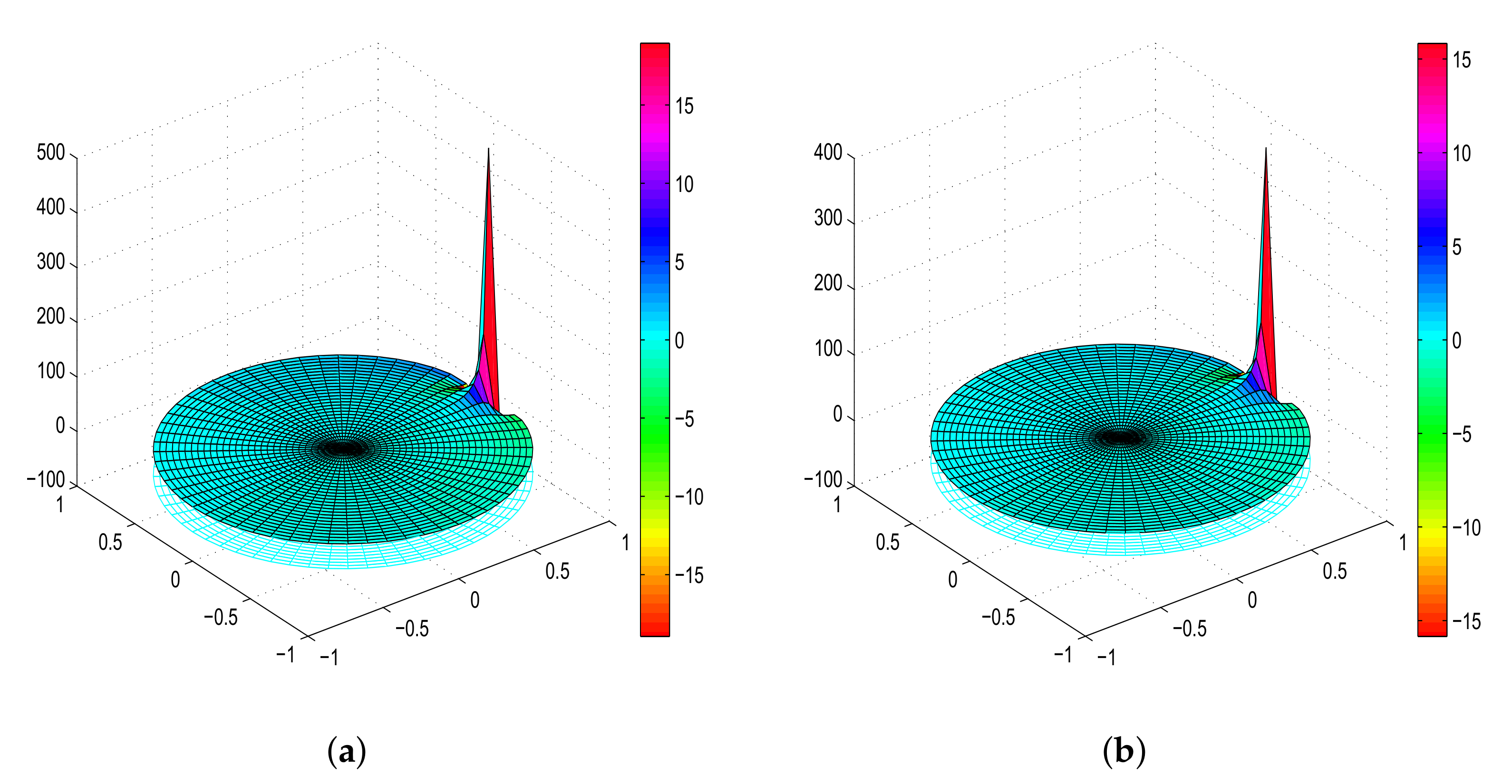
In the following Figure 1, we draw the graph of $f_1^0\left(z\right)$ and $f_1^{\frac{1}{2}}\left(z\right)$ respectively.

Proof. 

By using the relation $g^{\prime }=\omega h^{\prime }$, where h and g are given by (3) and $\omega \left(z\right)=c_0+c_{1}z+c_2{z}^2+\cdots$ is analytic in $\mathbb{U}$, we obtain

$$2n{b}_{2n}={\displaystyle \sum _{p=1}^{2n}}p{a}_p{c}_{2n-p}(a_1=1,n\ge 1)$$

(49)

and

$$(2n+1)b_{2n+1}={\displaystyle \sum _{p=1}^{2n+1}}p{a}_p{c}_{2n+1-p}(a_1=1,n\ge 1).$$

(50)

It is easy to show that

$$2n|b_{2n}|\le |c_{2n-1}|+2|a_2||c_{2n-2}|+\dots +(2n-1)|a_{2n-1}||c_1|+2n|a_{2n}||c_0|$$

(51)

and

$$(2n+1)|b_{2n+1}|\le |c_{2n}|+2|a_2||c_{2n-1}|+\dots +\left(2n\right)|a_{2n}||c_1|+(2n+1)|a_{2n+1}||c_0|.$$

(52)

Since $g^{\prime }=\omega h^{\prime }$, it follows that $c_0=b_1$. By (7), it can easily be verified that $|c_k|\le 1-{\alpha }^2,k=1,2,\cdots ,2n$. Therefore,

$$|b_{2n}|\le \left\{\begin{array}{cc}\frac{1-{\alpha }^2}{2}+|a_2|\alpha ,\hfill & n=1,\hfill \\ \frac{(1-{\alpha }^2)}{2n}(1+{\displaystyle \sum _{k=2}^{2n-1}}k|a_k|)+\alpha |a_{2n}|,\hfill & n\ge 2,\hfill \end{array}\right.$$

(53)

and

$$|b_{2n+1}|\le \left\{\begin{array}{cc}\frac{1-{\alpha }^2}{3}(1+2|a_2|)+|a_3|\alpha ,\hfill & n=1,\hfill \\ \frac{(1-{\alpha }^2)}{2n+1}(1+{\displaystyle \sum _{k=2}^{2n}}k|a_k|)+\alpha |a_{2n+1}|,\hfill & n\ge 2.\hfill \end{array}\right.$$

(54)

According to Lemma 2, (53) and (54), by simple calculation, we can obtain (44), (45) and (47). We also obtain the extreme function. Thus, the proof is completed. ☐

Using the same methods in Theorem 4, we have the following results.

Theorem 5.

Let $-1\le B<A\le 1,f=h+\overline{g}$, where h and g are given by (3) and $F_k(A,B)$ is defined by (10). If $f\in H{K}_{sc}^{\alpha }(A,B)$, then

$$|b_{2n}|\le \left\{\begin{array}{cc}\frac{1-{\alpha }^2}{2}+\frac{\alpha (A-B)}{4},\hfill & n=1,\hfill \\ \frac{(1-{\alpha }^2)}{2n}\left(1+2{\displaystyle \sum _{k=1}^{n-1}}{F}_k(A,B)\right)+\frac{\alpha }{2n}{F}_n(A,B),\hfill & n\ge 2,\hfill \end{array}\right.$$

and

$$|b_{2n+1}|\le \left\{\begin{array}{cc}\frac{(1-{\alpha }^2)}{3}(1+\frac{A-B}{2})+\frac{\alpha (A-B)}{6},\hfill & n=1,\hfill \\ \frac{(1-{\alpha }^2)}{2n+1}\left(1+2{\displaystyle \sum _{k=1}^{n-1}}{F}_k(A,B)+F_n(A,B)\right)+\frac{\alpha }{2n+1}{F}_n(A,B),\hfill & n\ge 2.\hfill \end{array}\right.$$

Specially, if $f\in H{K}_{sc}^{\alpha },n=3,4,\cdots$, then

$$|b_n|\le \frac{(n-1)(1-{\alpha }^2)}{n}+\frac{\alpha }{n}.$$

The estimate is sharp and the extremal function is

$$\begin{array}{cc}{f}_2^{\alpha }\left(z\right)& =-log(1-z)+\overline{(1-{\alpha }^2)\frac{z}{1-z}-({\alpha }^2+\alpha -1)log(1-z)}\\ & =z+{\displaystyle \sum _{n=2}^{\infty }}\frac{1}{n}{z}^n+\overline{{\displaystyle \sum _{n=1}^{\infty }}\left(\frac{(n-1)(1-{\alpha }^2)}{n}+\frac{\alpha }{n}\right)z^n}.\end{array}$$

Especially, let $\alpha =0$ and $\alpha =\frac{1}{2}$ respectively, we have (i) If $f\in H{K}_{sc}^0,$ then

$$|b_n|\le \frac{n-1}{n}$$

and the estimate is sharp and the extremal function is

$$f_2^0\left(z\right)=-log(1-z)+\overline{\frac{z}{1-z}+log(1-z)}=z+{\displaystyle \sum _{n=2}^{\infty }}\frac{1}{n}{z}^n+\overline{{\displaystyle \sum _{n=1}^{\infty }}\frac{n-1}{n}{z}^n}.$$

(ii) If $f\in H{K}_{sc}^{\frac{1}{2}}$, then

$$|b_n|\le \frac{3n-1}{4n}$$

and the estimate is sharp and the extremal function is

$$f_2^{\frac{1}{2}}\left(z\right)=-log(1-z)+\overline{\frac{3z}{4(1-z)}+\frac{1}{4}log(1-z)}=z+{\displaystyle \sum _{n=2}^{\infty }}\frac{1}{n}{z}^n+\overline{{\displaystyle \sum _{n=1}^{\infty }}\frac{3n-1}{4n}{z}^n}.$$

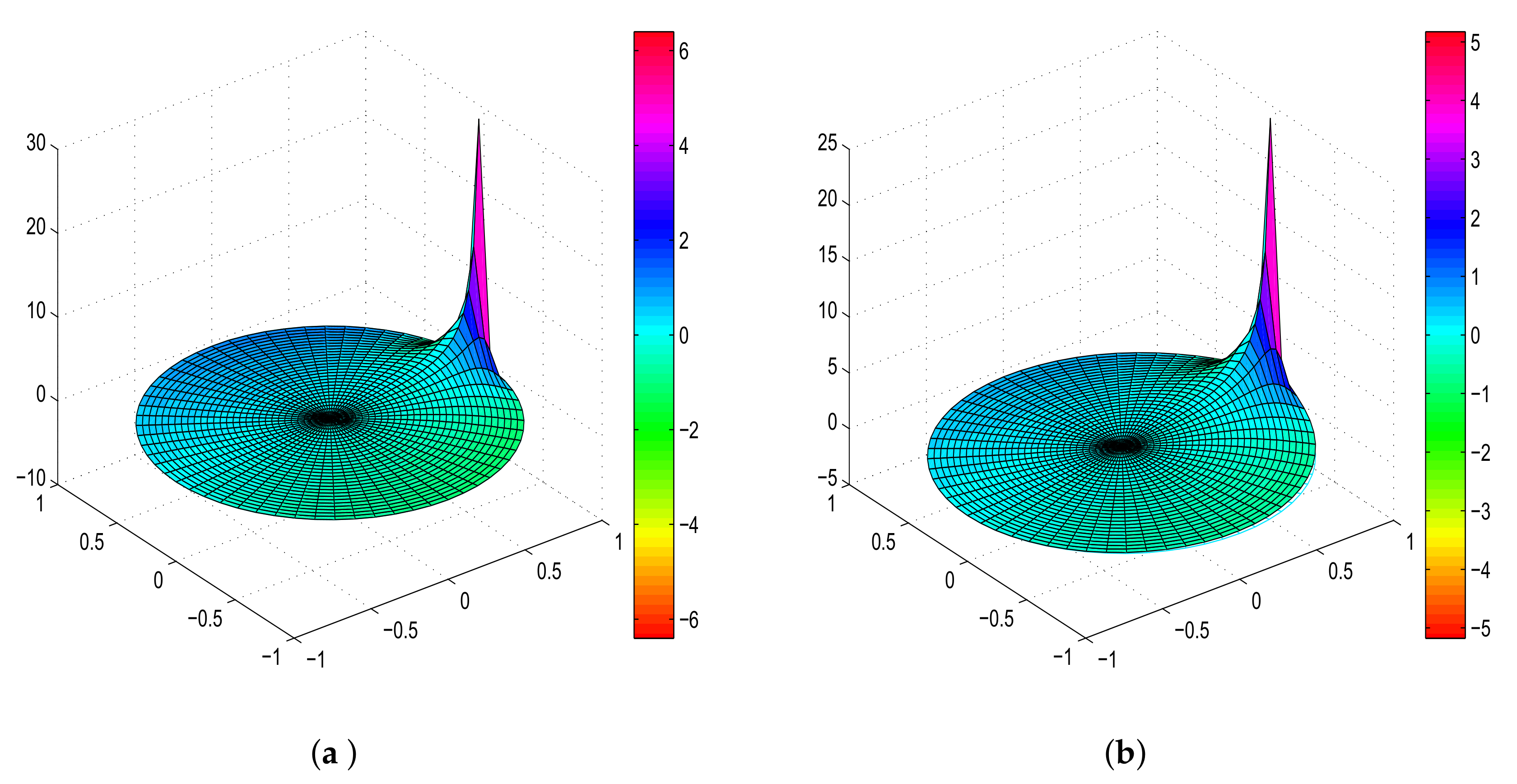
In the following Figure 2, we draw the graph of $f_2^0\left(z\right)$ and $f_2^{\frac{1}{2}}\left(z\right)$ respectively.

From Theorems 4 and 5, we have

Corollary 2.

Let $f=h+\overline{g}$, where h and g are given by (3) and $F_k(A,B)$ is defined by (10). (1) If $f\in H{S}_{sc}^{*}(A,B)$, then

$$|b_{2n}|\le \left\{\begin{array}{cc}\frac{1}{2}+\frac{{(A-B)}^2}{8},\hfill & n=1,\hfill \\ \frac{{(1+{\displaystyle \sum _{k=1}^{n-1}}(4k+1)F_k(A,B))}^2+n^2{F}_n^2(A,B)}{2n(1+{\displaystyle \sum _{k=1}^{n-1}}(4k+1)F_k(A,B))},\hfill & n\ge 2,\hfill \end{array}\right.$$

and

$$|b_{2n+1}|\le \left\{\begin{array}{cc}\frac{16+32(A-B)+25{(A-B)}^2}{48(1+A-B)},\hfill & n=1,\hfill \\ \frac{4{(1+{\displaystyle \sum _{k=1}^{n-1}}(4k+1)F_k(A,B)+2n{F}_n(A,B))}^2+{(2n+1)}^2{F}_n^2(A,B)}{4(2n+1)(1+{\displaystyle \sum _{k=1}^{n-1}}(4k+1)F_k(A,B)+2n{F}_n(A,B))},\hfill & n\ge 2.\hfill \end{array}\right.$$

Especially, if $f\in H{S}_{sc}^{*}$, then $|b_n|\le \frac{{(n-1)}^2+1}{2(n-1)}$. (2) If $f\in H{K}_{sc}(A,B)$, then

$$|b_{2n}|\le \left\{\begin{array}{cc}\frac{1}{2}+\frac{{(A-B)}^2}{32},\hfill & n=1,\hfill \\ \frac{4{(1+2{\displaystyle \sum _{k=1}^{n-1}}{F}_k(A,B))}^2+F_n^2(A,B)}{8n(1+2{\displaystyle \sum _{k=1}^{n-1}}{F}_k(A,B))},\hfill & n\ge 2,\hfill \end{array}\right.$$

and

$$|b_{2n+1}|\le \left\{\begin{array}{cc}\frac{16+16(A-B)+5{(A-B)}^2}{24(2+A-B)},\hfill & n=1,\hfill \\ \frac{4{(1+2{\displaystyle \sum _{k=1}^{n-1}}{F}_k(A,B)+F_n(A,B))}^2+F_n^2(A,B)}{4(2n+1)(1+2{\displaystyle \sum _{k=1}^{n-1}}{F}_k(A,B)+F_n(A,B))},\hfill & n\ge 2.\hfill \end{array}\right.$$

Especially, if $f\in H{K}_{sc}$, then $|b_n|\le \frac{4{(n-1)}^2+1}{4n(n-1)}$.

Also, we give the Fekete-Szegö inequality for functions of these classes.

Theorem 6.

Let $f=h+\overline{g}$, where h and g are given by (3), for $\mu \in \mathbb{C},-1\le B<A\le 1,F_n(A,B)$ is defined by (10). (1) If $f\in H{S}_{sc}^{*,\alpha }(A,B)$, then

$$\begin{array}{cc}|b_3-\mu b_2^2|\le \hfill & \frac{(1-{\alpha }^2)}{3}\left\{1+\frac{3|\mu |(1-{\alpha }^2)}{4}+\frac{(A-B)}{2}|2-3\mu b_1|\right\}+\frac{(A-B)\alpha }{2}max\left\{1,|B+\frac{\mu b_1}{2}(A-B)|\right\},\hfill \end{array}$$

(55)

$$|b_{2n}-b_{2n-1}|\le \left\{\begin{array}{cc}\frac{1}{2}(1-{\alpha }^2)+(1+\frac{A-B}{2})\alpha ,\hfill & n=1,\hfill \\ (1-{\alpha }^2)\left\{(\frac{1}{2n}+\frac{1}{2n-1})(1+{\displaystyle \sum _{k=1}^{n-1}}(4k+1)F_k(A,B))-F_{n-1}(A,B)\right\}+\hfill \\ \alpha (F_n(A,B)+F_{n-1}(A,B)),\hfill & n\ge 2,\hfill \end{array}\right.$$

(56)

and

$$\begin{array}{cc}|b_{2n+1}-b_{2n}|\le & (1-{\alpha }^2)\left\{(\frac{1}{2n+1}+\frac{1}{2n})(1+{\displaystyle \sum _{k=1}^{n-1}}(4k+1)F_k(A,B))+\frac{2n}{2n+1}{F}_n(A,B)\right\}\\ +2\alpha F_n(A,B),n\ge 1.\hfill \end{array}$$

(57)

(2) If $f\in H{K}_{sc}^{\alpha }(A,B)$, then

$$\begin{array}{c}|b_3-\mu b_2^2|\le \frac{(1-{\alpha }^2)}{3}\left\{1+\frac{3|\mu |(1-{\alpha }^2)}{4}+\frac{(A-B)}{4}|2-3\mu b_1|\right\}+\frac{(A-B)\alpha }{6}max\left\{1,|B+\frac{3(A-B)b_1\mu }{8}|\right\},\hfill \end{array}$$

(58)

$$|b_{2n}-b_{2n-1}|\le \left\{\begin{array}{cc}\frac{1}{2}(1-{\alpha }^2)+(1+\frac{A-B}{4})\alpha ,\hfill & n=1,\hfill \\ (1-{\alpha }^2)\left\{(\frac{1}{2n}+\frac{1}{2n-1})(1+2{\displaystyle \sum _{k=1}^{n-1}}{F}_k(A,B))-\frac{F_{n-1}(A,B)}{2n-1}\right\}+\hfill \\ \alpha (\frac{F_n(A,B)}{2n}+\frac{F_{n-1}(A,B)}{2n-1}),\hfill & n\ge 2,\hfill \end{array}\right.$$

(59)

and

$$\begin{array}{cc}|b_{2n+1}-b_{2n}|\le & (1-{\alpha }^2)\left\{(\frac{1}{2n+1}+\frac{1}{2n})(1+2{\displaystyle \sum _{k=1}^{n-1}}{F}_k(A,B))+\frac{1}{2n+1}{F}_n(A,B)\right\}+\\ \alpha F_n(A,B)(\frac{1}{2n+1}+\frac{1}{2n}),n\ge 1.\hfill \end{array}$$

(60)

Proof. 

From the relation (49) and (50), we have

$$2b_2=c_1+2a_2{c}_0,3b_3=c_2+2a_2{c}_1+3a_3{c}_0,$$

and

$$2n{b}_{2n}={\displaystyle \sum _{p=1}^{2n}}p{a}_p{c}_{2n-p},(2n+1)b_{2n+1}={\displaystyle \sum _{p=1}^{2n+1}}p{a}_p{c}_{2n+1-p}(a_1=1,n\ge 1).$$

By (7), we have

$$|b_3-\mu b_2^2|\le \frac{1-{\alpha }^2}{3}\left\{1+\frac{3|\mu |(1-{\alpha }^2)}{4}+|a_2||2-3\mu b_1|\right\}+\alpha \left|a_3-\mu b_1{a}_2^2\right|,$$

$$|b_{2n}-b_{2n-1}|\le \left\{\begin{array}{cc}\frac{1}{2}(1-{\alpha }^2)+\alpha (1+|a_2|),\hfill & n=1,\hfill \\ (1-{\alpha }^2)\left(\frac{1}{2n}{\displaystyle \sum _{p=1}^{2n-1}}p|a_p|+\frac{1}{2n-1}{\displaystyle \sum _{p=1}^{2n-2}}p|a_p|\right)+\alpha (|a_{2n}|+|a_{2n-1}|),\hfill & n\ge 2,\hfill \end{array}\right.$$

and

$$|b_{2n+1}-b_{2n}|\le (1-{\alpha }^2)\left(\frac{1}{2n+1}{\displaystyle \sum _{p=1}^{2n}}p|a_p|+\frac{1}{2n}{\displaystyle \sum _{p=1}^{2n-1}}p|a_p|\right)+\alpha (|a_{2n+1}|+|a_{2n}|),n\ge 1.$$

According to Lemmas 2 and 3, we can compete the proof of Theorem 6.

Especially, we let $A=1,B=-1$, we obtain the following results.

Corollary 3.

Let $f=h+\overline{g}$, where h and g are given by (3), for $\mu \in \mathbb{R}$. (1) If $f\in H{S}_{sc}^{*,\alpha }$, then

$$|b_3-\mu b_2^2|\le \frac{(1-{\alpha }^2)}{3}\left\{1+\frac{3|\mu |(1-{\alpha }^2)}{4}+|2-3\mu b_1|\right\}+\alpha max\left\{1,|b_1\mu -1|\right\},$$

(61)

and

$$|b_{n+1}-b_n|\le \frac{(2n-1)}{2}(1-{\alpha }^2)+2\alpha ,n\ge 1.$$

(62)

Especially, for $f_1^0\left(z\right)\in H{S}_{sc}^{*,0}$ given by Theorem 4, we have $|b_{n+1}-b_n|\le \frac{1}{2}$. And for $f_1^{\frac{1}{2}}\left(z\right)\in H{S}_{sc}^{*,\frac{1}{2}}$ given by Theorem 4, we have $|b_{n+1}-b_n|\le \frac{3}{8}$. (2) If $f\in H{K}_{sc}^{\alpha }$, then

$$|b_3-\mu b_2^2|\le \frac{(1-{\alpha }^2)}{3}\left\{1+\frac{3|\mu |(1-{\alpha }^2)}{4}+\frac{1}{2}|2-3\mu b_1|\right\}+\frac{\alpha }{3}max\left\{1,|\frac{3b_1\mu }{4}-1|\right\},$$

(63)

$$|b_{n+1}-b_n|\le (1-{\alpha }^2)(\frac{n}{n+1}+\frac{n-1}{n})+\alpha (\frac{1}{n+1}+\frac{1}{n}),n\ge 1.$$

(64)

Especially, for $f_2^0\left(z\right)\in H{K}_{sc}^0$ given by Theorem 5, we have $|b_{n+1}-b_n|\le \frac{1}{n(n+1)}$. And for $f_2^{\frac{1}{2}}\left(z\right)\in H{K}_{sc}^{\frac{1}{2}}$ given by Theorem 5, we have $|b_{n+1}-b_n|\le \frac{1}{4n(n+1)}$.

From Corollary 3, it is easy to obtain the following results.

Corollary 4.

Let $f=h+\overline{g}$, where h and g are given by (3). (1) If $f\in H{S}_{sc}^{*}$, then

$$|b_{n+1}-b_n|\le \left\{\begin{array}{cc}2,\hfill & n=1,\hfill \\ \frac{4n^2-4n+5}{4n-2},\hfill & n\ge 2.\hfill \end{array}\right.$$

(65)

(2) If $f\in H{K}_{sc}$, then

$$|b_{n+1}-b_n|\le \left\{\begin{array}{cc}\frac{3}{2},\hfill & n=1,\hfill \\ \frac{16n^4-12n^2+4n+5}{4n(n+1)(2n^2-1)},\hfill & n\ge 2.\hfill \end{array}\right.$$

(66)

Inspired by Zhu et al. [17], we obtain the distortion estimates and growth estimate of the co-analytic part g, Jacobian estimates, growth estimate and covering theorems of the classes of harmonic mapping with symmetric conjecture point defined by subordination as follows.

Theorem 7.

Let $f=h+\overline{g}\in S_H$, $|z|=r\in [0,1).$ (1) If $f\in H{S}_{sc}^{*,\alpha }\left(\beta \right),$ then

$$\frac{max\{\alpha -r,0\}[1-(1-2\beta \left)r\right]}{(1-\alpha r){(1+r)}^{3-2\beta }}\le |g^{\prime }\left(z\right)|\le \frac{(\alpha +r)[1+(1-2\beta \left)r\right]}{(1+\alpha r){(1-r)}^{3-2\beta }}.$$

(67)

Especially, let $\beta =0$, for $f_1^0\left(z\right)\in H{S}_{sc}^{*,0}$ given by Theorem 4, we have

$$|g^{\prime }\left(z\right)|\le \frac{r}{{(1-r)}^3}.$$

(2) If $f\in H{K}_{sc}^{\alpha }\left(\beta \right),$ then

$$\frac{max\{\alpha -r,0\}}{(1-\alpha r){(1+r)}^{2-2\beta }}\le |g^{\prime }\left(z\right)|\le \frac{(\alpha +r)}{(1+\alpha r){(1-r)}^{2-2\beta }}.$$

(68)

Especially, let $\beta =0$, for $f_2^0\left(z\right)\in H{K}_{sc}^0$ given by Theorem 5, we have

$$|g^{\prime }\left(z\right)|\le \frac{r}{{(1-r)}^2}.$$

Proof. 

According to the relation $g^{\prime }=\omega h^{\prime },|\omega \left(0\right)|=|g^{\prime }\left(0\right)|=|b_1|=\alpha$, it is easy to see $\omega \left(z\right)$ such that (see [21]):

$$|\frac{\omega \left(z\right)-\omega \left(0\right)}{1-\overline{\omega \left(0\right)}\omega \left(z\right)}|\le |z|,$$

(69)

that is,

$$|\omega \left(z\right)-\frac{\omega \left(0\right)(1-r^2)}{1-{|\omega \left(0\right)|}^2{r}^2}|\le \frac{r(1-|\omega \left(0\right){|}^2)}{1-{|\omega \left(0\right)|}^2{r}^2}.$$

(70)

From (70), we get

$$\frac{max\{\alpha -r,0\}}{1-\alpha r}\le |\omega \left(z\right)|\le \frac{\alpha +r}{1+\alpha r},z\in \mathbb{U}.$$

(71)

Applying (71) and (27), we get (67). Similarly, applying (71) and (28), we get (68). So the proof is completed. ☐

By using the same method in proof of Lemma 7, it is easy to obtain the following results.

Theorem 8.

Let $f=h+\overline{g}\in S_H$, $|z|=r\in [0,1).$ (1) If $f\in H{S}_{sc}^{*,\alpha }\left(\beta \right),$ then

$${\int }_0^r\frac{max\{\alpha -t,0\}[1-(1-2\beta \left)t\right]}{(1-at){(1+t)}^{3-2\beta }}dt\le |g\left(z\right)|\le {\int }_0^r\frac{(\alpha +t)[1+(1-2\beta \left)t\right]}{(1+\alpha t){(1-t)}^{3-2\beta }}dt.$$

(72)

Especially, let $\beta =0$, for $f_1^0\left(z\right)\in H{S}_{sc}^{*,0}$ given by Theorem 4, we have

$$|g\left(z\right)|\le \frac{r^2}{2{(1-r)}^2}.$$

(2) If $f\in H{K}_{sc}^{\alpha }\left(\beta \right),$ then

$${\int }_0^r\frac{max\{\alpha -t,0\}}{(1-\alpha t){(1+t)}^{2-2\beta }}dt\le |g\left(z\right)|\le {\int }_0^r\frac{(\alpha +t)}{(1+\alpha t){(1-t)}^{2-2\beta }}dt.$$

(73)

Especially, let $\beta =0$, for $f_2^0\left(z\right)\in H{K}_{sc}^0$ given by Theorem 5, we have

$$|g\left(z\right)|\le \frac{r}{(1-r)}+log(1-r).$$

In the following, we can obtain the Jacobian estimates and growth estimates of f.

Theorem 9.

Let $f=h+\overline{g}\in S_H$, $|z|=r\in [0,1).$ (1) If $f\in H{S}_{sc}^{*,\alpha }\left(\beta \right)$, then

$$\frac{{[1-(1-2\beta )r]}^2(1-{\alpha }^2)(1-r^2)}{{(1+r)}^{6-4\beta }{(1+\alpha r)}^2}\le J_f\left(z\right)\le \left\{\begin{array}{cc}\frac{{[1+(1-2\beta )r]}^2(1-{\alpha }^2)(1-r^2)}{{(1-r)}^{6-4\beta }{(1-\alpha r)}^2},\hfill & r<\alpha ,\hfill \\ \frac{{[1+(1-2\beta )r]}^2}{{(1-r)}^{6-4\beta }},\hfill & r\ge \alpha .\hfill \end{array}\right.$$

(2) If $f\in H{K}_{sc}^{\alpha }\left(\beta \right)$, then

$$\frac{(1-{\alpha }^2)(1-r^2)}{{(1+r)}^{4-4\beta }{(1+\alpha r)}^2}\le J_f\left(z\right)\le \left\{\begin{array}{cc}\frac{(1-{\alpha }^2)(1-r^2)}{{(1-r)}^{4-4\beta }{(1-\alpha r)}^2},\hfill & r<\alpha ,\hfill \\ \frac{1}{{(1-r)}^{4-4\beta }},\hfill & r\ge \alpha .\hfill \end{array}\right.$$

Proof. 

We know that the Jacobian of $f=h+\overline{g}$ is in the following form

$$J_f\left(z\right)=|h^{\prime }{\left(z\right)|}^2-|g^{\prime }{\left(z\right)|}^2=|h^{\prime }{\left(z\right)|}^2{(1-|\omega \left(z\right)|}^2),$$

(74)

where $\omega \left(z\right)$ is the dilatation of $f\left(z\right)$.

Let $f\in H{S}_{sc}^{*,\alpha }\left(\beta \right)$, applying (27) and (71) to (74), we obtain

$$J_f\left(z\right)\ge \frac{{[1-(1-2\beta )r]}^2}{{(1+r)}^{6-4\beta }}·\frac{(1-{\alpha }^2)(1-r^2)}{{(1+\alpha r)}^2},$$

and

$$J_f\left(z\right)\le \frac{{[1+(1-2\beta )r]}^2}{{(1-r)}^{6-4\beta }}\left(1-\frac{{(max\{(\alpha -r),0\})}^2}{{(1-\alpha r)}^2}\right)=\left\{\begin{array}{cc}\frac{{[1+(1-2\beta )r]}^2}{{(1-r)}^{6-4\beta }}·\frac{(1-{\alpha }^2)(1-r^2)}{{(1-\alpha r)}^2},\hfill & r<\alpha ,\hfill \\ \frac{{[1+(1-2\beta )r]}^2}{{(1-r)}^{6-4\beta }},\hfill & r\ge \alpha .\hfill \end{array}\right.$$

Therefore, we complete the proof of (1). Applying (28) and (71) to (74), (2) of Theorem 9 can be proved by the same method in the same way as shown before. ☐

Theorem 10.

Let $f=h+\overline{g}\in S_H$, $|z|=r,0\le r<1.$ (1) If $f\in H{S}_{sc}^{*,\alpha }\left(\beta \right),$ then

$${\int }_0^r\frac{(1-\alpha )(1-\xi )[1-(1-2\beta \left)\xi \right]}{(1+\alpha \xi ){(1+\xi )}^{3-2\beta }}d\xi \le |f\left(z\right)|\le {\int }_0^r\frac{(1+\alpha )(1+\xi )[1+(1-2\beta \left)\xi \right]}{(1+\alpha \xi ){(1-\xi )}^{3-2\beta }}d\xi .$$

(75)

(2) If $f\in H{K}_{sc}^{\alpha }\left(\beta \right),$ then

$${\int }_0^r\frac{(1-\alpha )(1-\xi )}{(1+\alpha \xi ){(1+\xi )}^{2-2\beta }}d\xi \le |f\left(z\right)|\le {\int }_0^r\frac{(1+\alpha )(1+\xi )}{(1+\alpha \xi ){(1-\xi )}^{2-2\beta }}d\xi .$$

(76)

Proof. 

For any point $z=r{e}^{i\theta }\in \mathbb{U},$ let ${\mathbb{U}}_r=\mathbb{U}(0,r)=\{z\in \mathbb{U}:|z|<r\}$ and denote

$$d=\underset{z\in {\mathbb{U}}_r}{min}|f\left({\mathbb{U}}_r\right)|,$$

(77)

and then $\mathbb{U}(0,d)\subseteq f\left({\mathbb{U}}_r\right)\subseteq f\left(\mathbb{U}\right).$ Hence, there exists $z_r\in \partial {\mathbb{U}}_r$ such that $d=|f(z_r)|.$ Let $L\left(t\right)=tf\left(z_r\right),t\in [0,1]$, then $\ell \left(t\right)=f^{-1}\left(L\left(t\right)\right),t\in [0,1]$ is a well-defined Jordan arc. For $f=h+\overline{g}\in H{S}_{sc}^{*,\alpha }\left(\beta \right),$ using (27) and (71), we have

$$\begin{array}{c}d=|f\left(z_r\right)|={\int }_L|d\omega |={\int }_{\ell }|df|={\int }_{\ell }|h^{\prime }\left(\eta \right)d\eta +\overline{g^{\prime }\left(\eta \right)}d\overline{\eta }|\hfill \\ \ge {\int }_{\ell }|h^{\prime }\left(\eta \right)|(1-|\omega \left(\eta \right)|)|d\eta |\hfill \\ \ge {\int }_{\ell }\frac{(1-\alpha )(1-|\eta |)}{1+\alpha |\eta |}·\frac{[1-(1-2\beta )|\eta |]}{{(1+|\eta |)}^{3-2\beta }}|d\eta |,\hfill \\ ={\int }_0^1\frac{(1-\alpha )(1-|\ell \left(t\right)|)}{1+\alpha |\ell (t)|}·\frac{[1-(1-2\beta )|\ell \left(t\right)|]}{{(1+|\ell \left(t\right)|)}^{3-2\beta }}dt,\hfill \\ \ge {\int }_0^r\frac{(1-\alpha )(1-\xi )}{1+\alpha \xi }·\frac{[1-(1-2\beta \left)\xi \right]}{{(1+\xi )}^{3-2\beta }}d\xi \hfill \end{array}$$

Applying (27) and (71) with a simple calculation, we can obtain the right side of (75). The remainder of the argument is analogous to that in (76) and so is omitted. ☐

According to (75) and (76), we have the following covering theorems of f.

Corollary 5.

Let $f=h+\overline{g}\in S_H$. (1) If $f\in H{S}_{sc}^{*,\alpha }\left(\beta \right),$ then $\mathbb{U}(0,R_1)\subset f\left(\mathbb{U}\right),$ where

$$R_1={\int }_0^1\frac{(1-\alpha )(1-\xi )[1-(1-2\beta \left)\xi \right]}{(1+\alpha \xi ){(1+\xi )}^{3-2\beta }}d\xi .$$

(2) If $f\in H{K}_{sc}^{\alpha }\left(\beta \right),$ then $\mathbb{U}(0,R_2)\subset f\left(\mathbb{U}\right),$ where

$$R_2={\int }_0^1\frac{(1-\alpha )(1-\xi )}{(1+\alpha \xi ){(1+\xi )}^{2-2\beta }}d\xi .$$

References

- Duren, P.L. Univalent Functions: 259 (Grundlehren der MathematischenWissenschaften); Springer: New York, NY, USA; Berlin/Heidelberg, Germany; Tokyo, Japan, 1983. [Google Scholar]
- Srivastava, H.M.; Owa, S. (Eds.) Current Topics in Analytic Function Theory; World Scientific Publishing Company: Singapore; Hackensack, NJ, USA; London, UK; Hong Kong, China, 1992. [Google Scholar]
- Ma, W.; Minda, D. A unified treatment of some special classes of univalent functions. In Proceeding of the Conference on Complex Analysis; Li, Z., Ren, F., Yang, L., Zhang, S., Eds.; International Press: Boston, MA, USA, 1994; pp. 157–169. [Google Scholar]
- Janowski, W. Some extremal problems for certain families of analytic functions. Ann. Polonici Math. 1973, 28, 297–326. [Google Scholar] [CrossRef]
- Robertso, M.I.S. On the theory of univalent functions. Ann. Math. 1936, 37, 374–408. [Google Scholar] [CrossRef]
- Sakaguchi, K. On a certain univalent mapping. J. Math. Soc. Jpn. 1959, 11, 72–75. [Google Scholar] [CrossRef]
- El-Ashwah, R.M.; Thomas, D.K. Some subclasses of closed-to-convex functions. J. Ramanujan Math. Soc. 1987, 2, 86. [Google Scholar]
- Fekete, M.; Szegö, G. Eine bemerkung uber ungerade schlichte funktionen. J. Lond. Math. Soc. 1933, 8, 85–89. [Google Scholar] [CrossRef]
- EL-Ashwah, R.M.; Hassan, A.H. Fekete-Szegö inequalities for certain subclass of analytic functions defined by using Sǎlǎgean operator. Miskolc Math. Notes 2017, 17, 827–836. [Google Scholar] [CrossRef]
- Koepf, W. On the Fekete-Szegö problem for close-to-convex functions. Proc. Am. Math. Soc. 1987, 101, 89–95. [Google Scholar]
- Sakar, F.M.; Aytaş, S.; Güney, H.Ö. On The Fekete-Szegö problem for generalized class Mα,γ(β) defined by differential operator. Süleyman Demirel Univ. J. Nat. Appl. Sci. 2016, 20, 456–459. [Google Scholar]
- Clunie, J.; Sheil-Small, T. Harmonic univalent functions. Ann. Acad. Sci. Fenn. Ser. AI Math. 1984, 39, 3–25. [Google Scholar] [CrossRef]
- Duren, P.L. Harmonic Mappings in the Plane; Cambridge University Press: Cambridge, UK, 2004. [Google Scholar]
- Lewy, H. On the non-vanishing of the Jacobian in certain one-to-one mappings. Bull. Am. Math. Soc. 1936, 42, 689–692. [Google Scholar] [CrossRef] [Green Version]
- Klimek, D.; Michalski, A. Univalent anti-analytic perturbations of convex analytic mappings in the unit disc. Ann. Univ. Mariae Curie-Skłodowska Sec. A 2007, 61, 39–49. [Google Scholar]
- Hotta, I.; Michalski, A. Locally one-to-one harmonic functions with starlike analytic part. arXiv 2014, arXiv:1404.1826. [Google Scholar]
- Zhu, M.; Huang, X. The distortion theorems for harmonic mappings with analytic parts convex or starlike functions of order β. J. Math. 2015, 2015, 460191. [Google Scholar] [CrossRef]
- Kohr, G.; Graham, I. Geometric Function Theory in one and Higher Dimensions; Marcel Dekker: New York, NY, USA, 2003. [Google Scholar]
- Polatoǧlu, Y.; Bolcal, M.; Sen, A. Two-point distortion theorems for certain families of analytic functions in the unit disc. Int. J. Math. Math. Sci. 2003, 66, 4183–4193. [Google Scholar] [CrossRef]
- Chen, M.P.; Wu, Z.R.; Zou, Z.Z. On functions α-starlike with respect to symmetric conjugate points. J. Math. Anal. Appl. 1996, 201, 25–34. [Google Scholar] [CrossRef]
- Goluzin, G.M. Geometric Theory of Functions of a Complex Variable; American Mathematical Society: Providence, RI, USA, 1969. [Google Scholar]
Figure 1.
Three dimensional coordinates plus color, the z-axis represents the real part of the function, and the color represents the imaginary part of the function. (a) The graph of ; (b) The graph of .
Figure 2.
© 2019 by the authors. Licensee MDPI, Basel, Switzerland. This article is an open access article distributed under the terms and conditions of the Creative Commons Attribution (CC BY) license (http://creativecommons.org/licenses/by/4.0/).
Share and Cite
MDPI and ACS Style
Ma, L.; Li, S.; Niu, X. Some Classes of Harmonic Mapping with a Symmetric Conjecture Point Defined by Subordination. Mathematics 2019, 7, 548. https://0-doi-org.brum.beds.ac.uk/10.3390/math7060548
AMA Style
Ma L, Li S, Niu X. Some Classes of Harmonic Mapping with a Symmetric Conjecture Point Defined by Subordination. Mathematics. 2019; 7(6):548. https://0-doi-org.brum.beds.ac.uk/10.3390/math7060548
Chicago/Turabian StyleMa, Lina, Shuhai Li, and Xiaomeng Niu. 2019. "Some Classes of Harmonic Mapping with a Symmetric Conjecture Point Defined by Subordination" Mathematics 7, no. 6: 548. https://0-doi-org.brum.beds.ac.uk/10.3390/math7060548
Note that from the first issue of 2016, this journal uses article numbers instead of page numbers. See further details here.