Numeric-Analytic Solutions for Nonlinear Oscillators via the Modified Multi-Stage Decomposition Method

Abstract

This work deals with a new modified version of the Adomian-Rach decomposition method (MDM). The MDM is based on combining a series solution and decomposition method for solving nonlinear differential equations with Adomian polynomials for nonlinearities. With application to a class of nonlinear oscillators known as the Lienard-type equations, convergence and error analysis are discussed. Several physical problems modeled by Lienard-type equations are considered to illustrate the effectiveness, performance and reliability of the method. In comparison to the 4th Runge-Kutta method (RK4), highly accurate solutions on a large domain are obtained.

1. Introduction

One of the classical equations often used to describe the development of oscillations in nonlinear mechanics, more specifically in the study of radio and vacuum tube technology, was formulated by Alfred-Marie Lienard (1869–1938) [1]. The Lienard-type equation is of the form

$$\frac{d{w}^2}{d{t}^2}+F\left(w\right)\frac{dw}{dt}+G\left(w\right)=0$$

(1)

where $F\left(w\right)$ and $G\left(w\right)$ are assumed to be analytic in $w.$ Equation (1) has been used to model the electric heart activity, neuron activity and oscillating circuits, in addition to many other models in seismology, cosmology, biology, mechanics, chemistry and physics [2].

The solution of Equation (1) exists, it is unique, and has a stable limit cycle surrounding the origin under the conditions of Lienard's theorem [1].

The Lienard’s theorem [1] establishes criteria for guaranteeing the existence, uniqueness, and stability of limit cycles surrounding the origin. As a model of oscillating circuits, Equation (1) was intensely studied. While no exact solution is known in general, several authors have devoted their attention to study whether or not the Lienard-type equations have unique periodic solutions. For examples: Écalle [3] and Ilyashenko [4] proved the existence of finitely many limit cycles with polynomial nonlinearities. Zhang et al. [5] applied the Poincaré-Bendixson theorem to generalize the previous studies. Under some restrictions on $F$, Lefschetz [6] gave an existence theorem for periodic solutions to the forced Lienard-type equation. Results of Lefschetz were systematically improved in many works [7,8,9]. On the other hand, several numeric and numeric-analytic algorithms have been employed to treat Lienard-type equations of integer and fraction derivatives.

Among these attempts are the harmonic balance, the elliptic Lindstedt-Poincare and the multiple scales methods [10], He’s parameter-expanding methods [11], He’s variational iteration method [12,13], the homotopy perturbation method [14], the differential and reduced differential transform methods [15,16,17], the Adomian decomposition method and its variants [18,19,20,21], and the residual power series method [22,23,24,25].

Main motivation of this analysis is to construct an analytic solution for Equation (1) using the multi-stage decomposition method [26,27]. Sufficiency of convergence is discussed, and error bounds for obtained approximations are derived. Recently, the MDM has been successfully implemented to overcome the singularity and present numerical solutions of initial-value problems [28,29]. The method exhibited highly accurate approximations with a large effective region of convergence.

2. The Methodology

The Adomian decomposition method was introduced in 1970s by George Adomian [30]. This method is used widely ever since to solve nonlinear (ordinary or partial) differential equations, integral equations, as well as integro-differential equations, see [31,32,33,34,35] and the references therein. The solution obtained by this method has a series form which is rapidly convergent and easy to compute, assuming that we deal with analytic functions, see [36,37,38]. The series solution can be obtained when we write the nonlinear term as a series of polynomials, which are called Adomian polynomials.

In general, if we consider

$$L\left(w\right)+N\left(w\right)=0$$

where $L\left(w\right)$ is an invertible linear operator, and $N\left(w\right)$ is a nonlinear operator, then the idea of the Adomian decomposition method is to assume that the solution is given by the series $w={\displaystyle \sum }_{n=0}^{\infty }{w}_n$. Then the nonlinear operator can be written as

$$N\left(w\right)={\displaystyle \sum }_{n=0}^{\infty }{A}_n\left(w_0,w_1,\dots ,w_n\right),$$

where

$$A_n\left(w_0,w_1,\dots ,w_n\right)=\frac{1}{n!}{\left[\frac{{\partial }^n}{\partial {\lambda }^n}N\left({\displaystyle \sum }_{k=0}^n{w}_k{\lambda }^k\right)\right]}_{\lambda =0}.$$

Finally, the solution is given by the recursion formula

$$w={\displaystyle \sum }_{n=0}^{\infty } w_{n+1}={\displaystyle \sum }_{n=0}^{\infty }{L}^{-1}\left[A_n\left(w_0,w_1,\dots ,w_n\right)\right].$$

One of the most important suggested modifications depends on combining the power series solution and the Adomian decomposition method [39]. The Adomian polynomials were used to evaluate the series expansion of nonlinear operators. In this section, an analytic discussion of a suggested modified multistage decomposition method is presented.

Theorem 1. 

[26]Suppose that $w\left(t\right)$ is an analytic at $t=t_0$, and $N\left(w\right)={\displaystyle \sum _{k=0}^{\infty }{A}_k\left(w_0,\dots ,w_k\right)}$ is an analytic nonlinear operator at $w,$ where the $A_{k}s$ are the Adomian polynomials. If $w\left(t\right)={\displaystyle \sum _{k=0}^{\infty }{a}_k{\left(t-t_0\right)}^k}$ is given by its power series expansion around $t_0$, then $A_k$ can be defined in terms of the $A_{k}s$. That is, $A_k=A_k\left(a_0,\dots ,a_k\right)$, and

$$N\left(w\right)={\displaystyle \sum _{k=0}^{\infty }{A}_k\left(a_0,\dots ,a_k\right){\left(t-t_0\right)}^k}.$$

Now, we present the methodology to solve the Lienard-type equation of the general form

$$\frac{d^{2}w}{d{t}^2}+F\left(w\right)\frac{dw}{dt}+G\left(w\right)=h\left(t\right),w\left(a\right)=\alpha ,\frac{dw}{dt}(a)=\beta ,$$

(2)

where $h\left(t\right)$ is an analytic for all $t\in \left[a,b\right]$ and $F\left(w\right), G\left(w\right)$ are analytic in the variable $w.$ Let A$\left[a,b\right]$ be the space of all analytic functions on the interval$\left[a,b\right],$ then the operator $T\left(w\right):=$ $\frac{d^{2}w}{d{t}^2}+F\left(w\right)\frac{dw}{dt}+G\left(w\right)$ is analytic operator defined on A$\left[a,b\right].$ In the operator form, we can write Equation (2) as

$$T\left(w\right)=h\left(t\right),w\left(a\right)=\alpha ,\frac{dw}{dt}(a)=\beta .$$

(3)

To accelerate the solution convergence we use the multi-stage modification. For any fixed $N$, we define an equally-spaced partition on $\left[a,b\right]$

$$a=t_0<t_1<t_2<\cdots <t_N=b,$$

(4)

with step-size $h= \frac{b-a}{n}$. For each subinterval $\left[t_i,t_{i+1}\right]$, we expand $w\left(t\right)$ about $t_i$ by

$$w\left(t\right)={\displaystyle \sum _{k=0}^{\infty }{a}_{k,i}{\left(t-t_i\right)}^k},t_i\le t\le t_{i+1},i=0,1,2,\dots ,N-1,$$

(5)

Using Theorem 1, the nonlinear terms are decomposed, to be

$$F\left(w\right)={\displaystyle \sum _{k=0}^{\infty }{A}_k\left(a_{0,i},a_{1,i},\dots ,a_{k,i}\right){\left(t-t_i\right)}^k},$$

(6)

$$G\left(w\right)={\displaystyle \sum _{k=0}^{\infty }{B}_k\left(a_{0,i},a_{1,i},\dots ,a_{k,i}\right){\left(t-t_i\right)}^k},$$

(7)

and,

$$h\left(t\right)={\displaystyle \sum _{k=0}^{\infty }{c}_k{\left(t-t_i\right)}^k},$$

(8)

where the Adomian polynomials $A_k$, $B_k$ are defined in terms of the solution coefficients, and the $c_{k}s$ are the power series coefficients of $h\left(t\right)$.

Substituting Equations (6)–(8) into Equation (3) gives the equality

$$\begin{array}{c}{\displaystyle \sum _{k=0}^{\infty }\left(k+2\right)\left(k+1\right)a_{k+2,i}{\left(t-t_i\right)}^k}+{\displaystyle \sum _{k=0}^{\infty }{\displaystyle \sum _{m=0}^k\left(k-m+1\right)a_{k-m+1,i}{A}_k{\left(t-t_i\right)}^k}}\\ +{\displaystyle \sum _{k=0}^{\infty }{B}_k{\left(t-t_i\right)}^k}={\displaystyle \sum _{k=0}^{\infty }{c}_k{\left(t-t_i\right)}^k}.\end{array}$$

(9)

The solution coefficients can be given by the recurrence relation

$$a_{k+2,i}=\frac{c_k-\left(B_k+{\displaystyle \sum _{m=0}^k\left(k-m+1\right)a_{k-m+1,i}{A}_k}\right)}{\left(k+2\right)\left(k+1\right)},k\ge 0,$$

(10)

with initial values for the first sub-interval come from given initial data. The nth-order approximate solution on the first sub-domain is defined to be

$$w_{n,0}\left(t\right)={\displaystyle \sum _{k=0}^n{a}_{k,0}{\left(t-t_0\right)}^k}.$$

(11)

For each subinterval $\left[t_i,t_{i+1}\right]$, $i=1,2,3,\dots ,N-1$, the nth-order approximate solution is

$$w_{n,i}\left(t\right)={\displaystyle \sum _{k=0}^n{a}_{k,i}{\left(t-t_i\right)}^k},$$

(12)

with starting values

$$a_{0,i}=w_{n,i-1}\left(t_i\right),a_{1,i}={\frac{d}{dt}{w}_{n,i-1}\left(t\right)|}_{t=t_i}.$$

(13)

It follows that, at the mish points $\left\{t_0,t_1,\dots , t_{N-1}\right\}$, the nth-order discrete approximations are

$$\left\{\alpha ,w_{n,0}\left(t_1\right),w_{n,1}\left(t_2\right),...,w_{n,N-1}\left(t_N\right)\right\}.$$

(14)

If we define

$$W_n\left(t\right)=\begin{array}{cc}{w}_{n,i-1}\left(t\right),& t_i\le t\le t_{i+1}\end{array},$$

(15)

as a multi-rule function, then

$$w\left(t\right)=\underset{n\to \infty }{\lim }{W}_n\left(t\right).$$

That is, $W_n\left(t\right)$ approximates the analytic solution $w\left(t\right)$ for the Lienard Equation (3) on the whole domain $\left[a,b\right]$.

If we denote the absolute error for the solution $w\left(t\right)$ on $\left[t_i,t_{i+1}\right]$ by $E_{n,i\left(t\right)},$ then we have

$$E_{n,i}\left(t\right)=\left|T\left[E_{n,i}\left(t\right)\right]-h\left(t\right)\right|,$$

(16)

and the corresponding global absolute error is

$$E\left(t\right)=\begin{array}{ccc}{E}_{n,i}\left(t\right),& t_i\le t\le t_{i+1},& i=0,1,2,\dots ,N-1\end{array}.$$

(17)

3. Convergence and Error Analysis

In the current section, we state and prove the convergence theorem of the assumed power series solution in the previous section.

Theorem 2. 

The power series solution defined in Equation (12) with nonzero coefficients, obtained recursively in Equation (10), converges uniformly to the solution $u\left(t\right)$ of the initial-value problem Equation (3) on $\left|t-t_i\right|<\rho$, where $0<\rho <R\le \infty$, $R=hM$ is the radius of convergence with step-size $h=t_{i+1}-t_i$, and $M$ is an upper bound of strictly decreasing sequence of coefficients $a_{k,i}$.

Proof. 

Applying the ratio test to the sequence of coefficients yields

$$\rho =\underset{k\to \infty }{\lim }\frac{\left|a_{k+2,i}{\left(t-t_i\right)}^{k+1}\right|}{\left|a_{k,i}{\left(t-t_i\right)}^k\right|}\le h\underset{k\to \infty }{\lim }\frac{\left|F\left(a_{k,i},...,a_{0,i}\right)\right|}{\left|a_{k,i}\right|}.$$

But,

$$H\left(a_{k,i},...,a_{0,i}\right)=\frac{c_k-\left(B_k+{\displaystyle \sum _{m=0}^k\left(k-m+1\right)a_{k-m+1,i}{A}_k}\right)}{\left(k+2\right)\left(k+1\right)}$$

is rational function in the power series coefficients that defined recursively in Equation (10). That is, $F$ can be expressed as

$$H\left(a_{k,i},...,a_{0,i}\right)=\frac{P_k\left(a_{0,i}\right)}{\left(k+2\right)\left(k+1\right)}$$

where $P_k$ is a dependent polynomial of degree $k$ in $a_{0,i}$. The ratio

$$\frac{\left|H\left(a_{k,i},a_{k-1,i},...,a_{0,i}\right)\right|}{\left|a_{k,i}\right|}$$

is strictly decreasing while the numerator is of degree less than denominator. Thus, it is bounded above. By the analyticity of $F$, $G$ and $h$, they can be approached by polynomials with bounded above coefficients, say $M_F$, $M_G$ and $M_h$ respectively, to get

$$\rho \le h\underset{k\to \infty }{\lim }\frac{\left|H\left(a_{k,i},a_{k-1,i},...,a_{0,i}\right)\right|}{\left|a_{k,i}\right|}$$

$$<h\left(M_F+M_G+M_h\right)$$

$$<hM=R$$

for $t_i<t<t_{i+1}$, which completes the proof.

The following theorem deals with the efficiency of the approximation even if a few terms of series solution are considered.

Theorem 3. 

The absolute error for the power series solution defined in Equation (5) has exponential decay for step-size $h<1$.

Proof. 

For each $t\in \left(t_i,t_{i+1}\right)$, among Equation (16), and using the recurrence relation in Equation (10), we get

$$E_{n,i}\left(t\right)=\left|L\left[E_{n,i}\left(t\right)\right]-h\left(t\right)\right|$$

$$\begin{array}{c}=|{\displaystyle \sum _{k=0}^{\infty }\left(k+2\right)\left(k+1\right)a_{k+2,i}{\left(t-t_i\right)}^k}+{\displaystyle \sum _{k=0}^{\infty }{\displaystyle \sum _{m=0}^k\left(k-m+1\right)a_{k-m+1,i}{A}_k{\left(t-t_i\right)}^k}}\\ \text{}+{\displaystyle \sum _{k=0}^{\infty }{B}_k{\left(t-t_i\right)}^k}-{\displaystyle \sum _{k=0}^{\infty }{c}_k{\left(t-t_i\right)}^k}|\end{array}$$

$$\begin{array}{l}=|{\displaystyle \sum _{k=0}^{\infty }\left(k+2\right)\left(k+1\right)\frac{c_k-\left(B_k+{\displaystyle \sum _{m=0}^k\left(k-m+1\right)a_{k-m+1,i}{A}_k}\right)}{\left(k+2\right)\left(k+1\right)}{\left(t-t_i\right)}^k}+\\ {\displaystyle \sum _{k=0}^{\infty }{\displaystyle \sum _{m=0}^k\left(k-m+1\right)a_{k-m+1,i}{A}_k{\left(t-t_i\right)}^k}}\text{}+{\displaystyle \sum _{k=0}^{\infty }{B}_k{\left(t-t_i\right)}^k}-{\displaystyle \sum _{k=0}^{\infty }{c}_k{\left(t-t_i\right)}^k}|\end{array}$$

$$=\left|{\displaystyle \sum _{k=0}^{\infty }{c}_k{\left(t-t_i\right)}^k}\right|.$$

By Taylor’s theorem and the fact that $\left|t-t_i\right|\le h$, we conclude that

$$E_{n,i}\left(t\right)\le C{h}^{n+1},$$

for some positive constant $C$.

4. Numerical Applications

In this section, we implement the modified multistage decomposition method (MDM) to obtain numeric-analytic solutions to the nonlinear oscillators governed by Lienard-type Equation (1) with different nonlinearities. The step-size is chosen within the radius of convergence in Theorem 3.

Example 1. 

Consider the homogeneous Lienard Equation (1) with cubic and quantic nonlinearities

$$F\left(w\right)=0,G\left(w\right)=\ell w+\mu w^3+\upsilon w^5,$$

(18)

where $\ell$, $\mu$ and $\upsilon$ are real coefficients, with initial data

$$w\left(0\right)=\sqrt{\frac{-2\ell }{\mu }},w^{\prime }\left(0\right)=-\frac{\ell \sqrt{-\ell }}{\mu \sqrt{\frac{-2\ell }{\mu }}},$$

(19)

This example has been considered in many works [40,41,42,43]. Feng [40] obtained the explicit exact solution to be

$$w\left(t\right)=\sqrt{\frac{-2\ell \left(1+\tanh \left(\sqrt{-\ell }t\right)\right)}{\mu }}$$

(20)

Our goal is to generate numeric solutions of the 10th order. The Adomian polynomials $B_k$’s regarding to the nonlinear term $G\left(w\right)$ in terms of solution coefficients $a_k$’s are

$$\begin{gathered} B_0=\ell a_0+\mu a_0{}^3+\upsilon a_0{}^5,B_1=\left(\ell +3\mu a_0{}^2+5\upsilon a_0{}^4\right)a_1, \\ {B}_2=\left(\ell +3\mu a_0{}^2+5\upsilon a_0{}^4\right)a_2+\left(6\mu a_0+20\upsilon a_0{}^3\right)\frac{a_1{}^2}{2!}, \\ {B}_3=\left(\ell +3\mu a_0{}^2+5\upsilon a_0{}^4\right)a_3+\left(6\mu a_0+20\upsilon a_0{}^3\right)a_1{a}_2+\left(6\mu +60\upsilon a_0{}^2\right)\frac{a_1{}^3}{3!}, \\ \begin{array}{l}{B}_4=\left(\ell +3\mu a_0{}^2+5\upsilon a_0{}^4\right)a_4+\left(6\mu a_0+20\upsilon a_0{}^3\right)\left(a_1{a}_3+\frac{a_2{}^2}{2}\right)+\left(6\mu +60\upsilon a_0{}^2\right)\frac{a_1{}^2{a}_2}{2}\\ +120\upsilon a_0\frac{a_1{}^4}{4!},\end{array} \end{gathered}$$

The series solution Equation (12) on the subinterval $\left[t_i,t_{i+1}\right]$ is computed, with the aid of Mathematica [44] to be

$$w_{n,i}\left(t\right)={\displaystyle \sum _{k=0}^n\frac{1}{2^{k-1}k!}\sqrt{{\left(-\ell \right)}^k}\frac{d^k}{d{t}^k}{\left(e^{{\tanh }^{-1}\left(\tan \left(t\right)\right)}\right)}_{t=t_i}{\left(t-t_i\right)}^k}.$$

(21)

This solution converges to the closed exact solution form Equation (20) as $n$ becomes sufficiently large.

With step-size $h=0.1$, the 10th-order analytic solution $w_{10,1}\left(t\right)$ for $0.1\le t\le 0.2$, can be obtained by calculating the coefficients $a_{k,2}$’s with starting values

$$a_{0,1}=w_{10,0}\left(0.1\right),a_{1,1}={\frac{d}{dt}{w}_{10,0}\left(t\right)|}_{t=0.1}.$$

(22)

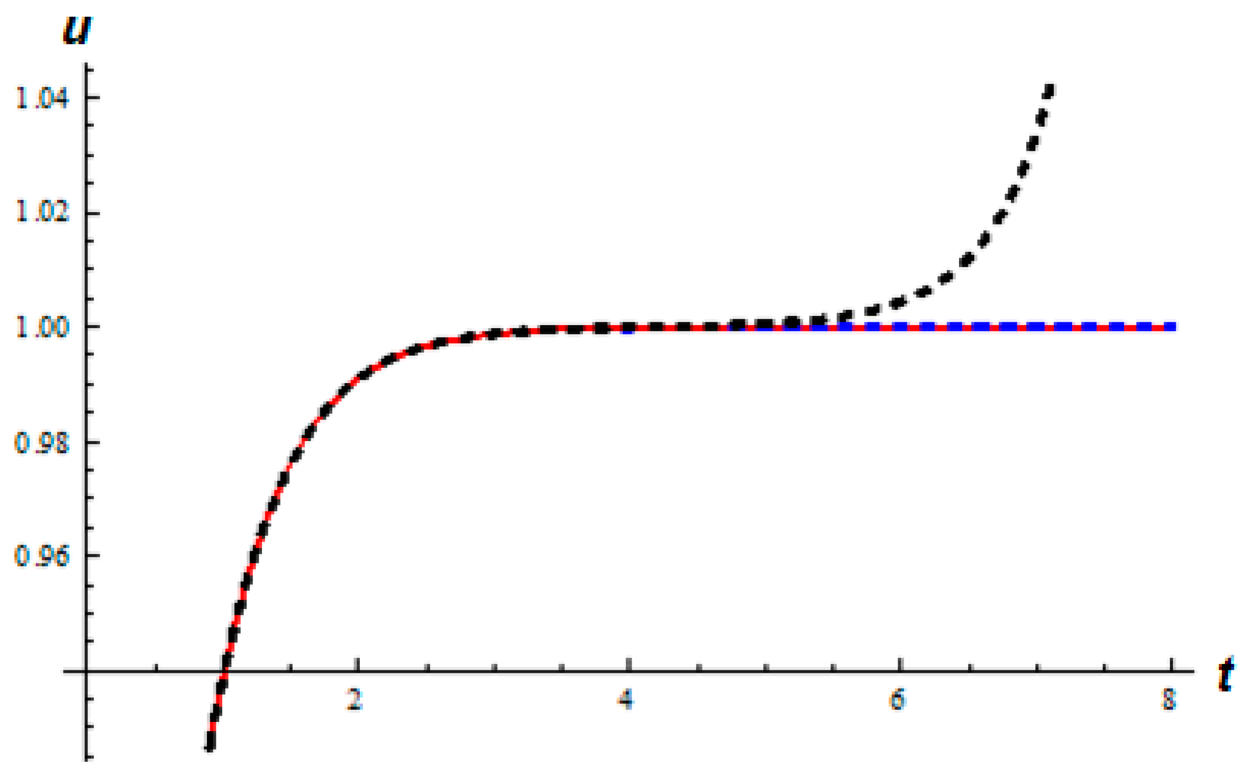
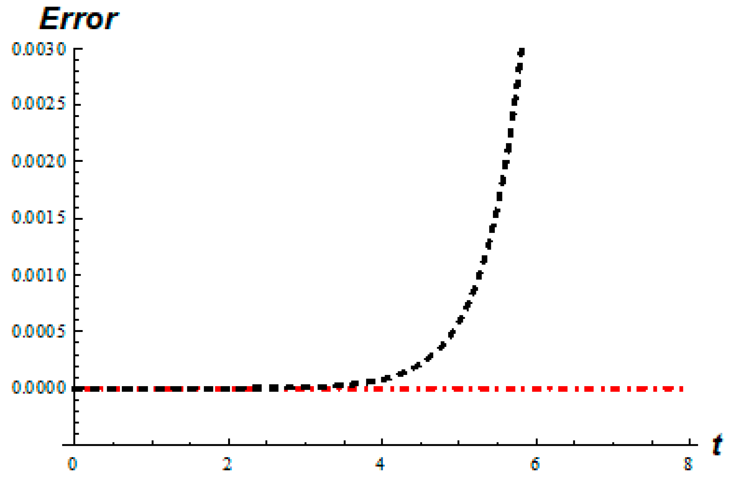
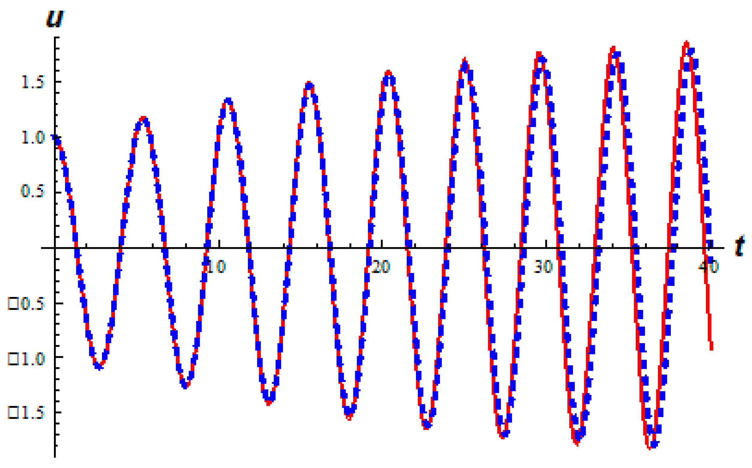
Completing solutions for our problem requires repeating this step for $i=2,3,4,\dots ,N-1$. In order to exhibit the efficiency of the presented modification with respect to RK4 method, let $\ell =-1$, $\mu =4$ and $\upsilon =-3$. Figure 1 shows the comparison of the exact solution and the 10th order multi-rule approximate analytic solution. It is obvious that our technique is very efficient and accurate, compared to RK4 method used in solving this problem. Furthermore, the domain can be expanded with a preservation of the convergence, unlike with others. The obtained absolute errors are shown in Figure 2.

Example 2. 

Consider the van der Pol oscillator in the standard form [45]

$$w^{″}-\epsilon \left(1-w^2\right)w^{\prime }+w=0,\epsilon >0,$$

(23)

which describes a position $w\left(t\right)$ of a particular as function of time $t$ with a nonlinear damping term represented by the scalar $\epsilon$. The simple harmonic motion equation is the special case when $\epsilon =0$. It is a non-conservative oscillator with linear spring force and nonlinear damping force, for which energy is degenerated at high amplitudes and generated at low amplitudes. As a consequence, there exist oscillations around a state at which energy generation and degeneracy balance out, and gives rise to a periodic motion known as a limit cycle.

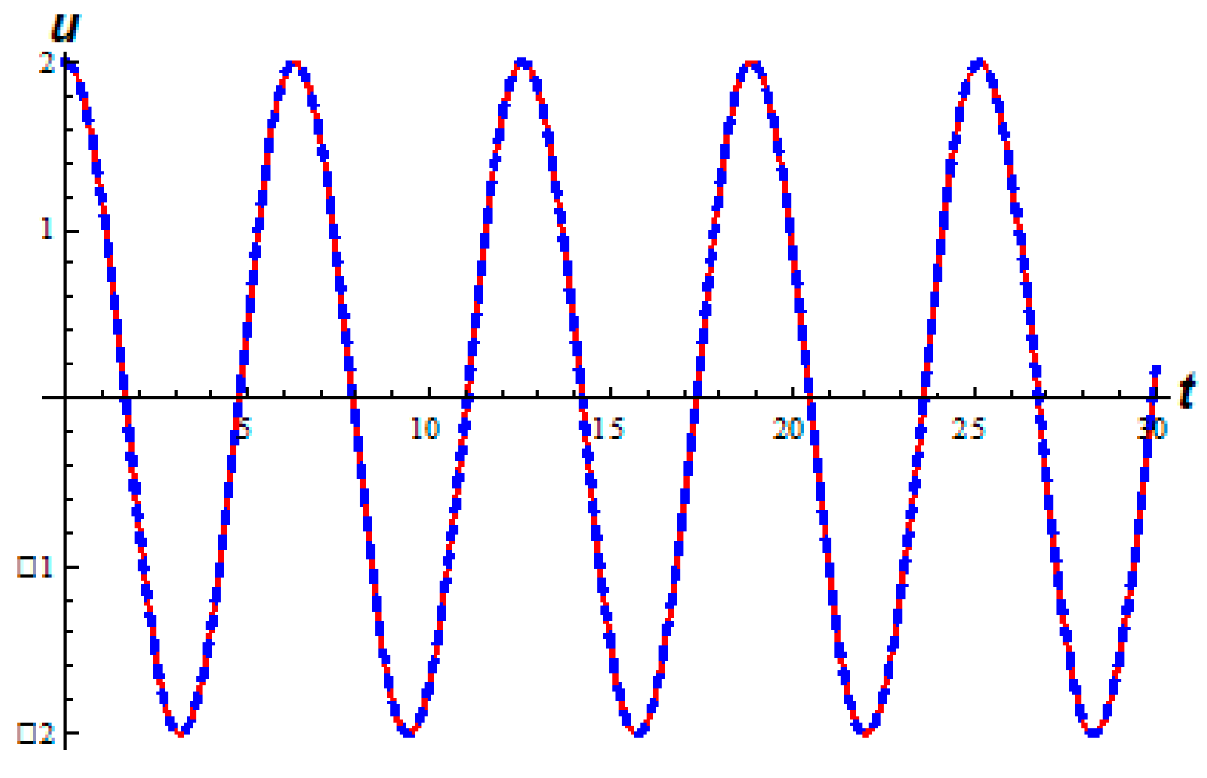
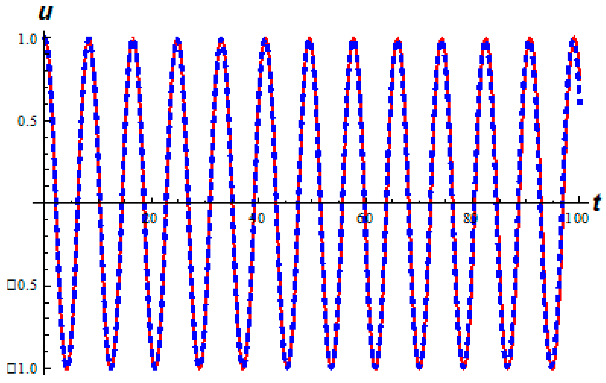
Recently, different attempts have been directed toward numeric-analytic solutions for the van der Pol oscillator, see [46] and the references therein. In order to demonstrate the advantage of our modification over the RK4 method, the behavior of 10th-order approximate displacement, with the same order approximation in the RK4 method, subject to initial data

$$w\left(0\right)=2,w^{\prime }\left(0\right)=0,$$

(24)

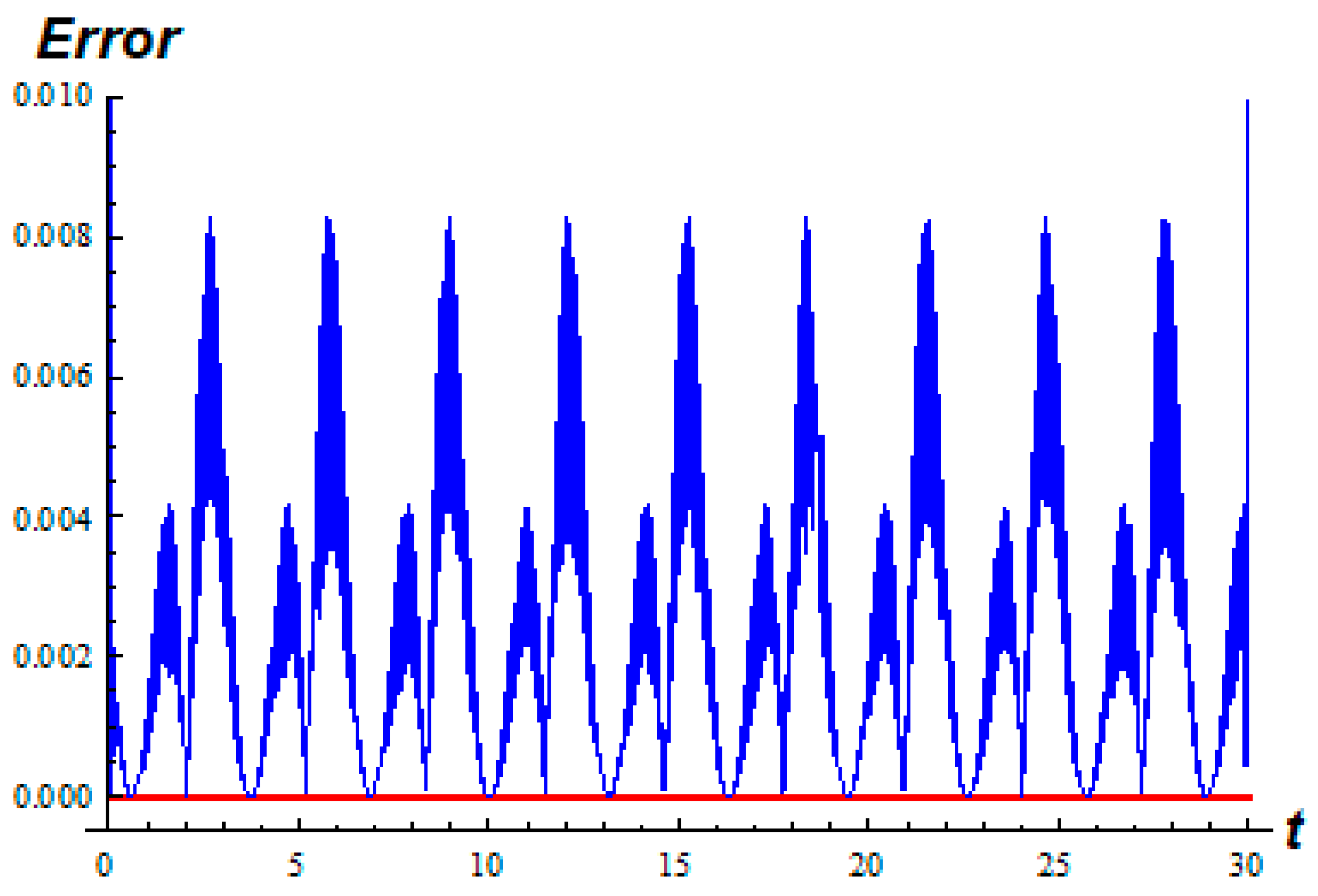
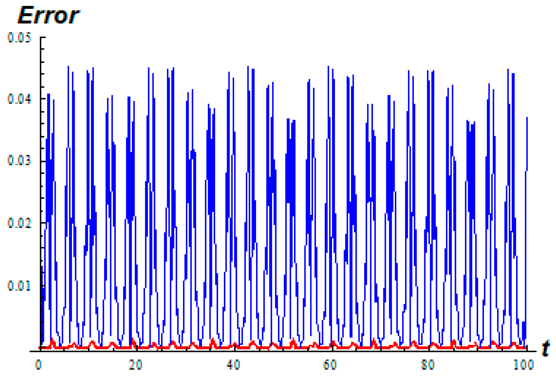
are illustrated in Figure 3. The corresponding absolute errors given in Equation (16), despite an exact solution being unknown, are shown in Figure 4. The obtained absolute errors in the case of our approximation show that the results are highly accurate that make the obtained approximate solution acceptable as a criterion of comparison.

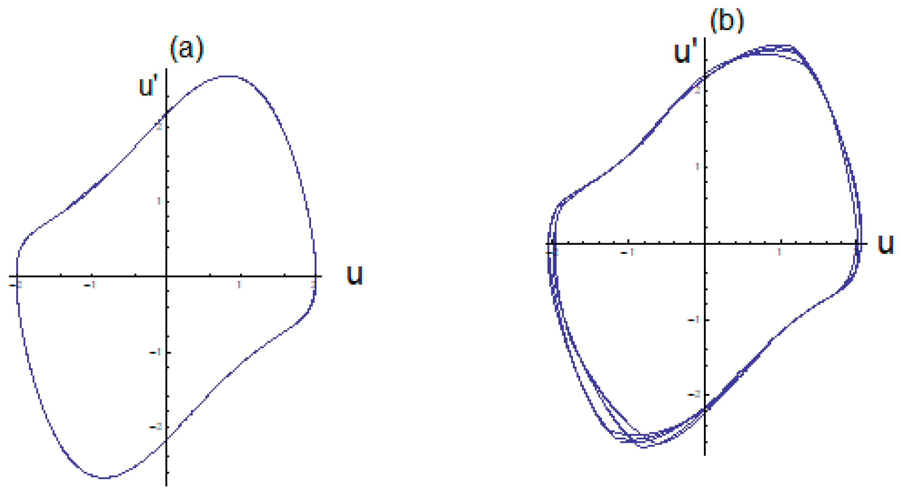
In this problem, the displacement behavior is periodic and approaches, versus velocity, the limit cycle in the phase plane. Figure 5 represents the phase plane diagrams for van der Pol oscillator at $\epsilon =1$ and the step-sizes $h=0.1$ and $h=0.5$.

Example 3. 

The classical Duffing-van der Pol oscillator is governed by the Lienard-type differential equation

$$w^{″}-\epsilon \left(1-w^2\right)w^{\prime }+\ell w+\mu w^3=0,w\left(0\right)=\alpha ,w^{\prime }\left(0\right)=\beta ,$$

(25)

where $\epsilon$, $\ell$ and $\mu$ are positive coefficients. Equation (25) has been extensively studied as an autonomous equation that describes the propagation of voltage pulses along a neural axon, in addition to potential applications in many other scientific fields, see [47] and the references therein.

Our approach constructs an analytic solution and estimates errors for several values of parameters on a large domain. As in the previous examples, the obtained results using the 10th-order solution compared to those of the RK4 method are plotted in Figure 6. Figure 7 shows the corresponding multi-rule absolute errors defined in Equation (16) with step size $h=0.5$, $\epsilon =0.1$, $\ell =1$, $\mu =0.4$, $\alpha =1$ and $\beta =0$. The modified decomposition scheme is a very powerful tool for treating the Duffing-van der Pol oscillator with a sufficiently large step-size compared to RK4 method.

Example 4. 

Consider the Lienard-type equation with rational nonlinearity

$$w^{″}+\frac{w}{1+\epsilon w^2}=0,\epsilon >0$$

(26)

subject to

$$w\left(0\right)=1,w^{\prime }\left(0\right)=0.$$

(27)

For the case of $\epsilon =1$ and the step-size $h=0.5$, the 10th-order approximate analytic solution using the modified decomposition and RK4 methods are obtained, using Mathematica [45], and graphed in Figure 8. With an unknown exact solution, the absolute errors between the two methods favoring the MDM approach, as shown in Figure 9.

5. Discussions and Conclusions

In this paper, the non-linear second order Lienard-type equation, with different nonlinearities, is considered via the multi-stage modified decomposition method. The method does not need linearization, weak nonlinearity or perturbation. It is based on combining the power series method and Adomian decomposition method by replacing nonlinearities with the corresponding Adomian polynomials expansions. While, in contrast to the Adomian decomposition method and incomputable integrals for much nonlinearity, a higher of series solution can be obtained easily using our modification. On the other hand, our technique overcomes the weakness and high complexity of power series method in solving such problems. With scientific and engineering interests, the presented technique is investigated and modified to approximate the solutions of the van der Pol and Duffing-van der Pol equations analytically. We define a continuous analytic multi-rule solution on a large interval. The errors estimation with unknown exact solutions is also obtained.

In addition to the possibility of finding exact solutions, the applicability of our modification is confirmed by the high accuracy obtained in comparison to other existing methods. The highly accurate solutions make the obtained approximations acceptable as a criterion of comparison in coming works. The stability and existence of periodic solutions (limit cycles) is included numerically.

References

- Liénard, A. Étude des oscillations entretenues. Revue Générale L’Electricité 1928, 23, 901–912. [Google Scholar]
- Salasnich, L. On the limit cycle of an inflationary universe. Nuovo Cimento B 1997, 112, 873–880. [Google Scholar]
- Écalle, J. Introduction to Analyzable Functions and Constructive Proof of the Dulac Conjecture; Hermann: Paris, France, 1992. [Google Scholar]
- Ilyashenko, S.Y. Finiteness Theorems for Limit Cycles. Translations of Mathematical Monographs; American Mathematical Society: Providence, RI, USA, 1991; p. 94. [Google Scholar]
- Zhang, Z.; Ding, T.; Huang, W.; Dong, Z. Qualitative Theory of Differential Equations, Translations of Mathematical Monographs; American Mathematical Society: Providence, RI, USA, 1992; p. 101. [Google Scholar]
- Lefschetz, S. Existence of periodic solutions for certain differential equations. Proc. Natl. Acad. Sci. USA 1943, 29, 29–32. [Google Scholar] [CrossRef]
- Cesari, L. Asymptotic Behaviour and Stability Problems in Ordinary Differential Equations; Springer: Berlin, Germany, 1963. [Google Scholar]
- Graef, J. On the generalized Liénard equation with negative damping. J. Differ. Equ. 1972, 12, 34–62. [Google Scholar] [CrossRef]
- Zhang, L.-H.; Wang, Y. A note on periodic solutions of a forced Linard-type equation. ANZIAM J. 2010, 51, 350–368. [Google Scholar] [CrossRef]
- Nayfeh, A.H.; Mook, D.T. Nonlinear Oscillations; John Wiley: New York, NY, USA, 1979. [Google Scholar]
- Xu, L. He’s parameter-expanding methods for strongly nonlinear oscillators. J. Comput. Appl. Math. 2007, 207, 148–154. [Google Scholar] [CrossRef]
- Batiha, K.; Batiha, B. The variational iteration method for solving nonlinear oscillator. Appl. Math. Sci. 2012, 6, 1771–1777. [Google Scholar]
- Az-Zo’bi, E.A. On the convergence of variational iteration method for solving systems of conservation laws. Trends Appl. Sci. Res. 2015, 10, 157–165. [Google Scholar]
- He, J.H. The homotopy perturbation method for nonlinear oscillators with discontinuities. Appl. Math. Comput. 2004, 151, 287–292. [Google Scholar] [CrossRef]
- Az-Zo’bi, E.A.; Al Dawoud, K.; Marashdeh, M. Numeric-analytic solutions of mixed-type systems of balance laws. Appl. Math. Comput. 2015, 265, 133–143. [Google Scholar] [CrossRef]
- Matinfar, M.; Bahar, S.R.; Ghasemi, M. Solving the Lienard equation by differential transform method. World J. Model. Simul. 2012, 8, 142–146. [Google Scholar]
- Az-Zo’bi, E.A. On the reduced differential transform method and its application to the generalized Burgers-Huxley equation. Appl. Math. Sci. 2014, 8, 8823–8831. [Google Scholar] [CrossRef]
- Ghosh, S.; Roy, A.; Roy, D. An adaptation of Adomian decomposition for numeric-analytic integration of strongly nonlinear and chaotic oscillators. Comput. Methods Appl. Mech. Eng. 2007, 196, 1133–1153. [Google Scholar] [CrossRef]
- Az-Zo’bi, E.A. Modified Laplace decomposition method. World Appl. Sci. J. 2012, 18, 1481–1486. [Google Scholar]
- Az-Zo’bi, E.A. An approximate analytic solution for isentropic flow by an inviscid gas equations. Arch. Mech. 2014, 66, 203–212. [Google Scholar]
- Az-Zo’bi, E.A. New applications of Adomian decomposition method. Middle-East J. Sci. Res. 2015, 23, 735–740. [Google Scholar]
- Syam, M.I. A numerical solution of fractional Lienard’s equation by using the residual power series method. Mathematics 2018, 6, 1. [Google Scholar] [CrossRef]
- Az-Zo’bi, E.A. Analytic simulation for 1D Euler-like model in fluid dynamics. J. Adv. Phys. 2018, 7, 330–335. [Google Scholar] [CrossRef]
- Az-Zo’bi, E.A. Exact analytic solutions for nonlinear diffusion equations via generalized residual power series method. Int. J. Math. Comput. Sci. 2019, 14, 69–78. [Google Scholar]
- Az-Zo’bi, E.A.; Yıldırım, A.; AlZoubi, W.A. The residual power series method for the one-dimensional unsteady flow of a van der Waals gas. Physica A 2019, 517, 188–196. [Google Scholar] [CrossRef]
- Adomian, G.; Rach, R. Transformation of series. Appl. Math. Lett. 1991, 4, 69–71. [Google Scholar] [CrossRef] [Green Version]
- Adomian, G.; Rach, R. Nonlinear transformation of series—Part II. Comput. Math. Appl. 1992, 23, 79–83. [Google Scholar] [CrossRef]
- Az-Zo’bi, E.A.; Maysoon Qousini, M. Modified Adomian-Rach decomposition method for solving nonlinear time-dependent IVPs. Appl. Math. Sci. 2017, 11, 387–395. [Google Scholar] [CrossRef]
- Duan, J.-S.; Rach, R.; Wazwaz, A.-M. Higher order numeric solutions of the Lane-Emden-type equations derived from the multi-stage modified Adomian decomposition method. Int. J. Comput. Math. 2017, 94, 197–215. [Google Scholar] [CrossRef]
- Adomian, G.; Rach, R. Inversion of nonlinear stochastic operators. J. Math. Anal. Appl. 1983, 91, 39–46. [Google Scholar] [CrossRef] [Green Version]
- EL-Kalla, I.L.; El Mhlawy, A.M.; Botros, M. A continuous solution of solving a class of nonlinear two point boundary value problem using Adomian decomposition method. Ain Shams Eng. J. 2019, 10, 211–216. [Google Scholar] [CrossRef]
- Az-Zo’bi, E.A.; Al Khaled, K. A new convergence proof of the Adomian decomposition method for a mixed hyperbolic elliptic system of conservation laws. Appl. Math. Comput. 2010, 217, 4248–4256. [Google Scholar] [CrossRef]
- Az-Zo’bi, E.A. Construction of solutions for mixed hyperbolic elliptic Riemann initial value system of conservation laws. Appl. Math. Model. 2013, 37, 6018–6024. [Google Scholar] [CrossRef]
- Wazwaz, A.-M.; Rach, R.; Duan, J.-S. Steady-state concentrations of carbon dioxide absorbed into phenyl glycidal ether solutions by the Adomian decomposition method. J. Math. Chem. 2015, 53, 1054–1067. [Google Scholar]
- Rach, R.; Duan, J.-S.; Wazwaz, A.-M. Solution of higher-order, multipoint, nonlinear boundary value problems with higher-order Robin-type boundary conditions by the Adomian decomposition method. Appl. Math. Inf. Sci. 2016, 10, 1231–1242. [Google Scholar] [CrossRef]
- Cherruault, Y. Convergence of Adomian’s method. Kybernetes 1989, 18, 31–38. [Google Scholar] [CrossRef]
- Abbaoui, K.; Cherruault, Y. Convergence of Adomian’s method applied to nonlinear equations. Math. Comput. Model. 1994, 20, 60–73. [Google Scholar] [CrossRef]
- Rèpaci, A. Nonlinear dynamical systems: On the accuracy of Adomian’s decomposition method. Appl. Math. Lett. 1990, 3, 35–39. [Google Scholar] [CrossRef]
- Rach, R.; Adomian, G.; Meyers, R.E. A modified decomposition. Comput. Math. Appl. 1992, 23, 17–23. [Google Scholar] [CrossRef] [Green Version]
- Feng, Z. On explicit exact solutions for the Lienard equation and its applications. Phys. Lett. A 2002, 293, 50–56. [Google Scholar] [CrossRef]
- Kaya, D.; El-Sayed, S.M. A numerical implementation of the decomposition method for the Lienard equation. Appl. Math. Comput. 2005, 171, 1095–1103. [Google Scholar] [CrossRef]
- Matinfar, M.; Mahdavi, M.; Raeisy, Z. Exact and numerical solution of Lienard’s equation by the variational homotopy perturbation method. J. Inf. Comput. Sci. 2011, 6, 73–80. [Google Scholar]
- Heydari, M.H.; Hooshmandasl, M.R.; Maalek Ghain, F.M. A good approximate solution for lienard equation in a large interval using block pulse functions. J. Math. Ext. 2013, 7, 17–32. [Google Scholar]
- Wolfram Research, Inc. Mathematica, Version 9.0; Wolfram Research, Inc.: Champaign, IL, USA, 2012. [Google Scholar]
- Van der Pol, B. On relaxation-oscillations. Lond. Edinb. Dublin Philos. Mag. J. Sci. 1927, 2, 978–992. [Google Scholar] [CrossRef]
- Ramana, P.V.; Raghu Prasad, B.K. Modified Adomian decomposition method for Van der Pol equations. Int. J. Non-Linear Mech. 2014, 65, 121–132. [Google Scholar] [CrossRef]
- Kyzioł, J.; Okniński, A. The Duffing–Van der Pol equation: metamorphoses of resonance curves. Nonlinear Dyn. Syst. Theory 2015, 15, 25–31. [Google Scholar]
Figure 1.
Plots of the exact solution (blue dashed line, see Equation (20)) versus approximate analytic solution (red solid line, see Equation (21) for n = 10) and RK4 method (black dashed line) using the MDM for and .
Figure 2.
The absolute errors corresponding to approximate solutions using the MDM (red dash-dotted line) and RK4 method (black dashed line) for and .
Figure 3.
Plots of approximate displacement (red solid line) using the MDM and RK4 method (blue dashed line) for and step-size .
Figure 4.
The absolute errors corresponding to approximate solutions using the MDM (red solid line) and RK4 method (blue line) for and step-size .
Figure 5.
The limit cycles of van der Pol oscillator for and the step-size (a) , (b) on the interval .
Figure 6.
Plots of approximate solution (see Equation (15) using the modified decomposition method (red solid line) and RK4 method (blue dashed line) for and step-size .
Figure 7.
The corresponding absolute errors to approximate solutions using the modified decomposition method (red solid line) and RK4 method (blue line) for and step-size .
Figure 8.
Plots of approximate solution using the MDM (red solid line) and RK4 method (blue dashed line) for and step-size .
Figure 9.
The corresponding absolute errors to approximate solutions using the MDM (red solid line) and RK4 method (blue line) for and step-size .
© 2019 by the authors. Licensee MDPI, Basel, Switzerland. This article is an open access article distributed under the terms and conditions of the Creative Commons Attribution (CC BY) license (http://creativecommons.org/licenses/by/4.0/).
Share and Cite
MDPI and ACS Style
Az-Zo’bi, E.A.; Al-Khaled, K.; Darweesh, A. Numeric-Analytic Solutions for Nonlinear Oscillators via the Modified Multi-Stage Decomposition Method. Mathematics 2019, 7, 550. https://0-doi-org.brum.beds.ac.uk/10.3390/math7060550
AMA Style
Az-Zo’bi EA, Al-Khaled K, Darweesh A. Numeric-Analytic Solutions for Nonlinear Oscillators via the Modified Multi-Stage Decomposition Method. Mathematics. 2019; 7(6):550. https://0-doi-org.brum.beds.ac.uk/10.3390/math7060550
Chicago/Turabian StyleAz-Zo’bi, Emad A., Kamel Al-Khaled, and Amer Darweesh. 2019. "Numeric-Analytic Solutions for Nonlinear Oscillators via the Modified Multi-Stage Decomposition Method" Mathematics 7, no. 6: 550. https://0-doi-org.brum.beds.ac.uk/10.3390/math7060550
Note that from the first issue of 2016, this journal uses article numbers instead of page numbers. See further details here.