Restricted Gompertz-Type Diffusion Processes with Periodic Regulation Functions


Dipartimento di Informatica, Università degli Studi di Salerno, Via Giovanni Paolo II n. 132, 84084 Fisciano (SA), Italy
*
Author to whom correspondence should be addressed.
†
These authors contributed equally to this work.
Mathematics 2019, 7(6), 555; https://0-doi-org.brum.beds.ac.uk/10.3390/math7060555
Submission received: 6 June 2019
/
Revised: 14 June 2019
/
Accepted: 14 June 2019
/
Published: 18 June 2019
(This article belongs to the Special Issue Diffusion Processes Associated with Growth Curves: Probabilistic and Inferential Analysis)
Abstract
:We consider two different time-inhomogeneous diffusion processes useful to model the evolution of a population in a random environment. The first is a Gompertz-type diffusion process with time-dependent growth intensity, carrying capacity and noise intensity, whose conditional median coincides with the deterministic solution. The second is a shifted-restricted Gompertz-type diffusion process with a reflecting condition in zero state and with time-dependent regulation functions. For both processes, we analyze the transient and the asymptotic behavior of the transition probability density functions and their conditional moments. Particular attention is dedicated to the first-passage time, by deriving some closed form for its density through special boundaries. Finally, special cases of periodic regulation functions are discussed.
MSC:
60J60; 60K37; 60J70; 92D251. Introduction
Deterministic and stochastic growth models are been widely used in the literature to study dynamics of a population. Some such models, as the logistic and Gompertz ones, are characterized by an intrinsic rate of growth and by a horizontal asymptote; both can be time-dependent. This limit, called carrying capacity function, can be caused by many environmental factors as living space, food availability and water supply. In particular, Coleman et al. [1] analyzes the behavior of the deterministic logistic model in the periodic environment by assuming that the intrinsic growth coefficient and the carrying capacity are periodic time-dependent function. In Mir [2] and in Mir and Dubeau [3], the authors study the effect of different time-dependent carrying capacities in deterministic Richards models, including logistic and Gompertz growths. Tjørve and Tjørve [4,5] propose a unified approach to the Richards-model family to describe the growth of animals and plants, as well as the number of bacteria and the volume of cancer cells.
The deterministic approach presents some limitations in mathematical biology since it is always arduous to predict the evolution of the system accurately. Indeed, the biological systems are subject to random fluctuations, due partially to environment factors, such as epidemics and nature disasters. To take into account the environmental fluctuations, often responsible for the discrepancies between experimental data and theoretical predictions, the idea of growth in random environment has been considered by various authors (cf., for instance, Goel and Richter-Dyn [6], Ricciardi [7,8] and Ricciardi et al. [9]). Some diffusion growth models in random environment are considered in Capocelli and Ricciardi [10], Tuckwell [11], Nobile and Ricciardi [12,13], Skiadas [14], and Kink [15]. Analytical properties of logistic and other growth models are taken into account in Di Crescenzo and Spina [16] and Di Crescenzo and Paraggio [17].
The Gompertz model is widely used in many aspects of biology because it can fit well the experimental date related to the evolution of same populations of organisms and of certain solid tumors (cf., for instance, [5] and references therein). In the classical Gompertz model, the intrinsic growth coefficient and the carrying capacity are chosen as constant parameters. However, sometimes the description of certain phenomena requires the use of time-dependent functions; in these cases, the Gompertz model turns out to be particularly effective to describe the population dynamics. For this reason, many efforts have recently been made to investigate the analytical and statistical properties of time-inhomogeneous Gompertz models. Specifically, the studies have focused on the following topics: (i) analysis of probabilistic characteristics, as the transition probability densities, the first-passage time density through a particular time dependent threshold (cf. Albano et al. [18,19], Ghost and Prajneshu [20]); (ii) discovery of appropriate procedures to estimate the unknown parameters and the time dependent functions characterizing the infinitesimal moments of the diffusion process (see, Gutiérrez et al. [21], Moummou et al. [22,23], Albano et al. [24,25], Román-Román et al. [26]); (iii) study of stochastic Gompertz process with jumps that occur at random time and reset the process to a fixed value; after each jump, the process restarts with modified grows parameters (see Spina et al. [27], Giorno et al. [28]). The Gompertz growth model plays a special role also in nonlinear models of interacting populations (cf., for instance, Goel et al. [29]) and in a non-autonomous predator–prey system (cf. Buonocore et al. [30]).
In the present paper, we consider two different time-inhomogeneous diffusion processes useful to model the evolution of a population in a random environment. They are obtained as approximations of the solution of deterministic Gompertz-type growth models. The first considered process is an unrestricted time-inhomogeneous Gompertz diffusion process, whereas the second one is a restricted diffusion process, obtained by including a reflecting condition. Indeed, sometimes in growth models, the population is not isolated, so that immigration effects may be occur. In these cases, it is necessary take into account diffusion processes with a reflecting condition in the zero state. A special diffusion process in the presence of reflecting boundaries are taken into account in Linetsky [31], Giorno et al. [32,33], and Buonocore et al. [34,35].
In Section 2, we consider the Gompertz diffusion process with growth rate , carrying capacity and noise intensity , whose conditional median coincides with the deterministic Gompertz growth. Results concerning the transition probability density function (pdf) and its moments are derived. Particular attention is dedicated to analyzing the first-passage time (FPT) problem and the asymptotic behavior of the transition densities and of the FPT densities through a constant boundary S in two cases: (a) for asymptotically constant functions and for (b) for asymptotically constant functions with periodic function. In Section 3, we assume that the carrying capacity is a periodic time-dependent function and specialize the results of Section 2 when and ; same comparisons are carried out for (i) and for (ii) in order to highlight both the role of .
In Section 4, we perform a similar analysis for the Gompertz process in the presence of a reflecting boundary in zero state. Since, in the Gompertz process considered in Section 2 and Section 3 the state zero is unattainable, in Section 4, we build the restricted process by shifting the original Gompertz process and then by introducing in this last one a reflecting condition in the zero state. For the restricted process , the function represents again the growth rate, is a regulation function and gives the noise intensity. For this process, we analyze the transient and asymptotic behavior of the transition pdf and of FPT density through the constant boundary. Finally, in Section 5, the process is studied for the same cases of Section 3 with and in order to highlight both the role of and the effect of the reflecting condition on the population growth.
2. Time-Inhomogeneous Gompertz-Type Growth
In this section, we analyze the inhomogeneous deterministic and stochastic Gompertz model. For the stochastic process, we focus on the transition pdf and its moments, on the FPT density and on the asymptotic behavior of the process.
2.1. Deterministic Evolution
Let and be continuous functions. We assume that the population density evolves according to the Gompertz law:
where and
The function represents the growth rate of the population and the function describes the time-dependent carrying capacity. Indeed, if then for all , whereas, if then for all .
We remark that Label (1) is solution of the differential equation:
From (1), the population density at time can be expressed as:
Starting from (3), a time-inhomogeneous stochastic diffusion process can be constructed.
2.2. Stochastic Evolution
Under the assumption of random environment, we interpret as the mean of the increment of a time-inhomogeneous Wiener process having mean function and covariance function , where is a continuous function. Therefore,
where is the standard Wiener process.
Making use of the assumption of random environment, denoting by the stochastic process describing the evolution of the population, from (3), one obtains the following stochastic equation:
from which one derives:
From (7), we note that is a time-inhomogeneous Gompertz-type diffusion process with space-state having infinitesimal drift and variance and , respectively. We remark that the boundaries 0 and are unattainable states for . The transition pdf of is solution of the Fokker–Planck equation with the initial delta condition:
Therefore, is the transition pdf of a time-inhomogeneous Ornstein–Uhlenbeck process with state-space , whose infinitesimal drift and variance are given in (11). Hence, is a normal pdf with conditional mean and variance:
respectively. Recalling (9), the transition pdf of is lognormal:
Moreover, conditional mean, median and variance are:
We note that the conditional median of does not dependent upon and it coincides with the deterministic solution given in (1). Furthermore, when is zero, the conditional mean is identified with the deterministic solution and the conditional variance is zero.
2.3. First-Passage Time Problem for
We consider the FPT problem for the diffusion process with infinitesimal moments (7). Let
be the random variable that describes the FPT of from to the continuous boundary . The FPT pdf is solution of the first-kind Volterra integral equation:
Due to (9), one has , where is the FPT density of the Ornstein–Uhlenbeck process with infinitesimal moments (11). Then, making use of the results given in Di Nardo et al. [36], the FPT density is a solution of the following non-singular second-kind Volterra integral equation:
with when and when , where
2.4. Asymptotic Behavior for
We analyze the asymptotic behavior of the process when the functions and admit finite limits as the time increases by distinguishing two different cases: (a) admits a finite limit and (b) is a periodic function of period Q.
Case(a) We assume that
Under the assumptions (22), we analyze the asymptotic behavior of the FPT density through a constant boundary , with . As the threshold S is progressively moved away from the starting point of the process , an exponential approximation is shown to hold for the FPT pdf (cf. [38,39]). Indeed, if and or if and , the following behavior holds:
where
with given in (18) and when and when .
Case(b) We suppose that
Under the assumptions (28), we analyze the asymptotic behavior of the FPT density through a constant boundary , with . From (18), one has:
with when and when . Furthermore, denoting by , we have that if and or if and for all . As the threshold S moves away from , a time-inhomogeneous exponential approximation holds for the FPT pdf (cf. [38,39]). Indeed, if and or if and , for all , one has:
with given in (32).
3. A Special Gompertz-Type Growth with Periodic Carrying Capacity
In the deterministic and stochastic Gompertz-type model, we assume that the growth rate and the carrying capacity is a periodic function of period Q, such that
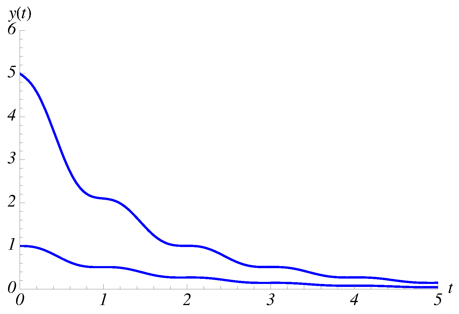
In Figure 1, we plot the deterministic curves , given in (1), for and (solid blue curves); the dashed curve represents the periodic carrying capacity .
Moreover, in the stochastic Gompertz model with infinitesimal moments (7), we consider two cases: (i) and (ii) , with .
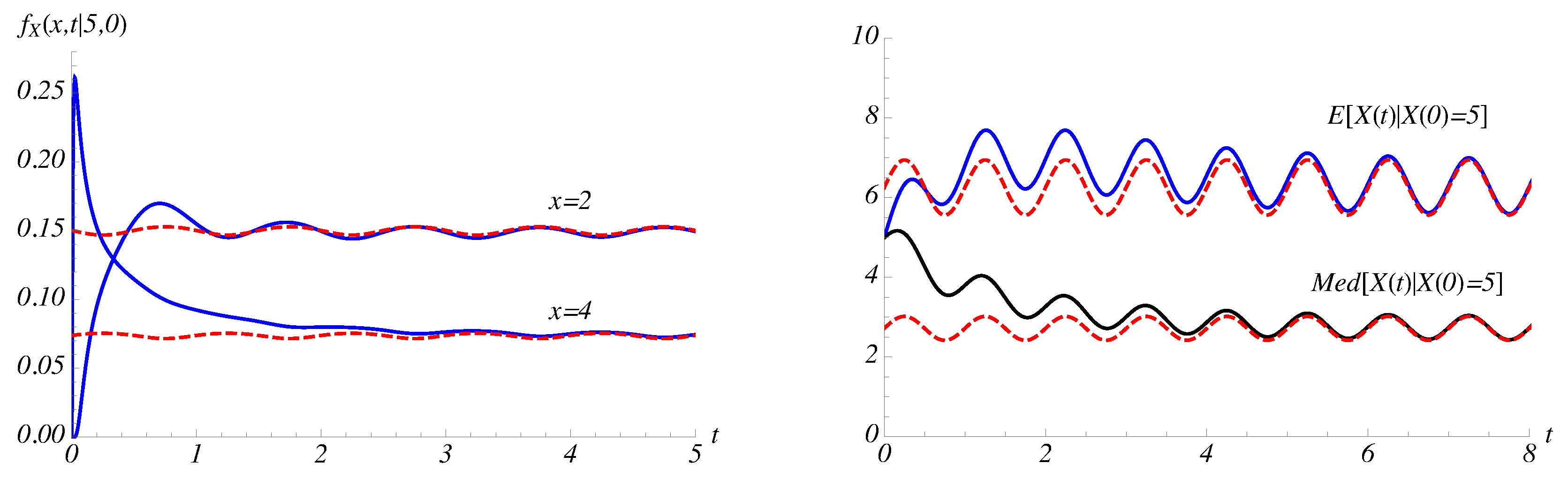
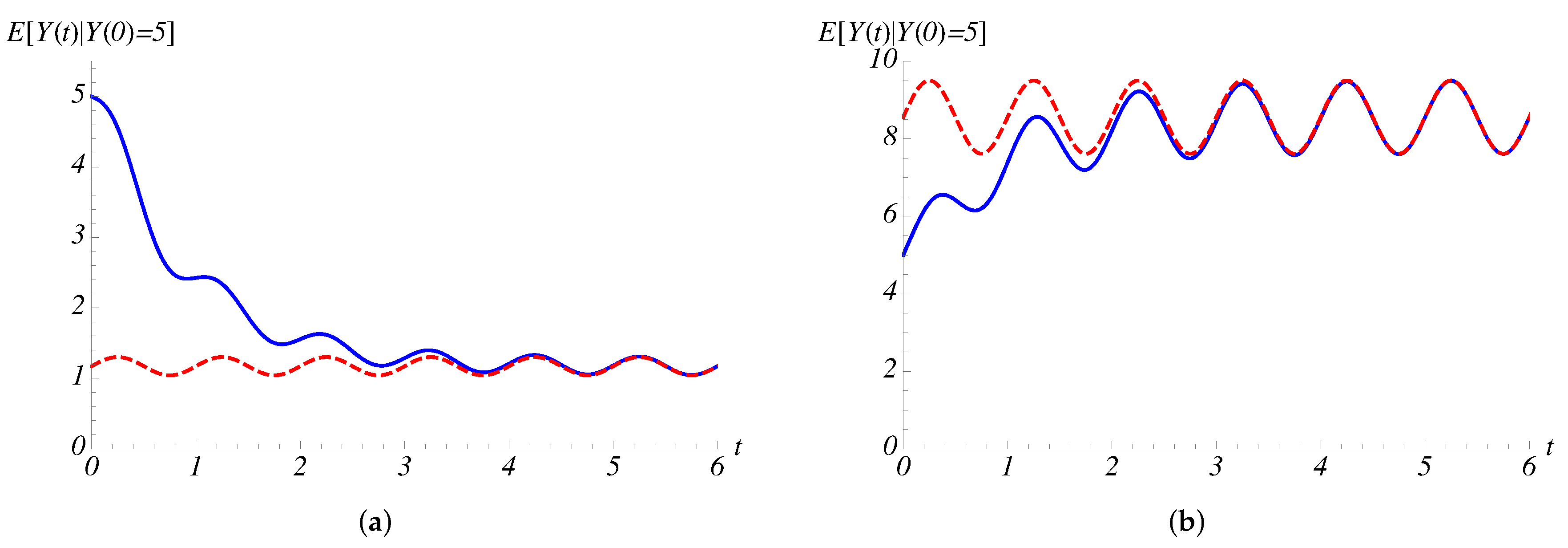
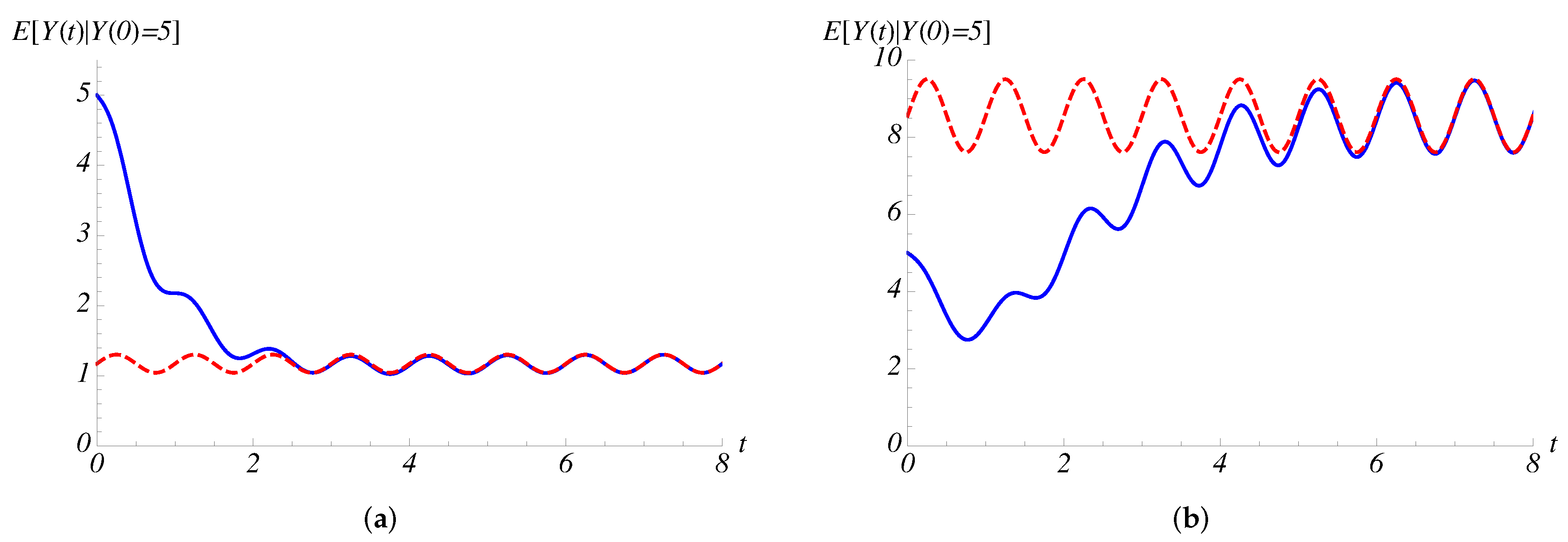
For the same choices as Figure 1, with and , on the left of Figure 2, we plot the transition pdf, given in (13), as function of t when and (solid blue curves); the dashed curves represent the corresponding asymptotic densities, obtained from (30). On the right of Figure 2, for the same choices as Figure 1 with and , the conditional mean and median (14) are compared with the corresponding asymptotic behaviors, given in (31). Note that the median coincides with the deterministic curve plotted in Figure 1.
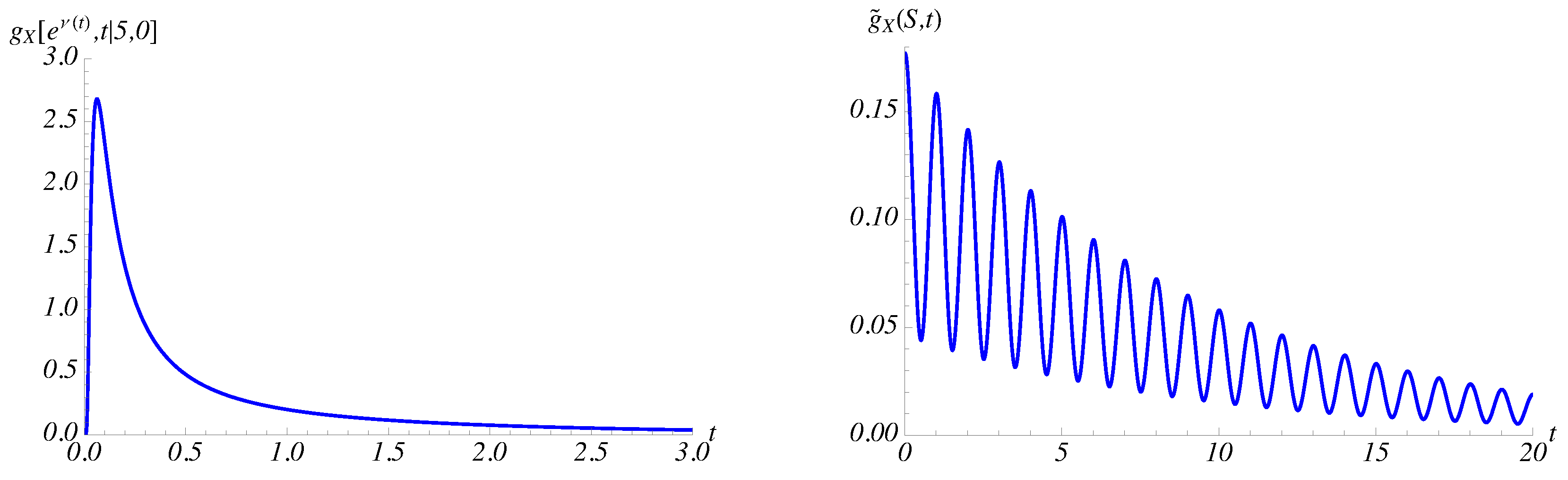
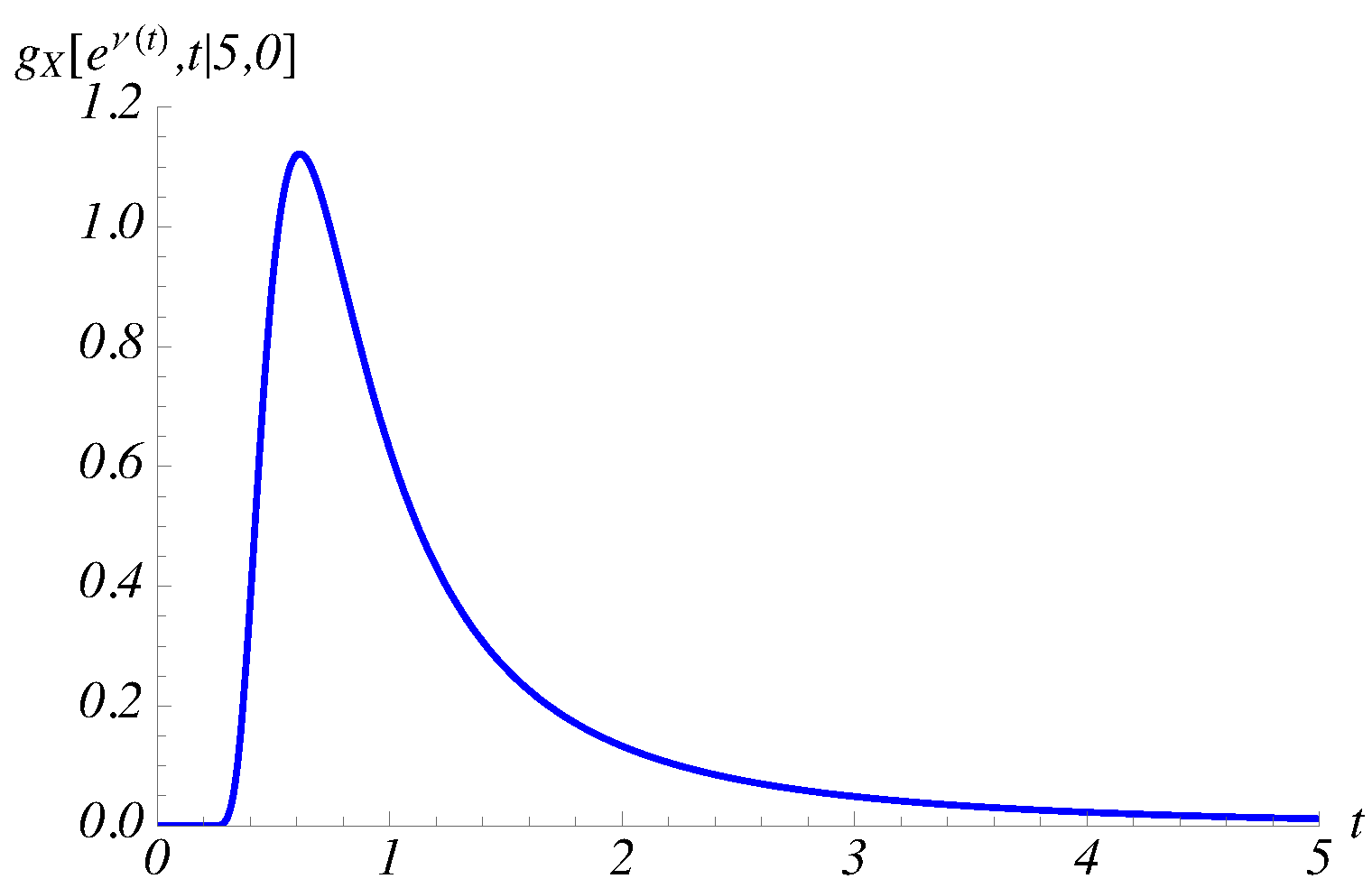
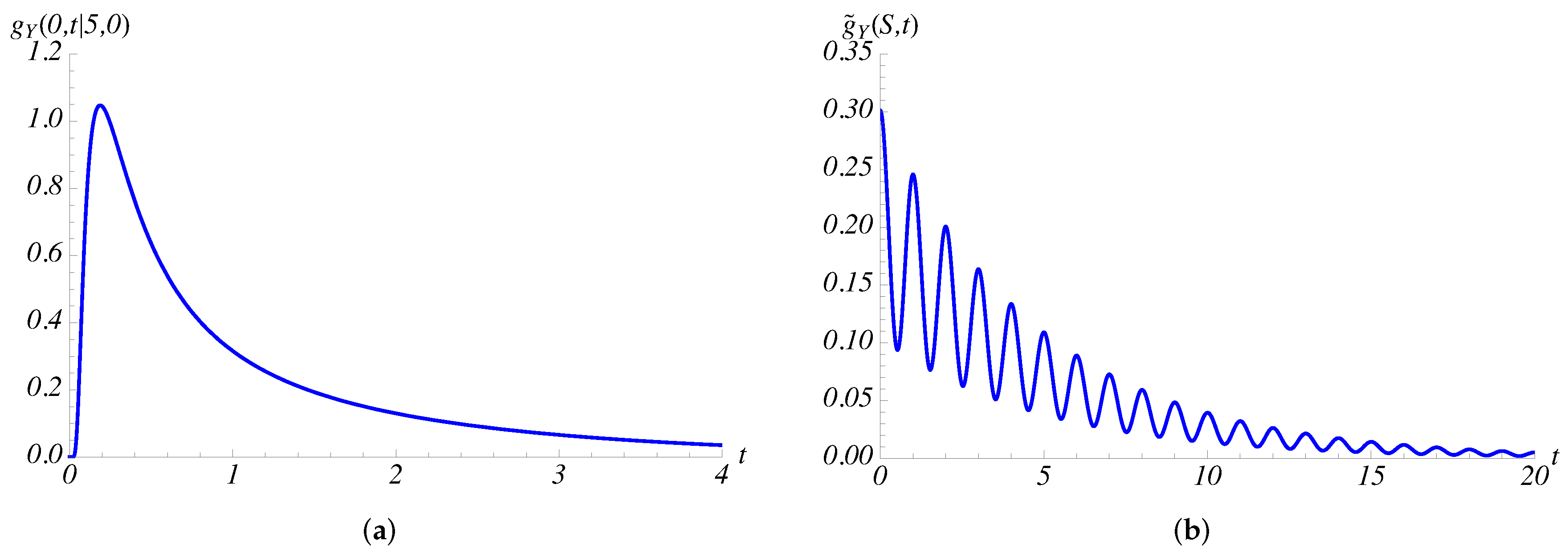
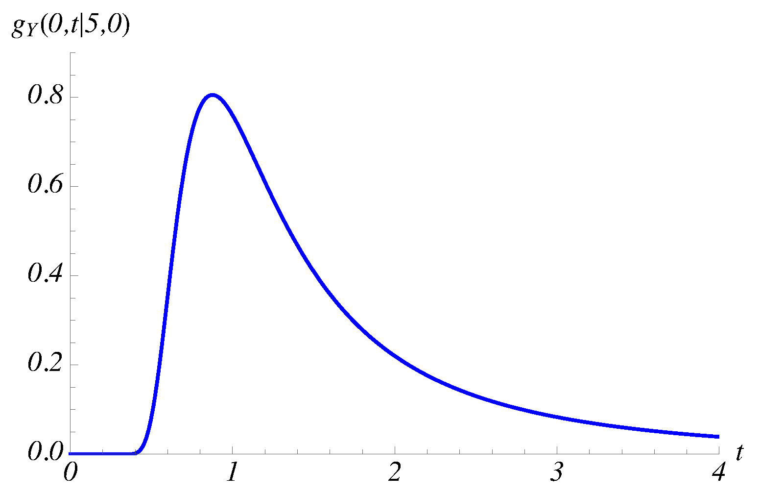
On the left of Figure 3, the FPT pdf through the carrying capacity , given in (20), is plotted as function of t for the same choices as Figure 1, with and . Note that, in this case, the shape of the FPT pdf is not affected by the periodicity of the boundary. Moreover, on the right of Figure 3, we plot the asymptotic behavior , given in (33), of the FPT density through the constant boundary when .
Case(ii) Let
where is a real positive constant. In this case, is an increasing monotonic function which tends to as . From (12), one has:
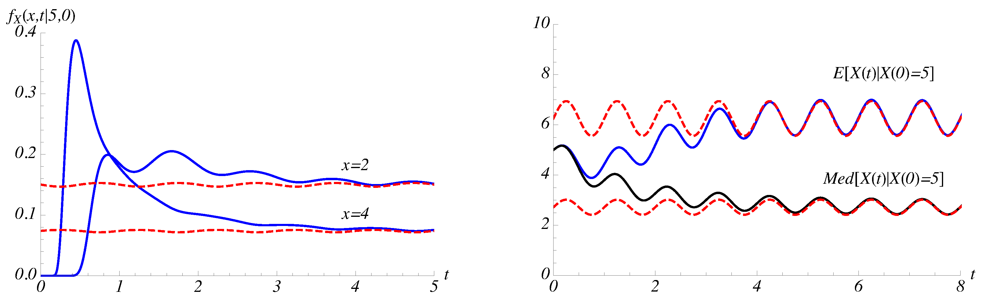
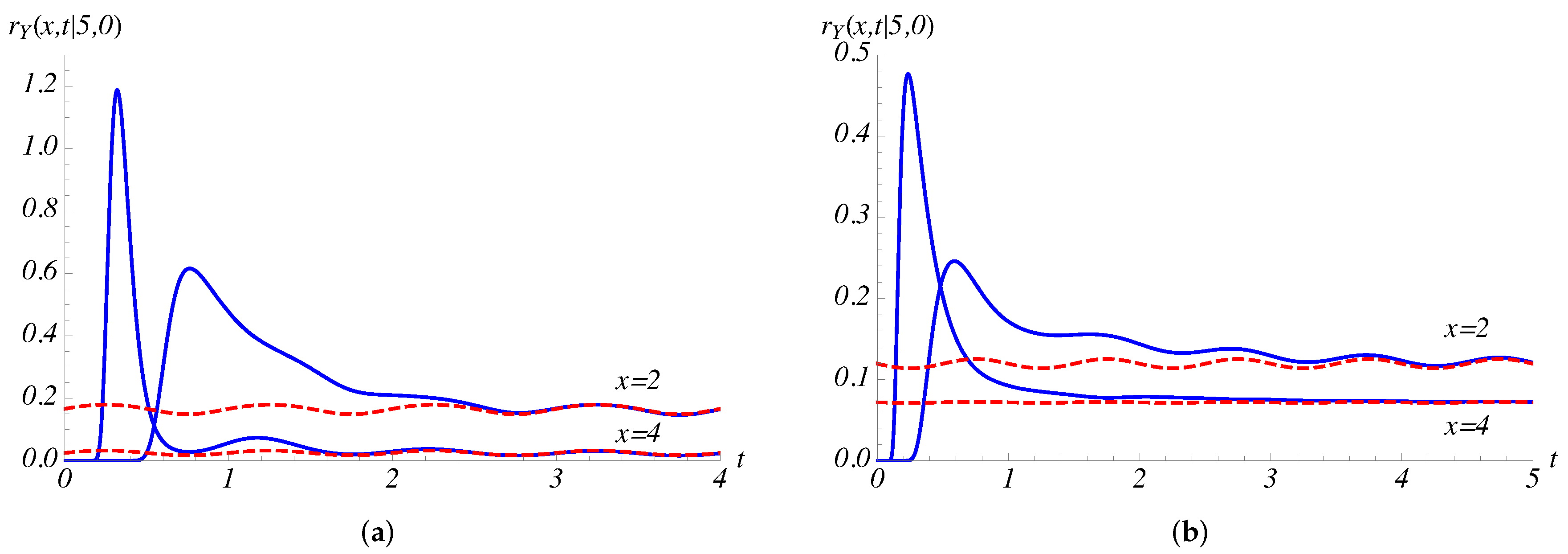
For the same choices as Figure 1, with and given in (36) with , on the left of Figure 4, we plot the transition densities, given in (13), as function of t when and (solid blue curves); the dashed curves represent the corresponding asymptotic densities, obtained from (30). On the right of Figure 4, for the same choices as Figure 1 with and , the conditional mean and median (14) are compared with the corresponding asymptotic behaviors, given in (31). Note that, also in this case, the median coincides with the deterministic curve plotted in Figure 1. By comparing Figure 2 and Figure 4, we remark that the asymptotic behaviors are the same, the medians are the same, whereas some differences are highlighted on the averages. Furthermore, the transient behaviors of the transition pdf of Figure 4 are delayed with respect to those shown in Figure 2.
4. Time-Inhomogeneous Restricted Gompertz-Type Growth
In this section, to take into account immigration effects, occurring when the population is not isolated, we analyze a Gompertz-type diffusion process restricted by a reflecting boundary in the zero state. We remark that in the classical Gompertz process the state zero is unattainable, so that, to build the restricted process, we first shift the original Gompertz process and then we introduce in this last one a reflecting condition in the zero state. For the obtained restricted diffusion process, we determine the transition pdf and its moments; furthermore, we analyze the FPT problem and we study the asymptotic behavior.
4.1. Deterministic Evolution
Starting from (1), we perform the transformation , so that evolves according to the following law:
with and given in (2). Since , one has for all and , so that the population size decreases to zero and the extinction takes place when t tends to infinity. Therefore, differently from the Gompertz-type model, analyzed in Section 2, in this case, does not represent the carrying capacity, rather it can be interpreted as a regulation function that influences the population dynamics. From (38), we have:
By using (38), the population density at time can be expressed as follows:
Starting from (39), a stochastic restricted time-inhomogeneous diffusion process can be constructed.
4.2. Stochastic Evolution
Under the same assumption of random environment of Section 2.2, starting from (39), we consider the stochastic process that satisfies the following stochastic equation:
with given in (4). Proceeding as in Section 2.2, we obtain the infinitesimal moments of :
Hence, is a time-inhomogeneous diffusion process with space-state having infinitesimal drift and variance and , respectively. The transition pdf is
with given in (13).
In order to describe the population dynamics, we consider the stochastic process , obtained by restrict the space-state of to the interval , with 0 reflecting boundary. This ensures that the population does not become extinct. The transition pdf of the restricted diffusion process is a solution of the Fokker–Planck equation and satisfies the reflecting condition in zero state and the initial delta condition:
with given in (41). The second equation in (43) expresses a zero-flux condition at for the restricted process . Making use of transformations:
from (43), one has:
with and given in (11). Therefore, is the transition pdf of a restricted time-inhomogeneous Ornstein–Uhlenbeck process restricted to the state-space by a reflecting condition in . The second equation in (45) expresses a zero-flux condition at for the restricted Ornstein–Uhlenbeck. As proved in Buonocore et al. [34], one has
where is a normal pdf with conditional mean and variance given in (12). Recalling (44), the transition pdf of is
Moreover, setting , the conditional mean and second order moment are:
where denotes the error function. Furthermore, when is zero, the conditional mean is identified with the deterministic solution (38) and the conditional variance is zero.
4.3. First-Passage Time Problem for
We consider the FPT problem for the restricted diffusion process with infinitesimal moments (41). Let
be the random variable that describes the FPT of from to the continuous boundary and let .
If , the reflecting boundary 0 does not affect the FPT through , so that
where is the FPT pdf of the diffusion process analyzed in Section 2.4. In this case, the FPT density through zero state is of interest and the related pdf can be obtained from (20). Indeed, setting in (19), from (20) and (50), one has:
with given in (13). Moreover, recalling (21), from (51), it follows that
so that the first passage through zero state is a certain event. Instead, when , the reflecting boundary 0 affects the FPT through . Indeed, the FPT pdf is a solution of the first-kind Volterra integral equation:
4.4. Asymptotic Behavior for
We analyze the asymptotic behavior of the process in the same cases of Section 2.4.
Case(a) Under the assumptions (22), the relations (23) again hold. Hence, from (46), one obtains the steady-state density:
Under the assumptions (22), we analyze the asymptotic behavior of the FPT density through a constant boundary , with . From (54), one has:
with given in (55). Hence, if , the FPT pdf admits the following asymptotic behavior:
with given in (57).
Case(b) Under the assumptions (28), relations (29) are satisfied, so that, from (46), one obtains the following asymptotic density:
Under the assumptions (28), we analyze the asymptotic behavior of the FPT density through a constant boundary , with . From (54), one has:
with given in (59). Therefore, if and if the boundary S satisfies the condition
for all , then the FPT pdf admits the following asymptotic behavior:
with given in (61).
5. A Special Restricted Gompertz-Type Growth with Periodic Regulation Function
In the deterministic and stochastic restricted Gompertz model, we assume that the growth rate and the function is expressed as in (34). In Figure 6, we plot the deterministic curves , given in (38), for and .
As in Section 3, for the restricted process with infinitesimal moments (41), we consider two cases: (i) and (ii) , with .
Case(i) Let , with a real positive constant. Equation (35) holds. For the same choices of Figure 6 with , in Figure 7, we plot the transition pdf, given in (46), as a function of t for and (solid blue curves) for two different choices of . The dashed curves represent the corresponding asymptotic densities, obtained from (59).
Moreover, for the same choices as Figure 6, with , in Figure 8, the conditional mean given in (47) is compared with the corresponding asymptotic behaviors, given in (60) for and . We note that the value of influences the behavior of conditional mean function; indeed, small values of induce a decrease in population size. Furthermore, due to the effect of the reflecting boundary in zero state, the mean size of the population always remains positive when t increases, so avoiding the extinction.
On the left of Figure 9, the FPT pdf , given in (51), is plotted as function of t for the same choices as Figure 6 with and ; note that the shapes of the FPT pdf are not affected by the periodicity of . Furthermore, on the right of Figure 9, the asymptotic behavior of the FPT density , given in (62), is shown with and .
Case(ii) We choose as in (36). Relation (37) holds again. For the same choices as Figure 6, with , in Figure 10, the transition pdf, given in (46), is plotted as a function of t, with given in (36) for and (solid blue curves) and two different choices of . The dashed curves represent the corresponding asymptotic densities, obtained from (59). We note that the transient behaviors in Figure 10 are delayed with respect to those shown in Figure 7. Moreover, for the same choices as Figure 6, with , in Figure 11, the conditional mean (47) is compared with the corresponding asymptotic behavior, given in (60). By comparing Figure 8 and Figure 11, we note that the asymptotic behaviors of the averages are the same; moreover, the behaviors of the conditional mean function are strongly influenced by .
6. Conclusions
In this paper, we consider two different time-inhomogeneous diffusion processes useful to model the evolution of a population in a random environment. They arise as approximations of the solution of deterministic Gompertz-type growth models. The first considered stochastic model is a Gompertz-type diffusion process with growth rate , carrying capacity and noise intensity , whose conditional median coincides with the deterministic solution. The second stochastic model is a shifted Gompertz diffusion process , restricted to the interval , where zero is a reflecting boundary; the growth rate , the regulation function and the noise intensity are time-dependent. For both processes, particular attention is dedicated to analyzing the first-passage time problem and the asymptotic behavior of the transition densities and of the FPT densities through a constant boundary S in two cases: (a) for asymptotically constant functions and for (b) for asymptotically constant functions with periodic function. In particular, for the considered stochastic models with and , some comparisons are carried out for (i) and for (ii) in order to highlight both the role of and the effect of the reflecting condition on the population growth.
Author Contributions
The authors have participated equally in the development of this work, either in the theoretical and computational aspects.
Funding
This research is partially supported by MIUR - PRIN 2017, Project “Stochastic Models for Complex Systems” and by the Ministerio de Economía, Industria y Competitividad, Spain, under Grant MTM2017-85568-P.
Acknowledgments
The authors are members of the research group GNCS of INdAM.
Conflicts of Interest
The authors declare no conflict of interest.
References
- Coleman, B.D.; Hsieh, Y.-H.; Knowles, G.P. On the optimal choice of r for a population in a periodic environment. Math. Biosci. 1979, 46, 71–85. [Google Scholar] [CrossRef]
- Mir, Y. Approximate solutions to some non-autonomous differential equations for growth phenomena. Surv. Math. Its Appl. 2015, 10, 139–148. [Google Scholar]
- Mir, Y.; Dubeau, F. Linear and logistic models with time dependent coefficients. Electron. J. Differ. Equ. 2016, 2016, 1–17. [Google Scholar]
- Tjørve, E.; Tjørve, K.M.C. A unified approach to the Richards-model family for use in growth analyses: Why we need only two model forms. J. Theor. Biol. 2010, 267, 417–425. [Google Scholar] [CrossRef]
- Tjørve, K.M.C.; Tjørve, E. The use of Gompertz models in growth analyses, and new Gompertz-model approach: An addition to the unified-Richards family. PLoS ONE 2017, 12, e0178691. [Google Scholar] [CrossRef]
- Goel, N.S.; Richter-Dyn, N. Stochastic Models in Biology; Academic Press: New York, NY, USA; San Francisco, CA, USA; London, UK, 1974. [Google Scholar]
- Ricciardi, L.M. Diffusion processes and related topics in biology. In Lecture Notes in Biomathematics; Springer: Berlin/Heidelberg, Germany; New York, NY, USA, 1977; Volume 14. [Google Scholar]
- Ricciardi, L.M. Stochastic population theory: Diffusion processes. In Mathematical Ecology. Biomathematics; Hallam, T.G., Levin, S.A., Eds.; Springer: Berlin/Heidelberg, Germany, 1986; Volume 17, pp. 191–238. [Google Scholar]
- Ricciardi, L.M.; Di Crescenzo, A.; Giorno, V.; Nobile, A.G. An outline of theoretical and algorithmic approaches to first-passage time problems with applications to biological modeling. Math. Jpn. 1999, 50, 247–322. [Google Scholar]
- Capocelli, R.M.; Ricciardi, L.M. Growth with regulation in random environment. Kybernetik 1974, 15, 147–157. [Google Scholar] [CrossRef]
- Tuckwell, H.C. A study of some diffusion models of population growth. Theor. Popul. Biol. 1974, 5, 345–357. [Google Scholar] [CrossRef]
- Nobile, A.G.; Ricciardi, L.M. Growth with regulation in fluctuating environments. I. Alternative logistic–like diffusion models. Biol. Cybern. 1984, 49, 179–188. [Google Scholar] [CrossRef]
- Nobile, A.G.; Ricciardi, L.M. Growth with regulation in fluctuating environments. II. Intrinsic lower bounds to population size. Biol. Cybern. 1984, 50, 285–299. [Google Scholar] [CrossRef]
- Skiadas, C.H. Exact solutions of stochastic differential equations: Gompertz, generalized logistic and revised exponential. Meth. Comp. Appl. Prob. 2010, 12, 261–270. [Google Scholar] [CrossRef]
- Kink, P. Some analysis of a stochastic logistic growth model. Stoch. Anal. Appl. 2018, 36, 240–256. [Google Scholar] [CrossRef]
- Di Crescenzo, A.; Spina, S. Analysis of a growth model inspired by Gompertz and Korf laws, and an analogous birth-death process. Math. Biosci. 2016, 282, 121–134. [Google Scholar] [CrossRef] [PubMed] [Green Version]
- Di Crescenzo, A.; Paraggio, P. Logistic growth described by birth-death and diffusion processes. Mathematics 2019, 7, 489. [Google Scholar] [CrossRef]
- Albano, G.; Giorno, V.; Román, P.; Torres Ruiz, F. On the therapy effect for a stochastic growth Gompertz-type model. Math. Biosci. 2012, 235, 148–160. [Google Scholar] [CrossRef]
- Albano, G.; Giorno, V.; Román-Román, P.; Torres-Ruiz, F. On the effect of a therapy able to modify both the growth rates in a Gompertz stochastic model. Math Biosci. 2013, 245, 12–21. [Google Scholar] [CrossRef] [PubMed]
- Ghost, H.; Prajneshu. Gompertz growth model in random environment with time-dependent diffusion. J. Stat. Theory Pract. 2017, 11, 746–758. [Google Scholar]
- Gutiérrez, R.; Gutiérrez-Sanchez, R.; Nafidi, A.; Román, P.; Torres, F. Inference in Gompertz-type nonhomogeneous stochastic systems by means of discrete sampling. Cybern. Syst. 2005, 36, 203–216. [Google Scholar] [CrossRef]
- Moummou, E.K.; Gutiérrez, R.; Gutiérrez-Sanchez, R. A stochastic Gompertz model with logarithmic therapy functions: Parameters estimation. Appl. Math. Comp. 2012, 219, 3729–3739. [Google Scholar] [CrossRef]
- Moummou, E.K.; Gutiérrez-Sanchez, R.; Melchor, M.C.; Ramos-Ábalos, E. A stochastic Gompertz model highlighting internal and external therapy function for tumour growth. Appl. Math. Comp. 2014, 246, 1–11. [Google Scholar] [CrossRef]
- Albano, G.; Giorno, V.; Román-Román, P.; Torres-Ruiz, F. Inference on a stochastic two-compartment model in tumor growth. Comput. Stat. Data Anal. 2012, 56, 1723–1736. [Google Scholar] [CrossRef]
- Albano, G.; Giorno, V.; Román-Román, P.; Román-Román, S.; Torres-Ruiz, F. Estimating and determining the effect of a therapy on tumor dynamics by means of a modified Gompertz diffusion process. J. Theor. Biol. 2015, 107, 18–31. [Google Scholar] [CrossRef]
- Román-Román, P.; Román-Román, S.; Serrano-Pérez, J.J.; Torres-Ruiz, F. Modeling tumor growth in the presence of a therapy with an effect on rate growth and variability by means of a modified Gompertz diffusion process. J. Theor. Biol. 2016, 407, 1–17. [Google Scholar] [CrossRef] [PubMed]
- Spina, S.; Giorno, V.; Román-Román, P.; Torres-Ruiz, F. A stochastic model of cancer growth subject to an intermittent treatment with combined effects: Reduction in tumor size and rise in growth rate. Bull. Math. Biol. 2014, 76, 2711–2736. [Google Scholar] [CrossRef] [PubMed]
- Giorno, V.; Román-Román, P.; Spina, S.; Torres-Ruiz, F. Estimating a non-homogeneous Gompertz process with jumps as model of tumor dynamics. Comput. Stat. Data Anal. 2017, 10, 142–149. [Google Scholar] [CrossRef]
- Goel, N.S.; Maitra, S.C.; Montroll, E.W. On the Volterra and other nonlinear models of interacting populations. Rev. Mod. Phys. 1971, 43, 231–276. [Google Scholar] [CrossRef]
- Buonocore, A.; Caputo, L.; Nobile, A.G.; Pirozzi, E. A non-autonomous stochastic predator–prey model. Math. Biosci. Eng. 2014, 11, 167–188. [Google Scholar] [PubMed]
- Linetsky, V. On the transition densities for reflected diffusions. Adv. Appl. Probl. 2005, 37, 435–460. [Google Scholar] [CrossRef] [Green Version]
- Giorno, V.; Nobile, A.G.; Ricciardi, L.M. On the densities of certain bounded diffusion processes. Ric. Di Mat. 2011, 60, 89–124. [Google Scholar] [CrossRef]
- Giorno, V.; Nobile, A.G.; di Cesare, R. On the reflected Ornstein–Uhlenbeck process with catastrophes. Appl. Math. Comp. 2012, 218, 11570–11582. [Google Scholar] [CrossRef]
- Buonocore, A.; Caputo, L.; Nobile, A.G.; Pirozzi, E. Gauss-Markov processes in the presence of a reflecting boundary and applications in neuronal models. Appl. Math. Comput. 2014, 232, 799–809. [Google Scholar] [CrossRef]
- Buonocore, A.; Caputo, L.; Nobile, A.G.; Pirozzi, E. Restricted Ornstein–Uhlenbeck process and applications in neuronal models with periodic input signals. J. Comp. Appl. Math. 2015, 285, 59–71. [Google Scholar] [CrossRef]
- Di Nardo, E.; Nobile, A.G.; Pirozzi, E.; Ricciardi, L.M. A computational approach to first-passage-time problems for Gauss-Markov processes. Adv. Appl. Probab. 2001, 33, 453–482. [Google Scholar] [CrossRef]
- Buonocore, A.; Nobile, A.G.; Ricciardi, L.M. A new integral equation for the evaluation of first–passage–time probability densities. Adv. Appl. Prob. 1987, 19, 784–800. [Google Scholar] [CrossRef]
- Giorno, V.; Nobile, A.G.; Ricciardi, L.M. On the asymptotic behaviour of first–passage–time densities for one–dimensional diffusion processes and varying boundaries. Adv. Appl. Prob. 1990, 22, 883–914. [Google Scholar] [CrossRef]
- Nobile, A.G.; Pirozzi, E.; Ricciardi, L.M. Asymptotics and evaluations of FPT densities through varying boundaries for Gauss-Markov processes. Sci. Math. Jpn. 2008, 67, 241–266. [Google Scholar]
Figure 1.
The deterministic curves , given in (1), with , , and for and (solid blue curves); the dashed curve represents the carrying capacity .
Figure 1.
The deterministic curves , given in (1), with , , and for and (solid blue curves); the dashed curve represents the carrying capacity .

Figure 2.
For the same choices as Figure 1, with and , on the left the transition densities are plotted for and , whereas, on the right, the conditional mean and median (solid blue curves) are shown. The dashed curves indicate the corresponding asymptotic behaviors.
Figure 2.
For the same choices as Figure 1, with and , on the left the transition densities are plotted for and , whereas, on the right, the conditional mean and median (solid blue curves) are shown. The dashed curves indicate the corresponding asymptotic behaviors.

Figure 3.
The FPT density through the carrying capacity is plotted on the left for the same choices as Figure 1, with and . On the right, the asymptotic behavior of the FPT pdf through is shown.
Figure 3.
The FPT density through the carrying capacity is plotted on the left for the same choices as Figure 1, with and . On the right, the asymptotic behavior of the FPT pdf through is shown.

Figure 4.
As in Figure 2, with .
Figure 4.
As in Figure 2, with .

Figure 5.
The FPT density (20) through the carrying capacity is plotted for the same choices as Figure 1 with and .

Figure 6.
The deterministic curves , given in (38), with , , and for and .
Figure 6.
The deterministic curves , given in (38), with , , and for and .

Figure 7.
The transition densities, given in (46), are plotted as a function of t for the same choices as Figure 6 with for and (solid blue curves). The dashed curves indicate the corresponding asymptotic densities. (a) ; (b) .

Figure 8.
The conditional mean, given in (47), is compared with the corresponding asymptotic behavior (60) for the same choices as Figure 6 with . (a) ; (b) .

Figure 9.
The FPT density (51) is plotted on the left for the same choices as Figure 6 with . The asymptotic behavior of the FPT density is shown on the right, given in (62), with and . (a) ; (b) .

Figure 10.
The transition densities, given in (46), are plotted as function of t for the same choices as Figure 6 with , for and (solid blue curves). The dashed curves indicate the corresponding asymptotic densities. (a) ; (b) .

Figure 11.
The conditional mean, given in (47), is compared with the corresponding asymptotic behavior (60) for the same choices as Figure 6 with . (a) ; (b) .


© 2019 by the authors. Licensee MDPI, Basel, Switzerland. This article is an open access article distributed under the terms and conditions of the Creative Commons Attribution (CC BY) license (http://creativecommons.org/licenses/by/4.0/).
Share and Cite
MDPI and ACS Style
Giorno, V.; Nobile, A.G. Restricted Gompertz-Type Diffusion Processes with Periodic Regulation Functions. Mathematics 2019, 7, 555. https://0-doi-org.brum.beds.ac.uk/10.3390/math7060555
AMA Style
Giorno V, Nobile AG. Restricted Gompertz-Type Diffusion Processes with Periodic Regulation Functions. Mathematics. 2019; 7(6):555. https://0-doi-org.brum.beds.ac.uk/10.3390/math7060555
Chicago/Turabian StyleGiorno, Virginia, and Amelia G. Nobile. 2019. "Restricted Gompertz-Type Diffusion Processes with Periodic Regulation Functions" Mathematics 7, no. 6: 555. https://0-doi-org.brum.beds.ac.uk/10.3390/math7060555
Note that from the first issue of 2016, this journal uses article numbers instead of page numbers. See further details here.