Time-Consistent Strategies for the Generalized Multiperiod Mean-Variance Portfolio Optimization Considering Benchmark Orientation

Abstract

In this paper, we propose a generalized multiperiod mean-variance portfolio optimization based on consideration of benchmark orientation and intertemporal restrictions, in which the investors not only focus on their own performance but also tend to compare the performance gap between themselves and the benchmark. We aim to find the time-consistent strategy under the generalized mean-variance criterion, such that their relative performance is maximized. We derive the time-consistent strategy for the proposed model with and without a risk-free asset by using the backward induction approach. The results show that, in the case that there exists a risk-free asset, the time-consistent strategy is a feedback strategy about the benchmark process. However, in the other case, the time-consistent strategy is a double feedback strategy on both the benchmark process and the wealth process. Finally, we carry out some numerical simulations to show the evolution process of the time-consistent strategy. These simulations indicate that the proposed strategy can not only reduce the risk of investment existed in the intermediate time period but also imitate the return of the benchmark process.

1. Introduction

Nowadays, portfolio optimization has been one of the most important topics in asset management, which mainly focuses on how to allocate investors’ wealth among different assets. The classical mean-variance portfolio selection theory was first introduced by Markowitz [1] and was limited to the single-period investment situation. As far as we know, the multiperiod portfolio optimization problem is deemed to be one of the most significant extensions of the pioneering work of Markowitz [1], and it has received considerable attention in recent years (e.g., Li and Ng [2], Leippold et al. [3], Wei and Ye [4], Yao et al. [5], Chen et al. [6], Cui et al. [7], Liu and Chen [8], Zhou et al. [9] and so on). Most of the existing studies mainly assume that the investors only focus on their own performance and formulate the corresponding investment strategy accordingly. Obviously, this assumption is more consistent with the investment behavior of individual investors. However, in the real financial market, the institutional investors (e.g., fund managers and insurance companies) not only focus on their own performance but also tend to compare the performance gap between themselves and competitors/benchmarks. Some researchers also point out that the above investment approach is sensible in that fund investors expect their portfolios to maintain a performance level that is close to a desirable benchmark(e.g., Roll [10] and Zhao [11]). To describe the above investment behavior, we propose a multiperiod portfolio optimization problem, in which the investors consider the relative performance for the given benchmark.

However, Zhao [11] considered the maximization of the relative performance of the gap between the investors’ own wealth and the benchmark and neglected the maximization of the performance of the investors’ own wealth. Espinosa and Touzi [12] proposed a more general approach to measure the relative performance, which can not only consider the utility of the gap between the investors’ own wealth and the benchmark but also consider that of their own wealth. In addition to this, the work of Zhao [11] merely considered the terminal performance while ignoring the intermediate performance. What is more, Zhu et al. [13] noted that the investment bankruptcies that occur in the earlier periods are larger than those that occur in the later periods. That is, the intermediate performance of the portfolio can not be ignored. To address this problem, Costa and Nabholz [14] considered a generalized mean-variance model with consideration of the intertemporal restrictions (i.e., the investors have restrictions on the intermediate expectations and intermediate variances of the portfolio). Under this generalized mean-variance criterion, the investors not only consider the terminal performance but also consider the intermediate performance of their portfolio. For other kinds of the generalized mean-variance portfolio optimization problems, readers may refer to Costa and Araujo [15], Costa and de Oliveira [16], Cui et al. [17] and Zhou et al. [18]. Motivated by the works of Costa and Nabholz [14] and Espinosa and Touzi [12], we construct a generalized mean-variance portfolio optimization model with intertemporal restrictions and the investors who are also concerned about the relative performance compared to the given benchmark.

Similar to the classical multiperiod mean-variance portfolio optimization problems, our proposed generalized model is also a time-inconsistent optimization problem, in that the variance measure does not satisfy the expected iterated property. That is, the proposed model can not be solved directly by using the traditional dynamic programming approach. As far as we know, the precommitment and time-consistent strategies are the two most representative strategies for these multiperiod mean-variance portfolio optimization problems. Li and Ng [2] first derived the precommitment strategy by using the embedding scheme. Since then, this approach has been widely applied to the different portfolio optimizations (e.g., Leippold et al. [3], Celikyurt and Özekici [19], Yao et al. [20] and Zhou et al. [9]). However, some researchers have noted that this strategy does not satisfy the time-consistency. This cause is that, the precommitment strategy is made at the initial time, and it not only depends on the current wealth but also relies on the initial capital. In this situation, the optimal strategy at time $t_1$ does not agree with that at time $t_2$, where $t_2>t_1$, that is, the global and local objectives are not consistent. To address this problem, Björk and Murgoci [21] derived the time-consistent strategy by using a game approach. The proposed solution methodology treats these time-inconsistent problems as a noncooperative game, in which the strategies at different time points are made by the different players who seek to maximize their own utilities. Then, Nash equilibrium of these strategies is applied to define the time-consistent strategy for the original optimization problem. Compared with the precommitment strategy, the time-consistent strategy might be adopted by the investors who are more rational and sophisticated, since the decision-makers take possible future revisions into account (e.g., Basak and Chabakauri [22], Wu and Chen [23]), Cui et al. [24] and so on). For this research topic, readers may refer to Basak and Chabakauri [22], Bensoussan et al. [25], Björk and Murgoci [26], Wu and Chen [23], Zhou et al. [27] and Wang and Chen [28] and so on. Actually, most of the existing researches on the time-consistent strategies for the multi-period portfolio optimization problems are only concerned with the capital pool with both risky assets and one risk-free asset. In the real applications, it is not difficult to identify a case in which some investors only invest in risky assets. Although Zhou et al. [27] derived the time-consistent strategy for the classical multiperiod mean-variance portfolio optimization with and without the risk-free asset, these authors are still limited to the framework of the classical mean-variance model without considering the benchmark orientation and intertemporal restrictions. In this paper, we mainly aim to investigate the time-consistent strategy for a generalized multiperiod mean-variance portfolio optimization with and without a risk-free asset.

Along the aforementioned lines of research, we propose a generalized mean-variance portfolio optimization with consideration of both the intertemporal restrictions and the benchmark orientation. We use a generalized approach provided by Espinosa and Touzi [12] to measure the relative performance of the portfolio in which the investors’ own performance and the relative performance compared to the benchmark are both considered. We derive the time-consistent strategy for the proposed model with and without the risk-free asset, by using the backward induction approach, which can be regarded as a suitable investment strategy for the rational and sophisticated investors. We find that the time-consistent strategies for the above investment situations are both feedback strategies. Finally, we also provide some numerical simulations to show the evolution process of the proposed time-consistent strategy. These simulations indicate that the proposed time-consistent strategy can not only change the risk of investment existed in the intermediate time period but also imitate the return of benchmark process.

Different from the existing literature, this paper has three contributions. (a) We extend the work of Zhao [11] to a generalized mean-variance criterion, where the intertemporal restrictions are considered in the proposed model. The proposed model not only can cover many classical models, but also can depict the behavior of investors imitating the benchmark process. (b) Compared with Zhao [11], we focus on both the investors’ own performance and the performance relative to the given benchmark. The investors can weigh their own wealth value and the gap between their wealth value and the benchmark. (c) We derive the corresponding time-consistent strategy for the proposed model when there exists a risk-free asset or not, while the most of existing studies always ignore the latter condition. The results show that the time-consistent strategies are both feedback strategies. The difference is that, when there exists a risk-free asset, the time-consistent strategy is a feedback strategy about the benchmark process; when there does not exist a risk-free asset, the time-consistent strategy is a double feedback strategy on both the benchmark process and the wealth process.

The remainder of this paper is organized as follows. In Section 2, we introduce the assumption of investment market, and then construct a generalized multiperiod mean-variance portfolio optimization model. In Section 3, we first give the definition of time-consistent strategy and the solution methodology. Further, we derive the time-consistent strategy for the proposed model with and without the risk-free asset. In Section 4, we carry out some numerical simulations to show the results derived from Section 3. Finally, some concluding remarks are summarized.

2. Generalized Multiperiod Mean-Variance Portfolio Optimization Considering Benchmark

In this section, we assume that the investors will join the capital market taking along with the initial wealth $R_0$. The investors can invest their wealth into one risk-free asset and n risky assets within time horizon T. We suppose that the risk-free asset with a deterministic return $s_t$ and the i-th risky asset with a random return $e_t^i$ at the time period t, where $i=1,2,..,n$ and $t=0,1,..,T-1$. Let $R_t$ be the wealth at the time period t and $u_t^i$ be the amount invested in the i-th risky asset at the beginning of the time period t, then the amount invested in the risk-free asset can be expressed as $R_t-{\sum }_{i=1}^n{u}_t^i$, $t=0,1\dots ,T-1$. Based on the above assumption, the wealth dynamic process can be expressed as

$$\begin{array}{ccc}\hfill R_{t+1}& =& {\displaystyle \sum _{i=1}^n}{e}_t^i{u}_t^i+s_t(R_t-{\displaystyle \sum _{i=1}^n}{u}_t^i),\hfill \\ & =& s_t{R}_t+P_t^{\prime }{u}_t,t=0,1,\dots ,T-1,\hfill \end{array}$$

(1)

where $P_t={[e_t^1-s_t,e_t^2-s_t,\dots ,e_t^n-s_t]}^{\prime }$ denotes the vector of excess rates of returns, and $u_t={[u_t^1,u_t^2,\dots ,u_t^n]}^{\prime }$, $t=0,1,\dots ,T-1$.

In addition, we assume that the investors’ decision-making will refer to the return process of a given benchmark (i.e., stock index and investment fund, etc.), since the investors always hope that the performance of their portfolio can outperform that of this benchmark, or the investors want to replicate the return process of the benchmark according to their own portfolio. Let the return of the benchmark be $r_t$, and let $B_t$ denote the wealth of this benchmark at the time period t, where $t=0,1,\dots ,T-1$. Then, the wealth process of this benchmark can be expressed as

$$\begin{array}{c}\hfill B_{t+1}=r_t{B}_t,t=0,1,\dots ,T-1.\end{array}$$

(2)

In this paper, we assume that the investors not only consider their own wealth but also consider the relative wealth compared to this benchmark. Additionally, we use a generalized mean-variance utility to measure the relative performance of the portfolio, that is, the intertemporal restrictions are considered in this optimization problem. Therefore, we can construct the following multiperiod portfolio optimization model:

$$\begin{array}{cc}\hfill & \underset{u}{max}{\displaystyle \sum _{t=1}^T}{w}_t\{{\xi }_{t}E[(1-{\theta }_t)R_t+{\theta }_t(R_t-B_t)]-{\eta }_{t}Var[(1-{\theta }_t)R_t+{\theta }_t(R_t-B_t)]\}\hfill \\ \hfill & s.t.\left\{\begin{array}{c}{R}_{t+1}=s_t{R}_t+P_t^{\prime }{u}_t,t=0,1,...T-1,\hfill \\ B_{t+1}=r_t{B}_t,t=0,1,...,T-1.\hfill \end{array}\right.\hfill \end{array}$$

(3)

Note that $u:=\{u_0,u_1,\dots ,u_{T-1}\}$, ${\xi }_t$ and ${\eta }_t$ denote the two weights for the expectation $E\left(R_t\right)$ and variance $Var\left(R_t\right)$ at each time period t ($t=1,2,\dots ,T$), which can be regarded as the trade-off parameters between maximizing the investment return and minimizing the investment risk. For the real investors, how to determine the above two weights mainly depends on their preferences for the return and risk. Typically, the investors will first fix one of the above two weights, and then adjust another one according to their preferences, e.g., for the given weight ${\xi }_t$, when the investors are more risk-averse, they will choose a larger weight ${\eta }_t$ at the time period t, $t=1,2,\dots ,T$. In addition, as shown in Zhu et al. [13], the number of investment bankruptcies that occur in the earlier periods is larger than those that occur in the later periods, this also lead to the investors will give a larger weight ${\eta }_t$ for the earlier risk restrictions in the corresponding optimization objective, that is, for these risk-averse investors, the weight ${\eta }_t$ might be a decrease function on the time period t ( in fact, the form of ${\eta }_t$ depends on the investor’s preference, which can be described by some linear and nonlinear functions; note that, in Section 4, we assume that the weight ${\eta }_t$ decreases exponentially with the time period t), $t=1,2,\dots ,T$. Further, $w_t$ denotes the weight for the mean-variance objective ${\xi }_{t}E\left(R_t\right)-{\eta }_{t}Var\left(R_t\right)$ at the time period t, $t=1,2,\dots ,T$. In this paper, we assume that $w_t$ is a 0-1 variable, where $w_t=1$ denotes that the investors will consider the intertemporal restriction at the time period t and $w_t=0$ indicates that the intertemporal restriction is not considered at the time period t, $t=1,2,\dots ,T$. As shown in Model (3), the investors not only consider their own investment performance but also consider the relative performance compared to this benchmark, where ${\theta }_t$ denotes the sensitivity of the investors to the performance of this benchmark at time period t, $t=1,2,\dots ,T$. Furthermore, Model (3) can be rewritten as

$$\begin{array}{cc}\hfill & \underset{u}{max}{\displaystyle \sum _{t=1}^T}{w}_t\{{\xi }_{t}E[R_t-{\theta }_t{B}_t]-{\eta }_{t}Var[R_t-{\theta }_t{B}_t]\}\hfill \\ \hfill & s.t.\left\{\begin{array}{c}{R}_{t+1}=s_t{R}_t+P_t^{\prime }{u}_t,t=0,1,...T-1,\hfill \\ B_{t+1}=r_t{B}_t,t=0,1,...,T-1.\hfill \end{array}\right.\hfill \end{array}$$

(4)

Let ${\check{e}}_t={(e_t^1,e_t^2,\dots ,e_t^n,r_t)}^{\prime }$ and $e_t=(e_t^1,e_t^2,\dots ,e_t^n)$, $t=0,1,\dots ,T-1$. Suppose that ${\check{e}}_t$ are statistically independent random vectors (i.e., ${\check{e}}_k$ and ${\check{e}}_l$ are independent for $k,l=0,1,\dots ,T-1$ if $k\ne l$). However, the benchmark return $r_t$ is dependent with random vector $e_t$, $t=0,1,\dots ,T-1$. Let ${\mu }_t=E\left(P_t\right)$, ${\lambda }_t=E\left(e_t\right)$, ${\mathsf{\Omega }}_t=Cov\left(e_t\right)$, ${\nu }_t=E\left(r_t\right)$, ${\sigma }_t=Var\left(r_t\right)$, ${\varphi }_t=E\left(r_t{e}_t\right)$, ${\mathsf{\Xi }}_t=E\left(e_t{e}_t^{\prime }\right)$ and $Q_t={[Cov(e_t^1,r_t),\dots ,Cov(e_t^n,r_t)]}^{\prime }$, $t=0,1,\dots ,T-1$. Here, we assume that ${\mathsf{\Omega }}_t$ and ${\mathsf{\Xi }}_t$ are both positive definite matrices, $t=0,1,\dots ,T-1$. In addition, for convenience, we define that ${\sum }_{t=k}^l(·)=0$ and ${\prod }_{t=k}^l(·)=1$ for $k>l$. Since the variance measure does not have the expected iterated property, then Model (4) is a time-inconsistent optimization problem. In the following, we will derive the time-consistent solution of Model (4) by using the backward induction approach.

3. Time-Consistent Strategy for the Generalized Portfolio Optimization Problem

As far as we know, Li and Ng [2] first applied the embedding scheme to solve the classical multi-period mean-variance portfolio optimization problem. However, the optimal investment strategy shown in Li and Ng [2] has been criticized for not satisfying time consistency. Similarly, Model (4) is a time-inconsistent problem, which cannot be directly solved by using the dynamic programming approach. Inspired by Björk and Murgoci [21], in the following, we will investigate the time-consistent strategy for Model (4) under the two investment situations: (i) there exists a risk-free asset and n risky assets in the capital pool; and (ii) there only exist n risky assets in the capital pool.

To this end, we should provide the definition of the time-consistent strategy first. Similar to Björk and Murgoci [21], we regarded this investment decision-making process as a noncooperative game and assume that there exists a decision-maker, called as “decision-maker k”, for each point of the time period k. Then, we can define the corresponding sub-objective as follows.

$$J_k(R_k,B_k,u)={\displaystyle \sum _{t=k+1}^T}{w}_t[{\xi }_t{E}_k(R_t-{\theta }_t{B}_t)-{\eta }_{t}Va{r}_k(R_t-{\theta }_t{B}_t)].$$

(5)

According to the Definition 2.2 presented in Björk and Murgoci [21], the time-consistent strategy for Model (4) can be defined as follows.

Definition 1.

Consider a fixed control law $\widehat{u}=({\widehat{u}}_0,{\widehat{u}}_1,\dots ,{\widehat{u}}_{T-1})$. For $k=0,1,\dots ,T-1$, we let

$$u\left(k\right)=(u_k,{\widehat{u}}_{k+1},\dots ,{\widehat{u}}_{T-1}),$$

$$\widehat{u}\left(k\right)=({\widehat{u}}_k,{\widehat{u}}_{k+1},\dots ,{\widehat{u}}_{T-1}),$$

where $u_k$ is an arbitrarily control value. Then, $\widehat{u}$ is called as a time-consistent strategy if for all $k=0,1,\dots ,T-1$, it satisfies the following conditions

$$\underset{u_k}{max}{J}_k(R_k,B_k,u\left(k\right))=J_k(R_k,B_k,\widehat{u}\left(k\right)).$$

In addition, if time-consistent strategy $\widehat{u}$ exists, the corresponding value function is defined as

$$V_k(R_k,B_k)=J_k(R_k,B_k,\widehat{u}\left(k\right)).$$

Definition 1 shows that the solution methodology of the time-consistent strategy is essentially a backward induction approach. According to the above definition of time consistent strategy presented in Definition 1, the recursive formula of the above value function can be derived.

Proposition 1.

The value function satisfies the following recursive formula.

$$\begin{array}{ccc}\hfill V_k(R_k,B_k)& =\hfill & \underset{u_k}{max}{J}_k(R_k,B_k,u\left(k\right))\hfill \\ & =\hfill & \underset{u_k}{max}\left\{\begin{array}{c}{E}_k\left[V_{k+1}(R_{k+1},B_{k+1})\right]-{\displaystyle \sum _{t=k+2}^T}{R}_t{\eta }_{t}Va{r}_k\left[f_{k+1,t}(R_{k+1},B_{k+1})\right]\hfill \\ +w_{k+1}[{\xi }_{k+1}{E}_k(R_{k+1}-{\theta }_{k+1}{B}_{k+1})-{\eta }_{k+1}Va{r}_k(R_{k+1}-{\theta }_{k+1}{B}_{k+1})]\hfill \end{array}\right\},\hfill \\ & & k=0,1,...,T-2,\hfill \end{array}$$

(6)

$$V_{T-1}(R_{T-1},B_{T-1})=\underset{u_{T-1}}{max}\left\{w_T[{\xi }_T{E}_{T-1}(R_T-{\theta }_T{B}_T)-{\eta }_{T}Va{r}_{T-1}(R_T-{\theta }_T{B}_T)]\right\},$$

(7)

where

$$\begin{array}{c}\hfill f_{k,\tau }(w_k,B_k)=\left\{\begin{array}{c}{E}_k\left[f_{k+1,\tau }(R_{k+1},B_{k+1})\right],\tau >k,\tau ,k=0,1,...,T-1,\hfill \\ R_k-{\theta }_k{B}_k,\tau =k,k=0,1,...,T-1.\hfill \end{array}\right.\end{array}$$

(8)

Proof. 

See Appendix A. □

Based on Proposition 1, in the following, we will investigate the time-consistent solution of the optimization problem (4) with and without a risk-free asset.

3.1. Time-Consistent Strategy for the Generalized Portfolio Optimization with Multiple Risky Assets and a Risk-Free Asset

In this section, we will discuss the time-consistent strategy for this generalized model with both n risky assets and a risk-free asset. According to Definition 1 and Proposition 1, we can derive the corresponding time-consistent strategy and value function by using the backward induction approach, and the main conclusions are as follows.

Theorem 1.

When there exists a risk-free asset and n risky assets, for the multiperiod mean-variance portfolio optimization problem (4), the time-consistent strategy can be described as

$${\widehat{u}}_t={\widehat{a}}_t{B}_t+{\widehat{b}}_t,t=0,1,\dots ,T-1,$$

(9)

and the corresponding value function $V_t(R_t,B_t)$ and $f_{t,\tau }(R_t,B_t)$ are given by

$$V_t(R_t,B_t)=\left({\displaystyle \sum _{m=t+1}^T}{w}_m{\xi }_m{\displaystyle \prod _{k=t}^{m-1}}{s}_k\right)R_t+{\widehat{m}}_t{B}_t^2+{\widehat{n}}_t{B}_t+{\widehat{\gamma }}_t,t=0,1,\dots ,T-1,$$

(10)

$$f_{t,\tau }(R_t,B_t)=\left({\displaystyle \prod _{m=t}^{\tau -1}}{s}_m\right)R_t+{\widehat{\rho }}_{t,\tau }{B}_t+{\widehat{\kappa }}_{t,\tau },\tau \ge t,\tau ,t=0,1,\dots ,T-1.$$

(11)

Here, we define that ${\widehat{\rho }}_{t,\tau }=-{\theta }_{\tau }$ and ${\widehat{\kappa }}_{t,\tau }=0$ for $t=\tau$. In addition, the above parameters (i.e., ${\widehat{a}}_t$, ${\widehat{b}}_t$, ${\widehat{m}}_t$, ${\widehat{n}}_t$, ${\widehat{\gamma }}_t$, ${\widehat{\rho }}_{t,\tau }$ and ${\widehat{\kappa }}_{t,\tau }$, where $t=0,1,..,T-2$ and $\tau =t+1,t+2,\dots ,T-1$) satisfy the following iteration formulas:

$$\left\{\begin{array}{c}{\widehat{a}}_t=-\frac{{\displaystyle \sum _{m=t+1}^T}\left(w_m{\eta }_m{\widehat{\rho }}_{t+1,m}{\displaystyle \prod _{k=t+1}^{m-1}}{s}_k\right){\mathsf{\Omega }}_t^{-1}{Q}_t}{{\displaystyle \sum _{m=t+1}^T}\left(w_m{\eta }_m{\displaystyle \prod _{k=t+1}^{m-1}}{s}_k^2\right)},{\widehat{b}}_t=\frac{{\displaystyle \sum _{m=t+1}^T}\left(w_m{\xi }_m{\displaystyle \prod _{k=t+1}^{m-1}}{s}_k\right){\mathsf{\Omega }}_t^{-1}{\mu }_t}{2{\displaystyle \sum _{m=t+1}^T}\left(w_m{\eta }_m{\displaystyle \prod _{k=t+1}^{m-1}}{s}_k^2\right)},\hfill \\ {\widehat{m}}_t=\left[m_{t+1}({\sigma }_t+{\nu }_t^2)-2{\displaystyle \sum _{m=t+1}^T}\left(w_m{\eta }_m{\widehat{\rho }}_{t+1,m}{\displaystyle \prod _{k=t+1}^{m-1}}{s}_k\right)Q_t^{\prime }{\widehat{a}}_t\right.\hfill \\ \left.-{\displaystyle \sum _{m=t+1}^T}\left(w_m{\eta }_m{\displaystyle \prod _{k=t+1}^{m-1}}{s}_k^2\right){\widehat{a}}_t^{\prime }{\mathsf{\Omega }}_t{\widehat{a}}_t-{\displaystyle \sum _{m=t+1}^T}\left(w_m{\eta }_m{\widehat{\rho }}_{t+1,m}^2\right){\sigma }_t\right],\hfill \\ {\widehat{n}}_t=\left[{\widehat{n}}_{t+1}{\nu }_t-w_{t+1}{\xi }_{t+1}{\theta }_{t+1}{\nu }_t+\left({\displaystyle \sum _{m=t+1}^T}{w}_m{\xi }_m{\displaystyle \prod _{k=t+1}^{m-1}}{s}_k\right){\mu }_t^{\prime }{\widehat{a}}_t\right.\hfill \\ \left.-2{\displaystyle \sum _{m=t+1}^T}\left(w_m{\eta }_m{\widehat{\rho }}_{t+1,m}{\displaystyle \prod _{k=t+1}^{m-1}}{s}_k\right)Q_t^{\prime }{\widehat{b}}_t-2{\displaystyle \sum _{m=t+1}^T}\left(w_m{\eta }_m{\displaystyle \prod _{k=t+1}^{m-1}}{s}_k^2\right){\widehat{a}}_t^{\prime }{\mathsf{\Omega }}_t{\widehat{b}}_t\right],\hfill \\ {\widehat{\gamma }}_t={\widehat{\gamma }}_{t+1}+\left({\displaystyle \sum _{m=t+1}^T}{w}_m{\xi }_m{\displaystyle \prod _{k=t+1}^{m-1}}{s}_k\right){\mu }_t^{\prime }{\widehat{b}}_t-\left({\displaystyle \sum _{m=t+1}^T}{w}_m{\eta }_m{\displaystyle \prod _{k=t+1}^{m-1}}{s}_k^2\right){\widehat{b}}_t^{\prime }{\mathsf{\Omega }}_t{\widehat{b}}_t,\hfill \\ {\widehat{\rho }}_{t,\tau }=\left({\displaystyle \prod _{m=t+1}^{\tau -1}}{s}_m\right){\mu }_t^{\prime }{\widehat{a}}_t+{\widehat{\rho }}_{t+1,\tau }{\nu }_t,{\widehat{\kappa }}_{t,\tau }=\left({\displaystyle \prod _{m=t+1}^{\tau -1}}{s}_m\right){\mu }_t^{\prime }{\widehat{b}}_t+{\widehat{\kappa }}_{t+1,\tau },\hfill \end{array}\right.$$

(12)

as well as the boundary conditions

$$\left\{\begin{array}{c}{\widehat{a}}_{T-1}={\theta }_T{\mathsf{\Omega }}_{T-1}^{-1}{Q}_{T-1},{\widehat{b}}_{T-1}=\frac{{\xi }_T{\mathsf{\Omega }}_{T-1}^{-1}{\mu }_{T-1}}{2{\eta }_T},\hfill \\ {\widehat{m}}_{T-1}=w_T{\eta }_T(2{\theta }_T{Q}_{T-1}^{\prime }{\widehat{a}}_{T-1}-{\widehat{a}}_{T-1}^{\prime }{\mathsf{\Omega }}_{T-1}{\widehat{a}}_{T-1}-{\theta }_T^2{\sigma }_{T-1}),\hfill \\ {\widehat{n}}_{T-1}=w_T{\xi }_T({\mu }_{T-1}^{\prime }{\widehat{a}}_{T-1}-{\theta }_T{\nu }_{T-1})-2w_T{\eta }_T({\widehat{a}}_{T-1}^{\prime }{\mathsf{\Omega }}_{T-1}{\widehat{b}}_{T-1}-{\theta }_T{Q}_{T-1}^{\prime }{\widehat{b}}_{T-1}),\hfill \\ {\widehat{\gamma }}_{T-1}=w_T{\xi }_T{\mu }_{T-1}^{\prime }{\widehat{b}}_{T-1}-w_T{\eta }_T{\widehat{b}}_{T-1}^{\prime }{\mathsf{\Omega }}_{T-1}{\widehat{b}}_{T-1},\hfill \\ {\widehat{\rho }}_{T-1,T}={\mu }_{T-1}^{\prime }{\widehat{a}}_{T-1}-{\theta }_T{\nu }_{T-1},{\widehat{\kappa }}_{T-1,T}={\mu }_{T-1}^{\prime }{\widehat{b}}_{T-1}.\hfill \end{array}\right.$$

(13)

Proof. 

See Appendix B. □

From Theorem 1, we can find that, when the performance of the benchmark is considered into the investment decision-making, the corresponding time-consistent strategy depends on the current wealth of the benchmark compared to the results shown in Zhou et al. [18]. That is, the proposed time-consistent strategy (9) is a feedback strategy, while the time-consistent strategy provided by Zhou et al. [18] is a nonfeedback one. Additionally, Model (4) is a generalized one that can recover some classical models presented in the existing studies. In the following, we will discuss the time-consistent strategies under some special settings, the details are as follows.

Remark 1.

When the investors only consider the performance of terminal wealth (i.e., $w_t=0$ if $t=1,2,\dots ,T-1$ and $w_T=1$, and ${\xi }_t=1$ for $t=1,2,\dots ,T$), then the time-consistent strategy (9) can be reduced as

$${\widehat{u}}_t={\widehat{a}}_t{B}_t+{\widehat{b}}_t,t=0,1,\dots ,T-1,$$

(14)

where ${\widehat{a}}_t$ and ${\widehat{b}}_t$ are shown as follows.

$${\widehat{a}}_t=\frac{{\theta }_T{\displaystyle \sum _{k=t}^{T-1}}({\mu }_k^{\prime }{\mathsf{\Omega }}_k^{-1}{Q}_k-{\nu }_k){\mathsf{\Omega }}_t^{-1}{Q}_t}{{\displaystyle \prod _{k=t+1}^{T-1}}{s}_k},{\widehat{b}}_t=\frac{{\mathsf{\Omega }}_t^{-1}{\mu }_t}{2{\eta }_T{\displaystyle \prod _{k=t+1}^{T-1}}{s}_k}.$$

(15)

Remark 1 shows that the investors only consider the performance of terminal wealth, and the intertemporal expectations and variances are ignored in here. Compared with (9) and (14), we can find that the latter only considers the terminal risk aversion coefficient ${\eta }_T$, while the former considers both the intertemporal and terminal risk aversion coefficients.

Remark 2.

When the investors do not consider the performance of the benchmark process (i.e., ${\theta }_t=0$ for $t=1,2,\dots ,T$), then the time-consistent strategy (9) can be reduced as

$${\widehat{u}}_t=\frac{{\displaystyle \sum _{m=t+1}^T}\left(w_m{\xi }_m{\displaystyle \prod _{k=t+1}^{m-1}}{s}_k\right){\mathsf{\Omega }}_t^{-1}{\mu }_t}{2{\displaystyle \sum _{m=t+1}^T}\left(w_m{\eta }_m{\displaystyle \prod _{k=t+1}^{m-1}}{s}_k^2\right)},t=0,1,\dots ,T-1.$$

(16)

Remark 2 shows that, the investors’ decision only considers the performance of the assets they want to invest in, while the performance of the benchmark is ignored here. However, the intertemporal restrictions are embedded into this time-consistent strategy. In this case, the time-consistent strategy (16) is a nonfeedback strategy, which is consistent with the result shown in Zhou et al. [18].

Remark 3.

When the investors do not consider the performance of the benchmark and also ignore the impact of the intertemporal restrictions(i.e., $w_t=0$ if $t=1,2,\dots ,T-1$ and $w_T=1$, ${\xi }_t=1$ and ${\theta }_t=0$, for $t=1,2,\dots ,T$), the time-consistent strategy (9) is

$${\widehat{u}}_t=\frac{{\mathsf{\Omega }}_t^{-1}{\mu }_t}{2{\eta }_T{\displaystyle \prod _{k=t+1}^{T-1}}{s}_k},t=0,1,\dots ,T-1.$$

(17)

Under this special setting presented in Remark 3, Model (4) is degenerated into the classical multiperiod mean-variance model, and then the time-consistent strategy (17) is consistent with the result shown in Björk and Murgoci [21].

3.2. Time-Consistent Strategy for the Generalized Portfolio Optimization with Only Risky Assets

Section 3.1 investigates the time-consistent strategy for the generalized portfolio optimization with both n risky assets and a risk-free asset. This condition is also the common investment assumption found in previous studies. However, in some situations, the investors might only treat the risky assets as the investment targets. Therefore, it is necessary to investigate the time-consistent solution of Model (4) when the capital pool only contains n risky assets. Mathematically, we merely require to add an additional condition $R_t-{\sum }_{i=1}^n{u}_t^i=0$ to Model (4). In this assumption, Model (4) can be written as follows.

$$\begin{array}{cc}\hfill & \underset{u}{max}{\displaystyle \sum _{t=1}^T}{w}_t\{{\xi }_{t}E[R_t-{\theta }_t{B}_t]-{\eta }_{t}Var[R_t-{\theta }_t{B}_t]\}\hfill \\ \hfill & s.t.\left\{\begin{array}{c}{R}_{t+1}=e_t^{\prime }{u}_t,t=0,1,...T-1,\hfill \\ R_t=I^{\prime }{u}_t,t=0,1,...T-1,\hfill \\ B_{t+1}=r_t{B}_t,t=0,1,...,T-1,\hfill \end{array}\right.\hfill \end{array}$$

(18)

where $I={[1,1\dots ,1]}^{\prime }\in R^n$.

According to Definition 1 and Proposition 1, we can derive the time-consistent strategy for Model (18), the details see Theorem 2.

Theorem 2.

When there exists only risky assets, the time-consistent strategy and the corresponding value function for Model (18) can be expressed as follows:

$${\widehat{u}}_t={\tilde{a}}_t{B}_t+{\tilde{b}}_t{R}_t+{\tilde{c}}_t,t=0,1,\dots ,T-1,$$

(19)

$$\begin{array}{c}\hfill V_t(R_t,B_t)={\tilde{m}}_t{B}_t^2+{\tilde{\alpha }}_t{R}_t^2+{\tilde{\phi }}_t{B}_t{R}_t+{\tilde{n}}_t{B}_t+{\tilde{\beta }}_t{R}_t+{\tilde{\gamma }}_t,t=0,1,...,T-1,\end{array}$$

(20)

where

$$\begin{array}{c}{f}_{t,\tau }(R_t,B_t)={\tilde{\vartheta }}_{t,\tau }{R}_t+{\tilde{\rho }}_{t,\tau }{B}_t+{\tilde{\kappa }}_{t,\tau },\tau \ge t,\tau ,t=0,1,...,T-1.\hfill \end{array}$$

(21)

Here, we define that ${\tilde{\vartheta }}_{t,\tau }=1$, ${\tilde{\rho }}_{t,\tau }=-{\theta }_{\tau }$ and ${\tilde{\kappa }}_{t,\tau }=0$ for $t=\tau$. In addition, the above parameters (${\tilde{a}}_t$, ${\tilde{b}}_t$, ${\tilde{c}}_t$, ${\tilde{m}}_t$, ${\tilde{\alpha }}_t$, ${\tilde{n}}_t$, ${\tilde{\beta }}_t$, ${\tilde{\vartheta }}_{t,\tau }$, ${\tilde{\rho }}_{t,\tau }$ and ${\tilde{\kappa }}_{t,\tau }$, $t=0,1,..,T-2$ and $\tau =t+1,t+2,\dots ,T-1$), which satisfy the following iteration equations:

$$\begin{array}{c}\hfill \left\{\begin{array}{cc}\hfill {\tilde{a}}_t=& \left[\frac{{\tilde{\mathsf{\Omega }}}_t^{-1}[{\tilde{\phi }}_{t+1}{\varphi }_t-2\left({\displaystyle \sum _{m=t+1}^T}{w}_m{\eta }_m{\tilde{\vartheta }}_{t+1,m}{\tilde{\rho }}_{t+1,m}\right)Q_t]}{2}\right.\hfill \\ & \left.+\frac{2\left({\displaystyle \sum _{m=t+1}^T}{w}_m{\eta }_m{\tilde{\vartheta }}_{t+1,m}{\tilde{\rho }}_{t+1,m}\right)I^{\prime }{\tilde{\mathsf{\Omega }}}_t^{-1}{Q}_t-{\tilde{\phi }}_{t+1}{I}^{\prime }{\tilde{\mathsf{\Omega }}}_t^{-1}{\varphi }_t}{2I^{\prime }{\tilde{\mathsf{\Omega }}}_t^{-1}I}{\tilde{\mathsf{\Omega }}}_t^{-1}I\right],\hfill \\ \hfill {\tilde{b}}_t=& \frac{{\tilde{\mathsf{\Omega }}}_t^{-1}I}{I^{\prime }{\tilde{\mathsf{\Omega }}}_t^{-1}I},{\tilde{c}}_t=\frac{(w_{t+1}{\xi }_{t+1}+{\tilde{\beta }}_{t+1}){\tilde{\mathsf{\Omega }}}_t^{-1}{\lambda }_t}{2}-\frac{(w_{t+1}{\xi }_{t+1}+{\tilde{\beta }}_{t+1})I^{\prime }{\tilde{\mathsf{\Omega }}}_t^{-1}{\lambda }_t}{2I^{\prime }{\tilde{\mathsf{\Omega }}}_t^{-1}I}{\tilde{\mathsf{\Omega }}}_t^{-1}I,\hfill \\ \hfill {\tilde{m}}_t=& {\tilde{m}}_{t+1}({\sigma }_t+{\nu }_t^2)-\left({\displaystyle \sum _{m=t+1}^T}{w}_m{\eta }_m{\tilde{\rho }}_{t+1,m}^2\right){\sigma }_t-{\tilde{a}}_t^{\prime }{\tilde{\mathsf{\Omega }}}_t{\tilde{a}}_t\hfill \\ & -2\left({\displaystyle \sum _{m=t+1}^T}{w}_m{\eta }_m{\tilde{\vartheta }}_{t+1,m}{\tilde{\rho }}_{t+1,m}\right)Q_t^{\prime }{\tilde{a}}_t+{\tilde{\phi }}_{t+1}{\varphi }_t^{\prime }{\tilde{a}}_t,\hfill \\ \hfill {\tilde{\alpha }}_t=& -{\tilde{b}}_t^{\prime }{\tilde{\mathsf{\Omega }}}_t{\tilde{b}}_t,{\tilde{\phi }}_t=-2\left({\displaystyle \sum _{m=t+1}^T}{w}_m{\eta }_m{\tilde{\vartheta }}_{t+1,m}{\tilde{\rho }}_{t+1,m}\right)Q_t^{\prime }{\tilde{b}}_t+{\tilde{\phi }}_{t+1}{\varphi }_t^{\prime }{\tilde{b}}_t,\hfill \\ \hfill {\tilde{n}}_t=& {\tilde{n}}_{t+1}{\nu }_t-w_{t+1}{\xi }_{t+1}{\theta }_{t+1}{\nu }_t-2{\tilde{a}}_t^{\prime }{\tilde{\mathsf{\Omega }}}_t{\tilde{c}}_t-2\left({\displaystyle \sum _{m=t+1}^T}{w}_m{\eta }_m{\tilde{\vartheta }}_{t+1,m}{\tilde{\rho }}_{t+1,m}\right)Q_t^{\prime }{\tilde{c}}_t\hfill \\ & +w_{t+1}{\xi }_{t+1}{\lambda }_t^{\prime }{\tilde{a}}_t+{\tilde{\beta }}_{t+1}{\lambda }_t^{\prime }{\tilde{a}}_t+{\tilde{\phi }}_{t+1}{\varphi }_t^{\prime }{\tilde{c}}_t,\hfill \\ \hfill {\tilde{\beta }}_t=& w_{t+1}{\xi }_{t+1}{\lambda }_t^{\prime }{\tilde{b}}_t+{\tilde{\beta }}_{t+1}{\lambda }_t^{\prime }{\tilde{b}}_t,{\tilde{\gamma }}_t={\tilde{\gamma }}_{t+1}-{\tilde{c}}_t^{\prime }{\tilde{\mathsf{\Omega }}}_t{\tilde{c}}_t+w_{t+1}{\xi }_{t+1}{\lambda }_t^{\prime }{\tilde{c}}_t+{\tilde{\beta }}_{t+1}{\lambda }_t^{\prime }{\tilde{c}}_t,\hfill \\ \hfill {\tilde{\vartheta }}_{t,\tau }=& {\tilde{\vartheta }}_{t+1,\tau }{\lambda }_t^{\prime }{\tilde{b}}_t,{\tilde{\rho }}_{t,\tau }={\tilde{\vartheta }}_{t+1,\tau }{\lambda }_t^{\prime }{\tilde{a}}_t+{\tilde{\rho }}_{t+1,\tau }{\nu }_t,{\tilde{\kappa }}_{t,\tau }={\tilde{\vartheta }}_{t+1,\tau }{\lambda }_t^{\prime }{\tilde{c}}_t+{\tilde{\kappa }}_{t+1,\tau },\hfill \\ \hfill {\tilde{\mathsf{\Omega }}}_t=& \left({\displaystyle \sum _{m=t+1}^T}{w}_m{\eta }_m{\tilde{\vartheta }}_{t+1,m}^2\right){\mathsf{\Omega }}_t-{\tilde{\alpha }}_{t+1}{\mathsf{\Xi }}_t,\hfill \end{array}\right.\end{array}$$

(22)

where ${\tilde{\mathsf{\Omega }}}_t(t=0,1,...,T-2)$ is a positive definite matrix. Additionally, the above iteration equations satisfy the following boundary conditions

$$\left\{\begin{array}{c}{\tilde{a}}_{T-1}={\theta }_T{\mathsf{\Omega }}_{T-1}^{-1}{Q}_{T-1}-\frac{{\theta }_T{I}^{\prime }{\mathsf{\Omega }}_{T-1}^{-1}{Q}_{T-1}{\mathsf{\Omega }}_{T-1}^{-1}I}{I^{\prime }{\mathsf{\Omega }}_{T-1}^{-1}I},\hfill \\ {\tilde{b}}_{T-1}=\frac{{\mathsf{\Omega }}_{T-1}^{-1}I}{I^{\prime }{\mathsf{\Omega }}_{T-1}^{-1}I},{\tilde{c}}_{T-1}=\frac{{\xi }_T{\mathsf{\Omega }}_{T-1}^{-1}{\lambda }_{T-1}}{2{\eta }_T}-\frac{{\xi }_T{I}^{\prime }{\mathsf{\Omega }}_{T-1}^{-1}{\lambda }_{T-1}{\mathsf{\Omega }}_{T-1}^{-1}I}{2{\eta }_T{I}^{\prime }{\mathsf{\Omega }}_{T-1}^{-1}I},\hfill \\ {\tilde{m}}_{T-1}=-w_T{\eta }_T{\theta }_T^2{\sigma }_{T-1}-w_T{\eta }_T{\tilde{a}}_{T-1}^{\prime }{\mathsf{\Omega }}_{T-1}{\tilde{a}}_{T-1}+2w_T{\eta }_T{\theta }_T{Q}_{T-1}^{\prime }{\tilde{a}}_{T-1},\hfill \\ {\tilde{\alpha }}_{T-1}=-w_T{\eta }_T{\tilde{b}}_{T-1}^{\prime }{\mathsf{\Omega }}_{T-1}{\tilde{b}}_{T-1},{\tilde{\phi }}_{T-1}=2w_T{\eta }_T{\theta }_T{Q}_{T-1}^{\prime }{\tilde{b}}_{T-1},\hfill \\ {\tilde{n}}_{T-1}=-w_T{\xi }_T{\theta }_T{\nu }_{T-1}+w_T{\xi }_T{\lambda }_{T-1}^{\prime }{\tilde{a}}_{T-1}-2w_T{\eta }_T{\theta }_T{Q}_{T-1}^{\prime }{\tilde{c}}_{T-1},\hfill \\ {\tilde{\beta }}_{T-1}=w_T{\xi }_T{\lambda }_{T-1}^{\prime }{\tilde{b}}_{T-1},{\tilde{\gamma }}_{T-1}=w_T{\xi }_T{\lambda }_{T-1}^{\prime }{\tilde{c}}_{T-1}-w_T{\eta }_T{\tilde{c}}_{T-1}^{\prime }{\mathsf{\Omega }}_{T-1}{\tilde{c}}_{T-1},\hfill \\ {\tilde{\vartheta }}_{T-1,T}={\lambda }_{T-1}^{\prime }{\tilde{b}}_{T-1},{\tilde{\rho }}_{T-1,T}={\lambda }_{T-1}^{\prime }{\tilde{a}}_{T-1}-{\theta }_T{\nu }_{T-1},{\tilde{\kappa }}_{T-1,T}={\lambda }_{T-1}^{\prime }{\tilde{c}}_{T-1}.\hfill \end{array}\right.$$

(23)

Proof. 

See Appendix C. □

As shown in Theorem 2, when there are only risky assets in the capital pool, the time-consistent strategy (19) is dependent on both the benchmark process $B_t$ and wealth process $R_t$ compared to the time-consistent strategy (9). That is, the time-consistent strategy (19) is a double feedback strategy on both benchmark process $B_t$ and wealth process $R_t$, while the time-consistent strategy (9) is only a feedback strategy on the benchmark process $B_t$.

Remark 4.

When the investors only consider the performance of terminal wealth (i.e., $w_t=0$ if $t=1,2,\dots ,T-1$ and $w_T=1$, and ${\xi }_t=1$ for $t=1,2,\dots ,T$), the time-consistent strategy (19) can be reduced as

$${\widehat{u}}_t={\tilde{a}}_t{B}_t+{\tilde{b}}_t{R}_t+{\tilde{c}}_t,t=0,1,\dots ,T-1.$$

(24)

Therefore, the above parameters (i.e., ${\tilde{a}}_t$, ${\tilde{b}}_t$ and ${\tilde{c}}_t$, t = 0, 1, …, T − 2), which satisfy the following iteration equations.

$$\begin{array}{c}\hfill \left\{\begin{array}{c}{\tilde{a}}_t=\left[\frac{{\tilde{\mathsf{\Omega }}}_t^{-1}[{\tilde{\phi }}_{t+1}{\varphi }_t-2{\eta }_T{\tilde{\vartheta }}_{t+1,T}{\tilde{\rho }}_{t+1,T}{Q}_t]}{2}+\frac{2{\eta }_T{\tilde{\vartheta }}_{t+1,T}{\tilde{\rho }}_{t+1,T}{I}^{\prime }{\tilde{\mathsf{\Omega }}}_t^{-1}{Q}_t-{\tilde{\phi }}_{t+1}{I}^{\prime }{\tilde{\mathsf{\Omega }}}_t^{-1}{\varphi }_t}{2I^{\prime }{\tilde{\mathsf{\Omega }}}_t^{-1}I}{\tilde{\mathsf{\Omega }}}_t^{-1}I\right],\hfill \\ {\tilde{b}}_t=\frac{{\tilde{\mathsf{\Omega }}}_t^{-1}I}{I^{\prime }{\tilde{\mathsf{\Omega }}}_t^{-1}},{\tilde{c}}_t=\frac{(w_{t+1}{\xi }_{t+1}+{\tilde{\beta }}_{t+1}){\tilde{\mathsf{\Omega }}}_t^{-1}{\lambda }_t}{2}-\frac{(w_{t+1}{\xi }_{t+1}+{\tilde{\beta }}_{t+1})I^{\prime }{\tilde{\mathsf{\Omega }}}_t^{-1}{\lambda }_t}{2I^{\prime }{\tilde{\mathsf{\Omega }}}_t^{-1}I}{\tilde{\mathsf{\Omega }}}_t^{-1}I,\hfill \\ {\tilde{\alpha }}_t=-{\tilde{b}}_t^{\prime }{\tilde{\mathsf{\Omega }}}_t{\tilde{b}}_t,{\tilde{\phi }}_t=-2{\eta }_T{\tilde{\vartheta }}_{t+1,T}{\tilde{\rho }}_{t+1,T}{Q}_t^{\prime }{\tilde{b}}_t+{\tilde{\phi }}_{t+1}{\varphi }_t^{\prime }{\tilde{b}}_t,{\tilde{\beta }}_t={\tilde{\beta }}_{t+1}{\lambda }_t^{\prime }{\tilde{b}}_t,\hfill \\ {\tilde{\vartheta }}_{t,T}={\tilde{\vartheta }}_{t+1,T}{\lambda }_t^{\prime }{\tilde{b}}_t,{\tilde{\rho }}_{t,T}={\tilde{\vartheta }}_{t+1,T}{\lambda }_t^{\prime }{\tilde{a}}_t+{\tilde{\rho }}_{t+1,T}{\nu }_t,\hfill \\ {\tilde{\mathsf{\Omega }}}_t={\eta }_T{\tilde{\vartheta }}_{t+1,T}^2{\mathsf{\Omega }}_t-{\tilde{\alpha }}_{t+1}{\mathsf{\Xi }}_t,\hfill \end{array}\right.\end{array}$$

(25)

as well as the boundary conditions

$$\left\{\begin{array}{c}{\tilde{a}}_{T-1}={\theta }_T{\mathsf{\Omega }}_{T-1}^{-1}{Q}_{T-1}-\frac{{\theta }_T{I}^{\prime }{\mathsf{\Omega }}_{T-1}^{-1}{Q}_{T-1}{\mathsf{\Omega }}_{T-1}^{-1}I}{I^{\prime }{\mathsf{\Omega }}_{T-1}^{-1}I},{\tilde{b}}_{T-1}=\frac{{\mathsf{\Omega }}_{T-1}^{-1}I}{I^{\prime }{\mathsf{\Omega }}_{T-1}^{-1}I},\hfill \\ {\tilde{c}}_{T-1}=\frac{{\xi }_T{\mathsf{\Omega }}_{T-1}^{-1}{\lambda }_{T-1}}{2{\eta }_T}-\frac{{\xi }_T{I}^{\prime }{\mathsf{\Omega }}_{T-1}^{-1}{\lambda }_{T-1}{\mathsf{\Omega }}_{T-1}^{-1}I}{2{\eta }_T{I}^{\prime }{\mathsf{\Omega }}_{T-1}^{-1}I},{\tilde{\alpha }}_{T-1}=-w_T{\eta }_T{\tilde{b}}_{T-1}^{\prime }{\mathsf{\Omega }}_{T-1}{\tilde{b}}_{T-1},\hfill \\ {\tilde{\phi }}_{T-1}=2w_T{\eta }_T{\theta }_T{Q}_{T-1}^{\prime }{\tilde{b}}_{T-1},{\tilde{\beta }}_{T-1}=w_T{\xi }_T{\lambda }_{T-1}^{\prime }{\tilde{b}}_{T-1},\hfill \\ {\tilde{\vartheta }}_{T-1,T}={\lambda }_{T-1}^{\prime }{\tilde{b}}_{T-1},{\tilde{\rho }}_{T-1,T}={\lambda }_{T-1}^{\prime }{\tilde{a}}_{T-1}-{\theta }_T{\nu }_{T-1}.\hfill \end{array}\right.$$

(26)

Similarly, the time-consistent strategy (24) only concerns the terminal risk aversion coefficient ${\eta }_T$, while the time-consistent strategy (19) both consider the intertemporal and terminal risk aversion coefficients. In addition, compared with Remark 1, when there exist n risky assets in the capital pool, the time-consistent strategy (24) is a double feedback one on current benchmark process $B_t$ and wealth process $R_t$.

Remark 5.

When the investors do not consider the performance of the benchmark process (i.e., ${\theta }_t=0$ for $t=1,2,\dots ,T$), the time-consistent strategy (19) can be reduced as

$${\widehat{u}}_t={\tilde{b}}_t{R}_t+{\tilde{c}}_t,t=0,1,\dots ,T-1.$$

(27)

Here, we also define that ${\tilde{\vartheta }}_{t,\tau }=1$, ${\tilde{\rho }}_{t,\tau }=-{\theta }_{\tau }$ and ${\tilde{\kappa }}_{t,\tau }=0$ for $t=\tau$. Therefore, the above parameters (i.e., ${\tilde{b}}_t$ and ${\tilde{c}}_t$, t = 0, 1, …, T − 2), which satisfy the following iteration equations

$$\begin{array}{c}\hfill \left\{\begin{array}{c}{\tilde{b}}_t=\frac{{\tilde{\mathsf{\Omega }}}_t^{-1}I}{I^{\prime }{\tilde{\mathsf{\Omega }}}_t^{-1}I},{\tilde{c}}_t=\frac{(w_{t+1}{\xi }_{t+1}+{\tilde{\beta }}_{t+1})I^{\prime }{\tilde{\mathsf{\Omega }}}_t^{-1}{\lambda }_t)}{2}-\frac{(w_{t+1}{\xi }_{t+1}+{\tilde{\beta }}_{t+1})I^{\prime }{\tilde{\mathsf{\Omega }}}_t^{-1}{\lambda }_t}{2I^{\prime }{\tilde{\mathsf{\Omega }}}_t^{-1}I}{\tilde{\mathsf{\Omega }}}_t^{-1}I,\hfill \\ {\tilde{\alpha }}_t=-{\tilde{b}}_t^{\prime }{\tilde{\mathsf{\Omega }}}_t{\tilde{b}}_t,{\tilde{\beta }}_t=-2{\tilde{b}}_t^{\prime }{\tilde{\mathsf{\Omega }}}_t{\tilde{c}}_t+w_{t+1}{\xi }_{t+1}{\lambda }_t^{\prime }{\tilde{b}}_t+{\tilde{\beta }}_{t+1}{\lambda }_t^{\prime }{\tilde{b}}_t,\hfill \\ {\tilde{\mathsf{\Omega }}}_t={\displaystyle \sum _{m=t+1}^T}{w}_m{\eta }_m{\tilde{\vartheta }}_{t+1,m}^2{\mathsf{\Omega }}_t-{\tilde{\alpha }}_{t+1}{\mathsf{\Xi }}_t,{\tilde{\vartheta }}_{t,\tau }={\tilde{\vartheta }}_{t+1,\tau }{\lambda }_t^{\prime }{\tilde{b}}_t,\hfill \end{array}\right.\end{array}$$

(28)

where $\tau =t+1,t+2,\dots ,T-1$, and the boundary conditions of the above parameters can be expressed as

$$\left\{\begin{array}{c}{\tilde{b}}_{T-1}=\frac{{\mathsf{\Omega }}_{T-1}^{-1}I}{I^{\prime }{\mathsf{\Omega }}_{T-1}^{-1}I},{\tilde{c}}_{T-1}=\frac{{\xi }_T{\mathsf{\Omega }}_{T-1}^{-1}{\lambda }_{T-1}}{2{\eta }_T}-\frac{{\xi }_T{I}^{\prime }{\mathsf{\Omega }}_{T-1}^{-1}{\lambda }_{T-1}{\mathsf{\Omega }}_{T-1}^{-1}I}{2{\eta }_T{I}^{\prime }{\mathsf{\Omega }}_{T-1}^{-1}I},\hfill \\ {\tilde{\alpha }}_{T-1}=-w_T{\eta }_T{\tilde{b}}_{T-1}^{\prime }{\mathsf{\Omega }}_{T-1}{\tilde{b}}_{T-1},\hfill \\ {\tilde{\beta }}_{T-1}=w_T{\xi }_T{\lambda }_{T-1}^{\prime }{\tilde{b}}_{T-1},{\tilde{\vartheta }}_{T-1,T}={\lambda }_{T-1}^{\prime }{\tilde{b}}_{T-1}.\hfill \end{array}\right.$$

(29)

As shown in Remark 5, we can find that the time-consistent strategy (27) is a feedback strategy on current wealth $R_t$ compared to the time-consistent strategy (16). This is the largest difference between the time-consistent strategies with and without the risk-free asset.

Remark 6.

When the investors do not consider the performance of the benchmark and ignore the impact of the intertemporal restrictions(i.e., $w_t=0$ if $t=1,2,\dots ,T-1$ and $w_T=1$, ${\xi }_t=1$ and ${\theta }_t=0$ for $t=1,2,\dots ,T$), the time-consistent strategy (19) can be reduced as

$${\widehat{u}}_t={\tilde{b}}_t{R}_t+{\tilde{c}}_t,$$

(30)

The above parameters (i.e., ${\tilde{b}}_t$ and ${\tilde{c}}_t$, t = 0, 1, …, T − 2), which satisfy the following iteration equations.

$$\begin{array}{c}\hfill \left\{\begin{array}{c}{\tilde{b}}_t=\frac{{\tilde{\mathsf{\Omega }}}_t^{-1}I}{I^{\prime }{\tilde{\mathsf{\Omega }}}_t^{-1}I},{\tilde{c}}_t=\frac{{\tilde{\beta }}_{t+1}{\tilde{\mathsf{\Omega }}}_t^{-1}{\lambda }_t}{2}-\frac{{\tilde{\beta }}_{t+1}{I}^{\prime }{\tilde{\mathsf{\Omega }}}_t^{-1}{\lambda }_t}{2I^{\prime }{\tilde{\mathsf{\Omega }}}_t^{-1}I}{\tilde{\mathsf{\Omega }}}_t^{-1}I,\hfill \\ {\tilde{\alpha }}_t=-\frac{1}{I^{\prime }{\tilde{\mathsf{\Omega }}}_t^{-1}I},{\tilde{\beta }}_t={\tilde{\beta }}_{t+1}\frac{I^{\prime }{\tilde{\mathsf{\Omega }}}_t^{-1}{\lambda }_t}{I^{\prime }{\tilde{\mathsf{\Omega }}}_t^{-1}I},{\tilde{\vartheta }}_{t,T}={\tilde{\vartheta }}_{t+1,T}\frac{I^{\prime }{\tilde{\mathsf{\Omega }}}_t^{-1}{\lambda }_t}{I^{\prime }{\tilde{\mathsf{\Omega }}}_t^{-1}I},\hfill \\ {\tilde{\mathsf{\Omega }}}_t={\eta }_T{\tilde{\vartheta }}_{t+1,T}^2{\mathsf{\Omega }}_t-{\tilde{\alpha }}_{t+1}{\mathsf{\Xi }}_t,\hfill \end{array}\right.\end{array}$$

(31)

as well as the boundary conditions

$$\left\{\begin{array}{c}{\tilde{b}}_{T-1}=\frac{{\mathsf{\Omega }}_{T-1}^{-1}I}{I^{\prime }{\mathsf{\Omega }}_{T-1}^{-1}I},{\tilde{c}}_{T-1}=\frac{{\xi }_T{\mathsf{\Omega }}_{T-1}^{-1}{\lambda }_{T-1}}{2{\eta }_T}-\frac{{\xi }_T{I}^{\prime }{\mathsf{\Omega }}_{T-1}^{-1}{\lambda }_{T-1}{\mathsf{\Omega }}_{T-1}^{-1}I}{2{\eta }_T{I}^{\prime }{\mathsf{\Omega }}_{T-1}^{-1}I},\hfill \\ {\tilde{\alpha }}_{T-1}=-\frac{w_T{\eta }_T}{I^{\prime }{\mathsf{\Omega }}_{T-1}I},{\tilde{\beta }}_{T-1}=\frac{w_T{\xi }_T{I}^{\prime }{\mathsf{\Omega }}_{T-1}^{-1}{\lambda }_{T-1}}{I^{\prime }{\mathsf{\Omega }}_{T-1}^{-1}I},{\tilde{\vartheta }}_{T-1,T}={\lambda }_{T-1}^{\prime }{\tilde{b}}_{T-1}.\hfill \end{array}\right.$$

(32)

Remark 6 shows that, the investors only concern the performance of the terminal wealth, and also do not consider the relative performance compared to the benchmark. In this case, this conclusion is coincident with the results in Zhou et al. [27].

4. Numerical Analysis

In this section, we will provide some numerical simulations to show the results presented in Section 3. Suppose that $R_0=1$ and $B_0=1$. We randomly select four stocks from American financial market, where the stock codes are AIG, GE, INTC and PEP. Further, we regard the S&P 500 index as the benchmark process. The monthly returns from January 2000 to December 2018 are applied to estimate the parameters of the risky assets, which is downloaded from Yahoo Finance (https://finance.yahoo.com/). The detailed estimations are given as follows.

$${\lambda }_t={\left[\begin{array}{cccc}1.0044& 0.9967& 1.0047& 1.0063\end{array}\right]}^{\prime },t=0,1,\dots ,T-1,$$

(33)

$${\varphi }_t={\left[\begin{array}{cccc}1.0119& 1.0027& 1.0111& 1.0109\end{array}\right]}^{\prime },t=0,1,\dots ,T-1,$$

(34)

$$Q_t={\left[\begin{array}{cccc}0.0037& 0.0022& 0.0025& 0.0008\end{array}\right]}^{\prime },t=0,1,\dots ,T-1,$$

(35)

$${\nu }_t=1.0038,{\sigma }_t=0.0018,t=0,1,\dots ,T-1,$$

(36)

$${\mathsf{\Omega }}_t=\left[\begin{array}{cccc}0.0505& 0.0061& 0.0041& 0.0017\\ 0.0061& 0.0064& 0.0025& 0.0010\\ 0.0041& 0.0025& 0.0094& 0.0007\\ 0.0017& 0.0010& 0.0007& 0.0020\end{array}\right],t=0,1,\dots ,T-1.$$

(37)

In this section, we treat 3-month Treasury bill as the risk-free asset, the annual returns can be downloaded from Federal Reserve Economic Data (https://fred.stlouisfed.org/series/TB3MS). We use the mean of the historical returns from January 2000 to December 2018 as the return of the risk-free asset, that is, $s_t=1+0.0161/12=1.00134$. In the following, we will investigate the evolution process of the time-consistent strategy and discuss the impact of the intertemporal restrictions and benchmark orientation on the time-consistent strategy. In order to better show the evolution of investment strategy, we choose a relatively large investment horizon T in the following simulations, that is, $T=200$. In fact, we can explore the evolution of the investment strategy for any given investment horizon T, the corresponding results have been omitted for space reasons. To this end, we will show the evolution processes of the time-consistent strategies under different settings. The details are given as follows.

• Case I. The proposed time-consistent strategy considers all the intertemporal restrictions, and it also relies on the benchmark origination. Since the weight $w_t$ is a 0–1 variable, the above situation means that $w_t=1$, $t=1,2,\dots ,T$. In addition, we assume that the investors consider their own wealth value (i.e., $R_t$) and the gap between their own wealth value and the benchmark (i.e., $R_t-B_t$) equally important, that is, ${\theta }_t=0.5$ for $t=1,2,\dots ,T$;
• Case II. The proposed time-consistent strategy does not intertemporal restrictions, and it only depends on the benchmark origination. In this case, the investors only consider the performance of the terminal wealth and the intermediate performance of the portfolio is ignored here, that is, $w_t=0$ if $t=1,2,\dots ,T-1$ and $w_T=1$. Similar to Case I, we assume that ${\theta }_t=0.5$ for $t=1,2,..,T$;
• Case III. The proposed time-consistent strategy considers all the intertemporal restrictions, however it has nothing to do with the benchmark process. Similar to Case I, we can find that $w_t=1$ for $t=1,2,\dots ,T$. Additionally, in this case, the investors only consider the performance of their own wealth, that is, ${\theta }_t=0$ for $t=1,2,\dots ,T$.

Zhu et al. [13] showed that the number of investment bankruptcies that occur in the earlier periods is larger than those that occur in the later periods. In this situation, we should give a larger penalty for the earlier intertemporal restrictions in the mathematical formulation. That is, the investors have a higher risk aversion coefficient at the beginning of the investment period. In order to discuss the impacts of the intertemporal restrictions on the time-consistent strategies, a reasonable weight function ${\eta }_t$ should be given first. As shown in Zhou et al. [27], we can find that, the time-consistent strategy for the traditional multiperiod mean-variance model, i.e., the time consistent strategy (17), can be derived by optimizing the following single-period problem with the time-varying risk aversion coefficient ${\widehat{\eta }}_t={\eta }_T{\prod }_{k=t+1}^{T-1}{s}_k$, $t=1,2,\dots ,T$.

$$\begin{array}{cc}\hfill & \underset{u_t}{max}E\left(R_{t+1}\right)-{\widehat{\eta }}_{t+1}Var\left(R_{t+1}\right)\hfill \\ \hfill & s.t.\left\{\begin{array}{c}{R}_{t+1}=s_t{R}_t+P_t^{\prime }{u}_t,t=0,1,...T-1.\hfill \end{array}\right.\hfill \end{array}$$

(38)

Further, if the risk-free rate is a number that doesn’t change over time, that is, $s_t=r_f$, the time-vary risk aversion coefficient ${\widehat{\eta }}_t$ can be written as ${\widehat{\eta }}_t={\eta }_T\times r_f^{T-t}$, $t=1,2,\dots ,T$. Motivated by the above time-vary risk aversion coefficient ${\widehat{\eta }}_t$, in this paper, we arbitrarily assume that the investors’ risk aversion coefficient changes exponentially, i.e., ${\eta }_t={\eta }_T\times q^{T-t}$ for $t=1,2,\dots ,T$, where q is a fixed parameter. Compared with the traditional time-consistent strategy (17), the proposed time-consistent strategies have considered the role of the intertemporal restrictions, that is, the investors who adopt the proposed strategies might be more risk-averse than that in Model (38). To this end, we let q and $r_f$ satisfy the relationship that $q>r_f$. In the following, we will discuss the evolution process of the time-consistent strategy under the following two investment situations: (i) there exists a risk-free asset and 4 risky assets in the capital pool; (ii) there only exist 4 risky assets in the capital pool.

4.1. The Time-Consistent Strategy with Both Risky Assets and a Risk-Free Asset

In this section, we will discuss the evolution of the time-consistent strategy with both risky assets and a risk-free asset. Using the monthly return of risky assets from May 2002 to December 2018 as the investment sample, we can derive the corresponding path of the time-consistent strategy. The details see Figure 1, Figure 2, Figure 3 and Figure 4.

Suppose that ${\eta }_T=2$ and $q=1.005$. We will compare the time-consistent strategy with and without intertemporal restrictions (i.e., Case I and Case II) to show the impact of the intertemporal restrictions on the time-consistent strategy. As shown in Figure 1, when the intertemporal restrictions are considered in the investment decision, the investors will shrink investment position (i.e., shrinking the long position ${\widehat{u}}_t^2$, ${\widehat{u}}_t^3$ and ${\widehat{u}}_t^4$, meanwhile, shrinking the short position ${\widehat{u}}_t^1$) invested in the risky assets compared to the investment strategy without considering intertemporal restrictions. This means that the amount invested in risk-free asset ($R_t-{\sum }_{i=1}^n{u}_t^i$) will be increased for the fixed time period, indicating that the investors will adopt a conservative strategy to reduce the investment risk in the earlier periods. Additionally, with the increase in the time period, the position difference of the time-consistent strategies with and without intertemporal restrictions is decreases.

Using the parameters shown in Figure 2, i.e., ${\eta }_T=2$ and $q=1.005$, we will compare the time-consistent strategy with and without benchmark orientation (i.e., Case I and Case III), so as to show the impact of the benchmark on the time-consistent strategy. As shown in Figure 2, we can find that the time-consistent strategies with and without benchmark orientation almost are coincident. In other words, the benchmark has little impact on the time-consistent strategy when the risk aversion coefficient of the investors is small.

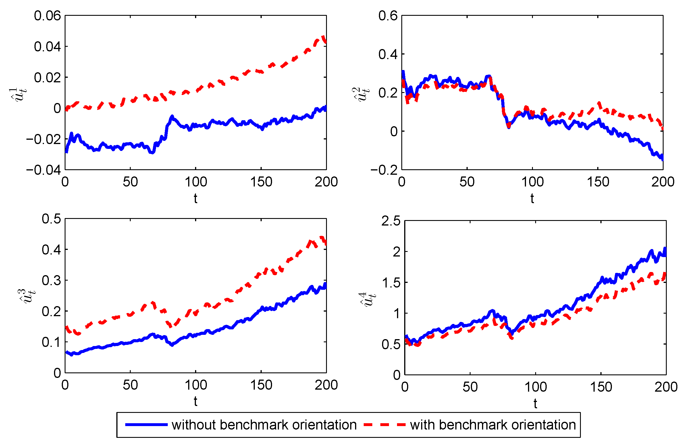
As shown in Figure 3, when the investors have a larger risk aversion coefficient ${\eta }_T=100$, the benchmark process leads to a significant impact on the time-consistent strategy, especially for the investment strategy in the later periods. In this situation, the investors might tend to choose a conservative investment strategy to imitate the return of the benchmark process.

To evaluate whether the time-consistent strategy that considers the benchmark can imitate the return of the benchmark or not, we will give a more intuitive simulation to verify this conclusion. In addition to the condition of Case I, we also suppose that ${\eta }_T=100$, then the return of the portfolio at the different time periods can be derived. As shown in Figure 4, we can find that the return of the benchmark has almost the same trend as that of the proposed portfolio. This results indicate that, when the investors have the larger risk aversion coefficients, the proposed time-consistent strategy can indeed imitate the return of the benchmark.

4.2. The Time-Consistent Strategy with Only Risky Assets

In this section, we will discuss the evolution of the time-consistent strategy with only risky assets. Similar to Section 4.1, we can derive the corresponding path of the time-consistent strategy. The details see Figure 5, Figure 6, Figure 7 and Figure 8.

Suppose that ${\eta }_T=2$ and $q=1.005$. We will compare the time-consistent strategy with and without intertemporal restrictions (i.e., Case I and Case II). As shown in Figure 5, when the intertemporal restrictions are considered in the investment decision, the investors will shrink investment position (i.e., shrinking the short position ${\widehat{u}}_t^1$ and the long position ${\widehat{u}}_t^2$, meanwhile, increasing the long position ${\widehat{u}}_t^3$ and ${\widehat{u}}_t^4$) invested in the risky assets compared to the investment strategy without considering intertemporal restrictions. Unlike the time-consistent strategy with both multiple risky assets and a risk-free asset (e.g., the investors can reduce the portfolio risk by increasing the amount investment in the risk-free asset), when there are only risky assets, the investors can only reduce the investment risk that existed in the earlier periods by adjusting the investment position among the risky assets. Similarly, with the increase in the time period, the position difference of the time-consistent strategies with and without intertemporal restrictions is decreases.

Similar to Figure 2 and Figure 3, we also suppose that ${\eta }_T=2or100$ and $q=1.005$. In the following, we will compare the time-consistent strategies with and without benchmark orientation (i.e., Case I and Case III) to show the impact of the benchmark on the time-consistent strategy. Figure 6 and Figure 7 show that the benchmark will lead to a significant impact on the time-consistent strategy regardless of whether the investors have small risk aversion coefficients or large risk aversion coefficients. Additionally, comparing Figure 2 and Figure 3 and Figure 6 and Figure 7, we can find that, the benchmark has a larger impact on the time-consistent strategy with only risky assets compared to that on the time-consistent strategy with both a risk-free asset and multiple risky assets.

In addition to the condition of Case I, we also suppose that ${\eta }_T=100$. As shown in Figure 8, we can find that the return of the benchmark and the return of the proposed portfolio have almost the same trend, which is consistent with the conclusion shown in Figure 4. This result indicates that, when the investors have the larger risk aversion coefficient, the proposed time-consistent strategy can also imitate the return of the benchmark.

5. Conclusions

In this paper, we investigate a generalized multiperiod mean-variance portfolio optimization with consideration of benchmark orientation and intertemporal restrictions. Since the proposed model is a time-inconsistent problem, we cannot directly solve it by using the traditional dynamic programming approach. Although this problem can be solved indirectly by the embedding scheme, this approach cannot guarantee that the derived strategy (i.e., precommitment strategy) satisfies the time-consistency. Thus, the precommitment strategy has been criticized for lacking rationality by some researchers. In this paper, we adopt a game approach to solve the proposed model, in which the investment decision-making process is deemed to be a noncooperative game. We assume that there exist T players who stand in the different time periods; they all aim to maximize their own generalized mean-variance sub-objectives. Then, the Nash equilibrium solution of this game problem is defined as the time-consistent strategy for the proposed model. In this framework, we derive the time-consistent strategies for the proposed model with and without a risk-free asset by using the backward induction approach. We find that the time-consistent strategy, when there exists a risk-free asset in the capital pool, is feedback one on the benchmark process; when the capital pool with only risky assets, the time-consistent strategy is double feedback one on both benchmark process and wealth process. Finally, we also provide some numerical simulations to show the conclusions derived in this study. These results indicate that, the proposed time-consistent strategy not only can reduce the risk existed in the intermediate process of investment but also can imitate the return of benchmark process.

Apparently, the above game approach can be extended to many time-inconsistent dynamic optimization problems. More importantly, this approach can provide a more suitable strategy for sophisticated decision-makers, since it takes possible future revisions into account. Roughly speaking, the current work can be further extended from the following two aspects. First, this paper assumes that the risk aversion coefficient is independent with current wealth; however, in some cases, the risk aversion coefficient of investors also depends on their level of wealth. Intuitively, the greater the wealth of investors, the less risk averse they are likely to be. Therefore, the case when the risk aversion depends dynamically on current wealth is worth to be investigated in the further work. Second, we can introduce the Markov chain into our proposed model to investigate the time-consistent strategy under the regime switching environment.

References

- Markowitz, H. Portfolio selection. J. Financ. 1952, 7, 77–91. [Google Scholar]
- Li, D.; Ng, W.L. Optimal dynamic portfolio selection: Multiperiod mean-variance formulation. Math. Financ. 2000, 10, 387–406. [Google Scholar] [CrossRef]
- Leippold, M.; Trojani, F.; Vanini, P. A geometric approach to multiperiod mean variance optimization of assets and liabilities. J. Econ. Dyn. Control 2004, 28, 1079–1113. [Google Scholar] [CrossRef] [Green Version]
- Wei, S.-Z.; Ye, Z.-X. Multi-period optimization portfolio with bankruptcy control in stochastic market. Appl. Math. Comput. 2007, 186, 414–425. [Google Scholar] [CrossRef]
- Yao, H.; Zeng, Y.; Chen, S. Multi-period mean–variance asset–liability management with uncontrolled cash flow and uncertain time-horizon. Econ. Model. 2013, 30, 492–500. [Google Scholar] [CrossRef]
- Chen, Z.; Li, G.; Zhao, Y. Time-consistent investment policies inmarkovian markets: A case of mean–variance analysis. J. Econ. Dyn. Control 2014, 40, 293–316. [Google Scholar] [CrossRef]
- Cui, X.; Li, D.; Li, X. Mean-variance policy for discrete-time cone-constrained markets: Time consistency in efficiency and theminimum-variance signed supermartingale measure. Math. Financ. 2017, 27, 471–504. [Google Scholar] [CrossRef]
- Liu, J.; Chen, Z. Time consistent multi-period robust risk measures and portfolio selection models with regime-switching. Eur. J. Opt. Res. 2019, 268, 373–385. [Google Scholar] [CrossRef]
- Zhou, Z.; Zeng, X.; Xiao, H.; Ren, T.; Liu, W. Multiperiod portfolio optimization for asset-liability management with quadratic transaction costs. J. Ind. Manag. Optim. 2019, 15, 1493–1515. [Google Scholar] [CrossRef]
- Roll, R. A mean/variance analysis of tracking error. J. Portf. Manag. 1992, 18, 13–22. [Google Scholar] [CrossRef]
- Zhao, Y. A dynamic model of active portfolio management with benchmark orientation. J. Bank. Financ. 2007, 31, 3336–3356. [Google Scholar] [CrossRef]
- Espinosa, G.E.; Touzi, N. Optimal investment under relative performance concerns. Math. Financ. 2015, 25, 221–257. [Google Scholar] [CrossRef]
- Zhu, S.S.; Li, D.; Wang, S.Y. Risk control over bankruptcy in dynamic portfolio selection: A generalized mean-variance formulation. IEEE Trans. Autom. Control 2004, 49, 447–457. [Google Scholar] [CrossRef]
- Costa, O.; Nabholz, R.d.B. Multiperiod mean-variance optimization with intertemporal restrictions. J. Optim. Theory Appl. 2007, 134, 257. [Google Scholar] [CrossRef]
- Costa, O.L.; Araujo, M.V. A generalized multi-period mean–variance portfolio optimization with Markov switching parameters. Automatica 2008, 44, 2487–2497. [Google Scholar] [CrossRef]
- Costa, O.L.; de Oliveira, A. Optimal mean–variance control for discrete-time linear systems with Markovian jumps and multiplicative noises. Automatica 2012, 48, 304–315. [Google Scholar] [CrossRef]
- Cui, X.; Li, X.; Li, D. Unified framework of mean-field formulations for optimal multi-period mean-variance portfolio selection. IEEE Trans. Autom. Control 2014, 59, 1833–1844. [Google Scholar] [CrossRef]
- Zhou, Z.; Xiao, H.; Yin, J.; Zeng, X.; Lin, L. Pre-commitment vs. time-consistent strategies for the generalized multi-period portfolio optimization with stochastic cash flows. Insur. Math. Econ. 2016, 68, 187–202. [Google Scholar] [CrossRef]
- Celikyurt, U.; Özekici, S. Multiperiod portfolio optimization models in stochastic markets using the mean–variance approach. Eur. J. Oper. Res. 2007, 179, 186–202. [Google Scholar] [CrossRef]
- Yao, H.; Li, Z.; Li, D. Multi-period mean-variance portfolio selection with stochastic interest rate and uncontrollable liability. Eur. J. Oper. Res. 2016, 252, 837–851. [Google Scholar] [CrossRef]
- Björk, T.; Murgoci, A. A General Theory of Markovian Time Inconsistent Stochastic Control Problems. 2010. Available online: http://ssrn.com/abstract=1694759 (accessed on 5 July 2019).[Green Version]
- Basak, S.; Chabakauri, G. Dynamic mean-variance asset allocation. Rev. Financ. Stud. 2010, 23, 2970–3016. [Google Scholar] [CrossRef]
- Wu, H.; Chen, H. Nash equilibrium strategy for a multi-period mean–variance portfolio selection problem with regime switching. Econ. Model. 2015, 46, 79–90. [Google Scholar] [CrossRef]
- Cui, X.; Li, D.; Shi, Y. Self-coordination in time inconsistent stochastic decision problems: A planner–doer game framework. J. Econ. Dyn. Control 2017, 75, 91–113. [Google Scholar] [CrossRef]
- Bensoussan, A.; Wong, K.; Yam, S.C.P.; Yung, S.P. Time-consistent portfolio selection under short-selling prohibition: From discrete to continuous setting. SIAM J. Financ. Math. 2014, 5, 153–190. [Google Scholar] [CrossRef]
- Björk, T.; Murgoci, A. A theory of Markovian time-inconsistent stochastic control in discrete time. Financ. Stoch. 2014, 18, 545–592. [Google Scholar] [CrossRef]
- Zhou, Z.; Liu, X.; Xiao, H.; Ren, T.; Liu, W. Time-consistent strategies for multi-period portfolio optimization with/without the risk-free asset. Math. Probl. Eng. 2018, 2018, 1–20. [Google Scholar] [CrossRef]
- Wang, L.; Chen, Z. Stochastic game theoretic formulation for a multi-period DC pension plan with state-dependent risk aversion. Mathematics 2019, 7, 108. [Google Scholar] [CrossRef]
Figure 1.
The time-consistent strategies with and without intertemporal restrictions.
Figure 2.
The time-consistent strategies with and without benchmark orientation.
Figure 3.
Figure 4.
Figure 5.
Figure 6.
Figure 7.
Figure 8.
© 2019 by the authors. Licensee MDPI, Basel, Switzerland. This article is an open access article distributed under the terms and conditions of the Creative Commons Attribution (CC BY) license (http://creativecommons.org/licenses/by/4.0/).
Share and Cite
MDPI and ACS Style
Xiao, H.; Ren, T.; Zhou, Z. Time-Consistent Strategies for the Generalized Multiperiod Mean-Variance Portfolio Optimization Considering Benchmark Orientation. Mathematics 2019, 7, 723. https://0-doi-org.brum.beds.ac.uk/10.3390/math7080723
AMA Style
Xiao H, Ren T, Zhou Z. Time-Consistent Strategies for the Generalized Multiperiod Mean-Variance Portfolio Optimization Considering Benchmark Orientation. Mathematics. 2019; 7(8):723. https://0-doi-org.brum.beds.ac.uk/10.3390/math7080723
Chicago/Turabian StyleXiao, Helu, Tiantian Ren, and Zhongbao Zhou. 2019. "Time-Consistent Strategies for the Generalized Multiperiod Mean-Variance Portfolio Optimization Considering Benchmark Orientation" Mathematics 7, no. 8: 723. https://0-doi-org.brum.beds.ac.uk/10.3390/math7080723
Note that from the first issue of 2016, this journal uses article numbers instead of page numbers. See further details here.