Analyzing the Causality and Dependence between Gold Shocks and Asian Emerging Stock Markets: A Smooth Transition Copula Approach

Abstract

This study aims to investigate the causality and dependence structure of gold shocks and Asian emerging stock markets. The positive and negative shocks of gold prices are quantified, and Granger causality-based Vector autoregressive and Copula approaches are employed to measure the causality and contagion effect, respectively, between the positive and negative gold shocks and Asian emerging stock markets’ volatilities. In addition, the nonlinear link between gold and stock markets is of concern and this motivates us to propose a Smooth Transition Dynamic Copula that allows for the structural change in time-varying dependence between gold shocks and Asian stock markets’ volatilities. Several Copula families are also considered, and the best-fit Copula model is used to explain the correlation or contagion effects. The findings of the study show that there is some significant causality between gold shocks and Asian stock markets’ volatilities in some parts of the sample period. We also observe a stronger correlation during the global financial crisis when compared to the pre- and post-crisis periods. In addition, the tail dependence is found between Indian stock and negative gold shock and between Korean stock and negative gold shock, which indicated the existence of the risk contagion effects between gold and these two stock markets.

1. Introduction

The Asian emerging stock markets have become increasingly integrated with the global economy in recent years, particularly after the launch of the Emerging Markets Asia Index. The size of these Asian economies covers 20% of the world economy. It is well known that the stock market is important in the development of the Asian emerging economies, as the businesses could issue their shares to mobilize capital from the public investors. Thus, the Asian stock market indices are considered to be a leading indicator of the health of the Asian emerging economies. Nowadays, many investors have considered these emerging markets as the alternative markets for investment, which can provide an excellent opportunity for gaining a higher profit. Although these markets can offer higher gains to investors due to rapid economic growth, they also provide a higher investment risk due to commodity price volatility, economic and financial uncertainty, and an ongoing slowdown in the world economy [1]. This indicates that the Asian emerging stock markets may expose the investors to various risks.

Nguyen et al. [2] and Pastpipatkul, Yamaka, and Sriboonchitta [3] suggested investing in the gold market since gold is generally perceived as a reliable asset and a safe haven commodity hardly hit by the macroeconomic storms to handle and mitigate the risk in the stock market, especially during the extreme market downturn. However, as a commodity, gold’s price depends on the industrial supply and demand, which are unpredictable, as evident from the previous gold shocks with impacts on the stock markets. Therefore, investigating the interconnection between gold shocks and the stock markets is crucial, because this relationship is relevant as a reference source for portfolio management and hedging strategies. Recently, the relationship between the gold and stock returns has received significant attention from many scholars in both literature and empirical fields. However, many studies provide unclear and inconclusive results.

Only a few dealt with the interaction between gold shock and stock market volatility, even though many empirical studies have been conducted to investigate the relationship between gold and stock markets, such as Do, McAleer, and Sriboonchitta [4]; Chen and Wang [5]; Liao, Qian, and Xu [6]; and, Wen and Cheng [1]. It is relevant to distinguish between positive and negative gold shocks, as this permits measuring whether the stock market volatility reacts in different ways to the gold price increases or decreases. Our initial hypothesis is that the gold shock and the stock volatility have a negative relationship when gold acts as a hedging asset, and a positive one when gold cannot act as a hedging asset. It is possible for gold to offer positive returns when equities are at an extreme loss. This way, investors who hold gold in their portfolios will shield themselves from extreme losses in the falling stock market. Therefore, we identify gold shocks by decomposing the gold volatility into positive and negative shocks in this study. Furthermore, we also examine the hedging effects of gold shocks on the Asian emerging stock markets.

Methodologically, we will examine the causality and risk contagion effect between Asian emerging stock markets’ volatility and the gold price shocks while using Granger causality test-based vector autoregression (VAR) model and Copula approach, respectively. In the field of finance, the terms contagion and causality are commonly used interchangeably. The definitions of these two words and their difference are explained in Gulzar at al. [7] and Xu and Gao [8].

Our empirical results show there was volatility causality running from most of the Asian emerging stock markets to the gold market in some periods. We also find that the correlation of some pairs is relatively stronger during the financial crisis compared to the normal periods. Our results also show that gold can be used as an investment hedge in the Saudi Arabian and Qatari stock markets, as a positive gold shock is negatively related to these two stock markets’ volatilities. Therefore, investors can prepare themselves to avoid investment risk in advance, with their understanding of such characteristics of causal effect and dependence.

We organize the rest of the study, as follows: Section 2 provides a review of related studies, Section 3 describes our data and methodology, Section 4 presents empirical results and discussion, and Section 5 concludes the study.

2. Literature Review

In recent years, the emerging stock markets have shown growth in value and volume, providing greater investment chances and drawing substantial capital inflows [9]. However, they are subject to considerable global risks and uncertainty of extreme events. They can offer a new and higher-return investment opportunity from their economic boom when compared to the advanced stock market, but with lower liquidity, thereby implying higher stock volatility. Thus, investors who attempt to long stocks in an illiquid market could be exposed to substantial risks. To prevent this risk, gold can be viewed as one of the hedging or safe haven assets for stock markets under the uncertainty of an occurring event, like the financial crises [10].

The modern portfolio theory of Markowitz can explain the linkage between gold and stock [11] for the construction of an optimal portfolio by maximizing the expected return for a given level of risk. The basic idea behind this concept is to combine risky assets (e.g., stock) with less risky or risk-free assets (e.g., gold or bond) in the portfolio. This framework can also be used to determine the attractiveness of stock relative to gold. Besides, according to Markowitz [11], the riskiness of individual assets, as well as the effects of economic factors, can explain the portfolio diversification. Therefore, the dynamics in various assets and their classes may reflect different responses to the on-going economic fundamentals. For example, the stock market during the financial crisis was expected to pose a higher risk of loss to investors and thereby causing the movement of funds from the stock market to the safe haven market, like gold. Thus, the gold price will further increase due to the higher demand for gold during the financial crisis [12].

Many studies have analyzed the Granger causality between these two markets. Mishra, Das, and Mishra [13] attempted to investigate the causality and causal effect between gold price and stock market returns in India. They revealed that there exists the bidirectional causality relationship between these two variables along the 1991–2009 sample period. Similarly, the work of Bhunia and Das [14] provided evidence supporting the bidirectional causality between the gold price and Indian stock market return during and after the financial crisis in 2007–2008. However, Hussin et al. [15] studied the relationship between the gold price and the Malaysian stock market return and found that gold price is not an appropriate predictor of Malaysian stock price movement. Choudhry, Hassan, and Shabi [16] investigated co-movements between gold returns and volatilities of the UK, US, and Japan stock markets during the global financial crisis. They revealed that there is the bidirectional interdependence between gold returns and the three stock markets’ volatilities, which indicates that gold might not act as the hedging asset for the UK, US, and Japan stock markets during the financial crisis period. However, they mentioned that gold could be used as a hedge against stock markets during the normal economic condition. Additionally, Mensi et al. [17] studied the correlations and volatility spillovers between the S&P 500 and commodity price indices for energy, food, and gold. They found a significant transmission between the S&P 500 and commodity markets, and found that the S&P 500-gold index pair exhibits a high conditional correlation along the sample period. Hood and Malik [18] studied the role of gold in handling volatility as a hedge and safe haven from November 1995 to November 2010 and found that gold represents a weak safe haven for the US stock market.

As for the measurement of the contagion effect, the most classical method is based on Pearson’s [19] correlation coefficient, which only describes a static linear correlation between the variables. Thus, Engle [20] introduced the Dynamic Conditional Correlation GARCH model to measure the time-varying correlation between the variables. Later, this model has gained increasing interest from researchers and practitioners. Chen and Wang [5] used DCC-GARCH to examine the dynamic relationships between gold and stock markets in China. They found that gold acts as a safe haven for only the market downturns analyzed, while gold does not offer good risk hedging in the market upturns. Basher and Sadorsky [21] considered various DCC-GARCH-type models, namely DCC-GARCH, GO-GARCH, and ADCC-GARCH, to investigate the dynamic correlation. In general, they revealed that gold has a positive correlation with emerging stock market growth. Thus, gold might not be good hedging for emerging stock markets.

Recently, many researchers have questioned the DCC-GARCH performance, as there is evidence that the dependencies between financial variables are non-linear and asymmetric. Therefore, the Copula method has been introduced to measure the contagion or co-movement between two or more variables. Copula was firstly introduced by Sklar [22] and further developed and described by Jo [23] and Nelson [24]. This model has been widely used to examine the contagion between gold and stock markets. Do, McAleer, and Sriboonchitta [4] studied the impact of gold on the volatility of the ASEAN emerging stock market. They employed a GARCH to model the stock volatility and showed that gold should be a substitute commodity for Indonesian and Philippine stock markets, while in Indonesia, Thailand, and Malaysia, it can be a complementary commodity for stocks. Recently, the Copula-based GARCH method has been of great interest to researchers. It is widely used to measure the contagion effects between stock markets and gold markets. Among others, Nguyen et al. [2], Pastpipatkul, Yamaka, and Sriboonchitta [25,26], and Beckmann, Berger, and Czudaj [27] used different Copula functions to test the correlation between gold and stock.

With the improvement of research methodology, many studies have found that the dependencies between financial variables are no--linear and asymmetric. Patton [28] proposed the Dynamic Copulas for capturing the time-varying dependence structures, which represent an essential improvement when compared to the static Copula. The Dynamic Copula framework is extended by Silva Filho, Ziegelmann, and Dueker [29] and Fei, Fuertes, and Kalotychou [30] to accommodate time-varying dependence and non-linearity. They constructed the Markov Switching Dynamic Copula (MSDC) model to measure the dependence structure of the financial contagion. There are several advantages in adopting this approach. First, the crisis and non-crisis periods can be detected by the Hidden Markov process of Hamilton’s filter [31]. Second, it is more efficient in capturing the structural change of the dynamic dependency structures among different markets. However, the existing MSDC Copula model is likely to have two marked limitations. First, the MSDC model assumes the first-order Markov chain, i.e., the current state variable depends on its immediate past value. Nevertheless, this assumption is not likely to hold as the long memory of the regime change might exist. Additionally, the model incorporates less prior information regarding the switching process. The switching process then might not reflect the real non-linear structure of dependence between financial variables. Second, the transition function of the MSDC relies on a filtered probability and it does not incorporate the threshold variable. Thus, the information about the threshold point or breakpoint in the MSDC is unavailable [32].

This study introduces both methodological and empirical contributions to the literature to deal with the limitation of the MSDC. In the former, we apply the logistic transition function of Silvennoinen and Teräsvirta [33] to the dynamic copula model and propose a smooth logistic transition copula. The appealing feature of this model is its ability to capture the gradual changes and the sudden transition of the dependence patterns. This method will allow for the dependence structure between random variables to vary across different regimes. This dependence measure resembles the threshold (or change point) and smooth parameter. To this end, the Smooth Transition Dynamic Copula model is proposed in this study.

Through summarizing the previous literature, there are various methods that are used for testing causality, and investigating the contagion effect, and each method has its advantages and disadvantages. Methodologically, the present study investigates the causality using the Granger causality test based on the VAR model, and proposes using the Smooth Transition Dynamic Copula model to explore the contagion effect. Furthermore, all of the studies reviewed above concerning the impact of gold on the stock market use gold price, gold return, or gold volatility as a proxy, which might not yield the accurate results. If the tail dependence between gold and stock exists, these proxies will not be able to explain extreme market events properly. Hence, it is of interest to address the positive and negative gold price shocks to find out whether they have different or asymmetric impacts on stock volatility in the stock markets.

The following three aspects mainly reflect the overall contribution of this paper. First, we consider the Granger causality test to examine the causality of risk spillover effect between gold shocks and the Asian emerging stock markets’ volatilities. It is not clear whether the Asian emerging stock market volatility is being anticipated by gold price shocks or the gold price shocks are just a consequence of the Asian emerging stock markets’ volatility. To disentangle these effects, a Granger causality analysis of the stock volatility and different lags and leads to gold price shocks would be very informative. Second, we propose a Smooth Dynamic Copula model to describe the nonlinear and asymmetric dependency structure, as well as to obtain the lower tail coefficients, which can adequately depict the risk of the contagion effect. Using the tail coefficients to measure the risk contagion from gold shocks to different Asian emerging stock markets is also an innovative approach of this study when compared with previous studies. Additionally, by investigating the variables’ tail dependence, we can gain more information to assist governments to make an appropriate economic policy and help investors to get better risk-return combinations in their portfolio diversification. Thirdly, many scholars, often focusing on the advanced stock markets, have already explored the relationship between the volatilities of gold and stock returns. However, in this study, we attempt to explore whether or not the gold shocks (positive and negative) will give out any contagion effect on the Asian emerging stock markets.

3. Data and Methodology

3.1. Data

In this study, we consider ten emerging stock markets that are ranked the highest on the basis of their market values. We use weekly time series of gold price and 10 Asian emerging stock indexes of Korea (Korea Composite Stock Price Index; KOSPI), Thailand (Stock Exchange of Thailand Index; SET), China (Shanghai Composite Index; SSEC), Indonesia (Jakarta Stock Exchange Composite; JKSE), India (S&P BSE SENSEX; BSESN), Vietnam (Vietnam Ho Chi Minh Stock Index; VNI), Philippines (Philippine Stock Exchange; PSE), Saudi Arabia (Tadawul All Share Index; TASI), Qatar (Qatar Exchange Index; QE), and Hong Kong ( Hang Seng Index: HSI) throughout 1 January 2001 to 31 December 2018. We took all of the information from every Friday of the week. For weeks that the stock market was closed on Friday, we use the information on Thursday. All of the stock indexes and gold prices are collected from www.investing.com. Returns of gold and stocks are calculated by taking the first difference of the natural logarithm of price and index.

Table 1. Descriptive statistics of the weekly return of the stock market and gold.

SERIES	MEAN	STD	SKEWNESS	KURTOSIS	ADF
GOLD	0.0033	0.2470	−0.1998	4.5683	−31.1167 ***
SSEC	0.0008	0.0335	−0.0423	5.6511	−27.9771 ***
BSESN	0.0028	0.0298	−0.2767	6.0163	−18.6378 ***
JKSE	0.0033	0.0296	−0.6408	7.6383	−31.6757 ***
KOSPI	0.0019	0.0301	−0.3639	8.2530	−32.9096 ***
HIS	0.0010	0.0294	−0.0679	5.5274	−30.4016 ***
PSE	0.0022	0.0278	−0.1281	7.7969	−31.8466 ***
TASI	0.0019	0.0339	−0.9987	9.1291	−28.9613 ***
QE	0.0028	0.0333	−0.1224	8.3156	−28.4976 ***
SET	0.0023	0.0273	−0.9961	10.6266	−12.6105 ***
VNI	0.0023	0.0398	−0.0702	6.8271	−17.4981 ***

Note: ADF is the Augmented Dickey–Fuller unit root test. The null hypothesis is that the variable includes a unit root, and the alternative is that the variable does not include a unit root, which means the variable is stationary. (***) indicates significance at the 1% level.

presents the descriptive statistics of the weekly gold price and the 10 stock market returns. It can be seen that the gold price and Indonesia’s stock return show the highest average return (0.0033), followed by India’s stock return and Qatar’s stock return, respectively. The gold price has the highest standard derivation (0.2470), followed by the stock returns of Vietnam and Saudi Arabia. This finding suggests that gold price has the largest fluctuation and gold is riskier than the Asian emerging stocks. Negative skewness and high kurtosis values are observed in all market and gold returns, which indicated the fat tails in the return distributions and the non-normality of the data series. The Augmented Dickey–Fuller (ADF) test is employed to examine the stationarity of the data series, and the result indicates that all stock and gold returns are stationary.

3.2. Methodology

In this study, we defined the contagion effect as the co-movement of shocks and volatilities [34]. Therefore, we can establish the causality and dependence between the Asian emerging stock markets’ volatilities and positive and negative gold shocks by employing a rich set of quantitative techniques, such as Granger causality and various Copula functions. We first employ the GARCH(1,1) with the skew-t model to quantify the conditional variance or volatility of the stock indices and gold price. Subsequently, we use the Granger causality test to examine the lead-lag relationship between stock market volatilities and gold shocks. Finally, single-regime Copulas and two-regime Copulas are both used to investigate the dependence structure.

3.2.1. Generalized Autoregressive Conditional Heteroscedasticity (GARCH) Model

In this study, GARCH (1,1) with the skew-t specification is used to estimate the volatility of 10 Asian emerging stock markets’ returns and gold return. Let $R_{i,t}$ and ${\sigma }_{i,t}$ be the return and conditional volatility of return i at time t, respectively. We can write the GARCH (1,1) for return i, as

$$R_{i,t}={\mu }_i+{\epsilon }_{i,t},$$

(1)

where ${\mu }_i$ is the constant parameter of the mean equation for return i. ${\epsilon }_{i,t}$ is the error term that can be decomposed, as follows:

$${\epsilon }_{i,t}=\sqrt{{\sigma }_{i,t}}{z}_{i,t},$$

(2)

where ${\sigma }_{i,t}=E\left({\epsilon }_{i,t}^2|{\psi }_{i,t-1}\right)$ is the conditional variance of the error and $z_t={\epsilon }_{i,t}/\sqrt{{\sigma }_{i,t}}$ is the standardized residual following the skew-t distribution $\left(z_t\sim skewed-t(0,1,df,\phi )\right)$. The parameters $df$ and $\phi$ are the degree of freedom and skewness parameters, respectively. ${\psi }_{t-1}$ is the information set that is available at time $t-1$. According to Bollerslev [35], the conditional variance can be predicted by the lagged conditional variance and the square of the error term in the mean equation. In this study, we consider the GARCH (1,1) model to model the volatility, as one lag order can sufficiently capture the volatility clustering of the stock returns [36]. Thus, the conditional variance equation can be written as

$${\sigma }_{i,t}={\alpha }_{i,0}+{\alpha }_{i,1}{\epsilon }_{i,t-1}^2+{\beta }_i{\sigma }_{i,t-1},$$

(3)

where ${\alpha }_{i,0}>0,{\alpha }_{i,1}>0,{\beta }_i>0$ and ${\alpha }_i+{\beta }_i\le 1$. To quantify the shock of gold return, we follow the suggestion of Lee et al. [37] and compute the positive and negative gold shocks as in the followings

$$PG{S}_t=\max [0,{\epsilon }_{Gold,t}/{\sigma }_{Gold,t}],$$

(4)

$$NG{S}_t=\min [0,{\epsilon }_{Gold,t}/{\sigma }_{Gold,t}],$$

(5)

where $PG{S}_t$ and $NG{S}_t$ are the positive and negative gold shocks, respectively.

3.2.2. Granger Causality Test Method

Following the rapid financialization of commodities, Granger causality and contagion effect between gold and stock markets have been empirically tested. As for causality, the most famous method used to examine the causality between two variables is the Granger causality test [38] that is based Vector Autoregressive (VAR) model. This model has the ability to investigate the linear causality and causal effect between variables. Granger causality is a statistical hypothesis test for testing whether a one-time series is useful in forecasting another, according to Granger [38]. Note that the causality between positive and negative gold price shocks; and, Asian emerging stock volatilities are examined, thus the specific testing equations for our study can be presented, as follows:

$$z_{i,t}^{stock}={\displaystyle \sum _{p=1}^P{\varphi }_p^1{z}_{i,t-p}^{stock}+{\displaystyle \sum _{p=1}^P{\delta }_p^{1}PG{S}_{t-p}+u_{i,t}^1},}$$

(6)

$$z_{i,t}^{stock}={\displaystyle \sum _{p=1}^P{\varphi }_p^2{z}_{i,t-p}^{stock}+{\displaystyle \sum _{p=1}^P{\delta }_p^{2}NG{S}_{t-p}+u_{i,t}^2},}$$

(7)

This method is to separate positive and negative price shocks. If the value of the gold price shocks is positive, then we will specify zero in one series and its positive value in the other series. Likewise, we will specify zero in one series and its negative value in the other if the value is negative. To test the causality between two variables in Equations (6) and (7), we can set the null hypothesis $H_0:{\delta }_1={\delta }_2=\dots ={\delta }_p$, while the alternative hypothesis $H_1$: $H_0$ is not valid. To test this hypothesis, the LR-statistic is used. We consider the Akaike information criterion (AIC) to select the optimal lag order of a VAR (p) model in Equations (6) and (7). Subsequently, we choose the best lag while considering the lowest AIC.

3.2.3. Copulas Approaches

The Copula approach measures the correlation between gold price shocks and Asian emerging stock markets’ volatilities. Following Sklar’s theorem [22], two continuous marginals can be joined by the Copula function $C(\cdot )$. Thus, a two-dimensional joint distribution function $H(x,y)$ can be defined, as

$$H(x,y)=C(F_x(x),F_y(y))$$

(8)

where $F_x(x)$ and $F_y(y)$ are the cumulative marginal distribution of random variables $x$ and $y,$ respectively. If $F_x(x)$ and $F_y(y)$ are continuous, the Copula function that is associated with $H(\cdot )$ is unique and might be computed by

$$C(u,v)=H(F_x^{-1}(u),F_y^{-1}(v)),$$

(9)

where $F^{-1}(\cdot )$ is the inverse function. $u$ and $v$ are uniform [0,1] variables, where $u=F_x(x)$ and $v=F_y(y).$ In this study, we aim to find the correlation between gold price shocks and Asian emerging stock volatilities; thus, we can construct the joint distribution of $u_t=F_z(z_{i,t})$ and $v_t^{+}=F_{PGS}(PG{S}_t)$, and the joint distribution of $u_t=F_z(z_{i,t})$ and $v_t^{-}=F_{NGS}(NG{S}_t)$, as in the followings:

$$H(u,v^{+})=H(F_z(z_{i,t}),F_{PGS}(PG{S}_t)),$$

(10)

$$H(u,v^{-})=H(F_z(z_{i,t}),F_{NGS}(NG{S}_t)),$$

(11)

Note that $z_{i,t}$ denotes a standardized residual obtained from the marginal model. There are various Copula functions proposed to join the marginal distributions and the selection of Copula type is essential. In this paper, we use five families of Copulas to consider different patterns of dependence between stock market volatility and the gold shocks. Copula functions commonly used in research are Normal, Student-t, Gumbel, Clayton, and Frank. Additionally, AIC is used as the criterion for selecting the best-fit Copula function.

Table 2. Copula functions.

Copula	Function	Parameter	Kendall’s Tau	Tail Dependence
Normal	$C^G(u,v|\theta )=\Phi \left[{\Phi }^{-1}(u),{\Phi }^{-1}(v)\right].$	$\theta =[-1,1]$	$\frac{2}{\pi }\arcsin (\theta )$	No tail dependence
Student-t	$C^S(u,v|\theta )=T_{\theta }\left[t_{\theta }^{-1}(u),t_{\theta }^{-1}(v)\right].$	$\theta =[-1,1]$	$\frac{2}{\pi }\arcsin (\theta )$	${\lambda }_U={\lambda }_L=2t_{v+1}\left(-\sqrt{v+1}\sqrt{1-\theta /1+\theta }\right)$
Gumbel	$C^{Gu}(u,v|\theta )=\exp (-{({(-\log (u))}^{\theta }+{(-\log (v))}^{\theta })}^{1/\theta }).$	$\theta =[1,\infty ]$	$1-\frac{1}{\theta }$	${\lambda }_L=0$, ${\lambda }_U=2-2^{1/\theta }$
Clayton	$C^{Cl}(u,v|\theta )={(u^{-\theta }+v^{-\theta }-1)}^{-1/\theta }$	$\theta =[0,\infty ]$	$\frac{\theta }{\theta +2}$	${\lambda }_L=2^{-1/\theta }$, ${\lambda }_U=0$
Frank	$C^{Fr}(u,v|\theta )=-\frac{1}{\theta }\log \left[1+\frac{(\exp (-\theta u)-1)(\exp (-\theta v)-1)}{\exp (-\theta )-1}\right]$	$\theta =[-\infty ,\infty ]$	$1-\frac{4}{\theta }+4\frac{D(\theta )}{\theta }$	No tail dependence

Note: $2 < v \le 30$ is the degree of freedom of Student-t Copula. $D$ is the Debye function.

presents the Copula specifications.

3.2.4. Smooth Transition Dynamic Copula Model

We now propose using our Copula model called Smooth Transition Dynamic Copula (STDC) model to capture such nonlinearities in the dependence structure. We extend the single-regime Dynamic Copula of Patton [28] by extending the Smooth Transition model of Silvennoinen and Teräsvirta [33] to the time-varying equation of the Dynamic Copula model. Basically, our model is constructed in a similar way, as introduced in the Markov Switching Dynamic Copula model of Silva Filho, Ziegelmann, and the logistic cumulative distribution function is used to replace the Hamilton’s filtered probability [31]. This function is used as a smooth transition function to allow for the parameters in the time-varying equation to switch across the regimes. Before introducing our model, let us provide a review of the Dynamic Copula model. According to Patton [28], the time-varying equation is constructed from the ARMA (1,m) process

$${\theta }_t=\mathrm{\Lambda }\left({\omega }_0+{\omega }_1{\theta }_{t-1}+{\omega }_2\Gamma \right),$$

(12)

where ${\omega }_0$, ${\omega }_1$, and ${\omega }_2$ are the estimated parameters. $\mathrm{\Lambda }$ is an appropriate transformation function to ensure that the parameter always remains in its interval: $\mathrm{\Lambda }(a)=1-exp(-a){\left(1+exp(-a)\right)}^{-1}$ for Normal and Student-t Copulas, $\mathrm{\Lambda }(a)=exp\left(a\right)$ for Clayton Copula, $\mathrm{\Lambda }(a)=\left(exp\left(a\right)+1\right)$ for Gumbel Copula, and $\mathrm{\Lambda }(a)=a$ for Frank Copula. ${\theta }_t$ is the dependence measure of interest and $\Gamma$ is the forcing variable, which is defined as

$${\Gamma }_t=\left\{\begin{array}{c}\frac{1}{m}{\displaystyle {\sum }_{j=1}^m{F}_1^{-1}(u_{t-j})F_2^{-1}(v_{t-j})\hspace{0.17em}\hspace{0.17em}\hspace{0.17em}\hspace{0.17em}\hspace{0.17em}\hspace{0.17em}\hspace{0.17em}\hspace{0.17em}\hspace{0.17em}\hspace{0.17em}\hspace{0.17em}\hspace{0.17em}\hspace{0.17em}\hspace{0.17em}\hspace{0.17em}\mathrm{Elliptical}}\\ \frac{1}{m}{\displaystyle {\sum }_{j=1}^m\left|u_{t-j}-v_{t-j})\right|\hspace{0.17em}\hspace{0.17em}\hspace{0.17em}\hspace{0.17em}\hspace{0.17em}\hspace{0.17em}\hspace{0.17em}\hspace{0.17em}\hspace{0.17em}\hspace{0.17em}\hspace{0.17em}\hspace{0.17em}\hspace{0.17em}\hspace{0.17em}\hspace{0.17em}\hspace{0.17em}\hspace{0.17em}\hspace{0.17em}\hspace{0.17em}\hspace{0.17em}\mathrm{Archimedean}.}\end{array}\right.$$

(13)

We generalize the single-regime Copula dependence in Equation (12) by introducing the logistic transition function $G\hspace{0.17em}({\theta }_t,\gamma ,\mathsf{\Upsilon })$, which is assumed to be continuously differentiable with respect to the speed of smoothness $(\gamma )$ and threshold $(\mathsf{\Upsilon })$ parameters. Hence, the time-varying equation of STDC can be written as

$${\theta }_t=\mathrm{\Lambda }\left({\omega }_{01}+{\omega }_{02}{\theta }_{t-1}+{\omega }_{03}\Gamma +\left(\left({\omega }_{11}+{\omega }_{12}{\theta }_{t-1}+{\omega }_{13}\Gamma \right)\cdot G\hspace{0.17em}\left({\theta }_{t-1},\gamma ,\mathsf{\Upsilon }\right)\right)\right),$$

(14)

where the logistic transition function is defined as

$$G\hspace{0.17em}{({\theta }_{t-1},\gamma ,\mathsf{\Upsilon })}_t={(1+\exp [-\gamma ({\theta }_{t-1}-\mathsf{\Upsilon })])}^{-1},$$

(15)

where ${\theta }_{t-1}$ is the dependence parameter at time t-1 or the threshold variable. Note that, when $\gamma \to \infty$, our proposed model becomes the sudden-switch Dynamic Threshold Copula. When $\gamma \to 0$, our model becomes the single-regime Dynamic Copula of Patton [28].

We use the Inference function margins (IFM) method to estimate this model. Thus, the estimation of the STDC is conducted in two steps: First, we estimate the marginal parameters that are based on GARCH (1,1) with skew-t. Second, we fix the estimated marginal parameters in the Copula likelihood function and estimate the dynamic Copula parameters. The statistical properties of this estimation procedure can be found in Patton [28].

4. Empirical Results and Discussion

4.1. GARCH-skew-t Model Results

We present the estimates, by the GARCH (1,1) conditional volatility model, of the returns of the 10 Asian emerging stock markets and gold in

Table 3. Estimates by GARCH (1,1)-skew-t model for the returns of ten stocks and gold.

Parameter Estimation	${\mathit{\mu }}_{\mathit{i}}$	${\mathit{\alpha }}_{\mathit{i},0}$	${\mathit{\alpha }}_{\mathit{i},1}$	${\mathit{\beta }}_{\mathit{i}}$	$\mathit{d}\mathit{f}$	$\mathit{\phi }$	Log-likelihood	Q(10)	ARCH(1)-LM
SSEC	0.0003 * (0.0001)	<0.0001 * (<0.0001)	0.1231 * (0.0279)	0.8604 * (0.0284)	5.3588 * (1.3354)	0.9413 * (0.0248)	1903.939	0.2280	0.8993
BSESN	0.0033 * (0.0004)	<0.0001 (<0.0001)	0.0987 * (0.0231)	0.8895 * (0.0262)	13.5783 * (5.058)	0.8665 * (0.0429)	2022.767	0.4269	0.6320
JKSE	0.0034 * (0.0008)	<0.0001 (<0.0001)	0.1243 * (0.0326)	0.8481 * (0.0429)	4.3589 * (0.9547)	0.9322 * (0.0427)	2003.342	0.0792	0.9815
KOSPI	0.0016 * (0.0007)	<0.0001 * (<0.0001)	0.1286 * (0.0295)	0.8567 * (0.0344)	7.8885 * (2.0185)	0.7866 * (0.0368)	2044.873	0.5249	0.6271
HIS	0.0019 * (0.0008)	<0.0001 * (<0.0001)	0.0855 * (0.0205)	0.8927 * (0.0248)	12.8507 * (4.3224)	0.9041 * (0.0469)	2013.785	0.7588	0.8403
PSE	0.0028 * (0.0008)	<0.0001 (<0.0001)	0.1081 * (0.0344)	0.8568 * (0.0488)	6.7247 * (1.2758)	0.9536 * (0.047)	2033.291	0.4216	0.6623
TASI	0.0029 * (0.0007)	<0.0001 * (<0.0001)	0.3271 * (0.0490)	0.6348 * (0.0409)	4.5519 * (0.6832)	0.8688 * (0.0433)	1972.510	0.0060	0.9464
QE	0.0024 * (0.0008)	<0.0001 * (<0.0001)	0.2589 * (0.0578)	0.6832 * (0.0670)	3.9941 * (0.6088)	1.0567 * (0.0461)	1960.371	0.1001	0.2883
SET	0.0019 * (0.0007)	<0.0001 (<0.0001)	0.0803 * (0.0192)	0.9145 * (0.0199)	6.3371 * (1.2102)	0.8455 * (0.0401)	2070.848	0.5220	0.3001
VNI	0.0002 * (0.0001)	<0.0001 * (<0.0001)	0.3461 * (0.0634)	0.6741 * (0.0517)	5.6696 * (0.9806)	0.9692 * 0.0486)	1861.425	0.4001	0.4539
GOLD	0.0025 * (0.0001)	<0.0001 * (<0.0001)	0.0487 * (0.0300)	0.9110 * (0.0749)	11.9145 * (4.3710)	0.8505 * (0.0412)	1598.22	0.2368	0.5981

Note: (*) stands for statistical significance at the 5% level. Q(10) is the Ljung–Box Q statistic for the null hypothesis that there is no autocorrelation up to order 10 for the standardized residuals.

. All of the estimates of the parameters are obtained while using MLE. All of the coefficients in the variance equations i.e., the intercept (${\alpha }_{0,i}$), the ARCH effects $({\alpha }_{1,i})$, and the GARCH effects $({\beta }_i)$ are positive and highly significant, which indicates that all stock indices and gold price exhibit high volatility persistence. Note that the ARCH effects and GARCH effects represent the effects of the past error term and its past volatility on current volatility, respectively. Afterwards, the goodness-of-fit is conducted to test whether the obtained standardized residuals have no autocorrelation and heteroscedasticity. The Ljung–Box Q statistic at lag 10 (Q10) and ARCH-LM at lag 1 (ARCH(1)-LM) are respectively used for those purposes. As shown in columns 9 and 10 in Table 3, the p-values for Q(10) of autocorrelation test and ARCH(1)-LM test of heteroscedasticity are greater than 0.05, which indicate that there are no autocorrelation and heteroscedasticity of the standardized residuals.

4.2. Estimates of Causality Using Granger Causality Test

Table 4. Granger causality test for the relationship between gold price shocks and stock returns.

	Stock→PGS		PGS→Stock		Stock→NGS		NGS→Stock
	p-Value	Causality	p-Value	Causality	p-Value	Causality	p-Value	Causality
SSEC	0.2894	No	0.4818	No	0.1989	No	0.1282	No
BSESN	0.6213	No	0.3218	No	0.0197	Yes	0.6562	No
JKSE	0.7206	No	0.1132	No	0.028	Yes	0.1158	No
KOSPI	0.8298	No	0.4675	No	0.0212	Yes	0.9489	No
HIS	0.2820	No	0.4307	No	0.0297	Yes	0.2071	No
PSE	0.6704	No	0.2625	No	0.4443	No	0.3753	No
TASI	0.4239	No	0.6444	No	0.2021	No	0.6505	No
QE	0.8411	No	0.3134	No	0.3490	No	0.4286	No
SET	0.9868	No	0.6758	No	0.0485	Yes	0.0275	Yes
VNI	0.3177	No	0.6069	No	0.0973	Yes	0.4132	No

Note: (1) represents lag 1. The lag for the VAR model is selected by the Akaike information criterion (AIC).

presents the results of the Granger causality tests. We reject the null hypothesis when the p-value falls below 0.10. Stock→PGS indicates the null hypothesis that stock volatility does not Granger-cause positive gold price shock, whereas PGS→Stock indicates that the null hypothesis of that positive gold price shock does not cause stock volatility. Likewise, Stock→NGS and NGS→Stock point out the Granger causality between negative gold price shock and stock volatility. The results of causal relationships between the gold price shocks and the Asian emerging stock markets’ volatilities can be summarized in three parts. (1) There is no Granger causality between the positive gold shock and the Asian emerging stock markets’ volatilities. (2) A unilateral Granger causality is found from stock market volatility to negative gold shock for the cases of Indonesia, India, Korea, Hong Kong, and Vietnam. (3) The bidirectional causality between the stock market volatility and negative gold shock is found in the case of Thailand (SET). Therefore, we can conclude that there is no causality between the Asian emerging stock markets’ volatility and positive gold shock. However, there is weak evidence of the causal relationship between Asian emerging stock markets’ volatilities and negative gold shock.

4.3. Estimates of Causality Using the Rolling Window Granger Causality Test

The sample period of almost two decades in this study naturally leads us to think that there might exist a structural change in the causal relationship between the Asian emerging stock markets’ volatilities and gold shocks. In other words, the causal relationships between the two considered variables may change over time and the structural change might affect temporal Granger causality effects that can be sensitive to the sample period adopted [39]. Thus, in this section, the rolling window Granger causality test is considered to investigate the time-varying Granger causality. The temporal stability of the parameters in the Granger causality-based VAR model is examined to confirm the structural change effect in Granger causality. We conduct the Sup-F test that was introduced by Andrews and Ploberger [40] to examine the stability of the parameters. The null hypothesis is that the parameter is constant, while the alternative hypothesis is that there is regime-switching of parameters. Thus, if the parameters are found to be unstable, then they may cause the pattern of causality to change over time.

Table 5. Parameter stability tests.

	Stock→PGS Eq.		Stock→PGS Eq.		Stock→NGS Eq.		NGS→Stock Eq.
	Sup-F	p-Value	Sup-F	p-Value	Sup-F	p-Value	Sup-F	p-Value
SSEC	18.994	0.000	20.378	0.000	23.661	0.000	24.643	0.000
BSESN	34.778	0.000	36.311	0.000	36.325	0.000	38.197	0.000
JKSE	45.109	0.000	43.318	0.000	47.315	0.000	45.987	0.000
KOSPI	13.125	0.000	12.998	0.000	13.987	0.000	13.547	0.000
HIS	34.477	0.000	32.364	0.000	36.897	0.000	34.211	0.000
PSE	13.288	0.000	11.559	0.000	15.368	0.000	12.331	0.000
TASI	10.548	0.000	9.374	0.000	10.314	0.000	12.887	0.000
QE	8.677	0.000	9.665	0.000	11.556	0.000	13.984	0.000
SET	20.668	0.000	22.365	0.000	24.357	0.000	26.779	0.000
VNI	31.156	0.000	35.664	0.000	33.971	0.000	36.341	0.000

Note: The p- values for all the stability tests computed from parametric bootstrapping.

provides the results of the stability test.

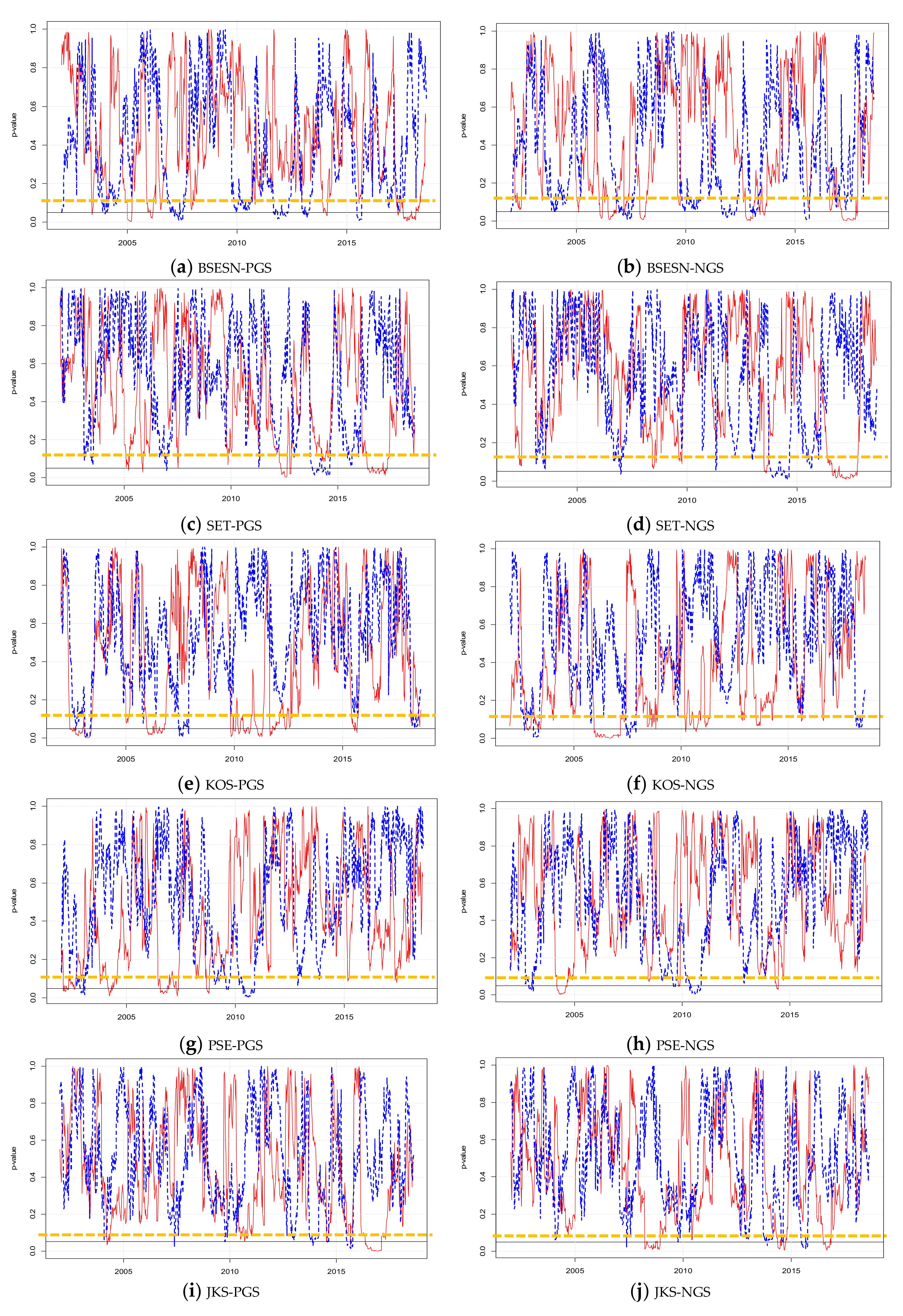
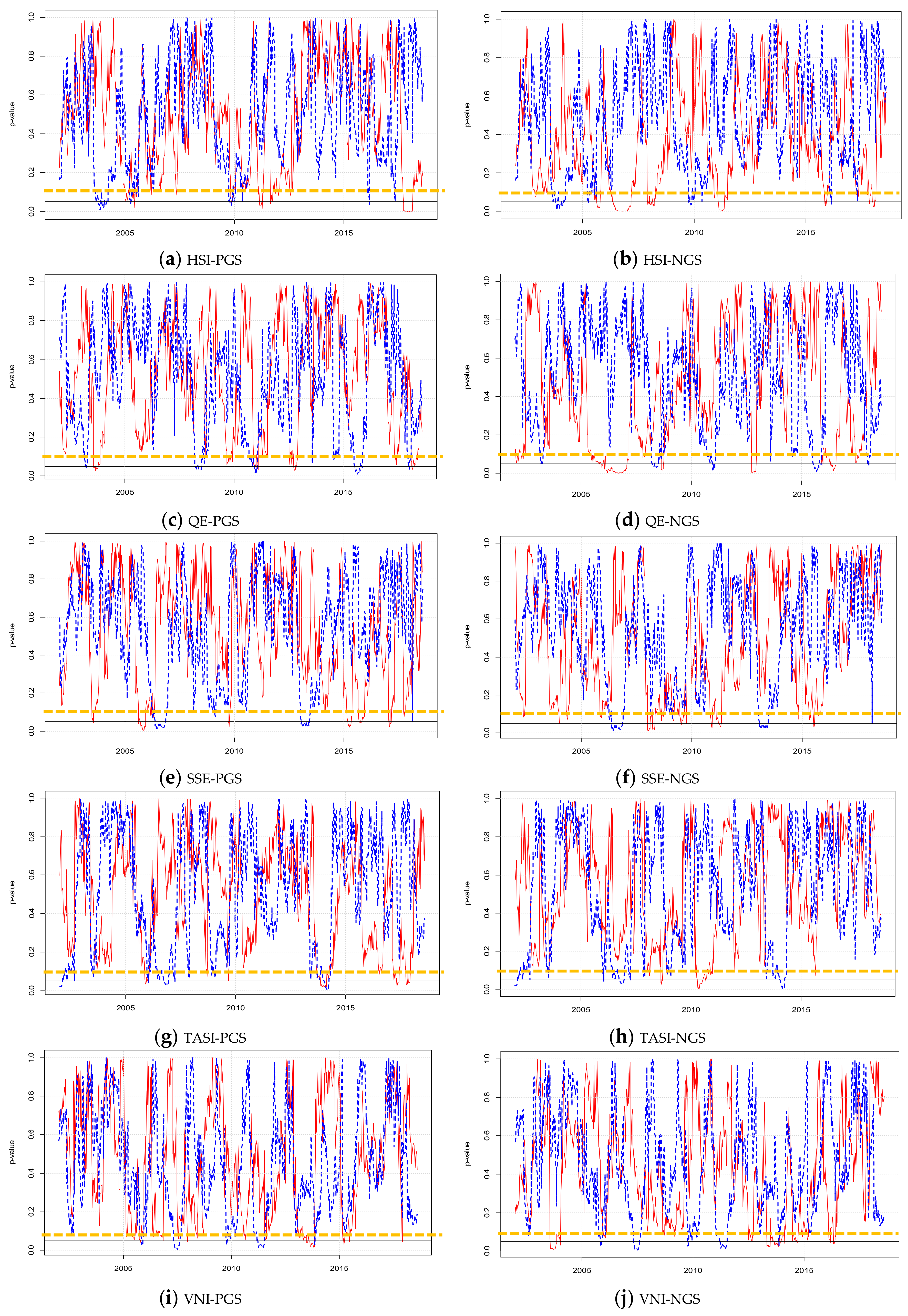
According to Table 5, we can observe that the estimated VAR models for all pairs provide unstable parameters, as the null hypothesis of the Sup-F tests is rejected. This indicates the existence of structural change in the Granger causality-based VAR model, which implies that the results of the full-sample Granger causality reported in Table 4 may not be reliable. Therefore, the additional examination by time-varying Granger causality tests during the sample period is conducive to revealing the time-varying nature of the causality between the Asian emerging stock markets’ volatilities and gold shocks in more detail. We adopt the method that was proposed by Nyakabawo et al. [41] to proceed with the rolling-window Granger causality tests we apply the above testing procedure to rolling subsamples of 52 weeks, approximately one trading year. We test for the presence of Granger causality in the Asian emerging stock markets’ volatilities and gold shocks for all pairs within our sample, and Figure 1 and Figure 2 illustrate the bootstrapped p-values of the rolling test statistics.

Figure 1 and Figure 2 demonstrate the p-values of LR. Note that positive and negative gold shocks are both examined in this section. The left panel of Figure 1 and Figure 2 illustrates the Granger causality stock volatility and positive gold shock, while the right panel of these two figures illustrates the Granger causality stock volatility and negative gold shock. Note that the red line presents the null hypothesis that the stock volatility does not Granger-cause gold shock, while the blue dashed line presents the null hypothesis that the gold shock does not Granger-cause the stock volatility. The solid black line and orange dashed line corresponds to the 5% and 10% significant levels, respectively. We divide our analysis period into three sub-periods, namely pre-crisis (before 1 August 2007), global financial crisis (1 August 2007–31 December 2012), and post-crisis (after 4 January 2013), to gain more interesting Granger causality results [42,43]. According to the results, the Granger causality between positive gold shock and the Asian emerging stock markets’ volatilities can be summarized, as in the following presentation. (1) The estimated p-values substantially change over the sample period for all cases with time-varying values between 0.000 and 1.000. (2) The alternative hypothesis that there is Granger causality effect of each series on the other is accepted during some periods of the sample by using the 10% significant level as the critical level. (3) The null hypothesis that the Asian emerging stock markets’ volatility does not Granger-cause gold shocks (red line) is rejected in some years during the pre-crisis period for BSESN-PGS, PSE-PGS, PSE-NGS, JKS-PGS, HSI-PGS, SSE-PGS, SSE-NGS, TAD-PGS, VNI-PGS, and VNI-NGS pairs. This indicates that seven out of the 10 Asian emerging stock markets’ volatilities had the contagion effect on the gold market before the global financial crisis. Additionally, we can reject the null hypothesis that gold shock does not Granger-cause Asian emerging stock markets’ volatility in some years during 2004–2006 (blue dashed line) for BSESN-PGS, BSESN-NGS, JKS-PGS, JKS-NGS, HSI-PGS, HSI-NGS, and SSE-PGS. (4) During the global financial crisis, the BSESN-NGS, KOS-NGS, JKS-NGS, HSI-NGS, QE-NGS, SSE-NGS, and VNI-NGS pairs are found to have a significant Granger causality effect of stock volatility on negative gold shock. In other words, the stock markets of India, Korea, Indonesia, Hong Kong, Qatar, China, and Vietnam contributed a great negative shock to the gold market during the crisis period. Conversely, we find the strong evidence that both positive and negative gold shocks have an obvious causal effect on Indian, Korean, Chinese, Saudi Arabian, and Vietnamese stock volatilities. According to these results, we can observe the bidirectional causality between stock volatility and negative gold shock in India, Korea, China, and Vietnam, which indicated that gold might not serve as a safe haven for Indian, Korean, and Chinese stock markets in some years during the global financial crisis period. Interestingly, our results seem to be different from those of Baur and Lucey [10], Baur and McDermott [44], and Beckmann, Berger, and Czudaj [9], which concluded that gold acts as a safe haven during the financial crisis period when there is only the unidirectional causality between gold and stock. The reason might be that the stock markets of India, Korea, China, and Vietnam are mutually interdependent. In addition, the investors’ outlook, during the crisis period, is similar, as they would have less uniformity in their future expectations [16,45]. (5) Finally, the results for the post-crisis period show significant causality running from all stock volatilities to gold shocks in some years. However, the results display weak evidence supporting the Granger causality, as the p-values (blue dashed line) tend to increase after the financial crisis, when we consider the Granger causality running from gold price shocks to stock volatilities. Thus, the information contained in gold shock cannot be used to predict the future values of the stock volatility, and the possibility of arbitrage is ruled out. The key finding of rolling window Granger causality in three periods is reported in

Table 6. Summary results of rolling window Granger causality in three periods.

Period	Findings
Pre-crisis	Seven out of the ten Asian emerging stock markets’ volatilities had the contagion effect on the gold market
During crisis	The bidirectional causality between stock volatility and negative gold shock in India, Korea, China, and Vietnam is detected, indicating that gold may not serve as a safe haven for Indian, Korean, Chinese stock markets in some years during the global financial crisis period
Post-crisis	There is significant causality running from all stock volatilities to gold shocks in some years. However, when we consider the Granger causality running from gold price shocks to stock volatilities, the results display weak evidence supporting the Granger causality as the p-values (blue dashed line) tend to increase

.

4.4. Measurement of Static Dependence Between Stock Volatilities and Gold Shocks

As the Granger causality investigation in the previous sub-section only provides the testing results, in this subsection, we further investigate the dependence structure of the stock volatilities and gold shocks while using a copula approach. By doing this, we can obtain the degree of dependence, the direction of dependence, as well as tail dependence. Note that five static Copula models (Normal, Student-t, Clayton, Gumbel, and Frank) are applied to the standardized residuals that were obtained from the fitted GARCH (1,1)-skew-t models (Section 4.1). Each of these copulas presents a different dependence structure between two random variables. Gumbel and Clayton copulas are used for capturing the asymmetry and dependence in the extreme tails. Clayton exhibits a more significant dependence in the lower tail, while Gumbel exhibits a greater dependence in the upper tail. In the case of Normal, Student-t, and Frank copulas, they do not show the tail dependence, and they are introduced to capture the symmetric dependence.

The best or the most appropriate copula functions are identified while using the AIC.

Table 7. Static Copula selection based on Akaike information criterion (AIC).

	SSEC	BSESN	JKSE	KOSPI	HSI	PSI	TASI	QE	SET	VNI
	STOCK-PGS
NORMAL	−2.593	1.932	−1.402	1.901	1.954	0.865	1.352	1.851	−1.699	0.130
STUDENT-T	8.299	10.066	6.772	16.687	12.512	16.011	11.774	12.124	4.0416	24.174
CLAYTON	19.860	17.892	17.763	2.807	27.667	22.155	2.741	2.044	19.100	3.504
GUMBEL	−8.752	−3.766	−9.223	1.577	4.153	−1.578	0.749	1.915	−12.297	0.913
FRANK	−12.388	−3.413	−12.378	0.988	−2.863	−8.381	0.074	1.495	14.036	−1.350
	STOCK-NGS
NORMAL	−2.117	−9.013	−10.597	−1.817	−15.767	−11.397	1.994	2.588	−4.911	2.615
STUDENT-T	9.879	−1.809	−7.092	5.951	−10.253	−3.842	10.704	15.218	0.100	23.601
CLAYTON	15.885	−11.474	−8.442	−8.850	−11.609	−8.453	21.158	3.375	−0.829	3.972
GUMBEL	−2.300	−4.839	−8.122	−0.251	−10.030	−7.253	21.152	1.811	−3.467	2.703
FRANK	−2.836	−0.640	−0.082	2.387	−6.567	−3.135	1.722	1.519	1.228	3.097

Note: Bold number presents the lowest AIC.

provides the result of the copula selection. The best copula specification is indicated in bold. Firstly, we focus on the dependence between stock volatility and positive gold shock, and the Static Frank Copula is the best for SSEC-PGS, JKSE-PGS, KOSPI-PGS, HSI-PGS, PST-PGS, TASI-PGS, QE-PGS, and VNI-PGS, and Gumbel is the best choice for BSESN-PGS and SET-PGS. Subsequently, we consider the dependence between stock volatility and negative gold shock. We find that the best-fitting copula for JKSE-NGS, HSI-NGS, PSI-NGS, SET-NGS, and VNI-NGS pairs is the Normal copula, while the best-fitting copula for BSESN-NGS and KOSPI-NGS is Clayton. For SSEC-NGS, TASI-NGS, and QE-NGS, we find that Frank copula is the best.

Table 8. Dependence measures of the selected copulas.

Market	Selected Copula	Dependence Parameter	Kendall’s Tau	Upper Tail	Lower Tail
STOCK-PGS
SSEC	Frank	0.743 * (0.151)	0.08
BSESN	Gumbel	1.053 * (0.021)	0.05	0.06
JKSE	Frank	0.631 * (0.161)	0.07
KOSPI	Frank	0.042 (0.163)	0.01
HIS	Frank	0.543 * (0.160)	0.06
PSE	Frank	0.623 * (0.144)	0.07
TASI	Frank	0.069 (0.161)	0.01
QE	Frank	0.036 (0.150)	0.01
SET	Gumbel	1.096 * (0.033)	0.09	0.11
VNI	Frank	0.031 * (0.072)	0.02
STOCK-NGS
SSEC	Frank	0.845 * (0.401)	0.09
BSESN	Clayton	0.153 (0.100)	0.07		0.01
JKSE	Normal	0.149 * (0.073)	0.09
KOSPI	Clayton	0.169 (0.093)	0.07		0.01
HIS	Normal	0.253 (0.171)	0.16
PSE	Normal	0.146 * (0.073)	0.09
TASI	Frank	−0.035 (0.423)	−0.01
QE	Frank	0.123 (0.445)	0.01
SET	Normal	0.115 * (0.044)	0.11
VNI	Normal	0.039 (0.075)	0.02

Note: The parentheses ( ) denotes standard error. (*) stands for statistical significance at the 5% level.

provides the best-fit copula estimation results.

Table 8 provides the estimated values of the dependence parameters for each pair of gold shocks (positive gold price shock and negative gold price shock) and the Asian emerging stock markets’ volatilities estimated by the best fit copulas. The finding that the Frank and Normal Copulas are selected in most cases (except for BSESN-PGS, BSESN-NGS, SET-PGS, and KOSPI-NGS) indicates that there is no tail dependence between the stock volatilities and gold shocks for 16 out of 20 pairs. In the cases of BSESN-PGS, BSESN-NGS, SET-PGS, and KOSPI-NGS pairs, there is evidence of the upper and lower tail dependences for the pairs of BSESN-PGS, and SET-PGS and for the pairs of BSESN-NGS and KOSPI-NGS, respectively.

We compute the different dependence measures expressed by Kendall’s tau and tail dependences, lower and upper, associated with the selected Copula, to obtain a better picture of the dependence. As there is no tail dependence of the Normal and Frank copulas, only Kendall’s tau values of 16 pairs are computed. For BSESN-PGS, BSESN-NGS, SET-PGS, and KOSPI-NGS pairs, we compute both Kendall’s tau and either upper or lower tail dependence. Overall, we find that the correlations between stock volatility and gold shock are low for all cases, ranging from -0.01 to 0.11. The highest correlation between gold shock and stock volatility is found in the Thai market, with values of 0.09 and 0.11, respectively, for SET-PGS and SET-NGS. In contrast, the lowest correlations are found in the markets of Saudi Arabia and Qatar.

Interestingly, only the TASI-NGS pair exhibits a negative correlation, with the value indicating that the gold shock has a weak negative and insignificant impact on the Saudi Arabian stock volatility. This entails that the gold price changes might not lead to the volatility of Saudi Arabian stocks.

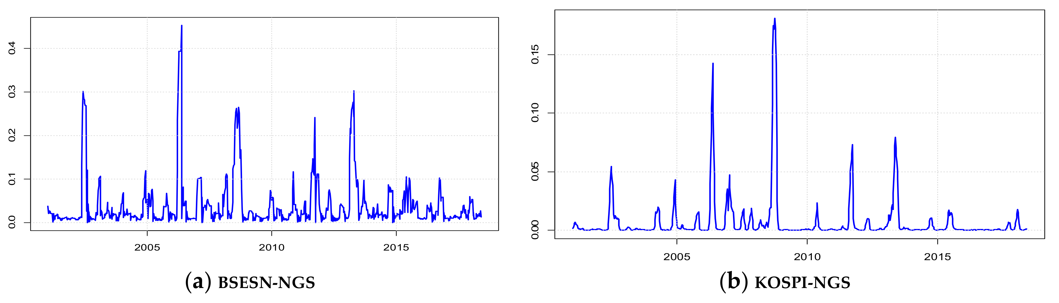
We then compute the tail dependence of these pairs to capture the dependence of extreme events in financial returns during the boom (upper tail) or market crash (lower tail) periods, as the Clayton Copula has been selected for the BSESN-NGS and KOSPI-NGS pairs and the Gumbel Copula has been selected for the BSESN-PGS, and SET-PGS pairs. The upper tail dependence is found between the Indian and Thai stock markets and positive gold shock with values of 0.06 and 0.11, respectively, for SET-PGS and BSESN-PGS. Hence, there is a higher probability of joint extreme events during the bear market than during the bull market. This is to say, the positive gold shock and Indian and Thai stock volatilities are more dependent during market downturns than during market upturns. The result also suggests strong evidence of the lower tail dependence, but the absence of the upper tail dependence in the cases of BSESN-NGS and KOSPI-NGS pairs, highlighting the importance of contagion and possibly herding during severe contractionary business cycles. According to the financial risk contagion definition, the contagion risk can be viewed as the linkage effect between financial markets caused by systemic risk and, therefore, the lower tail correlation between financial markets can be used to measure financial risk contagion [8]. The results of BSESN-NGS and KOSPI-NGS pairs point to the upper tail dependence with the values of 0.06 and 0.11, respectively. This indicates that a sharp rise or fall in Indian and Korean stock volatilities will cause a sharp rise or fall in negative gold shocks and vice versa. Additionally, the gold is likely to crash with the Indian and Korean stock markets during the market downturn, which implies that gold cannot be a safe haven in these two markets. This result is consistent with those in Section 4.2. For other pairs, there is no evidence of tail dependence; hence, joint extreme events are less likely to occur in those 16 pairs. Thus, all stock markets (except for Thailand, Korea, and India) are not significantly affected by the extreme events in the gold market in general. In other words, if positive and negative gold shocks are experienced during the extreme market upturn and downturn, respectively, then we should not expect that the shock would happen in China, India, Indonesia, Hong Kong, Philippines, Saudi Arabia, Qatar, and Vietnam simultaneously.

4.5. Measurement of Time-Varying Dependence Between Stock Volatilities and Gold Shocks

We now turn our attention to investigating the time-varying dependence structure between stock volatilities and gold shocks. In this sub-section, three Copula structures, namely the Static Copulas, Dynamic Copulas [28], and Markov Switching Dynamic Copulas [30] are considered and compared with our proposed Smooth Transition Dynamic Copulas. Again, the most appropriate model is selected while using the AIC. We noted that the explanation of the Markov Switching Dynamic Copulas is provided in Appendix A.

From the comparison results that are presented in

Table 9. AIC of three time-varying Copula models for the twenty pairs.

	SSEC	BSESN	JKSE	KOSPI	HSI	PSI	TASI	QE	SET	VNI
	STOCK-PGS
	Dynamic Copula
NORMAL	−3.158	−4.788	−3.010	−3.148	−4.789	−4.680	−2.414	−4.679	−3.279	−2.505
STUDENT-T	−1.225	−1.301	−2.315	−0.335	−0.566	−1.332	−0.115	−0.326	−2.543	−0.351
CLAYTON	−0.241	−0.541	−0.331	−0.758	−0.158	−0.9521	−1.354	−1.665	−0.554	−1.351
GUMBEL	−9.554	−4.215	−10.354	−3.012	−2.158	−6.654	−3.215	−4.941	−15.115	−2.005
FRANK	−13.845	−5.356	−15.214	−4.112	−5.331	−9.356	−4.558	−5.321	−1.358	−3.358
	Markov Switching Dynamic Copula
NORMAL	−4.525	−11.311	−5.542	−6.112	−5.348	−7.982	−3.090	−5.958	−8.213	−8.3457
STUDENT-T	−2.334	−1.566	−3.214	−0.585	−0.986	−2.912	−0.965	−0.535	−3.335	−1.661
CLAYTON	−0.456	−0.964	−0.559	−0.987	−0.542	−1.720	−2.503	−1.965	−0.983	−1.699
GUMBEL	−10.134	−13.215	−11.897	−3.985	−3.159	−7.025	−4.299	−6.001	−25.013	−6.035
FRANK	−18.812	−6.758	−15.214	−5.329	−8.883	−13.206	−8.210	−7.321	−2.118	−11.358
	Smooth Transition Dynamic Copula
NORMAL	−4.617	−10.687	−6.708	−9.114	−5.511	−7.681	−6.359	−9.329	−4.713	−6.612
STUDENT-T	−2.218	−1.516	−3.310	−0.656	−0.916	−2.609	−0.644	−0.443	−3.431	−1.203
CLAYTON	−0.994	−0.904	−0.601	−0.631	−0.593	−1.441	−2.309	−2.110	−1.022	−1.887
GUMBEL	−12.499	−12.250	−11.229	−3.914	−3.221	−7.321	−7.299	−6.591	−30.911	−5.319
FRANK	−14.114	−6.801	−18.240	−10.323	−10.305	−12.213	−8.537	−9.551	−2.389	−10.397
	STOCK-NGS
	Static Copula
NORMAL	−2.117	−9.013	−10.597	−1.817	−15.767	−11.397	1.994	2.588	−4.911	2.615
STUDENT-T	9.879	−1.809	−7.092	5.951	−10.253	−3.842	10.704	15.218	0.100	23.601
CLAYTON	15.885	−11.474	−8.442	−8.850	−11.609	−8.453	21.158	3.375	−0.829	3.972
GUMBEL	−2.300	−4.839	−8.122	−0.251	−10.030	−7.253	21.152	1.811	−3.467	2.703
FRANK	−2.836	−0.640	−0.082	2.387	−6.567	−3.135	1.722	1.519	1.228	3.097
	Dynamic Copula
NORMAL	−7.294	−6.504	−12.430	−0.149	−12.343	−16.094	−3.431	−3.896	−7.392	−6.346
STUDENT-T	−0.597	−2.115	−10.315	−1.059	−11.681	−5.361	−0.597	−0.631	−2.397	−0.398
CLAYTON	−0.158	−13.641	−10.967	−9.541	−13.189	−9.559	−0.115	−2.369	−1.117	−1.135
GUMBEL	−7.561	−4.351	−10.321	−3.987	−12.136	−8.129	−0.361	−1.336	−6.358	−1.268
FRANK	−8.054	−1.397	−1.114	−2.115	−8.669	−4.331	−5.311	−5.324	−0.554	−1.111
	Markov Switching Dynamic Copula
NORMAL	−7.285	−7.894	−13.341	−6.6413	−15.588	−14.532	−6.687	−12.300	−6.954	−9.551
STUDENT-T	−0.619	−1.995	−10.551	−1.364	−12.598	−5.368	−0.169	−0.129	−2.147	−0.188
CLAYTON	−0.264	−14.991	−11.321	−15.123	−17.597	−10.109	−0.035	−3.997	−1.006	−1.987
GUMBEL	−8.239	−5.229	−11.991	−3.558	−13.516	−9.035	−0.416	−2.691	−6.597	−1.691
FRANK	−10.065	−2.116	−1.138	−3.313	−7.024	−4.697	−7.967	−15.324	−0.597	−1.268
	Smooth Transition Dynamic Copula
GAUSSIAN	−7.783	−7.740	−14.071	−8.082	−18.358	−13.079	−6.791	−9.135	−6.076	−13.018
STUDENT-T	−0.930	−2.139	−10.202	−1.297	−14.881	−5.978	−0.221	−0.291	−2.396	−0.291
CLAYTON	−0.661	−15.169	−11.109	−15.361	−17.564	−9.119	−0.149	−3.339	−1.697	−2.068
GUMBEL	−8.321	−5.997	−12.871	−4.100	−14.336	−9.543	−0.669	−2.497	−6.570	−1.198
FRANK	−10.765	−3.156	−2.698	−3.014	−8.213	−4.793	−8.071	−15.997	−0.471	−1.303

Note: Bold number represents the lowest AIC model.

, we can find that all AIC for the MSDC and our proposed model, STDC, are lower than those for the corresponding Static Copulas for all pairs, which indicates a structural shift in the dynamic dependence structure between stock volatility and gold shock. This result confirms the Granger causality and stability tests provided in Section 4.2 and Section 4.3, respectively. Thus, this paper prefers the time-varying Copulas with regime-switching to the Static Copula for exploring the dependence structure between stock volatility and gold shock.

We then compare the performance of our STDC model with that of the MSDC model. As presented in Table 9, we find that the Markov Switching Dynamic Frank Copula (MSDC-F) is optimal for SSEC-PGS, PSI-PGS, and VNI-PGS, the Markov Switching Dynamic Gumbel Copula (MSDC-G) is optimal for BSESN-PGS, the MSDC-N is optimal for SET-NGS, the Smooth Transition Dynamic Frank Copula (STDC-F) is the optimal for JKSE-PGS, KOSPI-PGS, HSI-PGS, TASI-PGS, QE-PGS, SSEC-NGS, TASI-NGS, and QE-NGS, the Smooth Transition Dynamic Gumbel Copula (STDC-G) is optimal for SET-PGS, the Smooth Transition Clayton Copula (STDC-C) is optimal for BSESN-NGS, and KOSPI-NGS, while the Smooth Transition Dynamic Normal Copula (STDC-N) is the optimal for JKSE-NGS, PSI-NGS, HIS-NGS, and VNI-NGS. In essence, our proposed STDC model is superior to the MSDC model in 15 out of 20 pairs, according to the AIC.

Table 10. Parameter estimation for the best-fit Copula models.

	SSEC	BSESN	JKSE	KOSPI	HSI	PSI	TASI	QE	SET	VNI
	Stock-PGS
	MSDC-F	MSDC-N	STDC-F	STDC-F	STDC-F	MSDC-F	STDC-F	STDC-F	STDC-N	MSDC-F
${\omega }_{01}$	4.041 * (1.488)	2.021 * (1.001)	−0.046 * (0.001)	−0.147 * (0.056)	0.011 * (0.006)	0.388 * (0.117)	0.054 * (0.002)	−0.042 * (0.001)	−0.109 * (0.056)	3.386 * (1.506)
${\omega }_{02}$	−1.475 (1.040)	−0.697 * (0.125)	2.411 * (0.382)	5.230 * (0.549)	0.762 (0.890)	0.013 * (0.051)	1.589 * (0.537)	1.445 * (0.215)	−0.771 * (0.188)	2.825 * (1.184)
${\omega }_{03}$	−4.040 * (1.872)	−1.714 (1.419)	−0.304 * (0.009)	−4.888 (4.303)	−1.041 * (0.280)	0.107 (0.568)	1.439 (0.353)	−2.603 (1.568)	0.595 (1.125)	−0.663 * (0.391)
${\omega }_{11}$	−0.161 * (0.048)	−0.387 * (0.124)	−0.012 * (0.001)	−0.311 * (0.125)	−0.011 * (0.003	−0.465 * (0.143)	−0.154 * (0.213)	−0.154 (0.148)	0.201 * (0.021)	−0.230 0.283)
${\omega }_{12}$	1.268 * (0.496)	1.230 * (0.464)	0.140 (0.299)	−1.239 (2.287)	2.189 * (0.722)	0.082 (0.779)	−0.652 * (0.309)	−0.254 * (0.127)	0.936 * (0.331)	−0.891 * (0.031)
${\omega }_{13}$	0.308 (0.211)	0.757 (0.406)	1.333 * (0.685)	2.233 * (0.100)	2.322 * (0.302)	0.244 * (0.334)	−0.315 (0.651)	0.300 * (0.125)	−0.409 * (0.180)	0.857 (0.830)
$p_{11}$	0.867 * (0.073)	0.940 * (0.032)				0.995 * (0.004)				0.321 * (0.151)
$p_{22}$	0.974 * (0.017)	0.975 * (0.022)				0.989 * (0.007)				0.969 * (0.015)
$\gamma$			1.873 * (0.110)	2.151 * (0.067)	1.820 * (0.496)		3.114 * (1.135)	0.953 * (0.001)	0.230 (0.561)
$\mathsf{\Upsilon }$			0.427 * (0.061)	−0.525 * (0.108)	0.445 * (0.016)		0.430 * (0.074)	−0.163 * (0.035)	−0.099 * (0.001)
	Stock-NGS
	STDC-F	STDC-C	STDC-N	STDC-C	STDC-C	STDC-N	STDC-F	STDC-F	MSDC-N	STDC-N
${\omega }_{01}$	0.338 * (0.168)	0.528 * (0.204)	0.365 * (0.100)	0.037 * (0.010)	0.964 * (0.154)	0.324 * (0.125)	−0.009 * (0.004)	−0.194 (0.174)	0.573 * (0.085)	−0.051 * (0.025)
${\omega }_{02}$	−2.337 * (0.102)	−1.672 * (0.189)	−0.918 (0.994)	−0.937 * (0.554)	−2.091 * (0.100)	4.006 (4.044)	2.029 * (0.562)	1.257 * (0.328)	1.878 * (0.974)	−0.821 * (0.280)
${\omega }_{03}$	−7.677 * (0.547)	−4.515 * (2.302)	−1.941 (2.002)	−4.281 * (0.557)	−0.468 * (0.014)	0.481 (0.455)	−0.194 (1.581)	−0.310 * (0.180)	−0.490 (0.629)	−1.465 (0.861)
${\omega }_{11}$	−0.214 * (0.101)	−0.484 * (0.211)	1.090 * (0.510)	0.011 * (0.001	−0.125 * (0.054)	0.101 * (0.013)	0.103 * (0.015)	0.115 * (0.035)	−0.015 * (0.001)	0.256 * (0.100)
${\omega }_{12}$	−0.474 * (0.125)	−2.129 * (0.914)	1.001 * (0.438)	3.090 * (0.245)	−0.681 * (0.157)	−0.447 * (0.043)	1.952 (0.602)	−0.985 * (0.531)	−0.110 * (0.15)	1.361 * (0.258)
${\omega }_{13}$	2.112 * (0.554)	3.099 * (1.113)	2.994 * (1.088)	4.163 * (0.547)	−0.681 (0.611)	−2.344 * (0.103)	0.268 (1.461)	0.987 (0.540)	0.036 (0.516)	1.543 (0.683)
$p_{11}$									0.716 * (0.150)
$p_{22}$									0.938 * (0.042)
$\gamma$	0.148 * (0.003)	2.812 * (0.225)	1.786 * (0.539)	0.232 * (0.018)	0.115 (0.321)	1.006 * (0.017)	0.071 (0.280)	5.125 * (2.115)		0.086 * (0.031)
$\mathsf{\Upsilon }$	0.559 * (0.046)	−0.076 * (0.031)	0.402 (0.105)	−0.265 * (0.105)	0.493 * (0.117)	0.795 * (0.123)	0.499 * (0.125)	0.514 * (0.039)		0.349 * (0.097)

Note: (*) indicates rejection of the null hypothesis at 5% significance level. The notation “N”, “C”, “G”, and “F” represent Normal, Clayton, Gumbel, and Frank Copulas, respectively.

presents the estimated parameters with the optimal MSDC and STDC for each pair, as determined by Table 9. The parameters ${\omega }_{01}$ and ${\omega }_{11}$ represent the dependence level of regime 1 and 2, respectively. ${\omega }_{02}$ and ${\omega }_{12}$ represent the degree of persistence of regime 1 and 2, respectively; and, ${\omega }_{03}$ and ${\omega }_{13}$ capture the adjustment in the dependence process of regime 1 and 2, respectively. As shown in Table 10, the values of all parameters are mostly significant, and the values of ${\omega }_{01}$ and ${\omega }_{11}$ are quite different, which indicates that the dependency parameters do not follow the same dynamic process and there exists the structural change in the dynamic dependence. This result shows that it is reasonable to set a nonlinear or regime-switching time-varying process for the dependency structure, since the nonlinear or regime-switching time-varying dependence could better capture the relationship between the Asian emerging stock markets’ volatilities and gold shocks.

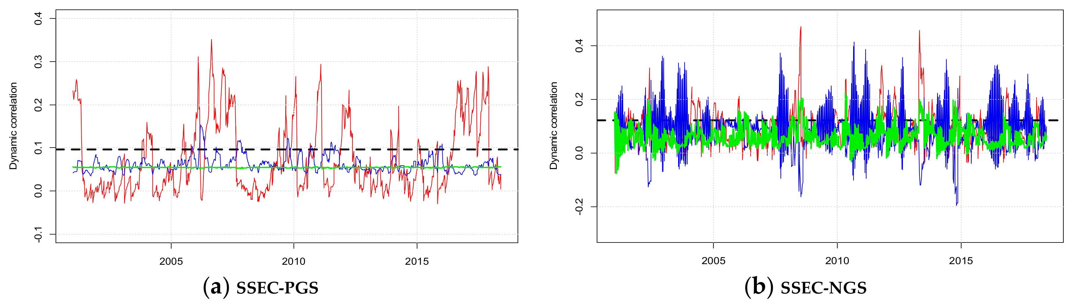
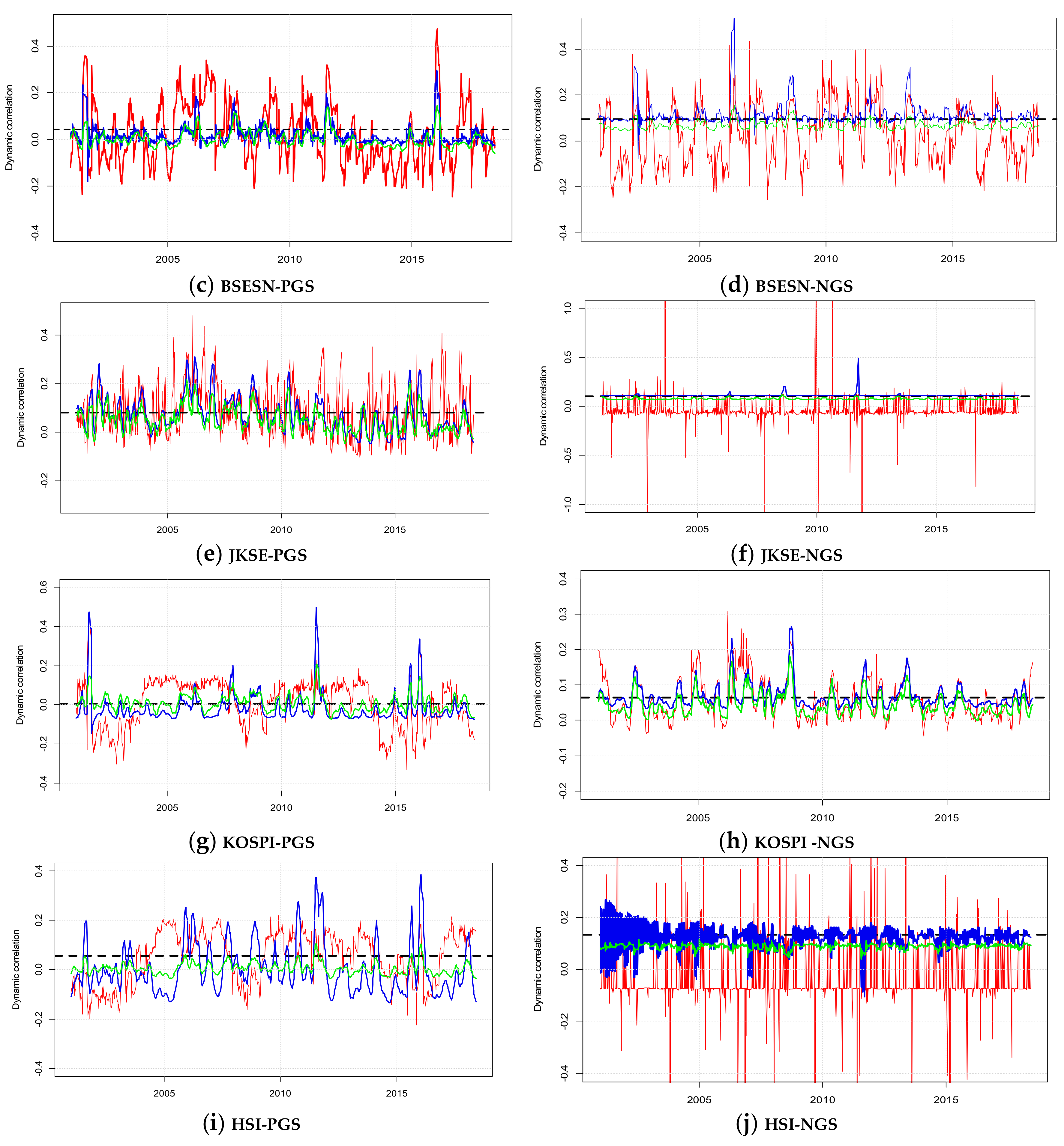
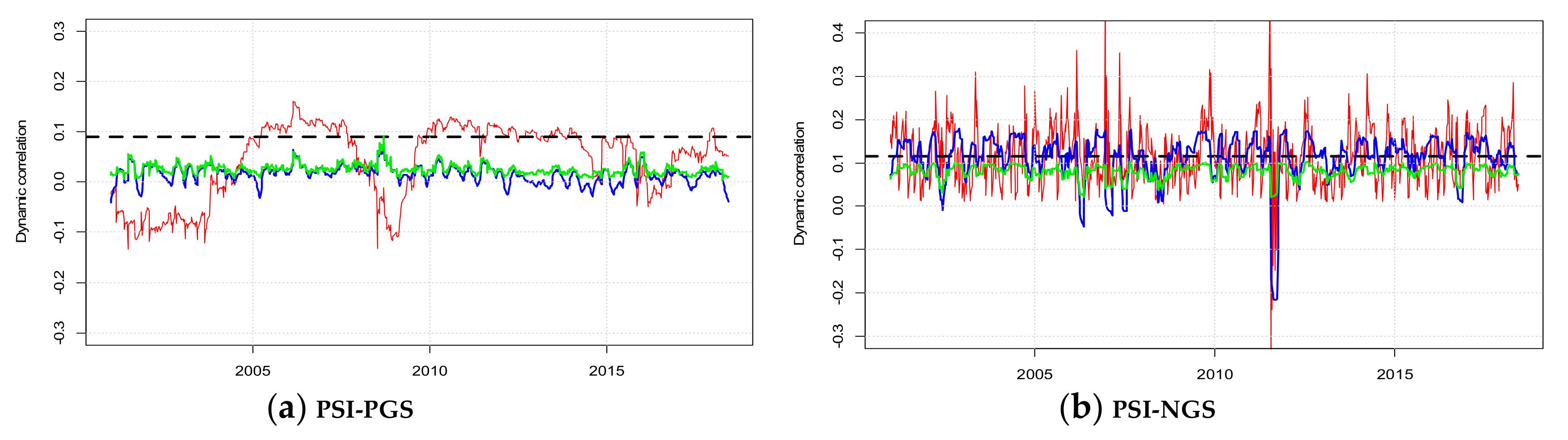
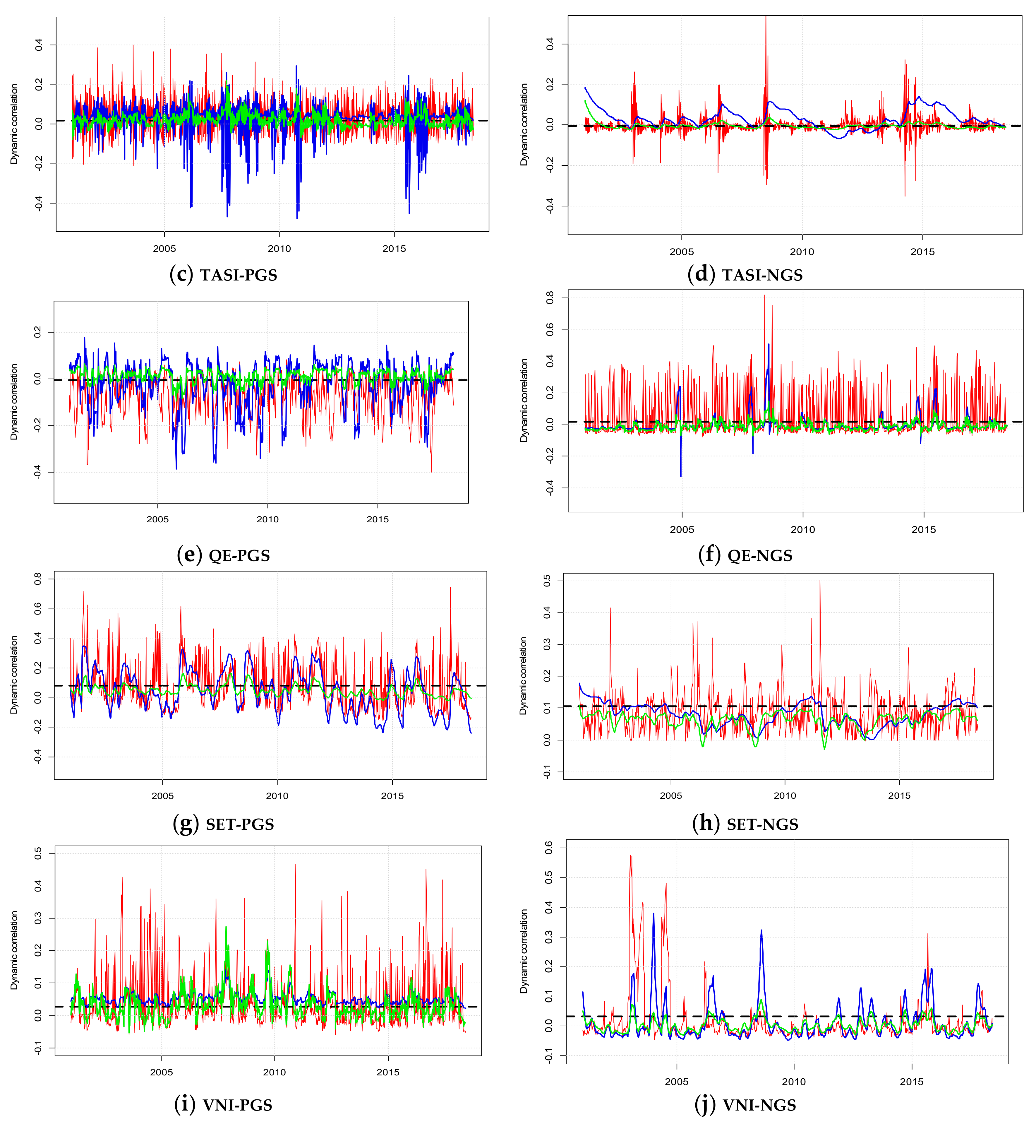
In examining the possible evolution of the dependence over time, this paper plots the time-varying Kendall’s tau estimates between the Asian emerging stock markets’ volatilities and gold shocks over the sample period generated from the best-fit model that is presented in Table 10. Figure 3 and Figure 4 plot the estimated dynamic Kendall’s from the best Static Copula (black dashed line), Dynamic Copula (green line), MSDC (red line), and STDC (blue line) for all 20 pairs. Several observations can be made and summarized, as follows. (1) The evolution of conditional Kendall’s tau values that were obtained from the four models show different time-varying paths. In general, we observe that the conditional Kendall’s tau values from MSDCs are higher and more fluctuating than those that were obtained from other copula structures, as well as our proposed model. The graphs show the biases that arise from the use of the Markov Switching Dynamic Copula model; that is, this model tends to overestimate the dependence along our sample period. (2) Among them, the SSEC-NGS pair exhibits the highest volatility pattern, whereas the time-varying dependence reaches a low of -0.2 and a high of 0.4. In contrast, the PSI-PGS pair exhibits the lowest volatility pattern, whereas the time-varying dependence ranges from -0.1 to 0.15. (3) The conditional Kendall’s tau values that were obtained from our STDC model were mostly negative and found in four cases: BSESN-PGS, KOSPI -PGS, TASI-PGS, and QE-PGS, which suggests that gold is negatively related to most of the stock markets and, thus, gold could act as a safe haven in the stock market of India, Korea, Saudi Arabia, and Qatar. (4) Regardless of the sign of the correlation obtained from the STDC model, we find that the magnitude of the correlations (blue line) of all pairs (except SET-PGS, JKSE-NGS, HSI-PGS, and HIS-NGS) is stronger during the financial crisis period (2007–2009), when compared to the normal period. In addition, it is found that the dynamic correlations of the SSEC-PGS, SSEC-NGS, BSESN-PGS, BSESN-NGS, JKSE-PGS, KOSPI -PGS, KOSPI -NGS, PSI-PGS, PSI-NGS, TASI-NGS, QE-NGS, SET-NGS, VNI-PGS, and VNI-NGS pairs are greater than zero, while those of the TASI-PGS and QE-PGS pairs are lower than 0 during the financial crisis period. This result indicates that gold can be used as an investment hedge in Saudi Arabian and Qatari stock markets, since a positive gold shock is negatively related to these two stock markets’ volatilities. However, it is instead invested just like a stock in Chinese, Indian, Indonesian, Korean, Saudi Arabian, Qatari, Thai, and Vietnamese stock markets, as a positive gold shock is positively related to these markets. Interestingly, we observe that gold can be used as hedging and non-hedging trading assets for Saudi Arabian and Qatari stock markets during the financial crisis. (5) As suggested by Xu and Gao [8], the occurrence of financial risk contagion can also be captured by the extremely positive co-movement of two financial assets. This concept is consistent with measuring the lower tail dependence between two financial assets. Thus, Clayton Copula seems to be the best choice for measuring tail dependence. However, the Clayton Copula is selected in two pairs: BSESN-NGS and KOSPI-NGS, according to the model comparison result provided in Table 10. We observe that the Indian and Korean stock markets have left tail dependence with the negative gold shock, which indicate the existence of the risk contagion effects between gold and these two stock markets. Figure 5 also confirms that financial contagion occurred during the 2007–2009 global financial crisis. The key finding of time-varying Copula dependence in three periods is shown in

Table 11. Summary results of time-varying Copula dependence in three periods.

Period	Findings
Pre-crisis	The correlations of all pairs (except VNI-NGS, VNI-PGS, BSESN-PGS, and SSEC-PGS) are quite low and close to zero. This indicates a weak dependence between stock volatilities and gold shocks.
During crisis	The magnitude of the correlations of all pairs (except SET-PGS, JKSE-NGS, HSI-PGS, and HSI NGS) is larger during the financial crisis period (2007–2009), compared to pre-crisis and post-crisis. This indicates the presence of the financial contagion effects.
Post-crisis	The correlation between stock volatility and gold shock dropped in many markets. However, it is obvious that the dependence increased again in 2015, but the magnitude is smaller compared to the financial crisis period.

.

4.6. The out-of-Sample Forecasting Performance

The out-of-sample forecasts of conditional correlation are also considered for investigating the performance and validity of our proposed STDC model. The forecasting performance of Dynamic Copula and Markov Switching Dynamic Copula models is also considered as the competitive model. In this section, the out-of-sample is demonstrated via Monte Carlo simulation for setting a one-day-ahead forecast of the conditional correlation, where the parameters are estimated each week separately based on a rolling sample with a fixed size of 104 (approximately two-year period). We use the first in-sample period starting from January 2001 to December 2002.

We use the model confidence set MCS of Hansen et al. to compare the performance of the three models [46]. The range statistic test is used, and the loss function is computed from mean squared error (MSE), which can be presented as

$$MSE=(1/N){\displaystyle \sum _{t=1}^N\left[{\left({\stackrel{⌢}{\theta }}_t-{\theta }_t\right)}^2\right]},$$

(16)

where ${\stackrel{⌢}{\theta }}_t$ and ${\theta }_t$ are the estimated conditional correlation and the realized conditional correlation, respectively. $N$ is the number of out-of-sample. It should be noted that this rolling correlation might not reflect the real value of the actual correlation, since it can only be computed from intraweek data and that the rolling correlations are computed from data spanning several months. However, the rolling correlations are still useful in observing the pattern of actual correlation.

Table 12. The out-of-sample evaluation of forecasts of correlation between positive gold shock and stock volatilities.

	SSEC	BSESN	JKSE	KOSPI	HSI	PSI	TASI	QE	SET	VNI
	STOCK-PGS
	Dynamic Copula
GAUSSIAN	0.125	0.119	0.113	0.101	0.159	0.159	0.141	0.114	0.115	0.106
STUDENT-T	0.015	0.151	0.115	0.000	0.000	0.293	0.000	0.000	0.266	0.000
CLAYTON	0.000	0.000	0.000	0.000	0.000	0.000	0.000	0.000	0.000	0.000
GUMBEL	0.123	0.151	0.135	0.169	0.221	0.111	0.109	0.309	0.133	0.159
FRANK	0.214	0.231	0.193	0.148	0.203	0.213	0.158	0.155	0.148	0.169
	Markov Switching Dynamic Copula
GAUSSIAN	0.536	0.529	0.413	0.401	0.297	0.359	0.341	0.368	0.201	0.321
STUDENT-T	0.501	0.573	0.215	0.000	0.000	0.383	0.000	0.000	0.239	0.000
CLAYTON	0.000	0.000	0.000	0.000	0.000	0.000	0.000	0.000	0.000	0.000
GUMBEL	0.524	1.000	0.335	0.269	0.357	0.329	0.329	0.448	0.359	0.233
FRANK	1.000	0.521	0.593	0.448	0.403	1.000	0.905	0.401	0.254	1.000
	Smooth transition Dynamic Copula
GAUSSIAN	0.310	0.520	0.435	0.529	0.301	0.268	0.498	0.509	0.366	0.468
STUDENT-T	0.398	0.561	0.663	0.000	0.000	0.000	0.401	0.495	0.498	0.000
CLAYTON	0.000	0.000	0.000	0.000	0.000	0.000	0.000	0.000	0.000	0.000
GUMBEL	0.418	0.997	0.544	0.331	0.359	0.297	0.551	0.697	1.000	0.559
FRANK	0.999	0.498	1.000	1.000	1.000	0.951	1.000	1.000	0.158	0.801

and

Table 13. The out-of-sample evaluation of forecasts of correlation between negative gold shock and stock volatilities.

	SSEC	BSESN	JKSE	KOSPI	HSI	PSI	TASI	QE	SET	VNI
	STOCK-NGS
	Dynamic Copula
GAUSSIAN	0.114	0.204	0.367	0.000	0.432	0.554	0.158	0.411	0.211	0.259
STUDENT-T	0.000	0.000	0.248	0.000	0.299	0.319	0.000	0.000	0.165	0.000
CLAYTON	0.000	0.594	0.298	0.413	0.331	0.334	0.000	0.059	0.035	0.321
GUMBEL	0.239	0.336	0.309	0.211	0.305	0.398	0.000	0.023	0.298	0.001
FRANK	0.331	0.307	0.059	0.198	0.106	0.301	0.254	0.498	0.000	0.002
	Markov Switching Dynamic Copula
GAUSSIAN	0.201	0.112	0.342	0.000	0.551	0.665	0.136	0.561	1.000	0.296
STUDENT-T	0.000	0.000	0.350	0.000	0.301	0.561	0.000	0.000	0.158	0.000
CLAYTON	0.000	0.631	0.348	0.539	0.359	0.595	0.000	0.000	0.005	0.447
GUMBEL	0.319	0.441	0.409	0.358	0.399	0.543	0.000	0.000	0.301	0.000
FRANK	0.564	0.403	0.010	0.201	0.111	0.299	0.413	0.579	0.000	0.000
	Smooth transition Dynamic Copula
GAUSSIAN	0.259	0.315	1.000	0.000	1.000	1.000	0.200	0.871	0.597	1.000
STUDENT-T	0.000	0.000	0.431	0.000	0.396	0.633	0.000	0.000	0.231	0.000
CLAYTON	0.000	1.000	0.514	1.000	0.637	0.648	0.000	0.000	0.118	0.588
GUMBEL	0.423	0.551	0.342	0.649	0.403	0.559	0.000	0.000	0.403	0.000
FRANK	1.000	0.498	0.058	0.587	0.200	0.290	1.000	1.000	0.000	0.000

show the MCS test results. Note that the higher the p-value indicates the more likely to reject the null hypothesis of equal predictive ability. This is to say, the higher the p-value, the better the model. For more details of the MCS test, refer to Hansen et al. [46].

The MCS test results are presented in Table 12 and Table 13. The forecasting superiority of the STDC model over the other two competing models is found for almost all pairs (except for SET-NGS, PSI-PGS, and VNI-PGS). We find that our STDC model exhibits greater forecasting accuracy, as its p-values obtained for various pairs are relatively larger when compared to other competing models. This result confirms the high performance of our proposed model for forecasting the correlation between the Asian emerging stock markets’ volatilities and gold shocks.

5. Conclusions

The causality and the dependence structure between them are worth discussing, as gold can play the role of a hedging (positive relationship) or non-hedging (negative relationship) trading asset in the stock market [47]. However, early studies on the nexus between gold and stock markets did not consider the contradicting impacts of gold price shocks. Moreover, previous literature regarding the relationships between gold and stock markets around the world falls short of adequately discussing the case of Asian emerging countries. Thus, in this study, the asymmetric dependence and causality between gold price shocks, namely positive and negative, and the Asian emerging stock markets’ volatilities are investigated. The understanding of the dependence and causality between these two markets is crucial in helping risk managers to obtain reliable dependence measures, and regulators and policymakers to design stress-testing frameworks that enhance the stability of financial institutions and financial systems as a whole.

In this study, we employ the time-varying Granger causality test and propose the Smooth Transition Dynamic Copula (STDC) model to examine the causality and dependence structure between the gold shocks and the Asian emerging stock markets’ volatilities, respectively. These methods offer the possibility of examining the contagion effect of the gold price dynamics before, during, and after the global financial crisis in 2007.

The presence of a structural change in Granger causality can be detected for all pairs, according to the causality results. The Granger causalities between the Asian emerging stock markets’ volatilities and both positive and negative gold shocks have substantially changed over the sample period for all cases. We find that the Granger causality effect of each series on the other is accepted during some parts of the sample period. Seven out of ten Asian emerging stock markets’ volatilities present the causal effect on the gold market before the global financial crisis. During the financial crisis, we can observe the bidirectional causality between stock volatility and negative gold shock in India, Korea, China, and Vietnam, which implies that gold might not serve as a safe haven for these markets. Finally, the results for the post-crisis period show significant causality running from all stock volatilities to gold shocks in some periods.

From the measurement of the dependence between stock and gold markets, according to the Static Copula result, there is evidence of positive dependence between the gold and the stock markets of the Asian emerging countries (except for Saudi Arabia). This suggests that the gold and the Asian emerging stock market indices do not provide diversification benefits along our sample period. However, more interesting results are obtained when we turn our intention to the time-varying dependence measure. Note that the STDC model is what we introduced in this study. Thus, our proposed model is compared to the three conventional Copula models, namely Static Copula, Dynamic Copula, and Markov Switching Copula, before interpreting the result. The model comparison result supports that our proposed model performs better than the conventional Copula models in 15 out of 20 cases. According to the time-varying results, the conditional Kendall’s tau values that were obtained from our STDC model present the negative values of Kendall’s tau in four pairs consisting of BSESN-PGS, KOSPI -PGS, TASI-PGS, and QE-PGS, which suggested that gold is negatively related to most of the stock markets. Therefore, gold can act as a safe haven for these markets. We also find that the correlation of some pairs is relatively stronger during the financial crisis when compared to the normal periods. Our results also show that gold can be used as an investment hedge in Saudi Arabian and Qatari stock markets as a positive gold shock is negatively related to these two stock markets’ volatilities. However, it is instead invested just like a stock in the Chinese, Indian, Indonesian, Korean, Saudi Arabian, Qatari, Thai, and Vietnamese stock markets, as the positive gold shock is positively related to the returns from these markets. Finally, there is evidence of tail dependence between Indian stock and negative gold shock and between Korean stock and negative gold shock, indicating the existence of the risk contagion effects between gold and these two stock markets.

Finally, our results show that using the time-varying Granger causality and the proposed Smooth Transition Dynamic Copula to capture causality and dependency is a useful and flexible approach. There are several opportunities for future research, such as investigating the relationship between other precious metal shocks (silver and platinum) and stock markets while using our proposed model. As the logistic transition function is adopted for constructing our model, further research might improve our model by replacing this transition function with other functions, like probit and exponential functions (see, Maneejuk, Yamaka and Sriboonchitta [48]). Finally, as the rolling window linear Granger causality test is used to investigate the causality, the further study might use the rolling window nonlinear Granger causality test and rolling window quantile causality test.

References

- Wen, X.; Cheng, H. Which is the safe haven for emerging stock markets, gold or the US dollar? Emerg. Mark. Rev. 2018, 35, 69–90. [Google Scholar] [CrossRef]
- Nguyen, C.; Bhatti, M.I.; Komorníková, M.; Komorník, J. Gold price and stock markets nexus under mixed-Copulas. Econ. Model. 2016, 58, 283–292. [Google Scholar] [CrossRef]
- Pastpipatkul, P.; Yamaka, W.; Sriboonchitta, S. Portfolio selection with stock, gold and bond in Thailand under vine Copulas functions. In International Econometric Conference of Vietnam; Springer: Cham, Switzerland, 2018; pp. 698–711. [Google Scholar]
- Do, G.; McAleer, M.; Sriboonchitta, S. Effects of international gold market on stock exchange volatility: Evidence from Asean emerging stock markets. Econ. Bull. 2009, 29, 599–610. [Google Scholar]
- Chen, K.; Wang, M. Does Gold Act as a Hedge and a Safe Haven for China’s Stock Market? Int. J. Financ. Stud. 2017, 5, 18. [Google Scholar] [CrossRef] [Green Version]
- Liao, J.; Qian, Q.; Xu, X. Whether the fluctuation of China’s financial markets have impact on global commodity prices? Phys. A Stat. Mech. Its Appl. 2018, 503, 1030–1040. [Google Scholar] [CrossRef]
- Gulzar, S.; Mujtaba Kayani, G.; Xiaofeng, H.; Ayub, U.; Rafique, A. Financial cointegration and spillover effect of global financial crisis: A study of emerging Asian financial markets. Econ. Res. Ekon. Istraživanja 2019, 32, 187–218. [Google Scholar] [CrossRef] [Green Version]
- Xu, G.; Gao, W. Financial Risk Contagion in Stock Markets: Causality and Measurement Aspects. Sustainability 2019, 11, 1402. [Google Scholar] [CrossRef] [Green Version]
- Beckmann, J.; Berger, T.; Czudaj, R. Does gold act as a hedge or a safe haven for stocks? A smooth transition approach. Econ. Model. 2015, 48, 16–24. [Google Scholar] [CrossRef] [Green Version]
- Baur, D.G.; Lucey, B.M. Is Gold a Hedge or a Safe Haven? An Analysis of Stocks, Bonds and Gold. SSRN Electron. J. 2009, 40. [Google Scholar] [CrossRef]
- Markowitz, H.M. Portfolio Selection: Efficient Diversification of Investments; John Wiley & Sons: New York, NY, USA, 1959. [Google Scholar]
- Tiwari, A.K.; Adewuyi, A.O.; Roubaud, D. Dependence between the global gold market and emerging stock markets (E7+ 1): Evidence from Granger causality using quantile and quantile-on-quantile regression methods. World Econ. 2019, 42, 2172–2214. [Google Scholar] [CrossRef]
- Mishra, P.K.; Das, J.R.; Mishra, S.K. Gold price volatility and stock market returns in India. Am. J. Sci. Res. 2010, 9, 47–55. [Google Scholar]
- Bhunia, A.; Das, A. Association between gold price and stock market returns: Empirical evidence from NSE. J. Exclus. Manag. Sci. 2012, 1, 1–7. [Google Scholar]
- Hussin, M.Y.M.; Muhammad, F.; Razak, A.A.; Tha, G.P.; Marwan, N. The link between gold price, oil price and Islamic stock market: Experience from Malaysia. J. Stud. Soc. Sci. 2013, 4, 161–182. [Google Scholar]
- Choudhry, T.; Hassan, S.S.; Shabi, S. Relationship between gold and stock markets during the global financial crisis: Evidence from nonlinear causality tests. Int. Rev. Financ. Anal. 2015, 41, 247–256. [Google Scholar] [CrossRef] [Green Version]
- Mensi, W.; Beljid, M.; Boubaker, A.; Managi, S. Correlations and volatility spillovers across commodity and stock markets: Linking energies, food, and gold. Econ. Model. 2013, 32, 15–22. [Google Scholar] [CrossRef] [Green Version]
- Hood, M.; Malik, F. Is gold the best hedge and a safe haven under changing stock market volatility? Rev. Financ. Econ. 2013, 22, 47–52. [Google Scholar] [CrossRef]
- Pearson, K., VII. Note on regression and inheritance in the case of two parents. Proc. R. Soc. Lond. 1895, 58, 240–242. [Google Scholar]
- Engle, R. Dynamic conditional correlation: A simple class of multivariate generalized autoregressive conditional heteroskedasticity models. J. Bus. Econ. Stat. 2002, 20, 339–350. [Google Scholar] [CrossRef]
- Basher, S.A.; Sadorsky, P. Hedging emerging market stock prices with oil, gold, VIX, and bonds: A comparison between DCC, ADCC and GO-GARCH. Energy Econ. 2016, 54, 235–247. [Google Scholar] [CrossRef] [Green Version]
- Sklar, M. Fonctions de repartition an dimensions et leurs marges. Publ. Inst. Statist. Univ. Paris 1959, 8, 229–231. [Google Scholar]
- Joe, H. Multivariate Models and Multivariate Dependence Concepts; CRC Press: London, UK, 1997. [Google Scholar]
- Nelsen, R.B. An Introduction to Copulas. In Springer Series in Statistics, 2nd ed.; Springer: New York, NY, USA, 2006. [Google Scholar]
- Pastpipatkul, P.; Yamaka, W.; Sriboonchitta, S. Co-Movement and Dependency between New York Stock Exchange, London Stock Exchange, Tokyo Stock Exchange, Oil Price, and Gold Price. In International Symposium on Integrated Uncertainty in Knowledge Modelling and Decision Making; Huynh, V.N., Inuiguchi, M., Demoeux, T., Eds.; Springer: Cham, Switzerland, 2015; Volume 9376. [Google Scholar]
- Pastpipatkul, P.; Yamaka, W.; Sriboonchitta, S. Analyzing Financial Risk and Co-Movement of Gold Market, and Indonesian, Philippine, and Thailand Stock Markets: Dynamic Copula with Markov-Switching. In Causal Inference in Econometrics; Huynh, V.N., Kreinovich, V., Sriboonchitta, S., Eds.; Springer: Cham, Switzerland, 2016; Volume 622. [Google Scholar]
- Beckmann, J.; Berger, T.; Czudaj, R. Tail dependence between gold and sectorial stocks in China: Perspectives for portfolio diversification. Empir. Econ. 2019, 56, 1117–1144. [Google Scholar] [CrossRef]
- Patton, A.J. Modelling asymmetric exchange rate dependence. Int. Econ. Rev. 2006, 47, 527–556. [Google Scholar] [CrossRef]
- Da Silva Filho, O.C.; Ziegelmann, F.A.; Dueker, M.J. Modeling dependence dynamics through Copulas with regime switching. Insur. Math. Econ. 2012, 50, 346–356. [Google Scholar] [CrossRef]
- Fei, F.; Fuertes, A.M.; Kalotychou, E. Dependence in credit default swap and equity markets: Dynamic Copula with Markov-switching. Int. J. Forecast. 2017, 33, 662–678. [Google Scholar] [CrossRef] [Green Version]
- Hamilton, J.D. A new approach to the economic analysis of nonstationary time series and the business cycle. Econom. J. Econom. Soc. 1989, 57, 357–384. [Google Scholar] [CrossRef]
- Maneejuk, P.; Yamaka, W.; Leeahtam, P. Modeling Nonlinear Dependence Structure Using Logistic Smooth Transition Copula Model. Available online: http://thaijmath.in.cmu.ac.th/index.php/thaijmath/article/view/3910 (accessed on 2 October 2019).
- Silvennoinen, A.; Teräsvirta, T. Modeling multivariate autoregressive conditional heteroskedasticity with the double smooth transition conditional correlation GARCH model. J. Financ. Econom. 2009, 7, 373–411. [Google Scholar] [CrossRef]
- Dornbusch, R.; Park, Y.C.; Claessens, S. Contagion: Understanding how it spreads. World Bank Res. Obs. 2000, 15, 177–197. (In English) [Google Scholar] [CrossRef] [Green Version]
- Bollerslev, T. Generalized autoregressive conditional heteroskedasticity. J. Econom. 1986, 31, 307–327. [Google Scholar] [CrossRef] [Green Version]
- Oh, D.H.; Patton, A.J. Time-varying systemic risk: Evidence from a dynamic Copula model of cds spreads. J. Bus. Econ. Stat. 2018, 36, 181–195. [Google Scholar] [CrossRef] [Green Version]
- Granger, C.W. Investigating causal relations by econometric models and cross-spectral methods. Econom. J. Econom. Soc. 1969, 37, 424–438. [Google Scholar] [CrossRef]
- Lee, K.; Ni, S.; Ratti, R.A. Oil shocks and the macroeconomy: The role of price variability. Energy J. 1995, 16, 39–56. [Google Scholar] [CrossRef] [Green Version]
- Shi, G.; Liu, X.; Zhang, X. Time-varying causality between stock and housing markets in China. Financ. Res. Lett. 2017, 22, 227–232. [Google Scholar] [CrossRef]
- Andrews, D.W.; Ploberger, W. Optimal tests when a nuisance parameter is present only under the alternative. Econom. J. Econom. Soc. 1994, 62, 1383–1414. [Google Scholar] [CrossRef]
- Nyakabawo, W.; Miller, S.M.; Balcilar, M.; Das, S.; Gupta, R. Temporal causality between house prices and output in the US: A bootstrap rolling-window approach. N. Am. J. Econ. Financ. 2015, 33, 55–73. [Google Scholar] [CrossRef] [Green Version]
- Maneejuk, P.; Yamaka, W. Predicting Contagion from the US Financial Crisis to International Stock Markets Using Dynamic Copula with Google Trends. Mathematics 2019, 7, 1032. [Google Scholar] [CrossRef] [Green Version]
- Song, Q.; Liu, J.; Sriboonchitta, S. Risk Measurement of Stock Markets in BRICS, G7, and G20: Vine Copulas versus Factor Copulas. Mathematics 2019, 7, 274. [Google Scholar] [CrossRef] [Green Version]
- Baur, D.G.; McDermott, T.K. Is gold a safe haven? International evidence. J. Bank. Financ. 2010, 34, 1886–1898. [Google Scholar] [CrossRef]
- Chan, K.F.; Treepongkaruna, S.; Brooks, R.; Gray, S. Asset market linkages: Evidence from financial, commodity and real estate assets. J. Bank. Financ. 2011, 35, 1415–1426. [Google Scholar] [CrossRef]
- Hansen, P.R.; Lunde, A.; Nason, J.M. The model confidence set. Econometrica 2011, 79, 453–497. [Google Scholar] [CrossRef] [Green Version]
- Liu, G.D.; Su, C.W. The dynamic causality between gold and silver prices in China market: A rolling window bootstrap approach. Financ. Res. Lett. 2019, 28, 101–106. [Google Scholar] [CrossRef]
- Maneejuk, P.; Yamaka, W.; Sriboonchitta, S. Does the Kuznets curve exist in Thailand? A two decades’ perspective (1993–2015). Ann. Oper. Res. 2019, 1–32. [Google Scholar] [CrossRef]
Figure 1.
Rolling window bootstrapped p-values of LR test statistic testing of 10 pairs: BSESN-PGS, SET-PGS, KOS-PGS, PSE-PGS, JKS-PGS, BSESN-NGS, SET-NGS, KOS-NGS, PSE-NGS, and JKS-NGS.
Figure 2.
Rolling window bootstrapped p-values of LR test statistic testing of 10 pairs: HSI -PGS, QE-PGS, SSE-PGS, TAD-PGS, VNI-PGS, HSI -NGS, QE -NGS, SSE-NGS, TAD-NGS, and VNI-NGS.
Figure 3.
Time-varying Copula dependence measures. The graphs in the left column plot the time-varying Kendall’s tau between stock volatility and positive gold shock, while those in the right column plot the time-varying Kendall’s tau between stock volatility and negative gold shock for SSEC, BSESN, JKSE, KOSPI, and HSI markets: The black dashed line is the Static Copula, the green line is the Dynamic Copula, the red line is the Markov Switching Dynamic Copula (MSDC), and the blue line is the Smooth Transition Dynamic Copula (STDC).
Figure 4.
Time-varying Copula dependence measures. The graphs in the left column plot the time-varying Kendall’s tau between stock volatility and positive gold shock, while those in the right column plot the time-varying Kendall’s tau between stock volatility and negative gold shock for PSI, TASI, QE, SET, and VNI markets: The black dashed line is the Static Copula, the green line is the Dynamic Copula, the red line is the MSDC, and the blue line is the STDC.
Figure 5.
The evolution of the tail dependence in the BSESN-NGS and KOSPI-NGS pairs.