Modelling Dependency Structures Produced by the Introduction of a Flipped Classroom

Abstract

Teaching processes have been changing in the lasts few decades from a traditional lecture-example-homework format to more active strategies to engage the students in the learning process. One of the most popular methodologies is the flipped classroom, where traditional structure of the course is turned over by moving out of the classroom, most basic knowledge acquisition. However, due to the workload involved in this kind of methodology, an objective analysis of the results should be carried out to assess whether the lecturer’s workload is worth the effort or not. In this paper, we compare the results obtained from two different methodologies: traditional lecturing and flipped classroom methodology, in terms of some performance indicators and an attitudinal survey, in an introductory statistics course for engineering students. Finally, we analysed the changes in the relationships among variables of interest when the traditional teaching was moved to a flipped classroom by using Bayesian networks.

1. Introduction

Student engagement is one of the most important challenges that a lecturer can face in a first-year course. The specialised literature describes the student engagement as a keystone in effective teaching and vital for learning [1]. When it comes to statistics, or any other course about mathematics, the high levels of mathematics anxiety experienced by students, termed “Statisticophobia” by Dillon [2] in 1982, have been studied [3]. Besides, when first-year students a choose group in order, depending on their highschool scores, morning shifts, more popular among the students, are filled up with the students with the highest admission grades whereas afternoon shifts receive students with the lowest ones. Traditionally, afternoon lecture shifts have to deal with less motivated, committed and prepared students than in morning groups.

In order to stimulate student’s engagement and motivation, we put into practise a different teaching methodology. One of the most studied active methodologies by educational researchers is the so-called flipped classroom or inverted classroom, which, at its most basic level, consists of reversing the learning arrangement by delivering instructional content out of class, making use of different learning material (video lectures, readings, online presentations, etc.), so that in-class time is used for discussions, formative assessments, or to apply concepts during activities. The amount of content displaced out of class is variable; for instance, lecturers can cover the introductory materials as an out-of-class activity, handling the details or more advanced content inside the classroom.

Authors agree that the most significant benefits of flipping learning are the extra time available for providing more personalised instructions to students [4] and the increase of feedback during in-class sessions [5]. Overmyer [6] points out the opportunity to utilise collaborative and inquiry-based learning. Lo et al. [7] found 61 studies revealing how inverting the class is beneficial to student learning by increasing in-class time for practice and real-time feedback. Another advantage reported is that this methodology allows students to work at their own pace [1,8], developing their autonomy and independence [9].

Finally, the published experiences reveal that students embrace this pedagogical approach with enthusiasm [10]: O’Flaherty et al. [1] found a large number of articles where surveys reported an increased student satisfaction with the flipped approach, and a meta-analysis carried out by Lo et al. [7] of 21 comparison studies showed a preference for of the flipped classroom over the traditional classroom for mathematics education. Attitudinal surveys conducted by Gilboy et al. [8] showed that a majority of students prefer watching video lectures over face-to-face lectures and that they learned the material more effectively by online recorded lectures.

Nevertheless, not everything is advantageous. Students might feel uneasy because they are not used to the inversion of traditional classroom roles [10]. Out-of-class learning seems to be the main challenge that students face when flipping the class, due to unpreparedness for this type of task [11] and the impossibility of asking questions [5]. Also, the course of the class can be hampered when students do not prepare the assigned material [12].

However, what makes flipping classroom an intimidating methodology is the heavy workload involved. Limniou et al. [9] point out that the main responsibility of the instructor is to design stimulating learning activities and material, whereas O’Flaherty [1] asserts that the content and the class activities are more important than the resources used for flipping. Others authors [4,7] note the importance of instructional videos created by the lecturer instead of using external resources. Moreover, it is advisable [7] to implement a structured formative assessment of the out-of-class learning content at the beginning of the classroom lesson in order to assess the students’ learning processes, identify misconceptions, provide daily feedback, and encourage students to study the material and to attend class.

All in all, experiences published in the literature are inspiring; however, is there a significant improvement in the students’ performance and attitude that makes flipping a classroom a worthwhile methodology? We tried to answer this question by means of analysing some performance indicators (the success rate, performance rate, percentage of students sitting the final exam and marks from the different modules of the subject), comparing their values with the same indicators when a traditional lecture was taught. Furthermore, we studied whether the introduction of the flipping classroom methodology causes a change in the dependency structures of those indicators. To carry out the dependency structure, we used Bayesian networks because this tool is extremely useful when we want to describe the dependency between variables. Their qualitative components let us identify independencies in an easy way while the quantitative component facilitates a posteriori probabilities to study varied scenarios.

2. Methodology

2.1. The Flipped Subject

The subject of this research study is an introductory course to statistics taught in four branches of the bachelor’s degree in industrial engineering (electrical engineering, industrial chemical engineering, industrial electronics engineering, and mechanical engineering) in the School of Engineering of University of Almería. The subject is held during the second semester of the first year and is supported by 45 lecture hours (31 h corresponding to theoretical lessons and 15 practice hours) and 150 self-study hours. The syllabus of the course covers topics about descriptive statistics, probability, random variables, probability distributions, and basic parametric inference.

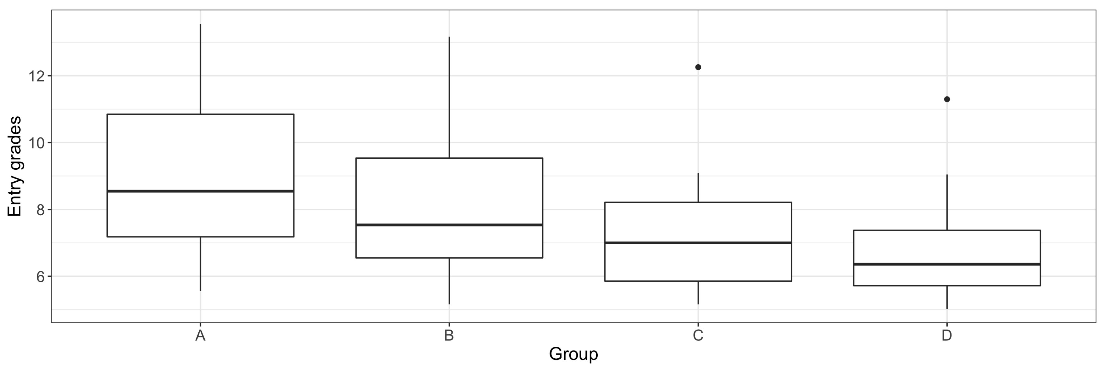
The subject is lectured in four groups (two in the morning and two in the afternoon), and students sign up for a group according to their admission grades. Figure 1 displays the difference in the student’s admission grade in the academic year 2016/2017, where groups A and B belong to the morning shift and groups C and D to the afternoon shift. Significant differences in the mean entry grade were found (p-value < 0.0001) among the four groups. The post hoc test showed significant differences (p-value < 0.05) between all groups except for pair C-D (

Table 1. Differences in mean admission grades between groups.

Group	Dunn’s p-Value
A-B	0.0102
A-C	0
A-D	0
B-C	0.0111
B-D	0.0016
C-D	0.1730

). Regarding those students repeating the year, there was no significant difference in the proportion (p-value = 0.267), the average grade (p-value = 0.496), or the number of passed credits (p-value = 0.635).

Each group had a different lecturer, and in the group where the subject was inverted (group C), two different teachers delivered the lectures (teacher 1, theoretical classes, and teacher 2, practical lessons). The traditional methodology was used in groups A, B, and D, while the new methodology was introduced in group C in 2017, which was compared with the results obtained by group C in the previous year, wherein a traditional methodology was used by the same lecturers. The students of the four groups took the same final exam and the assignments were similar in both years, each having approximately the same number, type, and difficulty of questions.

In the theoretical classes, students were given a guide about what topic they had to prepare as an out-of-class activity and two supporting materials: slides presentation made by teacher 1 and readings available online at the library of the University. The beginnings of the classroom lectures were devoted to clarifying questions, and, whenever necessary, giving a mini-lecture (10–15 min) covering details or the most difficult points. After that, a test intended to highlight and to remind students of the main points learned outside the classroom would take place. This daily assessment turned out to be very helpful in detecting and correcting students’ misconceptions and represented 10% of the students’ overall grades. The remainder of the in-class time was spent on solving textbook-type problems, some of them solved by the lecturer and others by the students in groups. While students were working in groups solving an activity, the instructor moved around the groups answering questions and guiding them towards the solution. These kinds of activities helped to increase the interactions of the students with the instructor and with their peers.

The practical lessons can be divided into two types: practical lessons devoted to solve textbook-type problems about probability and probability distributions (8 h) and practical lessons in a computer lab where students learned to use the statistical software ”Statgraphics” to solve problems about data exploratory analysis and inference (6 h). In the first-type, practical lessons, students must complete a number of homework activities independently before the class; during the practical lesson students worked in groups discussing their answers, aiming to find a common solution to every problem. These activities allow students to apply the knowledge acquired out of class to support their answers and help explain the material to their peers. In case of a disagreement, the instructor led students through the right way. At the end of the practical lesson, each group had to deliver the proposed exercises with their common solutions. To encourage the group work dynamic, the mark of those students who had not done the homework before the class was decreased 0.1 points for each unresolved exercise. In the computer lab, students solved exercises with ”Statgraphics” and answered multiple choice questions or short-answer questions individually using ”QuizSocket” (a platform no longer available, similar to “Kahoot!”) or ”Blackboard” (https://www.blackboard.com/). Performance on working groups assignments represented 20% of a student’s overall grade.

2.2. Variables under Study

We divided the study of the effect of the change in methodology on the students’ performances and attitudes into three stages. We first analysed the student’s performance by comparing the following variables:

• Success rate: fraction of students who manage to succeed in the course out of the students taking the exam.
• Performance rate: fraction of students who manage to succeed in the course out of the students matriculated in it.
• Percentage of students sitting the final exam.
• Grade received by the students in the continuous evaluation.

We also wanted to find out whether the new methodology had an effect on the partial grades; i.e., the grades per module (probability, random variable, and inference). As the weights of these modules varied in the final exam from 2016 to 2017, we could not compare both marks directly, so we used the percentage of marks received by the students out of the total marks for that module in the final exam, defined as propormathematics-08-00019tion of grade in a particular module.

In order to assess student perceptions, we carried out an anonymous survey on the students’ attitudes to the course (the complete survey is available as supplementary material). We will focus in the following questions:

• Time spent on studying the course, besides the class attendance (question 6).
• Whether the student used to prepare the out-of-class material every week (question 7).
• Students’ preferences for the teaching methodology (question 8).
• Students’ beliefs about whether they would pass the course (question 23).
• Whether each student thought that they would have learnt more with a traditional methodology in the teaching group (question 12).
• Assessment of the students regarding the methodology used in the teaching group (question 15).
• Assessment of the students regarding the methodology used in the working group (question 16).
• Perceptions of the students of the in-class formative assessment (question 19.1).

Additionally, we compared the assessments of the teachers when using each methodology.

Finally, we examined the dependency of the perform variables searching for a change in the dependency structure caused by the introduction of the new methodology. The variables that we have considered are detailed in

Table 2. Description of the variables considered in the analysis of the dependency structure.

Variable	Description
REP	Whether or not the student was retaken the course.
CALL	If the students passed the course in June call, September call, they failed or
	they did not sit the final exam.
PCE GD	Percentage of grade got in the formative assessment in the teaching group.
PCE GT	Percentage of grade got in the work group activities.
PROB	Percentage of mark got by the students in the final exam out of the total mark
	for probability exercises.
RV	Percentage of mark got by the students in the final exam out of the total mark
	for random variable and probability distribution exercises.
INF	Percentage of mark got by the students in the final exam out of the total mark
	for exercises about inference.

.

2.3. Bayesian Networks

As we reported above, one of the aims of this study was to search for a change in the dependency of performance variables when using the flipped classroom methodology. Bayesian networks [13,14] provide a helpful tool to describe the dependency structure between variables of different nature (qualitative and quantitative) because they provide a natural framework for relevance analysis besides being easily interpretable.

A Bayesian network [13,14] is a probabilistic graphical model for a set of variables $X=\{X_1,\dots ,X_n\}$, which is characterized by two elements or components:

• Qualitative component: a directed acyclic graph (DAG) consisting of one node for each variable in the model and a set of edges linking statistically dependent variables.
• Quantitative component: a conditional distribution $p\left(x_i\right|pa\left(x_i\right))$ for each variable $X_i$, $i=1,\dots ,n$ given its parents in the graph, denoted as $pa\left(X_i\right)$.

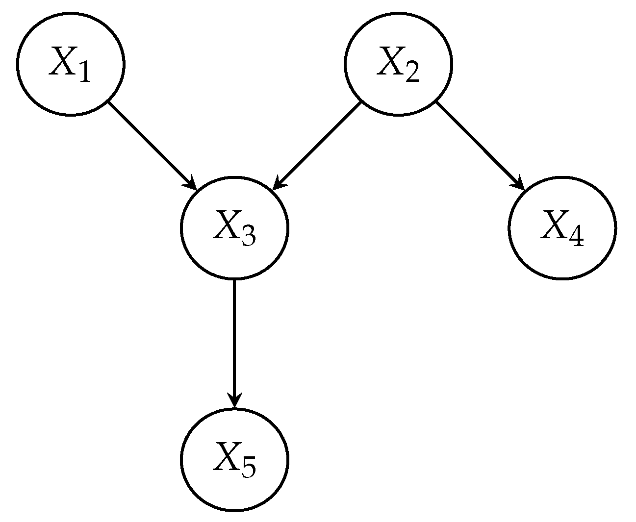
Figure 2 shows an example of the qualitative component of a Bayesian network with variables $X_1,\dots ,X_5$. The quantitative component is the distributions $p\left(x_1\right)$, $p\left(x_2\right)$, $p\left(x_3\right|x_1,x_2)$, $p\left(x_4\right|x_2)$, and $p\left(x_5\right|x_3)$.

Bayesian networks turn out to be useful tools to determine the variables that are relevant for our target variables by analysing the dependence relationships given by the structure of the DAG. More precisely, the concept of transmission of information [15] lets us carry out a relevance analysis considering two variables irrelevant to each other if the information cannot be transmitted between them.

In a DAG we can find only three types of connections among variables: serial, converging and diverging connections. We consider the Bayesian network in Figure 2 to explain the transmission of information through these three types of connections.

• Serial connections.
  • An observation on $X_1$ will influence the certainty about $X_3$ and, through this last variable, $X_1$ will also have an impact on $X_5$. Likewise, evidence on $X_5$ will influence $X_1$ through $X_3$.
  • However, if we know the value of $X_3$, the path is blocked and the evidence cannot flow from $X_1$ to $X_5$ and neither follow the contrary way.
• Diverging connections.
  • Variables $X_3$ and $X_4$ are dependent on $X_2$ and so, there is a flow of information from $X_3$ to $X_4$ or back again while no information about $X_2$ is known.
  • However if a value for variable $X_2$ is observed, the flow of information from $X_3$ to $X_4$ is stopped and evidence about $X_3$ has no effect on $X_4$.
• Converging connections.
  • Variable $X_3$ depends on both variables $X_1$ and $X_2$. But $X_1$ and $X_2$ are not related unless we have some information about $X_3$, this is, information can only be transmitted between $X_1$ and $X_2$ if we have information about $X_3$.

Summarizing, the flow of information between variables in a Bayesian network follows these rules:

• Serial and Diverging connections: Information flows between variables while the state of the middle variable is unknown.
• Converging connections: Information flows as long as information about the middle variable (or some of its descendants) is known.

We can use these rules and the structure of a Bayesian network to find out which variables have an effect on our target variables. For instance, we could determine if the grade received by a student in the formative assessment has an effect on their performance in the final exam.

Once we have set which variables can have a direct bearing on the students’performance, we would like to determine to what extent changes in those variables causes an increase or decrease in the value of the target variable.

Based on the dependences determined by the structure of the network, the joint distribution over all the variables in the network can be obtained by multiplying the conditional distribution of each node given its parents:

$$p(x_1,\dots ,x_n)=\prod _{i=1}^{n}p\left(x_i\right|pa\left(x_i\right)).$$

(1)

Let $X_i$ be our target variable and $X_E$ the variables that we have been deemed relevant for $X_i$ and that can be modified by using a new teaching methodology. Then, we can use the distribution $p\left(x_i\right|x_E)$ as a measurement of the likelihood of $X_i$ given each possible scenario of $X_E$. This probability distribution can be computed from Equation (1) or rather by using algorithms that make use of the factorisation encoded by the network structure [16,17].

3. Results

3.1. Analysis of the Students’ Performances

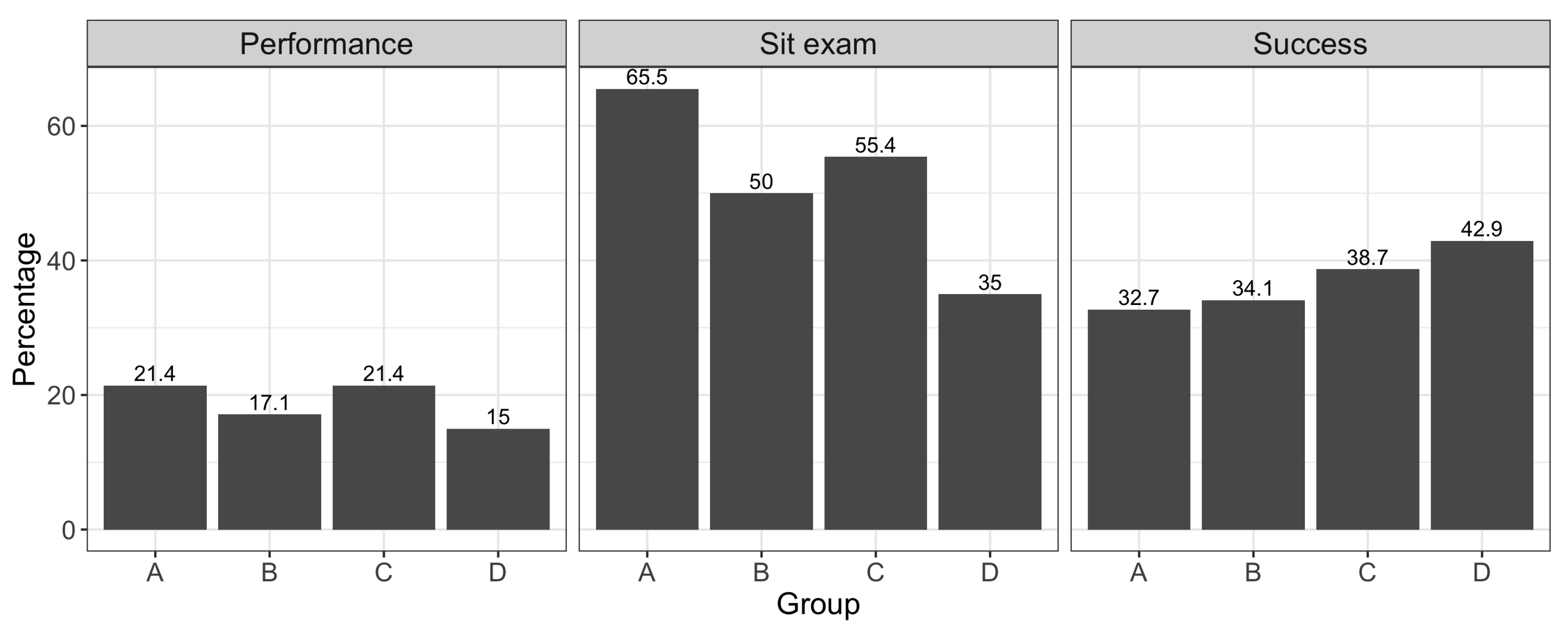
We start our analysis by comparing the success and performance rates and the percentage of students sitting the final exam among the four groups in June in 2017 (Figure 3). There were no significant differences in the three percentages among the groups (p-values from chi-square test 0.8532, 0.9562, and 0.9562 respectively).

Table 3. Comparison of the success ratio, performance ratio, and percentage of students sitting the exam by teaching group (CI for dif.: Confidence interval for the difference between the means).

Comparison	Performance Rate		Success Rate		% of Students Sitting the Exam
between Groups	p-Value	95% CI for dif.	p-Value	95% CI for dif.	p-Value	95% CI for dif.
A and C	1	(−0.1387, 0.1387)	0.7465	(−0.2966, 0.1770)	0.3040	(−0.0789, 0.2813)
B and C	0.6739	(−0.1934, 0.1063)	0.8797	(−0.2986, 0.2073)	0.6566	(−0.2379, 0.1307)
C and D	0.1500	(−0.1114, 0.24)	1	(−0.3937, 0.3108)	0.0778	(−0.0148, 0.4220)

displays p-values and 95% confidence intervals for the difference of the rates between group C and the three other groups.

Nevertheless, we cannot draw any conclusions about the performances of the students depending on the methodology used, because the difference in a student’s performance may depend on the particular instructor. So we went on comparing the results with the previous year, when the same instructors used the traditional methodology.

Table 4. Comparison of the success ratio, performance ratio, and percentage of students sitting the exam by teaching group (CI for dif.: Confidence interval for the difference between the means).

Rate	Value in 2016	Value in 2017	p-Value	95% CI for dif.
Performance	0.18	0.21	0.8040	(−0.2065, 0.1309)
Success	0.27	0.39	0.4793	(−0.3748, 0.1460)
% sitting exam	0.65	0.55	0.4308	(−0.11, 0.297)

shows the comparison between group C in 2016 and in 2017. We could not find evidence of significant differences in performance rate, success rate, or the percentage of students sitting the final exam in June depending on whether the methodology was traditional or flipped classroom.

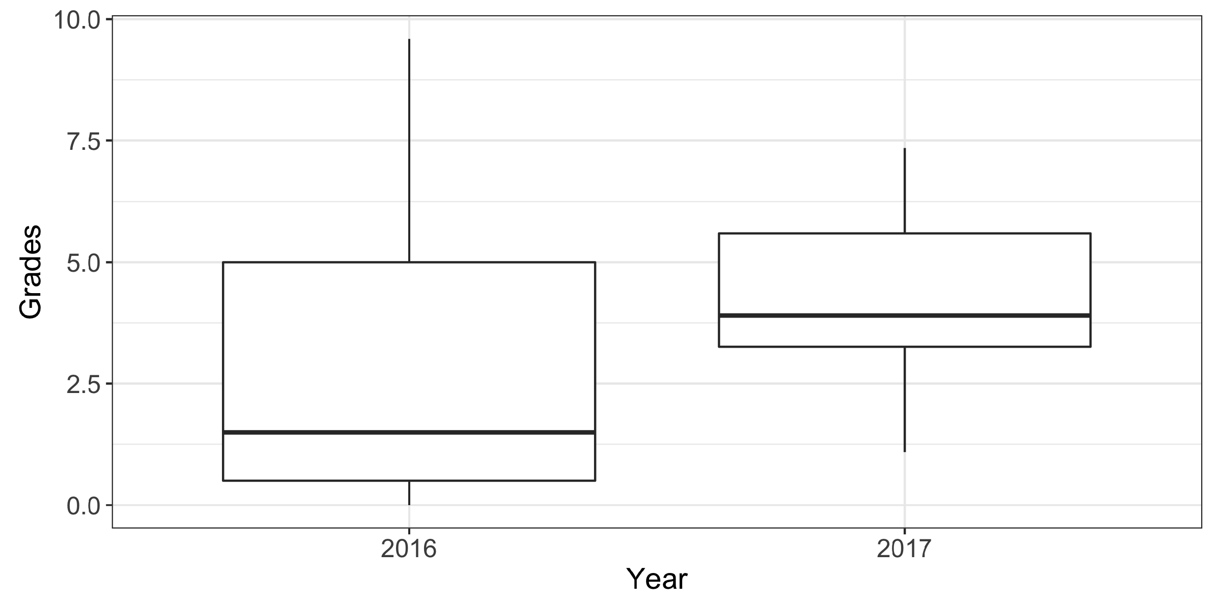
However, if we analyse the students’ grades, we observe that they were significantly higher when using the flipped classroom methodology. Not only were grades different (p-value = 0.003), but the mean grade increased 64.13%, while the median grade did by 160%, as shown in

Table 5. Comparison of the grades in years 2016 and 2017 (N: sample size; SD: standard deviation; CV: coefficient of variation).

	2016	2017
N	33	31
Min.	0	1.09
Max.	9.6	7.35
Mean	2.63	4.32
Median	1.50	3.9
SD	2.63	1.51
CV	1	0.35

. Additionally, variability in grades from the flipped classroom decreased from 1 to 0.35. Figure 4 shows the improvement in grades when the inverted classroom is used.

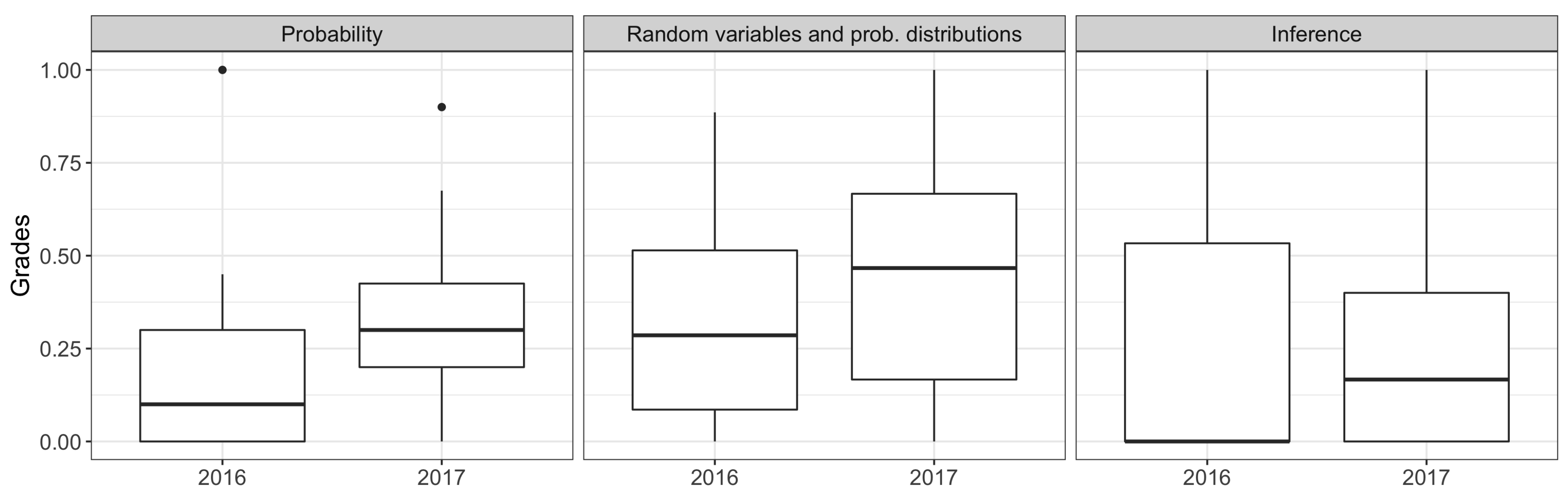
To find out whether the new methodology had an effect on the partial grades, i.e., the grades per module (probability, random variable, and inference), we considered the percentage of marks received by the students out of the total marks for that module in the final exam. We found that there were significant differences in the distributions of those grades in the modules probability and random variables (p-values less than 0.0001 and 0.046), whereas there was no significant difference in the module about inference (p-value = 0.436). In the case of module probability, the mean proportion of grade got increased from 17.2% in 2016 to 33.15% in 2017. In the exercises about random variables and probability distributions, the mean rate of grade received by the students was 29.61%, going up to 44.09% in 2017. Figure 5 illustrates this situation.

Finally, if we focus our attention on the grade received in the continuous evaluation during in-class activities, we do not find significant differences between the two years (p-value = 0.261). Despite the fact that the percentage of the students who followed the continuous evaluation along the course decreased from 80.4% in 2016 to 71.4% in 2017, the difference between both percentages cannot be considered significant (p-value = 0.393).

3.2. Analysis of Student Attitudes

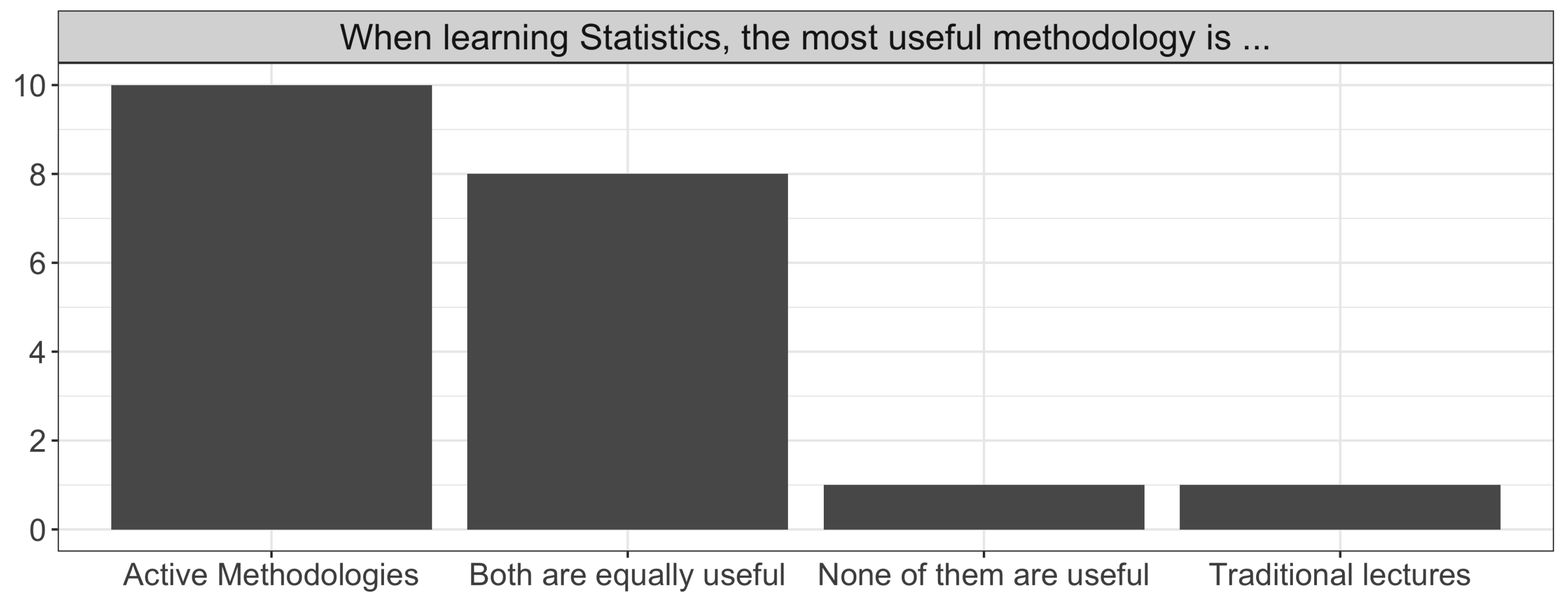
Survey responses indicates that almost two thirds of students declared spending between 2 and 3 h per week studying the subject and 60% of the students answered that they used to prepare the out-of-class material regularly. Neither preparing the out-of-class materials regularly nor time spent on doing it had an effect on the students’ preferences for the teaching methodology (p-values 0.329 and 0.872): 50% of the students preferred active methodologies to a traditional lecture format, whereas 40% of them found both methodologies equally useful (Figure 6); and just 5% of the students leant towards traditional lectures. The students’ beliefs about whether they would pass the subject did not have an effect on their preferred methodology either.

When students were asked about whether they would have learnt more with traditional teaching, preparing the out-of-class material, time spent weekly on the subject, and their beliefs about their performance in the subject, all had no effects on the answer, since 85% of the students strongly agreed or disagreed with that claim. It is remarkable to notice that no student considered that they could have learned more with a traditional lecture.

The assessment of the students about the methodology used in the teaching group was independent of their rating about the work group methodology (p-value = 0.687), with the mean rate in the teaching group being 4.25 (SD = 0.85) and 3.75 in the work group (SD = 1.29), out of five points. So we can conclude that the inverted class was highly appreciated by the students.

Regarding the in-class formative assessment, 70% of students stated that this activity had encouraged them to make a greater effort to study, regardless of whether the student prepared the material frequently and the time spent on it.

Finally, we compared the assessment of both teachers by the students. In 2016, when the traditional approach was used, teacher 1 (theoretical lessons) got a mean grade of 4.73 points out of five, with a standard deviation of 0.39, whereas the mean grade of teacher 2 (practical lessons) was 4.47 with a standard deviation of 0.5. In 2017, when the flipped the classroom methodology was applied, the means were 4.37 and 4.2 respectively, with standard deviations 0.52 and 0.72. However, these downturns in the assessment are not significant (p-value = 0.3613 and 0.3921, respectively), nor are the increases in the variability (p-value = 0.9283 and 0.4275). Hence, the change in the methodology did not have any effect on the evaluation of either instructor.

3.3. Analysis of the Dependency between Variables

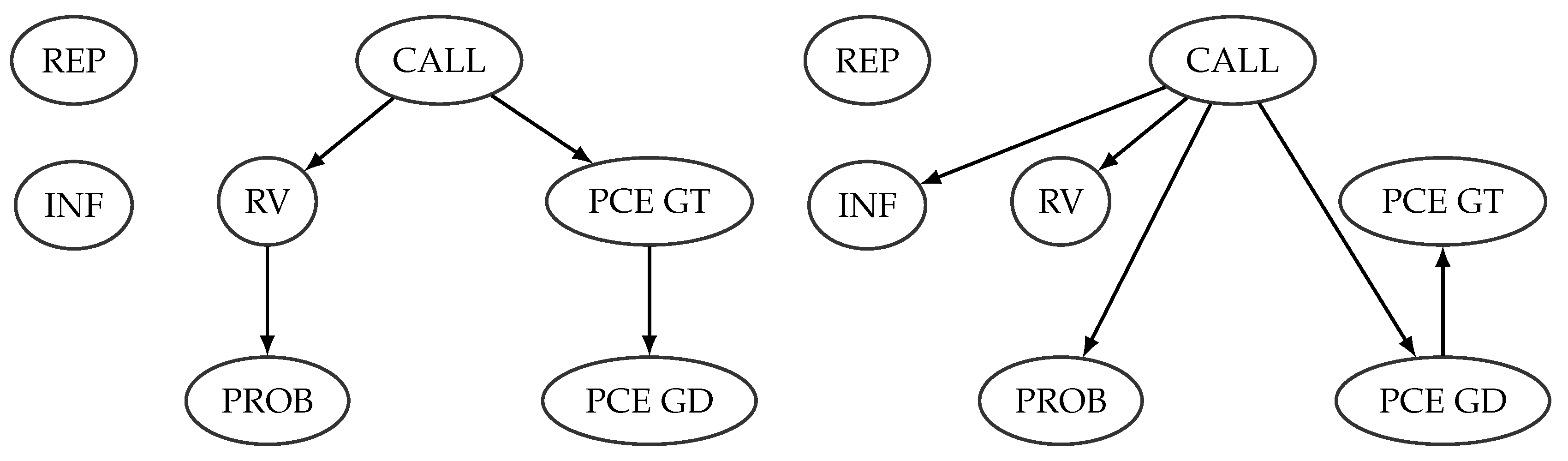
Figure 7 depicts the networks built by using the hill climbing algorithm (for explanation of the variables, see Table 2). Attending to the structure of the network in that figure, it can be seen that the fact of retaking the course does not have any implications on the students’ performances in the course independently of the methodology used. Also, in both methodologies the final result (CALL) of students in the course (either passing in June, passing in September, failing or not sitting the exam) has a direct effect on the scores received by students in the continuous evaluation (PCE GD and PCE GT). However, while the rate received in the inference module (INF) is independent of the rest of variables when traditional lectures is used, this rate is related to the rates gotten in the probability and random variable modules (PROB and RV) and the scores in the continuous evaluation throughout the variable CALL when we introduced flipped classroom. We can evaluate the effect on variable INF using the conditional probabilities displayed in

Table 6. Conditional probabilities of variable inference module (INF) given CALL using flipped classroom.

Inference	Probability	Conditional Probabilities in 2017 Given CALL
Module	in 2016	June	September	Not Pass
$[0,0^{\prime }25)$	0.75	0.18	1	0.67
$[0^{\prime }25,0^{\prime }50)$	0.08	0.36	0	0.13
$[0^{\prime }50,0^{\prime }75)$	0.14	0.18	0	0.2
$[0^{\prime }75,1]$	0.04	0.27	0	0

. Whereas in 2016 with traditional lectures, the most likely score in inference was lower than 25% of the total module-score, in 2017, with the flipped classroom, the score in inference depended on the call where the students passed the course: the most probable score among students passing in June was in the range between 25% and 50%, whereas if the student failed this exam, their most probable score was under 25%. Besides that, we can use the probabilities in the Bayesian networks to study how by changing the variable INF, we can modify the probabilities of passing the subject in June.

Another change happened in the percentage of score gotten in the probability module (PROB). When traditional lectures were used, this score depended directly on the score got in the random variables module (RV) but when we used flipped classroom, the probability module score depended on the call in which the student passed the subject (June or September), so that information flows from RV to PROB through CALL. However, if the value of CALL (June, September or not pass) is known, RV and PROB are independent.

If we focus our interest in the variable CALL with the aim to maximise the probability of passing the course in June, we can use the quantitative part of the Bayesian network to identify which actions cause the best improvement in the percentage of students passing the course in June. When a flipped classroom is used in the course, rates in the three contents are relevant to the variable CALL.

Table 7. Conditional probabilities of variable CALL given the probability module (PROB) using a flipped classroom.

CALL	Prior	PROB
	Probability	[0,0’25)	[0’25,0’50)	[0’50,0’75)	[0’75,1]
June	0.20	0	0.55	0.80	1
September	0.02	0	0	0.20	0
Not pass	0.78	1	0.45	0	0

,

Table 8. Conditional probabilities of variable CALL given the random variables module (RV) using flipped classroom.

CALL	Prior	RV
	Probability	[0,0’25)	[0’25,0’50)	[0’50,0’75)	[0’75,1]
June	0.20	0	0.29	0.80	1
September	0.02	0	0.14	0	0
Not pass	0.78	1	0.57	0.20	0

and

Table 9. Conditional probabilities of variable CALL given INF using flipped classroom.

CALL	Prior	INF
	Probability	[0,0’25)	[0’25,0’50)	[0’50,0’75)	[0’75,1]
June	0.20	0.05	0.67	0.33	1
September	0.02	0	0	0.17	0
Not pass	0.78	0.95	0.33	0.50	0

show how a good understanding of probability and random variables are essential to passing the subject. If we compute the probability of passing the course in June given two variables, the best improvement using a score as low as possible is getting between 25% and 50% in probability (PROB) and inference (INF), causing a probability of passing in June of 0.77.

With a traditional methodology there is little scope, since scores in inference (INF) are irrelevant to CALL, and scores in probability (PROB) become also irrelevant to our target variable if rates in random variables (RV) are known.

Table 10. Conditional probabilities of variable CALL given RV using a traditional methodology.

CALL	Prior	RV
	Probability	[0,0’25)	[0’25,0’50)	[0’50,0’75)	[0’75,1]
June	0.18	0	0.17	0.64	0.20
September	0.25	0.07	0.50	0.36	0.80
Not pass	0.57	0.93	0.33	0	0

shows conditional probabilities of variable CALL given the scores in random variable and probability distribution module (RV). Students should get between 50% to 75% of the total mark in this module to increase the probability of passing the subject in June from 0.18 to 0.64. Disregarding variable RV, a little improvement in the score of probability (between 25% and 50% of the total mark in probability) makes a difference by increasing the probability of passing the course in June by 30 points (

Table 11. Conditional probabilities of variable CALL given PROB using a traditional methodology.

CALL	Prior	PROB
	Probability	[0,0’25)	[0’25,0’50)	[0’50,0’75)	[0’75,1]
June	0.18	0.07	0.48	0.27	0.34
September	0.25	0.13	0.34	0.53	0.60
Not pass	0.57	0.80	0.18	0.20	0.06

).

4. Discussion

Facing the question about whether introducing a flipped classroom methodology is worth the lecturer’s workload increase, the most objective answer, in view of the results obtained, is that it depends on the aim pursued. The analysis of the students’ results shows that not the success ratio, the performance ratio, nor the percentage of students sitting the final exam, are improved by flipping the class. Furthermore, the assessment of the instructors by their students seems to remain unchanged when the new methodology is used. However other authors, such as McBride [4], obtained higher pass rates after using this new format in their classes. The use of videos made by the instructor or recorded classes are advised and can make a difference in the students’ results when this methodology is used.

On the other hand, the improvement in the students’ grades is significant; particularly, the median is highly increased and the variability in the grades reduced. This achievement might be an incentive itself to implement the methodology. Nevertheless, we have to take into consideration the limitations of the study. The student profile can be different from one year to another; however, it was expected that this difference was not significant given that students belonged to two consecutive years and the admission conditions and degrees were the same. In 2017, we cannot compare the results of our group with the other groups (where the traditional methodology was used), because the lecturers are different, and that might bias the results. In order to study possible significant differences between both morning and afternoon shifts in the students’ performances, and, if so, whether these differences disappear when the flipped classroom methodology is used, both groups must have the same lecturer.

Regarding the students’ attitudes, they show a preference for active methodologies, although a similar percentage of respondents think that both traditional lectures and an inverted classroom are equally useful in their learning. Again, it would be interesting to analyse whether morning shift groups report the same preferences.

Finally, the change in the dependency of the variables when a flipped classroom is used offers more room for manoeuvring when we try to improve the performance in the final exam. For example, we can try to get a higher passing rate in June by emphasising the students’ understanding of random variables or inference, as our results highlight.

To conclude, possible future studies could involve the comparison of the effect of flipped classroom on groups with more engaged and prepared students (in our case students from morning shifts) or the analysis of how the use of videos (or recorded classes) affect the students’ performances when using the flipped classroom methodology.

References

- O’Flaherty, J.; Philiphs, C. The use of flipped classrooms in higher education: A scoping review. Internet High. Educ. 2015, 25, 85–95. [Google Scholar] [CrossRef]
- Dillon, K. Statisticophobia. Teach. Psychol. 1982, 9, 117. [Google Scholar] [CrossRef]
- Philiphs, L.; Phillips, M. Improved student outcomes in a flipped statistics course. Adm. Issues J. 2016, 6, 88–98. [Google Scholar]
- McBride, C. Flipping Advice for Beginners: What I Learned Flipping Undergraduate Mathematics and Statistics Classes. PRIMUS 2015, 25, 694–712. [Google Scholar] [CrossRef]
- Guerrero, S.; Beal, M.; Lamb, C.; Sonderegger, D.; Baumgartel, D. Flipping Undergraduate Finite Mathematics: Findings and Implications. PRIMUS 2015, 25, 814–832. [Google Scholar] [CrossRef]
- Overmyer, J. Research on Flipping College Algebra: Lessons Learned and Practical Advice for Flipping Multiple Sections. PRIMUS 2015, 25, 792–802. [Google Scholar] [CrossRef]
- Lo, C.W.; Hew, K.F.; Chen, G. Toward a set of design principles for mathematics flipped classrooms: A synthesis of research in mathematics education. Educ. Res. Rev. 2017, 22, 50–73. [Google Scholar] [CrossRef]
- Gilboy, M.B.; Heinerichs, S.; Pazzaglia, G. Enhancing Student Engagement Using the Flipped Classroom. J. Nutr. Educ. Behav. 2015, 47, 109–114. [Google Scholar] [CrossRef] [PubMed]
- Limniou, M.; Schermbrucker, I.; Lyons, M. Traditional and flipped classroom approaches delivered by two different teachers: The student perspective. Educ. Inf. Technol. 2018, 23, 797–817. [Google Scholar] [CrossRef] [Green Version]
- Strayer, J.F. How learning in an inverted classroom influences cooperation, innovation and task orientation. Learn. Environ. Res. 2012, 15, 171–193. [Google Scholar] [CrossRef]
- Kraut, L. Inverting an Introductory Statistics Classroom. PRIMUS 2015, 25, 683–693. [Google Scholar] [CrossRef]
- Wilson, S.G. The Flipped Class: A Method to Address the Challenges of an Undergraduate Statistics Course. Teach. Psychol. 2013, 40, 193–199. [Google Scholar] [CrossRef]
- Castillo, E.; Gutiérrez, J.; Hadi, A. Expert Systems and Probabilistic Network Models; Springer: New York, NY, USA, 1997. [Google Scholar]
- Jensen, F.V.; Nielsen, T.D. Bayesian Networks and Decision Graphs; Springer: New York, NY, USA, 2007. [Google Scholar]
- Fernández, A.; Morales, M.; Rodríguez, C.; Salmerón, A. A system for relevance analysis of performance indicators in higher education using Bayesian networks. Knowl. Inf. Syst. 2011, 27, 327–344. [Google Scholar] [CrossRef]
- Madsen, A.L.; Jensen, F.V. Lazy propagation: A junction tree inference algorithm based on lazy evaluation. Artif. Intell. 1999, 113, 203–245. [Google Scholar] [CrossRef] [Green Version]
- Shenoy, P.P.; Shafer, G. Axioms for probability and belief function propagation. In Uncertainty in Artificial Intelligence 4; Shachter, R., Levitt, T., Lemmer, J., Kanal, L., Eds.; Springer: Amsterdam, The Netherlands, 1990; pp. 169–198. [Google Scholar]
Figure 1.
Admission grades depending on the shift: morning (A and B) or afternoon (C and D).
Figure 2.
An example of a Bayesian network with five variables.
Figure 3.
Percentages of success, performance, and students sitting the final exam per group.
Figure 4.
Box plot of grades in 2016 and 2017.
Figure 5.
Grades obtained over possible grade by learning module.
Figure 6.
Students’ opinions about their preferences in teaching methodology.
Figure 7.
(a) Traditional methodology. (b) Flipped classroom methodology.