Reverse Mortgage Risks. Time Evolution of VaR in Lump-Sum Solutions


Facultad de Ciencias Económicas y Empresariales, Universidad de Alcalá. Plaza de la Victoria, 2, Alcalá de Henares, 28802 Madrid, Spain
*
Author to whom correspondence should be addressed.
†
These authors contributed equally to this work.
Mathematics 2020, 8(11), 2043; https://0-doi-org.brum.beds.ac.uk/10.3390/math8112043
Submission received: 28 October 2020
/
Revised: 8 November 2020
/
Accepted: 10 November 2020
/
Published: 17 November 2020
(This article belongs to the Special Issue Application of Mathematical Analysis and Models to Financial Economics)
Abstract
:In this study, we analyzed the risk faced by the reverse mortgage provider in the case of the lump-sum solution, which is increasingly becoming one of the most popular types of reverse mortgages. The risk faced by the mortgage provider was estimated by means of a value at risk (VaR) procedure that involves a Monte Carlo simulation method and an ARMA-EGARCH assumption for modeling house price returns in the United Kingdom from 1952 to 2019. The results showed that the reverse mortgage provider faced higher risk and consequently needed to allocate more funds to meet its regulatory capital requirements in the case of relatively young borrowers, especially when they reached their life expectancy and had high roll-up rates. The risk was even higher in the case of the female population. Furthermore, care must be taken when the rental yield rate is higher than the risk-free rate, as is currently the case, as the value of the no-negative-equity guarantee (NNEG) is relatively high and results in higher value at risk (VaR) and expected shortfall (ES) values. These results have important implications in terms of policy decision making when determining the countercyclical buffer for reverse mortgages in Basel III, as well as from a managerial perspective when determining the economic capital needed to support the risk taken by the lender.
1. Introduction
Reverse mortgages are granted by banks to elderly people who want to supplement their incomes, with the borrower’s home as collateral. The borrower receives an amount of money, in the form of either a lump sum or periodic payments, and when he/she dies or moves out of the house, the amount of the home sale is used to repay the loan (plus interest). Moreover, in a majority of cases, a no-negative-equity guarantee (NNEG) is incorporated into the loan. This is done so that at the time of death or abandonment of his/her home, the borrower is only responsible for the sale price of his/her home, which represents a potential loss for the mortgage provider. The NNEG could be interpreted as a European put option that could be exercised by the borrower at the time of his/her death.
From a risk management perspective, reverse mortgages are complex products because they involve several types of risks—longevity risk, house price risk, interest rate risk, and rental yield risk. This study analyzed the risk faced by the reverse mortgage provider over time. This risk was quantified in terms of the value at risk (VaR) and the expected shortfall (ES), according to the Basel III regulations.
The proposed method for calculating the VaR and the ES is based on the [1] method for estimating the NNEG, which involves estimating an ARMA-EGARCH model for house price returns and Monte Carlo simulation techniques. Based on this method, we estimated the value of a theoretical portfolio of reverse mortgages owned by a financial institution, and we analyzed how this portfolio value varied as the borrower became older, taking into account both the house price risk and longevity risk (by means of the model in [2]). Using this procedure, we estimated a one-year VaR and ES every year, which allowed us to analyze how the reverse mortgage provider’s risk varied over time.
1.1. Literature Review
There is extant literature on the valuation of reverse mortgages, taking into account different types of risks. Within this line of research, [1] proposed an ARMA-EGARCH process for house prices to value the NNEG in lump-sum reserve mortgages using data from the United Kingdom, allowing for stochastic mortality rates according to [2]. The approach by [1] was extended by [3] to the valuation of the nonrecourse provision of reverse mortgages in the United States, allowing for stochastic mortality rates with asymmetric jump effects. Later, [4] incorporated interest rate risk into the analysis, and [5] incorporated the relationship between house prices and some key macroeconomic variables. A Vector Autoregressive (VAR) model for jointly modeling house price risk, interest rate risk and rental yield risk was proposed by [6], while [7] proposed a Bayesian method for valuing reverse mortgages involving house price risk, interest rate risk, and mortality risk. The combined effect of stochastic house prices and interest rates on the valuation of reverse mortgages was analyzed by [8]. Idiosyncratic house price risk and longevity risk were incorporated into the analysis by [9,10], allowing for stochastic interest rates and variable mortgage roll-up rates.
More recently, [11] proposed using neural networks to project real estate market data to obtain a dynamic pricing algorithm for reverse mortgages. Ref. [12] proposed a product similar to the reverse mortgage, which consisted of a contractual scheme where an immediate life annuity was obtained in exchange for transferring the property of the house to an insurer while keeping the usufruct.
Despite the extensive literature on reverse mortgage valuation, the literature on calculating regulatory capital requirements for these types of products is still scarce. A procedure for estimating the severity of losses to the reverse mortgage provider was proposed by [13], using a VAR model for house prices, interest rates, and Consumer Price Index (CPI) in the Australian market. However, these authors did not value the NNEG. More recently, [14] analyzed the risk and profitability of reverse mortgages from the mortgage provider point of view using a valuation model that allowed for house price risk, interest rate risk, and risk of delayed loan termination. They found that lump-sum reverse mortgages were more profitable and required less risk-based capital than income-stream reverse mortgages. Ref. [6] used the same procedure as [14] for comparing the risk faced by the lender in reverse mortgages and home reversion contracts, finding that reverse mortgages delivered less risk to the provider than home reversions. However, both studies [6,14] estimated a VAR model for jointly modeling house prices, interest rates, and rental yields without considering the heteroskedasticity effect commonly observed in house prices (see [1]) and assumed a Gompertz structure for the population force of mortality. Both studies also provided estimations of the VaR and ES, from the lender’s perspective, for a reverse mortgage (or home reversion contract) granted to a single person.
1.2. Our Contribution
In the present study, we addressed these drawbacks by (i) proposing an ARMA-EGARCH model allowing for heteroskedasticity in house prices; (ii) taking into account longevity risk using the model described in [2]; and (iii) providing a procedure for calculating the regulatory capital requirements for the reverse mortgage provider by considering a theoretical portfolio of reverse mortgages (instead of a reverse mortgage granted to a single person) and assuming that the number of deaths followed a binomial distribution. Table 1 summarizes the main advantages and drawbacks of the existing studies, addressing the problem of calculating the regulatory capital requirements for reverse mortgages, compared to those of the present study.
Moreover, to the best of our knowledge, this is the first time a dynamic analysis of the risk faced by the reverse mortgage provider has been addressed, and this issue has important implications in terms of the regulatory capital requirements for financial institutions according to Basel III regulations.
Specifically, in this paper, we analyzed the risk faced by the reverse mortgage provider as time passes, in the case of the lump-sum solution, which is the product design that dominates in most markets today. This risk is quantified in terms of the VaR and the ES according to the Basel III regulations.
The empirical application is performed using data from the United Kingdom from 1952 to 2019. The results showed that the reverse mortgage provider must allocate higher amounts of funds to meet its legal capital requirements for relatively young borrowers, especially when they reach their life expectancy and in cases of high roll-up rates. We also provided evidence of higher risk in the female population and when the rental yield rate is higher than the risk-free rate, as is currently the case. This fact has important implications in policy decision-making, as the cyclicality of reverse mortgage providers’ earnings induced by variations in rental yields must be taken into account by the authorities when determining the countercyclical buffer in Basel III. Moreover, from a managerial perspective, the lender should take into account that reverse mortgages granted to relatively young borrowers assume that the amount of economic capital needed to support the risk taken will rise as the borrower gets older. This risk will reach a peak around his/her life expectancy, with the amount being higher for female borrowers and for high roll-up rates.
It is worth noting that our main goal is to provide a method for analyzing the time evolution of the risk faced by the reverse mortgage provider over time and, therefore, to provide a relatively simple and tractable method to estimate the time evolution of the capital requirements for these products in accordance with Basel II and III. In this sense, it must be highlighted that our approach has two main drawbacks. The first is that our method does not allow for stochastic interest rates. The second is that, contrary to [14], we do not consider the probability of reverse mortgage loan termination due to long-term care moveout, prepayment, and refinancing. We must take into account that our method considers three different sources of risk: house price risk, longevity risk, and the risk associated with the number of survivors in the theoretical portfolio of reverse mortgages owned by the financial institution.
1.3. Paper Roadmap
The rest of the paper is organized as follows. Section 2 describes the house price, mortality, interest rate, and rental yield data used in the study. The ARMA-EGARCH model for house price returns is described in Section 3. The method for estimating the NNEG and the methods for calculating the VaR and the ES are contained in Section 4. The results are presented in Section 5. Finally, Section 6 contains the main conclusions of the paper.
2. Data
Given that the value of reverse mortgages is affected by several risk sources, our database is composed of different series on house prices, mortality rates, interest rates, and rental yield rates.
Concerning house prices, we focus on the U.K. Specifically, we use Nationwide’s House Price Index [15], from the fourth quarter of 1952 to the fourth quarter of 2019 (269 quarterly observations). This house price index (HPI) is calculated based on owner occupier house purchase transactions involving a mortgage. It is an indicator of trends in the U.K. house price market. Furthermore, this is not a valuation-based index but a priced-based index; therefore, it does not require a desmoothing process (see the discussion provided by [16] on the problem of desmoothing valuation-based indices). The time series evolution of (log) house price quarterly returns is depicted in Figure 1. As usual in this type of series, the presence of heteroskedasticity is evident, which will be addressed in the next section. Table 2 shows the main descriptive statistics of the series.
Data on mortality rates come from the Human Mortality Database [17]. This database includes information about demographic variables from many countries. Specifically, we have used U.K. data from 1952 to 2018 (the last year available in the Human Mortality Database at the time of writing this paper).
The estimation of the risk-free rate, which is needed to value the NNEG, as explained in Section 4, comes from the 10-year zero-coupon government bond rate in the U.K. Specifically, we use the average of 2019 (0.8999%). This information comes from the Bank of England [18].
Finally, an estimation of the rental yield was obtained from the Global Property Guide [19]. This guide includes information about the annual rental yield rate in many countries (the average annual rental yield rate in the country’s main cities). In the U.K. case, the annual rental yield rate corresponding to 2018 is 2.76% (the last update for June 2018 is used).
3. The Model for House Price Returns
As stated in the Introduction, the procedure for estimating the regulatory capital requirements for reverse mortgages, which will be explained in Section 4, requires a model for house price returns. It is well known that house price returns exhibit autocorrelation and heteroskedasticity (see, for example, [1]). Therefore, an ARMA-EGARCH model is the most suitable model for house price returns.
Let Yt be the (log) index return for period t. The proposed ARMA-EGARCH process for Yt will be as follows:
Equation (1) above accounts for the autocorrelation effect. In this equation, c is a constant, φi and θj are the AR and MA parameters, respectively, and at is a normal variable with zero mean and variance ht.
The heteroskedasticity effect is taken into account by means of Equation (2), where is the standardized innovation at time t, and αj, βi and γj are the EGARCH parameters, with γj accounting for the leverage effect, which refers to the well-documented fact that volatility tends to respond asymmetrically to positive and negative shocks.
The parameters for the ARMA(R,M)-EGARCH(P,Q,r) in Equations (1) and (2) have been selected according to the autocorrelation function (ACF) and the Ljung-Box statistic. The estimated model is an ARMA(3,3)-EGARCH(1,1,1). Table 3 contains the estimated parameters for the U.K. house price return series under study. The autocorrelation effect is evident since all the autocorrelation parameters (φi) are highly significant. Regarding the variance equation, a symmetric effect is found (αj significantly different from zero), while an asymmetric effect is also evident (γj significantly different from zero). Finally, as usual, conditional volatility is highly persistent (βi relatively high and significantly different from zero).
4. NNEG and VaR and ES Calculation Procedure
As discussed in the Introduction, the proposed method for calculating the VaR and the ES from the reverse mortgage provider’s point of view involves estimating the NNEG. The NNEG can be interpreted as a European put option owned by the borrower so that at the time of his/her death, he/she can sell the house to the mortgage provider for the outstanding loan amount, something worth doing if the latter is greater than the sale amount of the home.
However, in this case, the classical Black-Scholes model cannot be applied to estimate the value of the European put option, given that the underlying asset (the house price) does not follow a standard Brownian motion, as the Black-Scholes model assumes. As explained above, the HPI exhibits autocorrelation and heteroskedasticity; therefore, an ARMA-EGARCH model is more appropriate in this case. However, the problem with the ARMA-EGARCH assumption for the HPI is that there is no explicit solution for the European put option price. For this reason, in this paper, we apply the Monte Carlo simulation method proposed by [1] for estimating the NNEG.
Ref. [1] extend the procedure derived by [20,21], among others, for option valuation under the assumption of a GARCH model, to the case in which the underlying asset (the house price index in this case) follows an ARMA-EGARCH process.
Let Vt be the time t price of a European option maturing at time T. It is well known that Vt must be equal to the expectation, under the equivalent risk-neutral probability measure (Q), of the option’s payoff at expiration (VT), given all market information available at time t (Φt):
To compute this risk-neutral expectation, it is important to note that according to [1], the risk-neutral mean return of the underlying asset of the European put (the HPI in this case) that must be used for option valuation purposes is r–g–ht/2, where r is the risk-free rate, g is the rental yield, and ht is the time-varying variance estimated from the ARMA-EGARCH model (see [1]).
Given that the expiration date of the option depends on the borrower’s date of death, the value of the NNEG (VNNEG) can be estimated as a weighted average of European put option values with different maturities. In this case, the weights are the probabilities that a person aged x at inception survives to age x + k (kpx) and dies during the interval from k to k+1 (qx+k), where the parameter k can vary from zero to the maximum lifetime considered for that person, ω (100 in our case):
where P(k+½+δ, Sk+½+δ, X·eu·(k+1/2+δ), u, r, g) is the European put option value, which depends on the expiration date (k+1/2+δ), the value of the underlying asset (Sk+1/2+δ) at the expiration date, the strike price of the option (that is, the outstanding amount of the loan at the expiration date, X·eu·(k+1/2+δ)), the roll-up mortgage rate (u), the risk-free rate (r) and the rental yield rate (g). We assume that all deaths occur at mid-quarter and that there is a delay of six months (δ) from the home exit until the sale of the house. Consequently, the value of each European put option can be estimated as follows:
As said before, the ARMA-EGARCH assumption implies that the expectation in (5) needs to be computed numerically by Monte Carlo simulation. Specifically, the value of the NNEG is estimated by simulating 10,000 paths for the HPI in each quarter, using the estimated parameters from the ARMA-EARCH process described above, from the initial moment until the borrower is 100 years old.
Having described the method for estimating the value of the NNEG, we can estimate the regulatory capital requirements for the mortgage provider through the one-year VaR and the ES, in accordance with Basel III. Our objective is to analyze how the risk faced by the mortgage provider varies over time.
Let us consider a theoretical portfolio of reverse mortgages owned by a financial institution, consisting of N0 = 1000 individuals aged x years, all of them with the same sex (male or female) and the same age x (x = 70, 80, or 90). The idea is to analyze how the one-year VaR and ES vary as time passes depending on the borrower’s gender, the borrower’s age at inception, and the mortgage roll-up rate.
To estimate the one-year VaR and ES, it is necessary to simulate a probability distribution for the portfolio value at the end of the year. To do this, we must take into account that, in this context, the reverse mortgage provider faces two different types of risk: house price risk and mortality risk. Therefore, we must simulate values for both variables at the end of the year. To simulate the number of survivors in one year, we assume that the number of deaths follows a binomial distribution, B(N0,qx), where qx is the probability of death of the population considered. For the HPI, it is assumed that it follows the ARMA-EGARCH process described above to simulate the HPI at the end of the year, which we assume to be independent of the number of deaths.
Furthermore, it is assumed that all deaths occur in the middle of the year, and the time that elapses from the home exit to its sale is six months. Therefore, the sale of the homes of borrowers who have died during the year bestows the reverse mortgage provider with a cash flow at the end of this year, which will be called “intermediate cash flow.”
Moreover, it is assumed that the amount advanced by the reverse mortgage provider is Y0 = 30,000 pounds, and the roll-up rate can vary from 3% to 6%. Finally, the initial house price is assumed to be S0 = 111,000 pounds, 81,000 pounds, or 60,000 pounds for borrowers aged 70, 80, or 90 at inception, respectively. Given that the amount advanced by the reverse mortgage provider is assumed to always be 30,000 pounds, we vary the initial house price so that the loan-to-value ratio grows with age, as per the market.
Consequently, the initial value of this theoretical portfolio of reverse mortgages owned by a certain financial institution is:
where NNEG0 is the put option price. As stated above, the value of NNEG0 is estimated by simulating 10,000 paths for the house price index in each quarter, using the estimated parameters from the ARMA-EARCH process in (1) and (2), from the initial moment, t = 0, until the borrower is 100 years old.
To simulate values for this portfolio at the end of the year, we need to simulate a pair (N1, S1) for the number of survivors and the house price at the end of the year. Specifically, we simulate 10,000 values for the number of survivors from a B(N0, qx) distribution and the same 10,000 values for the House Price Index at the end of the year previously simulated to estimate the NNEG0. For each simulated value for S1, we can estimate the corresponding put option value at the end of the year (NNEG1). Therefore, for a specific pair (N1, S1), the value of this theoretical portfolio of reverse mortgages at the end of the year is:
The second term in expression (7) represents the intermediate cash flows obtained by the reverse mortgage provider during the year.
It is important to point out that for each of the 10,000 simulated values for the HPI in t = 1, we need to estimate a value for NNEG1, which requires simulating 10,000 values for the HPI from t = 1 until the borrower is 100 years old. To make the problem computationally tractable, we apply the same idea as in the least squares Monte Carlo method to value American options (see [22]). Specifically, we simulate 10,000 paths of quarterly values for the HPI from t = 1 until the borrower is 100 years old and assume that from any simulated value for the HPI in t = 1, we can go to any of the simulated values of the HPI in t = 2 and follow this path until the borrower is 100.
Using this procedure, we can obtain approximately 10,000 realizations from the probability distribution of the theoretical portfolio value of the reverse mortgages at the end of the year. With this probability distribution, we compute the 95th, 97.5th, 99th, and 99.9th percentiles. Finally, the reverse mortgage provider’s loss is computed as the difference between the present value of the corresponding percentile for the distribution of the portfolio value at the end of the year and the initial portfolio value.
Then, estimations for the one-year VaR and ES for the rest of the years until the borrower is aged 100 are obtained. To do so, we consider that the initial portfolio value at the beginning of year n is the expected portfolio value computed from the simulated distribution for the portfolio value at the end of year n − 1.
Specifically, to calculate the next year’s VaR, we proceed as follows. The portfolio value at the beginning of the next period (t = 1) is given by N1·(Y1 – NNEG1). Thus, the portfolio value at the end of this period (t = 2) can be obtained as:
where all variables are defined as before.
This process is repeated yearly until the borrower reaches age 100.
5. Results
Figure 2 shows the time evolution of the one-year VaR estimated at the beginning of each annual period for a 70-year-old borrower until he/she is 99 years old, assuming a mortgage roll-up rate of 4% and for different VaR confidence levels. The results are expressed as a percentage of the portfolio value at the beginning of each annual period. It is interesting to observe how the VaR shows an increasing trend, i.e., the maximum annual loss that the mortgage provider assumes grows year by year, with the potential loss being higher in the female population. This occurs for two reasons. The first is that the risk-neutral mean return of the underlying asset of the European put (the HPI in this case) that must be used for option valuation purposes is r–g–ht/2, where r is the risk-free rate, g is the rental yield and ht is the time-varying variance estimated from the ARMA-EGARCH model (see [1]). In our empirical application, the rental yield rate (2.76%) is much higher than the risk-free rate (0.8999%), resulting in a decreasing risk-neutral trend for the underlying HPI. It is well known that the lower the value of the underlying asset is, the higher the put option value. This increases the risk of extreme losses that the reverse mortgage provider is taking as time goes on. The second reason is that the actuarial value of the cash flows used to value the NNEG (see expression 4) is higher as the population gets older because a person is more likely to reach 95 if he has lived to 90 than if he is 70. Therefore, the actuarial value of the losses caused by the decreasing (risk-neutral) house price index trend is higher as the population ages.
It is important to highlight, therefore, the high risk that the reverse mortgage provider assumes when, as is currently the case, the rental yield rate is higher than the risk-free rate. In these situations, we find that one-year VaR values grow year by year as the borrower gets older.
However, for very advanced ages, the one-year VaR tends to decrease, although the specific age at which the one-year VaR begins to decrease depends on the VaR established confidence level, being in all cases more than 90 years. This is because the variance in the number of deaths in a binomial population increases, reaches a maximum, and then declines because the increase in the probability of death (qx) does not compensate for the reduction in the number of individuals. This effect is more intense for the male population, resulting in a greater reduction in the variance of the number of deaths during the last years, making the one-year VaR for the male population exceed that of the female population for very advanced ages.
Similar conclusions are obtained in the case of the one-year ES (Figure 3); as before, the value is estimated at the beginning of each annual period and expressed as a percentage of the portfolio value at the beginning of this annual period for a 70-year-old borrower until he/she is 99, assuming a mortgage roll-up rate of 4%.
However, from Figure 2 and Figure 3, it is difficult to compare the values of the one-year VaR (ES) for different annual periods because the value of the portfolio at the beginning of each annual period varies from year to year. For that reason, it may be more convenient to express the one-year VaR or ES as a percentage of the initial portfolio value at the age 70, which is the same value for all years. This can give us a clearer idea about the amount of funds that the reverse mortgage provider must allocate each year to meet its legal capital requirements.
The time evolution of one-year VaR and ES, expressed as a percentage of the initial portfolio value at the age 70, is depicted in Figure 4 and Figure 5, respectively, assuming as before a mortgage roll-up rate of 4%. In this case, the VaR (ES) shows an increasing trend approximately until the life expectancy of the borrower is reached (85 or 88 for the male and female populations, respectively). From that point on, the VaR (ES) begins to decrease. The reason is that for older ages, the reverse mortgage portfolio value is relatively low due to the small number of survivors compared to its initial value when the population was 70 years old. In this case, the VaR (ES) for the female population is always higher than that of the male population, with the maximum difference being reached at approximately the age of life expectancy. In Figure 2, Figure 3, Figure 4 and Figure 5, we consider the case in which the borrower is age 70 at the reverse mortgage inception, and the mortgage roll-up rate is 4%. However, similar conclusions would be obtained in the cases in which the borrower is aged 80 or 90 at inception and with other values for the mortgage roll-up rate.
Figure 6 shows how the one-year 99.9% VaR depends not only on time but also on the value of the mortgage roll-up rate and the borrower’s age at inception (70, 80, and 90). In Figure 6 and Figure 7, we only consider the case of the 99.9% VaR because this is the confidence level established in the Basel II and III agreements in the VaR-based procedure for credit risk measurement. However, similar conclusions are obtained if other confidence levels (95%, 97.5%, or 99%) are considered. In general, it is found that the one-year VaR is an increasing function of the borrower’s age and the mortgage roll-up rate (u). It is interesting to remember that the higher the mortgage roll-up rate, the higher the debt outstanding at the time of death. Consequently, the higher the strike price of the European put option embedded in the reverse mortgage. However, it is found that for a given borrower age, the mortgage provider faces a higher risk in the case in which the borrower is aged 70 at inception. In this case, the VaR is much more sensitive to variations in the mortgage roll-up rate, especially in the female population. However, it shows a decreasing evolution and less dependence on the roll-up rate for advanced ages. In the case in which the borrower is 80 years at inception, and especially when the borrower is 90 years at inception, the VaR is an increasing function of the borrower’s age and is less sensitive to variations in the roll-up rate.
Figure 7 shows the dependency of the one-year 99.9% VaR, expressed as a percentage of the initial portfolio value at inception, on the borrower’s age, and on the mortgage roll-up rate, for different borrower ages at inception. As in Figure 4 and Figure 5, it is found that the one-year 99.9% VaR grows until the life expectancy is reached, and then begins to decrease. However, as explained above, the reverse mortgage provider faces a higher risk for younger borrowers at inception. It is quite striking to observe the high sensitivity that VaR shows to variations in the mortgage roll-up rates for borrowers aged 70 at inception, especially in the female population.
Similar conclusions can be obtained using the heat maps (see Figure 8 and Figure 9). Specifically, from Figure 9, it is clear that the reverse mortgage provider faces higher risk and consequently must allocate higher amounts of funds to meet its legal capital requirements in the case of relatively young borrowers (70 years old). This risk reaches a peak around their life expectancy, and it is higher when the roll-up rate is greater. The risk is even higher in the case of the female population. Furthermore, care must be taken when the rental yield rate is greater than the risk-free rate, as is currently the case, because in this case, the value of the NNEG is relatively high, resulting in larger VaR and ES values.
6. Conclusions
This study analyzed the risk faced by the reverse mortgage provider in the case of a lump-sum reverse mortgage, as measured by the VaR and the ES, according to Basel III. Considering different confidence levels, different mortgage roll-up rates, and different borrower ages at inception, we analyze how the VaR and the ES of a theoretical portfolio of reverse mortgages owed by a financial institution vary as time passes, i.e., as the borrower gets older.
In the empirical application, we used data from the United Kingdom from 1952 to 2019. The results showed that regulatory capital requirements for reverse mortgages, as measured by the VaR and the ES, are higher in the case of relatively young borrowers, especially for female borrowers, peaking around the borrower’s life expectancy, and for high roll-up rates. From a managerial perspective, the lender should take into account that reverse mortgages granted to relatively young borrowers imply that the amount of economic capital needed to support the risk taken will rise as the borrower gets older and will reach a pick around his/her life expectancy, with the amount being higher for female borrowers and for high roll-up rates.
Moreover, the reverse mortgage provider faces particularly high risk when the rental yield rate is higher than the risk-free rate, as is currently the case, because it increases the value of the NNEG, resulting in higher VaR and ES values. This fact has important implications in policy decision-making, as the cyclicality of reverse mortgage providers’ earnings induced by variations in rental yields must be taken into account by the authorities when determining the countercyclical buffer under Basel III.
This paper aims to fill three existing gaps in the literature on calculation and analyzing the time evolution of the regulatory capital requirements for reverse mortgages: (i) we propose an ARMA-EGARCH model allowing for heteroskedasticity in house prices, (ii) we take into account longevity risk using the [2] model, and (iii) we provide a procedure for calculating the regulatory capital requirements for the reverse mortgage provider, considering a theoretical portfolio of reverse mortgages (instead of a reverse mortgage granted to a single person) and assuming that the number of deaths follows a binomial distribution.
Concerning the limitations of this research, it must be highlighted that our approach has two main drawbacks. The first is that our method does not allow for stochastic interest rates. The second is that, contrary to [14], we do not consider the probability of reverse mortgage loan termination due to long-term care moveout, prepayment, and refinancing. However, we must take into account that our method considers three different sources of risk (house price risk, longevity risk and the risk associated with the number of survivors in the theoretical portfolio of reverse mortgages owned by the financial institution) and that our goal is to provide a method relatively simple and tractable to estimate the time evolution of the capital requirements for these products in accordance with Basel II and III.
Finally, in relation to the limitations indicated above, two main directions for future research are appealing: (i) the inclusion of stochastic interest rates and consideration of the possibility of variable mortgage roll-up rates and (ii) considering the possibility of loan termination due to long-term care moveout, prepayment or refinancing.
Author Contributions
I.d.l.F., E.N., and G.S. contributed equally. All authors have read and agreed to the published version of the manuscript.
Funding
This research was funded by the Spanish Ministry of Economia y Competitividad, grant number ECO2017-89715-P.
Conflicts of Interest
The authors declare no conflict of interest.
References
- Li, J.S.H.; Hardy, M.; Tan, K.S. On Pricing and Hedging the No-Negative-Equity Guarantee in Equity Release Mechanisms. J. Risk Insur. 2010, 77, 499–522. [Google Scholar]
- Lee, R.; Carter, L. Modelling and Forecasting U.S. Mortality. J. Am. Stat. Assoc. 1992, 87, 659–671. [Google Scholar]
- Chen, H.; Cox, S.H.; Wang, S. Is the Home Equity Conversion Mortgage in the United States sustainable? Evidence from pricing mortgage insurance premiums and non-recourse provisions using the conditional Esscher transform. Insur. Math. Econ. 2010, 46, 371–384. [Google Scholar] [CrossRef]
- Huang, H.C.; Wang, C.W.; Miao, Y.C. Securitization of Crossover Risk in Reverse Mortgages. Geneva Pap. Risk Insur. Issues Pract. 2011, 36, 622–647. [Google Scholar] [CrossRef]
- Chang, C.; Wang, C.; Yang, C.Y. The Effects of Macroeconomic Factors on Pricing Mortgage Insurance Contracts. J. Risk Insur. 2012, 79, 867–895. [Google Scholar] [CrossRef]
- Alai, D.H.; Chen, H.; Cho, D.; Hanewald, K.; Sherris, M. Devoloping Equity Release Markets: Risk Analysis for Reverse Mortgages and Home Reversions. N. Am. Actuar. J. 2014, 18, 217–241. [Google Scholar] [CrossRef]
- Kogure, A.; Li, J.; Kamiya, S. A Bayesian Multivariate Risk-Neutral Method for Pricing Reverse Mortgages. N. Am. Actuar. J. 2014, 18, 242–257. [Google Scholar] [CrossRef]
- Tsay, J.-T.; Lin C-CPrather, L.; Buttimer, R.J. An approximation approach for valuing reverse mortgages. J. Hous. Econ. 2014, 25, 39–52. [Google Scholar] [CrossRef]
- Shao, A.W.; Hanewald, K.; Sherris, M. Reverse mortgage pricing and risk analysis allowing for idiosyncratic house price risk and longevity risk. Insur. Math. Econ. 2015, 63, 76–90. [Google Scholar] [CrossRef]
- Wang, C.-W.; Huang, H.-C.; Lee, Y.T. On the valuation of reverse mortgage insurance. Scand. Actuar. J. 2016, 2016, 293–318. [Google Scholar] [CrossRef]
- Di Lorenzo, E.; Piscopo, G.; Sibillo, M.; Tizzano, R. Reverse Mortgages through artificial intelligence: New opportunities for the actuaries. Decis. Econ. Financ. 2020, 22, 1–3. [Google Scholar] [CrossRef]
- D’Amato, V.; Di Lorenzo, E.; Haberman, S.; Sibillo, M. Pension schemes versus real estate. Ann. Oper. Res. 2019, 10, 1–3. [Google Scholar] [CrossRef]
- Sun, D.; Sherris, M. Risk Based Capital and Pricing for Reverse Mortgages Revised. UNSW Australian School of Business Research Paper. 13 April 2010. In Proceedings of the Institute of Actuaries of Australia 5th Financial Services Forum, Sydney, Australia, 13–14 May 2010. [Google Scholar]
- Cho, D.; Hanewald, K.; Sherris, M. Risk Management and Payout Design of Reverse Mortgages. ARC Centre of Excellence in Population Ageing Research 2013. Working Paper 2013/06. UNSW Australian School of Business Research Paper, 14 March 2013. In Proceedings of the Actuaries Institute Actuaries Summit, Sydney, Australia, 20–21 May 2013. [Google Scholar]
- Nationwide. House Price Index. Available online: https://www.nationwide.co.uk/about/house-price-index/ (accessed on 26 October 2020).
- Geltner, D.M.; Miller, N.G.; Clayton, J.; Eichholtz, P. Commercial Real Estate Analysis and Investments, 2nd ed.; Thomson Higher Education: Mason, OH, USA, 2007. [Google Scholar]
- The Human Mortality Database. Available online: http://www.mortality.org/ (accessed on 26 October 2020).
- Bank of England. Available online: https://www.bankofengland.co.u (accessed on 26 October 2020).
- Global Property Guide. Available online: http://www.globalpropertyguide.com/ (accessed on 26 October 2020).
- Bühlmann, H.; Delbaen, F.; Embrechts, P.; Shiryaev, N. No-Arbitrage, Change of Measure and Conditional Esscher Transforms. CWI Q. 1996, 9, 291–317. [Google Scholar]
- Siu, T.K.; Tong, H.; Yang, H. On Pricing Derivatives under GARCH models: A Dynamic Gerber-Shiu Approach. N. Am. Actuar. J. 2004, 8, 17–31. [Google Scholar]
- Longstaff, F.A.; Schwartz, E.S. Valuing American options by simulation: A simple least-squares approach. Rev. Financ. Stud. 2001, 14, 113–147. [Google Scholar] [CrossRef] [Green Version]
Figure 1.
Time Series Evolution of (log) House Price Returns in the U.K.

Figure 2.
Time evolution of one-year value at risk (VaR) as a percentage of the portfolio value at the beginning of each year. The figure shows the time evolution of the one-year VaR estimated as a percentage of the portfolio value at the beginning of each annual period. The portfolio consists of 1000 individuals aged 70 at inception until they reach 99 years old. The VaR is computed assuming a mortgage roll-up rate of 4% and different confidence levels ((a) 95% confidence level, (b) 97.5 confidence level, (c) 99% confidence level and (d) 99.9% confidence level).

Figure 3.
Time evolution of one-year expected shortfall (ES) as a percentage of the portfolio value at the beginning of each year. The figure shows the time evolution of the one-year ES estimated as a percentage of the portfolio value at the beginning of each annual period. The portfolio consists of 1000 individuals aged 70 at inception until they reach 99 years old. The VaR is computed assuming a mortgage roll-up rate of 4% for different confidence levels ((a) 95% confidence level, (b) 97.5 confidence level, (c) 99% confidence level and (d) 99.9% confidence level).

Figure 4.
Time evolution of the one-year VaR as a percentage of the initial portfolio value at age 70. The figure shows the time evolution of the one-year VaR estimated as a percentage of the initial portfolio value. The portfolio consists of 1000 individuals aged 70 at inception until they are 99. The VaR is computed assuming a mortgage roll-up rate of 4% for different confidence levels ((a) 95% confidence level, (b) 97.5 confidence level, (c) 99% confidence level and (d) 99.9% confidence level).

Figure 5.
Time evolution of the one-year ES as a percentage of the initial portfolio value at age 70. The figure shows the time evolution of the one-year ES estimated as a percentage of the initial portfolio value. The portfolio consists of 1000 individuals aged 70 at inception until they are 99. The VaR is computed assuming a mortgage roll-up rate of 4% for different confidence levels ((a) 95% confidence level, (b) 97.5 confidence level, (c) 99% confidence level and (d) 99.9% confidence level).

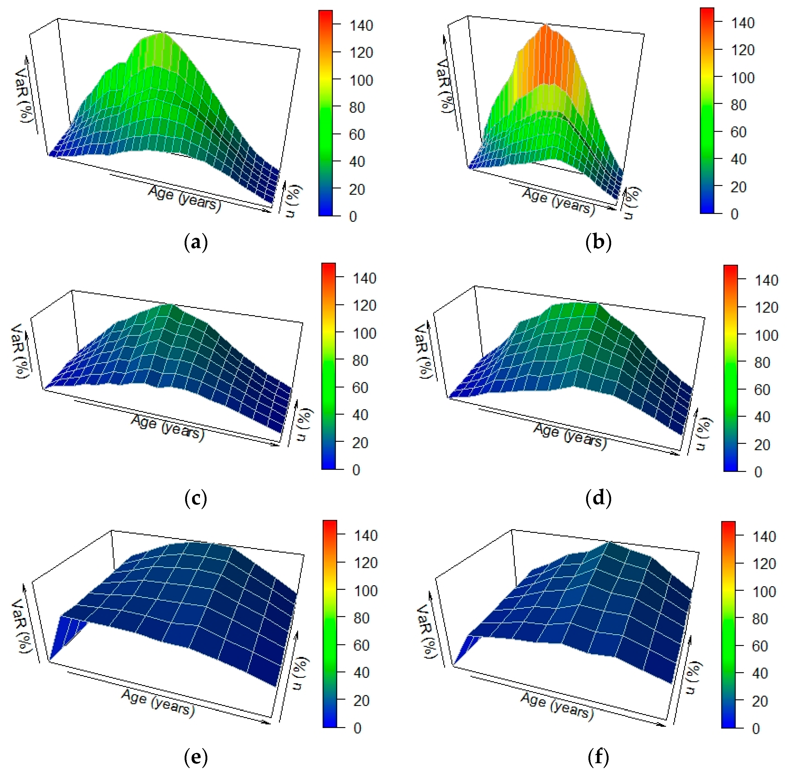
Figure 6.
One-year 99.9%VaR depending on the borrower’s age and on the mortgage roll-up rate as a percentage of the portfolio value at the beginning of each year. The figure shows the dependency of the one-year 99.9% VaR, expressed as a percentage of the value of the reverse mortgage portfolio at the beginning of each annual period, on the borrower’s age and the mortgage roll-up rate (u), for different borrower’s ages at inception and gender ((a) Male 70 y.o., (b) Female 70 y.o., (c) Male 80 y.o., (d) Female 80 y.o., (e) Male 90 y.o. and (f) Female 90 y.o.).

Figure 7.
One-year 99.9% VaR, as a percentage of the initial portfolio value at inception, depending on the borrower’s age and on the mortgage roll-up rate. The figure shows the dependency of the one-year 99.9% VaR, expressed as a percentage of the initial portfolio value at inception, on the borrower’s age and on the mortgage roll-up rate (u), for different borrower’s ages at inception and gender ((a) Male 70 y.o., (b) Female 70 y.o., (c) Male 80 y.o., (d) Female 80 y.o., (e) Male 90 y.o. and (f) Female 90 y.o.).

Figure 8.
Heat map for the one-year 99.9% VaR as a percentage of the initial portfolio value at the beginning of each annual period, depending on the borrower age and the mortgage roll-up rate. The heat map shows the dependency of the one-year 99.9% VaR, expressed as a percentage of the value of the reverse mortgage portfolio at the beginning of each annual period, on the borrower age and the mortgage roll-up rate (u), for different borrower ages at inception and genders ((a) Male 70 y.o., (b) Female 70 y.o., (c) Male 80 y.o., (d) Female 80 y.o., (e) Male 90 y.o. and (f) Female 90 y.o.).

Figure 9.
Heat map for the one-year 99.9% VaR as a percentage of the initial portfolio value at inception, depending on the borrower age and the mortgage roll-up rate. The heat map shows the dependency of the one-year 99.9% VaR, expressed as a percentage of the value of the reverse mortgage portfolio at inception, on the borrower age and the mortgage roll-up rate (u) and gender ((a) Male 70 y.o., (b) Female 70 y.o., (c) Male 80 y.o., (d) Female 80 y.o., (e) Male 90 y.o. and (f) Female 90 y.o.).


Table 1.
Summary of the main advantages and drawbacks of the existing papers on calculating the regulatory capital requirements for reverse mortgages compared to the present study.
Table 1.
Summary of the main advantages and drawbacks of the existing papers on calculating the regulatory capital requirements for reverse mortgages compared to the present study.
| Authors | Advantages | Drawbacks |
|---|---|---|
| Sun, D. & Sherris, M. [13] |
|
|
| Alai et al. [6] |
|
|
| Cho et al. [14] |
|
|
| The present study |
|
|
NNEG: no-negative-equity guarantee, GDP: gross domestic product, CPI: consumer price index, VaR: value at risk, ES: expected shortfall.
Table 2.
Descriptive Statistics. House price index (HPI) Log Return. The table shows the main descriptive statistics of the HPI log quarterly returns for the U.K. from 1952 Q4 to 2019 Q4.
Table 2.
Descriptive Statistics. House price index (HPI) Log Return. The table shows the main descriptive statistics of the HPI log quarterly returns for the U.K. from 1952 Q4 to 2019 Q4.
| HPI Log Return | |
|---|---|
| Mean | 0.02 |
| Median | 0.02 |
| Maximum | 0.12 |
| Minimum | −0.05 |
| Std. Dev. | 0.02 |
| Skewness | 0.64 |
| Kurtosis | 5.18 |
| Jarque-Bera | 70.92 |
| (Probability) | (0.00) |
| Observations | 268 |
Table 3.
Estimation Results. ARMA-EGARCH Model. The table shows the results of the estimation of the ARMA-EGARCH model for forecasting house price index returns for the U.K. from 1952 Q4 to 2019 Q4 (268 quarterly observations).
Table 3.
Estimation Results. ARMA-EGARCH Model. The table shows the results of the estimation of the ARMA-EGARCH model for forecasting house price index returns for the U.K. from 1952 Q4 to 2019 Q4 (268 quarterly observations).
| Parameter | Value | t-Stat. |
|---|---|---|
| c | 0.02 | 4.92 |
| φ1 | 0.81 | 16.53 |
| φ2 | −1.01 | −295.62 |
| φ3 | 0.80 | 16.32 |
| θ1 | −0.28 | −2.67 |
| Φ2 | 1.00 | 198.90 |
| θ3 | −0.26 | −2.51 |
| k | −1.29 | −3.18 |
| α1 | 0.42 | 4.95 |
| β1 | 0.89 | 19.58 |
| γ1 | 0.13 | 2.88 |
| AIC | −5.58 | |
| SBC | −5.43 | |
ARMA: autorregresive, moving-average, EGARCH: exponential generalized autorregresive conditional heteroskedasticity.
Publisher’s Note: MDPI stays neutral with regard to jurisdictional claims in published maps and institutional affiliations. |
© 2020 by the authors. Licensee MDPI, Basel, Switzerland. This article is an open access article distributed under the terms and conditions of the Creative Commons Attribution (CC BY) license (http://creativecommons.org/licenses/by/4.0/).
Share and Cite
MDPI and ACS Style
Fuente, I.d.l.; Navarro, E.; Serna, G. Reverse Mortgage Risks. Time Evolution of VaR in Lump-Sum Solutions. Mathematics 2020, 8, 2043. https://0-doi-org.brum.beds.ac.uk/10.3390/math8112043
AMA Style
Fuente Idl, Navarro E, Serna G. Reverse Mortgage Risks. Time Evolution of VaR in Lump-Sum Solutions. Mathematics. 2020; 8(11):2043. https://0-doi-org.brum.beds.ac.uk/10.3390/math8112043
Chicago/Turabian StyleFuente, Iván de la, Eliseo Navarro, and Gregorio Serna. 2020. "Reverse Mortgage Risks. Time Evolution of VaR in Lump-Sum Solutions" Mathematics 8, no. 11: 2043. https://0-doi-org.brum.beds.ac.uk/10.3390/math8112043
Note that from the first issue of 2016, this journal uses article numbers instead of page numbers. See further details here.