US Policy Uncertainty and Stock Market Nexus Revisited through Dynamic ARDL Simulation and Threshold Modelling

Abstract

Since the introduction of the measure of economic policy uncertainty, businesses, policymakers, and academic scholars closely monitor its momentum due to expected economic implications. The US is the world’s top-ranked equity market by size, and prior literature on policy uncertainty and stock prices for the US is conflicting. In this study, we reexamine the policy uncertainty and stock price nexus from the US perspective, using a novel dynamically simulated autoregressive distributed lag setting introduced in 2018, which appears superior to traditional models. The empirical findings document a negative response of stock prices to 10% positive/negative shock in policy uncertainty in the short-run, while in the long-run, an increase in policy uncertainty by 10% reduces the stock prices, which increases in response to a decrease with the same magnitude. Moreover, we empirically identified two significant thresholds: (1) policy score of 4.89 (original score 132.39), which negatively explain stock prices with high magnitude, and (2) policy score 4.48 (original score 87.98), which explains stock prices negatively with a relatively low magnitude, and interestingly, policy changes below the second threshold become irrelevant to explain stock prices in the United States. It is worth noting that all indices are not equally exposed to unfavorable policy changes. The overall findings are robust to the alternative measures of policy uncertainty and stock prices and offer useful policy input. The limitations of the study and future line of research are also highlighted. All in all, the policy uncertainty is an indicator that shall remain ever-important due to its nature and implication on the various sectors of the economy (the equity market in particular).

1. Introduction

The field of mathematical finance is one of the most rapidly emerging domains in the subject of finance. Dynamically Simulated Autoregressive Distributed Lag (DYS-ARDL) [1] is an influential tool that may help an investor analyze and benefit by understanding the positive and negative shocks in policy indicators. This strategy enables investors to observe the reaction of equity prices to positive and negative shocks of various magnitude (1%, 5%, 10%, and others). More importantly, it may assist the diversification of potential portfolios across various equities based on predicted reaction. Coupled with DYS-ARDL, the few other effective strategies include statistical arbitrage strategies (SAS) and pairs trading strategy (PTS) that are empirically executed in mathematical finance literature; see for example [1,2,3,4,5,6]. Stübinger and Endres [2] developed and applied PTS to minute-by-minute data of oil companies constituting the S&P 500 market index for the US and revealed that the statistical arbitrage strategy enables intraday and overnight trading. Similarly, Stübinger, Mangold, and Krauss [6] developed SAS (based on vine copulas), which is a highly flexible instrument with multivariate dependence modeling under the linear and nonlinear setting. The authors find it promising in the context of the S&P 500 index of the United States (US) equities. Using SAS, Avellaneda and Lee [3] related the performance of mean-reversion SAS with the stock market cycle and found it effective in studying stock performance during the liquidity crisis. Empirical evidence from the US equity market on PTS links trading cost documents that PTS is profitable among well-matched portfolios [5]. Liu, Chang, and Geman [4] argue that PTS can facilitate stakeholders to capture inefficiencies in the local equity market using daily data. Interestingly, we find that SAS and PTS strategies are successfully employed in the context of the US, while to the best of our knowledge, we do not find the use of DYS-ARDL, which is surprising. Each of the described strategies has unique features in a given scenario in which they are used, yet it worthwhile to add little value to mathematical finance literature by empirically examining the DYS-ARDL specification in the US context.

Given the economic implications of financial markets and eventual behavior [7,8,9,10], this piece of research empirically examines the short- and long-run impacts of policy uncertainty (hereafter PU) on stock prices of the US using a novel DYS-ARDL setting proposed by Jordan and Philips [1] and of threshold relation using the Tong [11] model. The study is motivated by conflicting literature on policy risk stock price and shortcomings associated with the traditional cointegration model (e.g., Autoregressive Distributed Lag (ARDL)).

Since the introduction of the measure of PU by Baker et al. [12], the effects of the PU on macro variables have gained substantial attention. PU is closely monitored and analyzed by businesses, policymakers, and academic scholars, as the global economy is now more closely interconnected than ever [13]. Intuitively, an increase in PU is expected to negatively influence the stock market, while on the contrary, stock market indicators may react positively to a decline in PU [14]. This intuition is consistent with the findings of Baker, Bloom, and Davis [12], who have shown its adverse effects on economic activities, which is confirmed by the recent literature [14,15,16,17,18,19,20,21,22,23,24,25,26,27].

According to Baker, Bloom, and Davis [12], economic PU refers to “a non-zero probability of changes in the existing economic policies that determine the rules of the game for economic agents”. The impact of changes in PU may potentially rout the following channels:

• First, it can change or delay important decisions made by companies and other economic actors, such as investment [28], employment, consumption, and savings decisions [14,29].
• Second, it increases financing and production costs by affecting supply and demand channels, exacerbating investment decline, and economic contraction [14,17,30,31].
• Third, it can increase the risks in financial markets, especially by reducing the value of government protection provided to the market [17].
• Lastly, PU also affects inflation, interest rates, and expected risk premiums [32,33].

Importantly, in the context of the US, the phenomena are also captured by a few studies [14,21,22,23,27] with conflicting findings. For example, some of them [14,15,21,23,34] found a negative relationship, while others reported no effect [22,27]. The conflicting referred literature on the US [14,15] relies on the classical approach [35] to capture the cointegration relationship. From the symmetry assumption perspective drawn on this approach [35], it follows that an increase in PU will negatively affect the other macroeconomic variables and that a decrease in PU will increase this variable. However, this may not be the case, as investors’ responses may differ from increasing PU versus decreasing PU. It is possible that, due to an increase in uncertainty, investors move their equity assets to safer assets and that a decrease in uncertainty may cause them to shift their portfolio towards the stock market (assume the change in PU is less than increase) if they expect that a decrease in uncertainty is short-lived and then that asymmetry originates.

The shortcomings associated with Pesaran, Shin, and Smith [35] are, to some extent, addressed by nonlinear extension by Shin et al. [36], which generates two separate series (positive and negative) from the core explanatory variable. Thus, the asymmetric impact may be estimated; however, this approach overlooks the simulation features while estimating the short- and long-run asymmetries. The package is given by Jordan and Philips [1], known as the DYS-ARDL approach, which takes into account the simulation mechanism and liberty to use positive and negative shocks in an explanatory variable and captures the impact in a variable of interest. According to recent literature [37,38], this novel approach is capable of predicting the actual positive and negative changes in the explanatory variable and its subsequent impact on the dependent variable. Moreover, it can stimulate, estimate, and automatically predict, and graph said changes. The authors also believe that classical ARDL can only estimate the long-term and short-term relationships of the variables. Contemplating the limitations associated with traditional estimators, this study uses Jordan and Philips [1] inspirational DYS-ARDL estimator to examine the relationship between PU and US stock prices.

In addition, this study extends the analysis beyond the DYS-ARDL estimator [1] by using Tong [11] threshold regression Although DYS-ARDL [1] is a powerful tool to capture the dynamic cointegration between an independent variable and dependent variable, and its unique feature automatically generates the simulation-based graph of changes to SP as a result of a certain positive/negative shock in PU, it is beyond its capacity to figure out a certain level (point) where the relationship (magnitude of coefficient) changes. For example, literature shows that the general stock market is linearity correlated with the changes in PU [14,15,16,17,18,19,20,21,22,23,24,25,26,27]. An increase in PU brings a negative influence on SP, in which a decrease translates into a positive change.

Threshold models have recently paid attention to modeling nonlinear behavior in applied economics. Part of the interest in these models is in observable models, followed by many economic variables, such as asymmetrical adjustments to the equilibrium [39]. By reviewing a variety of literature, Hansen [40] recorded the impact of the Tong [11] threshold model on the field of econometrics and economics and praised Howell Tong’s visionary innovation that greatly influenced the development of the field of econometrics and economics.

Concisely, this small piece of research extends the financial economics and mathematical finance literature on PU and SP in the context of the United States, which is the world’s top-ranked equity market [41] in three distinct ways. First, the novelty stems from the use of DYS-ARDL [1], which produces efficient estimation using simulations mechanism (which traditional ARDL departs), and auto-predicts the relationship graphically alongside empirical mechanics. To the best of our knowledge, this is the first study to verify traditional estimation with this novel and robust method. The empirical findings of DYS-ARDL document a negative response of stock prices in the short-run for a 10% positive and negative change (shock) in PU, while a linear relationship is observed in case of the long-run in response to said change.

Second, coupled with novel DYS-ARDL, this study adds value to relevant literature by providing evidence from threshold regression [11], which provides two significant thresholds in the nexus of PU-SP that may offer useful insight into policy matters based upon identified threshold(s). It is worth noting that SP negatively reacts to PU until a certain level (threshold-1), where the magnitude of such reaction changes (declines) to another point (threshold-2) with relatively low magnitude (still negative). Interestingly, below threshold-2, the PU became irrelevant to the US-SP nexus.

Third, this is a compressive effort to provide a broader picture of the US stock market reaction to policy changes. In this regard, prior literature is confined to the New York Stock Exchange Composite Index and S&P 500, while this study empirically tested seven major stock indices: S&P 500, Dow Jones Industrial Average, Dow Jones Composite Average, NASDAQ composite, NASDAQ100, and Dow Jones Transpiration Average. Expending analysis of these indices potentially provides useful insights to investors and policymakers because all are not equally exposed to adverse changes in PU. Some of them are nonresponsive to such changes, which may help a group of investors diversifying their investments to avoid unfavorable returns and to construct the desired portfolio with low risk. On the other hand, risk-seeking investors may capitalize on risk premiums, where understanding the identified thresholds may help to diversify their investments reasonably.

The rest of the work is organized as follows. Section 2 outlines the related literature; Section 3 illustrates the material and methods; results and discussion are covered by Section 4; the study is concluded in Section 5.

2. Literature Review

Bahmani-Oskooee and Saha [15] assessed the impact of PU on stock prices in 13 countries, including the United States, and find that, in almost all 13 countries, increased uncertainty has negative short-term effects on stock prices but not in the long term. Sum [18] utilized the ordinary least squares method to analyze the impact of PU on stock markets (from January 1993 to April 2010) of Ukraine, Switzerland, Turkey, Norway, Russia, Croatia, and the European Union. The study finds that PU negatively impacts EU stock market returns, except for in Slovenia, Slovakia, Latvia, Malta, Lithuania, Estonia, and Bulgaria. The analysis does not identify any negative impact of stock market returns of non-EU countries included in the study. Sum [24] used a vector autoregressive model with Granger-causality testing and impulse response function and founds that PU negatively impacts stock market returns for most months from 1985 to 2011.

Another study [34] analyzed monthly data of PU and stock market indices of eleven economies, including China, Russia, the UK, Spain, France, India, Germany, the US, Canada, Japan, and Italy. The study found that PU negatively impacts stock prices mostly except periods of low-to-high frequency cycles. The study used data from 1998 to 2014. Using data from 1900 to 2014, Arouri, Estay, Rault, and Roubaud [14] measured PU’s impact on the US stock market and found a weak but persistent negative impact of PU on stock market returns. Inflation, default spread, and variation in industrial production were the control variables used. The study also found that PU has a greater negative impact on stock market returns during high volatility.

Pastor and Veronesi [17] estimated how the government’s economic policy announcement impacts stock market prices and reported that stock prices go up when the government makes policy announcements and that more unexpected announcement brings in greater volatility. Li, Balcilar, Gupta, and Chang [19] found a weak relationship between PU and stock market returns in China and India. For China, the study used monthly data from 1995 to 2013, and for India, it used monthly data from 2003 to 2013. The study employed two methods (i) bootstrap Granger full-sample causality testing and (ii) subsample rolling window estimation. The first method did not find any relationship between stock market returns and PU, while the second method showed a weak bidirectional relationship for many sub-periods. Employing the time-varying parameter factor-augmented vector autoregressive (VAR) model on data from January 1996 to December 2015, Gao, Zhu, O’Sullivan, and Sherman [20] estimated the impact of PU on the UK stock market returns. The study considered both domestic and international economic PU factors. The paper maintains that PU explains the cross-section of UK stock market returns.

Wu, Liu, and Hsueh [22] analyzed the relationship between PU and performance of the stock markets of Canada, Spain, the UK, France, Italy, China, India, the US, and Germany. Analyzing monthly data from January 2013 to December 2014, the study found that not all stock markets under investigation react similarly to PU. According to the study, the UK stock market falls most with negative PU, but the markets of Canada, the US, France, China, and Germany remain unaffected. Asgharian, Christiansen, and Hou [21] measured the relationship between PU and the US (S&P 500) and the UK (FTSE 100) stock markets. The study used daily data for stock market indices and monthly data for PU. The paper found that stock market volatility in the US depends on PU in the US and that stock market volatility in the UK depends on PU in both the US and UK.

Christou, Cunado, Gupta, and Hassapis [23] estimated the impact of PU on the stock markets of the US, China, Korea, Canada, Australia, and Japan. Using monthly data from 1998 to 2014 and employing a panel VAR model with impulse response function, the study found that own country PU impacts stock markets negatively in all aforementioned countries. The study also found that PU in the US also negatively impacts all other countries’ stock markets in the analysis, except Australia. Debata and Mahakud [25] found a significant relationship between PU and stock market liquidity in India. The study used monthly data from January 2013 to Granger 2016 and employed VAR Granger causality testing, variance decomposition analysis, and impulse response function. The impulse response function showed that PU and stock market liquidity are negatively related.

Liu and Zhang [42] investigated PU’s impact on stock market volatility of the S&P 500 index from January 1996 to June 2013. The study found that PU and stock market volatility are interconnected and that PU has significant predictive power on stock market volatility. Pirgaip [27] focused on the relationship between stock market volatility for fourteen OECD countries, subject to monthly data from March 2003 to April 2016 for Japan, France, Germany, Chile, Canada, Italy, Australia, the US, UK, Sweden, Spain, Netherlands, Australia, and South Korea. Employing the bootstrap panel Granger causality method, the study found that PU impacts stock prices in all countries except the US, Germany, and Japan.

Škrinjarić and Orlović [26] estimated the spillover effects of PU shocks on stock market returns and risk for nine Eastern and Central European countries, including Bulgaria, Estonia, Lithuania, Croatia, Slovenia, Hungary, Czech Republic, Poland, and Slovakia. The paper employed a rolling estimation of the VAR model and the spillover indices. The study’s findings suggest that Poland, the Czech Republic, Slovenia, and Lithuania are more sensitive to PU shocks compared to other markets in the study. In contrast, the Bulgarian stock market is least impacted by PU shocks. Other countries’ stock markets have an individual reaction to PU shocks.

Ehrmann and Fratzscher [43] examined how the US monetary policy shocks are transmitted stock market returns over February 1994 to December 2004, with a weak association in India, China, and Malaysia’s stock markets while strong on Korea, Hong Kong, Turkey, Indonesia, Canada, Finland, Sweden, and Australia. Brogaard and Detzel [44] examined the relationship between PU and asset prices using a monthly Center for Research in Security Prices (CRSP) value-weighted index as the US stock market’s performance measure and PU. The findings suggest that a one standard deviation increase in PU decreases stock returns by 1.31% and increases 3-month log excess returns by 1.53%. The study also found that dividend growth is not affected by PU. Antonakakis et al. [45] estimated co-movements between PU and the US stock market returns and stock market volatility using S&P 500 stock returns data and S&P 500 volatility index data. The study found a negative dynamic correlation between PU and stock returns except during the financial crisis of 2008, for which the correlation became positive.

Stock market volatility also negatively impacts the stock market returns, according to the study. Dakhlaoui and Aloui [46] scrutinized the relationship between the US PU and Brazil, Russia, India, and China stock markets, estimating daily data from July 1997 to July 2011. The study found a negative relationship between the US PU and the returns, but the volatility spillovers were found to oscillate between negative and positive making, it highly risky for investors to invest in US and BRIC stock markets simultaneously. Yang and Jiang [47] used data from the Shanghai stock index from January 1995 to December 2014 to investigate the relationship between PU and china stock market returns and suggest that stock market returns and PU are negatively correlated and that the negative impact of PU lasts for about eight months after the policy announcement.

Das and Kumar [16] estimated the impacts of domestic PU and the US PU on the economies of 17 countries. The analysis included monthly data from January 1998 to February 2017 and found that emerging markets are less prone and vulnerable to domestic and US PU than developed economies while Chile and Korea are relatively more sensitive to both Domestic PU and US PU, whereas China is least affected. Estimation reveals that except Canada and Australia, stock prices and all other developed economies in the analysis are quite sensitive to US PU. Australia and Canada stock prices are more reliant on domestic PU. Stock prices of all the emerging economies are more reliant on domestic PU except for the marginal exception of Russia and Brazil.

We conclude that the reviewed literature on policy-stock prices is conflicting. See, for example, Bahmani-Oskooee and Saha [15]; Asgharian, Christiansen, and Hou [21]; Christou, Cunado, Gupta, and Hassapis [23]; Ko and Lee [34]; and Arouri, Estay, Rault, and Roubaud [14], who found that the US stock market is negatively correlated to changes in PU, and Wu, Liu, and Hsueh [22], and Pirgaip [27], who documented no effect of US. Sum [13] revealed a cointegration relationship that exists between the economic uncertainty of the US and Europe, showing a spillover effect across financial markets across the national borders. The literature referred to the US with few exceptions including Arouri, Estay, Rault, and Roubaud [14], and Bahmani-Oskooee and Saha [15], who assumed a linear relationship between PU and stock prices and relied on Pesaran, Shin, and Smith [35] for the traditional cointegration approach to finding the long-run dynamics of the PU and stock prices. Amongst these, Arouri, Estay, Rault, and Roubaud [14] found a long-run weak negative impact in general and persistent negative impact during high volatility regimes. However, Bahmani-Oskooee and Saha [15] found short-run negative impacts and no effect in the long-run.

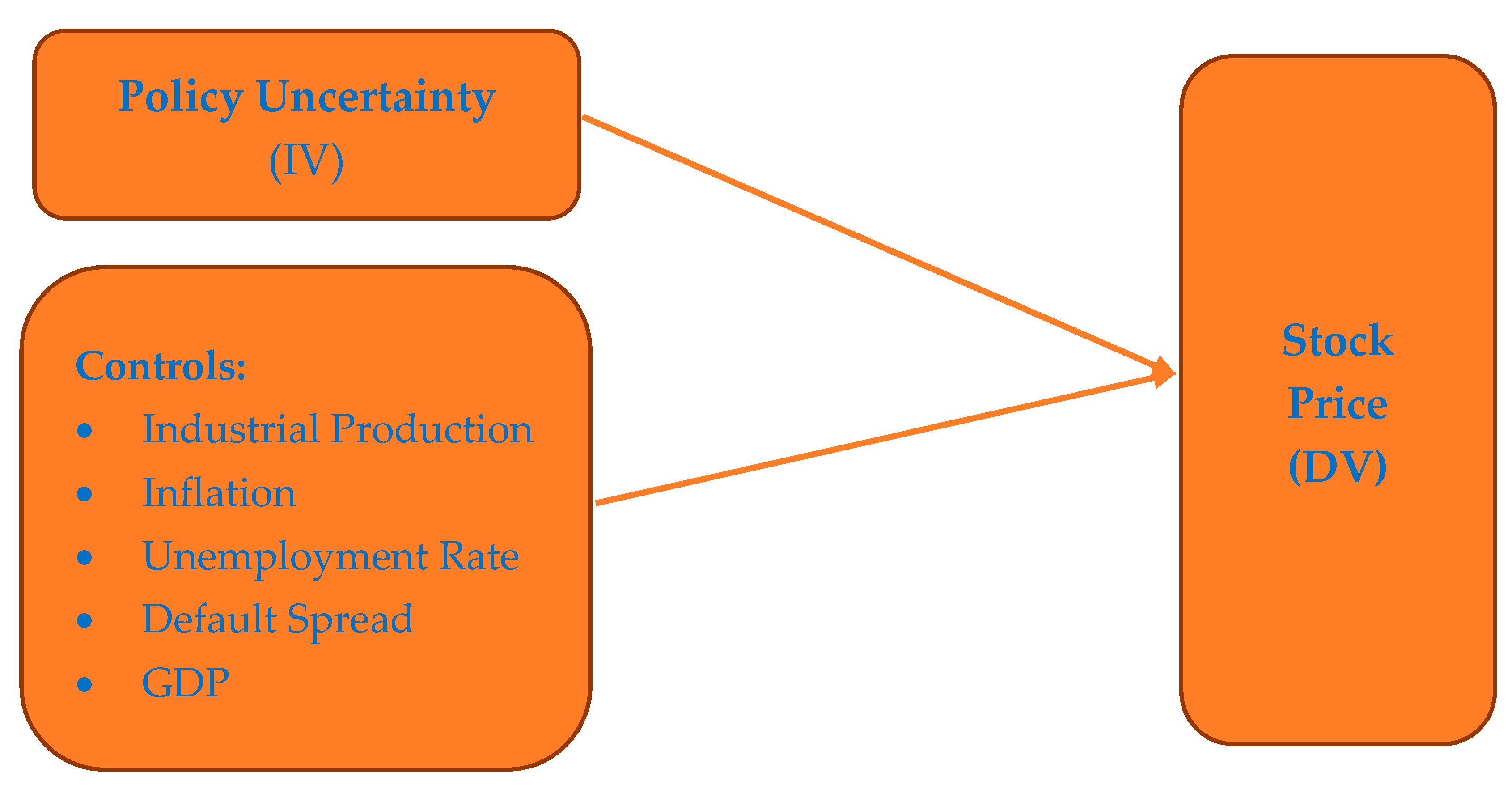
The strand of literature relied on traditional cointegration [35] for modeling policy-stock price connection follows the symmetry assumption perspective holding that an increase in PU will negatively affect the other macroeconomic variable and a decrease in PU will increase this variable. However, this may not be the case, as investors’ responses may differ from increasing PU versus decreasing PU. It is possible that, due to an increase in uncertainty, investors move their equity assets to safer assets and that a decrease in uncertainty may cause them to shift their portfolio towards the stock market (assume the change in PU is less than increase) if they expect that a decrease in uncertainty is short-lived and then that asymmetry originates. Figure 1 plots the theoretical framework based on reviewed papers [14,15].

We conclude that empirical literature on PU and stock prices is conflicting, with no consensus on its empirical impact, as the literature shows mixed results (positive, negative, and no effect). This may be attributable to the differences in methodological strategies used, time coverage, and other controls used in the estimation process. Among empirical methods used, ARDL is commonly used to arrive at short- and long-run cointegration relationships. Moreover, it is surprising that threshold identification in PU and stock price connection is an unaddressed phenomenon. Thus, it is imperative to go ahead and comprehensively examine the short- and the long-run association between PU and stock prices using an updated dataset coupled with DYS-ARDL and the threshold strategy in the context of the United States, the world top-ranked financial market (in terms of market size) [41].

3. Materials and Methods

3.1. Description of Variables and Data Source

The independent variable is economic PU, which is an index built by Baker, Bloom, and Davis [12] from three types of underlying components. The first component quantifies the news coverage of policy-related economic uncertainties. A second component reflects the number of federal tax legislation provisions that will expire in the coming years. The third component uses the disagreement among economic meteorologists as an indicator of uncertainty. The first component is an index of the search results of 10 major newspapers, which includes US Today, Miami Herald, Chicago Tribune, Washington Post, Los Angeles Times, Boston Globe, San Francisco Chronicle, Dallas Morning News, New York Times, and Wall Street Diary. From these documents, Baker, Bloom, and Davis [12] create a normalized index of the volume of news articles discussing PU. The second component of this index is based on reports from the congressional budget office, which compiles lists of temporary provisions of federal tax legislation. We compile an annual number of weighted US dollar tax laws that expire over the next 10 years and provide a measure of uncertainty on which path federal tax laws will follow in the future.

The third component of the PU index is based on the Federal Reserve Bank of Philadelphia’s survey of professional meteorologists. Here, it uses the dispersion between individual meteorologists’ forecasts of future consumer price index levels, federal spending, and state and local spending to create indices of uncertainty for policy-related macroeconomic variables. This study uses news-based PU (PU_NB) for the main analysis, while robustness is performed using three component-based PU index (PU_3C). Figure 2 provides a glimpse of historical US monthly PU indices (both PU_NB and PU_3C). A rise in PU indices is shown by the second half of the sample period. We may attribute it to a series of incidents, such as the 9/11 attack on the World Trade Centre, followed by US coalition attack on Afghanistan in 2001, mounted tension between the US and North Korea in 2003, and the US attack on Iraq in 2003. Later, the major event was the 2007–2009 recession in the form of a US economic crash caused by the subprime crisis in 2008, and aftershocks in subsequent years have significantly raised the PU. The efforts to reduce carbon emission have caused an economic downturn in 2010–2011, US economic slowdown was heavily weighted by the global economic slowdown in 2015–2016, and finally, the sizable swaths of US economic shutdown were a result of COVID-19.

This study utilizes monthly data ranging from January 1985 to August 2020. For this period, data on PU is downloaded from the economic PU website (http://www.policyuncertainty.com/), which is open-source and commonly used in related literature, while data on seven US stock market indices are accessed from Yahoo Finance [48]. This includes monthly adjusted closing stock prices of the New York Stock exchange composite index (NYSEC) as a dependent variable for baseline analysis; however, the same measure of S&P500, Dow Jones Industrial Average (DJI), Dow Jones Composite Average (DJA), NASDAQ composite, NASDAQ100, and Dow Jones Transpiration Average (DJT) are utilized as robustness. Following Arouri, Estay, Rault, and Roubaud [14], and Bahmani-Oskooee and Saha [15], we consider Industrial production (IP), default spread (DS), inflation (INF), and unemployment rate (UE) as potential controls, and monthly data are sourced from Federal Reserve Economic Data (FRED https://fred.stlouisfed.org/) [49]. FRED is an open-source database that maintains various frequency datasets on more than 0.07 million in the United States and international time-series data from above 100 date sources.

The choice of the US’s stock market as a potential unit for analysis is led by its top rank in terms of size among world exchanges [41]. Figure 3 shows a list of the world’s largest stock exchanges as per the market capitalization of listed companies. The New York stock exchange and NASDAQ are ranked first and second with 25.53 and 11.23 trillion US dollars, respectively, among world exchanges [41].

Table 1. Descriptive Statistics.

Abbreviation	Description	Measurement	Mean	Std.Dev.	Min	Max	Data Source
SP	Stock price	Natural log of adjusted closing prices of NYSE composite index	8.538	0.702	7.000	9.541	Yahoo Finance https://finance.yahoo.com/
PU_NB	News-based policy uncertainty	Natural log of news-based policy uncertainty index	4.692	0.378	3.802	6.223	http://www.policyuncertainty.com/
INF	Inflation	Natural log	5.181	0.260	4.659	5.560	FRED https://fred.stlouisfed.org/
IP	Industrial production	Natural log	4.439	0.248	1.716	4.705
UE	Unemployment rate	%	5.947	1.647	3.500	14.700
DS	Default spread	Moody’s Seasoned Baa Corporate Bond Minus Federal Funds Rate	3.847	1.596	0.500	8.820

shows the descriptive properties of the underlying variables.

Jordan and Philips’s [1] DYS-ARDL can be expressed in the following standard pathway:

$$\begin{array}{c}∆{\left(y\right)}_t={\alpha }_0+{\theta }_0{\left(y\right)}_{t-1}+{\theta }_1{\left(x_1\right)}_{t-1}+\dots +{\theta }_k{\left(x_k\right)}_{t-1}+{\displaystyle {\displaystyle \sum }_{i=1}^p}{\alpha }_{0i}∆{\left(y\right)}_{t-1}+{\displaystyle {\displaystyle \sum }_{j=0}^{q1}}{\beta }_{1j}∆{\left(x_1\right)}_{t-j}+\dots \\ +{\displaystyle {\displaystyle \sum }_{j=0}^{qk}}{\beta }_{kj}∆{\left(x_k\right)}_{t-j}+{\epsilon }_t\end{array}$$

(1)

where the change in the dependent variable (y) is a function of the intercept (${\alpha }_0$), and all the independent variables at time $t-1$ are the levels of the maximum of $p$ and $qk$ lags in respective first difference $(∆)$ along with error term $\left(\epsilon \right)$ at time $t$. The study uses Pesaran, Shin, and Smith’s [35] ARDL bounds testing approach for a level relationship using Kwiatkowski–Phillips–Schmidt–Shin (2018) critical values as a benchmark. The null hypothesis for no level relationship obtained by joint F-statistics from the estimation is rejected against the critical bounds, in particular, when estimated F-statistics is greater than the upper bound I(1). Drawn on the empirical specification illustrated in Equation (1), the error correction transformation of the ARDL bounds estimators are estimated under the following:

The change in the dependent variable (y) is a function of intercept (${\alpha }_0$), and all the independent variables at time $t-1$ are levels to the maximum of $p$ and $qk$ lags in respective first difference $(∆)$ along with error term $\left(\epsilon \right)$ at time $t$. The study uses Pesaran, Shin, and Smith’s [35] ARDL bounds testing approach for a level relationship using Kwiatkowski–Phillips–Schmidt–Shin (2018) critical values as a benchmark. The null hypothesis for no level relationship obtained by joint F-statistics from the estimation is rejected against the critical bounds, in particular, when estimated F-statistics is greater than the upper bound I(1). Drawn on the empirical specification illustrated in Equation (1), the error correction transformation of the ARDL bounds estimators are estimated as under the following:

$$\begin{array}{cc}∆ln{\left(SP\right)}_t={\alpha }_0& +{\theta }_0 ln {\left(SP\right)}_{t-1}+{\beta }_1∆ ln {\left(PU\_NB\right)}_t+{\theta }_1 ln {\left(PU\_NB\right)}_{t-1}+{\beta }_2∆ ln {\left(INF\right)}_t\\ & +{\theta }_2 ln {\left(INF\right)}_{t-1}+{\beta }_3∆ ln {\left(IP\right)}_t+{\theta }_3 ln {\left(IP\right)}_{t-1}+{\beta }_4∆ {\left(UE\right)}_t+{\theta }_4{\left(UE\right)}_{t-1}\\ & +{\beta }_5∆ {\left(DS\right)}_t+{\theta }_5{\left(DS\right)}_{t-1}+{\epsilon }_t\end{array}$$

(2)

In Equation (2), ${\theta }_0$ denotes error correction term (ECT), ${\beta }_1-{\beta }_5$ capture the short-tun coefficient, and ${\theta }_1-{\theta }_5$ indicate a long-run coefficient for each of the regressors respectively.

3.2. Threshold Regression

The DYS-ARDL [1] is a powerful tool for capturing the dynamic cointegration between the independent variable and the dependent variable. Its unique function is to simulate the automatic generation of graphs based on changes in the dependent variable as a result of a certain positive/negative shock in the explanatory variable. However, any particular degree (point) of change in the relationship cannot be imagined. For example, the literature shows that linearity on the general stock market is related to changes in PU. The increase in PU harms the stock market, while the decrease in PU leads to positive changes.

The threshold model extends linear regression to allow the coefficients to vary among regions/regimes. These regions are identified by threshold variables that are greater or less than the threshold value. The model can have multiple thresholds; you can specify a known number of thresholds, or you can allow it to use Bayesian Information Criteria (BIC), Akaike Information Criteria (AIC), or Hannan–Quinn Information Criteria (HQIC to determine the number for you). It includes region-varying coefficients for specified covariates for each identified threshold, and it is efficient in automatically estimating the possible thresholds using the n thresholds(#) function. Moreover, it creates a variable with a sum of squared residuals for each tentative threshold. Thus, single threshold regression [11] is modeled by Equation (3).

The threshold model provides a systematic method of tracking the turning point in the relationship that can help decision-makers make better decisions [50,51,52,53]. Therefore, the threshold regression model for a single threshold [11] is modeled by Equation (3) for regions defined by threshold $\gamma$.

$$\begin{array}{l}{y}_t=X_t\beta +Z_t{\delta }_1+{\epsilon }_t if w_t \le \gamma \\ y_t=X_t\beta +Z_t{\delta }_2+{\epsilon }_t if \gamma < w_t\end{array}$$

(3)

where $y_t$ is a dependent variable (SP in our case), $X_t$ represents the vector consisting of region-invariant parameters (INF, IP, UE, and DS), $Z_t$ is a vector of exogenous variables with region-specific coefficient vectors (${\delta }_1 and {\delta }_2)$, and $w_t$ is the threshold variable, PU_NB (that may be one of the variables in $X_t$ or $Z_t$.

4. Results

4.1. Unit-Root Analysis

The preliminary step to test the level relationship between the dependent variable (SP) and respective regressors is to satisfy the stationarity condition of the individual series; in particular, the dependent variables must be integrated at the first difference, I(1). Furthermore, all the independent variables must not be stationary at the second difference, I(2). To determine the integration order aligned with recent literature [37], this study uses the Augmented Dickey–Fuller (ADF) and Kwiatkowski–Phillips–Schmidt–Shin (KPSS) test [54]. The null hypothesis for ADF assumes unit-root, while Baum [55] STATA module for KPSS, on the other hand, is tested under the null hypothesis of stationarity. The results are reported in

Table 2. Unit-root analysis.

Variable	Augmented Dickey–Fuller Test		Kwiatkowski–Phillips–Schmidt–Shin Test
	Level	1st Difference	Level	1st Difference
SP	−2.450	−10.413 ***	0.425	0.037 ***
PU_NB	−2.676	−4.950 ***	0.336	0.011 ***
INF	−1.270	−10.619 ***	0.879	0.030 ***
IP	−3.513 **	−4.637 ***	0.141 **	0.097 ***
UE	−2.798	−12.726 ***	0.499	0.041 ***
DS	−3.477 ***	−8.201 ***	0.134 **	0.063 ***

***, and ** indicate that the null hypothesis of unit-root rejected at 1%, 5%, and 10% levels of significance, respectively.

, which reveals that the null hypothesis for most of the underlying variables cannot be rejected at level, which is rejected at first difference. Both tests (ADF and KPSS) witness that the dependent variable is stationary at the first difference and that none of the regressors is integrated at second order. The situation calls for the potential use of ARDL bounds testing for cointegration. After determining the stationarity conditions, the selection of optimal lag is another essential and challenging task, for which there is no hard and fast rule. However, following Bahmani-Oskooee and Saha [15], and Bahmani-Oskooee and Saha [56], we allow 8–12 lags for monthly data in this study. The lag-order is determined using AIC, SC, and HQ.

4.2. Baseline Analysis—ARDL Bounds Test

The study estimates the baseline relationship between PU_NB and SP using ordinary least squared regression (OLS) in a series of estimation. Referring to

Table A1. OLS baseline results.

	(1)	(2)	(3)	(4)	(5)
	SP	SP	SP	SP	SP
PU_NB	0.443 ***	−0.220 ***	−0.186 ***	−0.124 ***	−0.105 ***
	(0.072)	(0.021)	(0.029)	(0.022)	(0.022)
INF		0.717 ***	0.481 ***	0.531 ***	0.556 ***
		(0.023)	(0.228)	(0.186)	(0.150)
IP			0.301	0.269	0.176
			(0.280)	(0.226)	(0.189)
DS				−0.053 ***	−0.029 ***
				(0.005)	(0.007)
UE					−0.040 ***
					(0.009)
Constant	0.460 ***	−0.505 ***	−0.776 ***	−0.986 ***	−0.646 ***
	(0.343)	(0.130)	(0.205)	(0.165)	(0.208)
Obs.	428	428	428	428	428
R-squared	0.057	0.944	0.948	0.961	0.965

Standard errors are in parenthesis. *** p < 0.01. All the abbreviations are defined in Table 1.

(Appendix A), initially in the model (1), PU_NB shows a positive impact on SP; however, when controls are introduced, the relationship becomes negative and consistent across all estimators (2–5). This shows the relevance of controls, and the inclusion of each control has increased the R-squared.

Pesaran, Shin, and Smith;s [35] bounds test reveals the existence of a cointegration relationship between PU_NB and SP along with controls.

Table 3. ARDL bounds test and diagnostic testing.

Test Statistics	Value
F-statistics	6.574
t-statistics	−4.654
Confidence interval	10%		5%			1%
Bounds	I(0)		I(1)	I(0)	I(1)	I(0)	I(1)
F-stat *	2.130		3.240	2.459	3.640	3.155	4.470
t-stat *	−2.557		−4.065	−2.857	−4.399	−3.439	−5.023
Diagnostic testing
Diagnostic test	Jarque-Bera		ARCH		Breusch-Pagan/Cook-Weisberg	Breusch-Godfrey LM	Ramsey RESET
p-value	0.188		0.101		0.102	0.418	0.452
Inference	Estimated residuals are normal		No heteroskedasticity problem			No serial correlation problem	Model correctly specified
Variance inflation factor
Variable	INF	IP	UE		DS	PU_NB	Mean VIF
VIF	2.94	2.8	2.18		1.85	1.43	2.15

* indicates Kripfganz and Schneider (2018) critical values.

shows the ARDL bounds test and diagnostic testing for baseline estimation. Computed absolute F-statistics and t-statistics in Table 3 (upper part) are greater than upper bounds at all significance levels (10%, 5%, and 1%) of Kripfganz and Schneider (2018) critical values.

After establishing the ARDL bounds test, we proceed to check for diagnostic testing. Table 3 (middle part) shows the p-values for each of the estimated tests, which affirms that baseline, and ARDL estimation satisfies the diagnostic properties, such as normality of estimated residuals, heteroskedasticity, serial correlation, and correct specification of the model. The bottom part of Table 3 incorporates the multicollinearity results of the variance inflation factor (VIF). The benchmark to draw inference is the individual VIF value for each regressor not being greater than 5. In our case, none of the regressors violate these criteria, which signifies that the multicollinearity problem does not exist in our estimation and that the obtained results are correctly estimated.

4.3. Dynamic ARDL Simulations and Robustness

Table 4. Dynamically simulated autoregressive distributed lag (DYS-ARDL) results.

	(1)	(2)
Variables	SP	SP
	PU_NB	Robustness: PU_3C
ECT(−1)	−0.067 ***	−0.072 ***
	(0.021)	(0.021)
∆PU	−0.044 ***	−0.068 ***
	(0.008)	(0.012)
PU	−0.014 **	−0.024 **
	(0.007)	(0.010)
∆INF	−0.096	−0.224
	(0.651)	(0.649)
INF	0.088 **	0.092 **
	(0.035)	(0.043)
∆IP	−0.008	−0.010
	(0.015)	(0.015)
IP	0.128 **	0.129 **
	(0.056)	(0.055)
∆UE	0.008 **	0.008 **
	(0.004)	(0.004)
UE	0.005 **	0.006 ***
	(0.002)	(0.002)
∆DS	−0.030 ***	−0.029 ***
	(0.007)	(0.007)
DS	−0.007 ***	−0.007 ***
	(0.002)	(0.002)
Constant	−0.368 ***	−0.360 ***
	(0.134)	(0.134)
Obs.	427	427
F-statistics	10.95 ***	10.21 ***
Simulations	5000	5000

Standard errors are in parenthesis. *** p < 0.01, and ** p < 0.05. All the abbreviations are defined in Table 1. SP refers to the NYSE composite index.

documents the results of DYS-ARDL [1], using PU_NB as a baseline measure (Table 4, model-1) and PU_3C as its near alternative for robustness (Table 4, model-2); 5000 simulations are estimated for both models. Khan, Teng, and Khan [37], and Khan et al. [57] affirm that the novel DYS-ARDL model can stimulate, estimate, and graph to automatically predict the graphs of negative and positive changes occurring in variables and their short- and long-term relationships, which are beyond the capacity of classical ARDL. The significant and negative coefficient of error correction term (ECT) in each of the estimated model stratifies the existence of a cointegration relationship between variables under consideration. The system corrects the previous period disequilibrium at a monthly rate of 6.7%. The negative and significant PU_NB coefficient illustrates that equity markets in the US do not like a mounting risk in the form of PU.

This study performed several robustness checks using an alternative measure of PU_NB and SP. A three component-based measure of PU is used as an alternative measure (it is explained in detail in the variable description section of the Material and Methods section). Table 4 (model-2) incorporates the results of DYS-ARDL, where the dependent variable is SP from the NYSEC index and the independent variable is PU_3C. The results are consistent with the main analysis. The disequilibrium is corrected at a monthly speed of adjustment of 7%, while both in the short- and long-run, increasing PU negatively drives the SP. Similar to the main analysis, the behavior of defaults spread is aligned to the implication of PU both in the short- and long-run. We find inflation, industrial production, and unemployment as stock-friendly indicators in the long-run with positive stimulus.

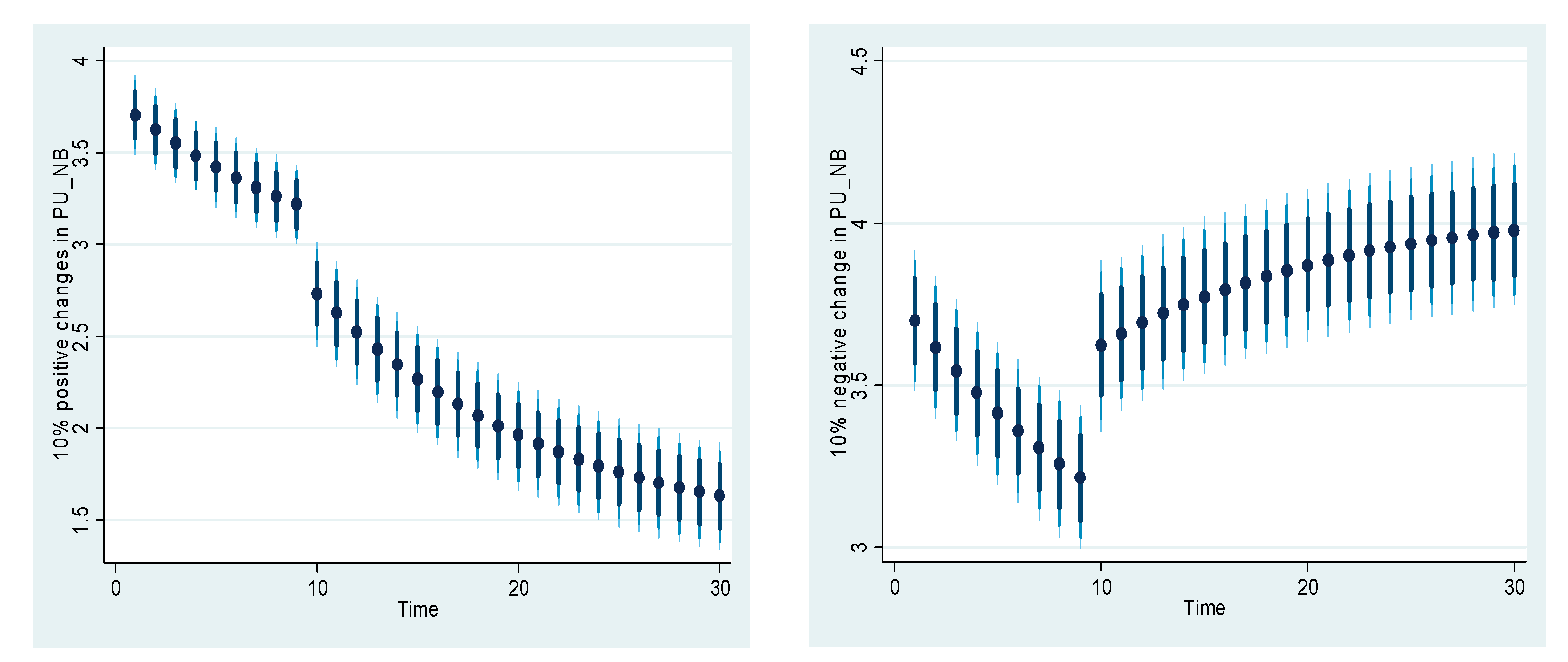
The impulse response function of the PU_NB impact on SP in the United States for the sampling period is shown in Figure 4. The results of the impulse response graph show that a 10% increase in PU_NB negatively affects the SP in the US both in the short- and long term while a 10% drop in the PU_NB shows negative effects in the US in the short term and positive effects in the long term. A short-term decline in SP because of PU_NB may be attributable to standard investment behavior, which is depicted by declining risk premium, which constitutes a substantial part of security prices. However, in the long run, the disequilibrium is corrected as shown by ECT in Table 4, and investment patterns are adjusted according to the risk.

4.4. Robustness: Alternative Measures of Stock Prices

Apart from the main analysis, the study explores the matter in depth by using six alternative stock indices (S&P 500, Dow Jones Industrial Average, Dow Jones Composite Average, NASDAQ Composite, NASDAQ 100, and Dow Jones Transpiration Average) from the United States for robustness.

Table A2. Robustness: alternative measures of SP.

	(1)	(2)	(3)	(4)	(5)	(6)
	SP_DJI	SP_DJA	SP_SP	SP_NASDAQC	SP_NASDAQ100	SP_DJT
ECT(−1)	−0.027 *	−0.048 ***	−0.016	−0.012	−0.011	−0.075 ***
	(0.016)	(0.018)	(0.014)	(0.012)	(0.011)	(0.023)
∆PU_NB	−0.045 ***	−0.041 ***	−0.042 ***	−0.066 ***	−0.068 ***	−0.054 ***
	(0.008)	(0.008)	(0.008)	(0.012)	(0.014)	(0.012)
PU_NB	−0.006 ***	−0.007 **	0.004	0.006	0.006	−0.008 ***
	(0.002)	(0.003)	(0.007)	(0.010)	(0.012)	(0.003)
Constant	−0.162	−0.338 **	−0.127	−0.167	−0.195	−0.510 ***
	(0.127)	(0.137)	(0.125)	(0.154)	(0.212)	(0.187)
Obs.	427	427	427	427	418	343
F-statistics	5.92 ***	6.11 ***	5.95 ***	5.48 ***	4.51***	4.52 ***
Simulations	5000	5000	5000	5000	5000	5000

Standard errors are in parenthesis. *** p < 0.01, ** p < 0.05, and * p < 0.1. DJI: Dow Jones Industrial Average, DJA: Dow Jones Composite Average, S&P: S&P 500, NASDAQ Composite, NASDAQ100, and DJT: Dow Jones Transpiration Average. Controls are not shown in this table as they are the same as estimated in the baseline model.

(Appendix B) uncovers interesting scenarios across the alternative measure so stock prices. Out of six alternatives, DJI, DJA, and DJT show a cointegration relationship to changes in PU, while other measures show negative but insignificant coefficients. One important phenomenon is the persistent negative reaction of all these measures to policy change in the short-run, while in the long-run, the response is negligible, and in particular, S&P 500, NASDAQ composite, and NASDAQ 100 are even not exposed to such a risk. These findings are encouraging for potential investors to diversify the investment across potential portfolios considering these reactions.

4.5. Threshold Regression

Table 5. Threshold regression results.

	PU_NB		Robustness: PU_3C
	(1)	(2)	(3)	(4)
Variables	SP	SP_S&P 500	SP	SP_S&P 500
TH-1	4.89 **		4.89 **
TH-2	4.48 **		4.48 **
INF	0.873 ***	1.017 ***	0.877 ***	0.987 ***
	(0.123)	(0.184)	(0.125)	(0.187)
IP	2.291 ***	2.080 ***	2.278 ***	2.098 ***
	(0.150)	(0.223)	(0.152)	(0.228)
GDP	−4.167 ***	−7.293 ***	−3.921 ***	−6.560 ***
	(0.983)	(1.467)	(0.914)	(1.366)
DS	−0.016 ***	0.008	−0.015 **	−0.043 ***
	(0.006)	(0.009)	(0.006)	(0.010)
UE	−0.023 *	−0.104 ***	−0.020 *	−0.048 ***
	(0.012)	(0.017)	(0.011)	(0.009)
PU ≥ Th-1	−0.291 ***	−0.270 ***	−0.174 **	−0.092 ***
	(0.077)	(0.093)	(0.093)	(0.016)
PU ≥ Th-2& ≤ TH-1	−0.074 **	−0.005 ***	−0.071 ***	−0.038 ***
	(0.034)	(0.002)	(0.011)	(0.014)
PU < TH-2	0.031	0.104	0.026	0.067
	(0.046)	(0.069)	(0.077)	(0.055)
Constant	13.086 ***	25.987 ***	12.111 ***	22.783 ***
	(4.459)	(6.657)	(4.219)	(6.304)
Obs.	428	428	428	428

Standard errors are in parenthesis. *** p< 0.01, ** p < 0.05, and * p < 0.1. The economic meanings of thresholds 4.89 and 4.48 are equivalent to the original PU_NB scores of 132.39, and 87.98, respectively. SP refers to the NYSE composite index.

summarizes the threshold regression results for both measures of PU (PU_NB, and PU_3C). Columns (1–2) carry the results of PU_NB regressed as an independent variable on NYSEC, and S&P 500, while columns (3–4) incorporate the robustness with an alternative measure, PU_3C. First, we estimate a single threshold model for PU_NB as a threshold variable and found 4.89 to be a significant threshold, which enables us to go ahead and estimate, double, and tribble thresholds. Second, a threshold of 4.48 was also significant, while the third one is found insignificant. Single threshold shows that a policy score of 4.89 (PU ≥ Th-1) negatively explains the stock prices in the US with coefficients −0.291 and −0.270 for models (1–2), respectively. For a double threshold level of 4.48 (PU ≥ Th-2& ≤ TH-1), the PU still negatively translates the stock prices, but the magnitude has relatively declined with coefficients of −0.074, and −0.005 for models (1–2), respectively. Interestingly, below 4.48 (PU ≤ TH-2), the relationship between PU and stock price becomes irrelevant, which has no statistical and economic implications. Likewise, the results are consistent (in terms of the direction of relationship and significance) and robust across alternative measure, PU_3C.

Identified thresholds through threshold regression are also shown in Figure 5, where the black horizontal line (a) indicates the single threshold of ≥4.89 (132.39 PU score), for which PU negatively explains stock prices with relatively high magnitude, whereas the second horizontal black line (b) denotes the double threshold value of 4.48 (87.98 PU score), the point where the coefficient of PU translates to a negative reaction in stock prices (less than the single threshold magnitude which remains unchanged between 4.89–4.48—the area covered by two lines). On the Y-axis, both thresholds corresponding to a) and b) are indicated by solid black circles. Interestingly, the area below 4.48 is the region in which PU becomes irrelevant to stock prices in our sample period.

5. Discussion

The empirical findings document a declining trend in stock prices in the short-run for both an increase and a decrease in PU. We have found that increased PU hurts stock prices while decreasing uncertainty increases them in the long-run. Following relevant literature, the study uses the New York Stock exchange composite index for baseline analysis and provides a comprehensive insight by extending the analysis to alternative stock indices (S&P 500, Dow Jones Industrial Average, Dow Jones Composite Average, NASDAQ Composite, NASDAQ 100, and Dow Jones Transpiration Average) for the United States. Moreover, besides the news-based measure of PU, we use three component-based uncertainties to affirm the baseline results. Interestingly, the findings produced by the alternative measures of stock prices (Dow Jones Industrial Average, Dow Jones Composite Average, and Dow Jones Transpiration Average) and PU are found consistent and robust.

For convenient discussion, the overall findings are categorized into three groups, namely, (1) DYS-ARDL output, (2) threshold points, and (3) channels following which PUs influence the stock prices.

(1)

It is observed that a 10% shock in PU_NB (both positive/negative) negatively drives the stock prices in the short- and long-run (as depicted by Figure 4). This may be attributable to standard investment behavior differentials, depicted by declining risk premiums, which constitutes a substantial part of security prices. More specifically, a decline in PU also reduces the risk premium, which was part of security prices before the decline in PU. In this scenario, risk-seeking investors may shift investments to relatively high-risk securities while risk-averse investors may continue trading in existing securities. This behavior causes disequilibrium to the traditional demand and supply metaphor; however, in the long run, this disequilibrium is automatically rectified with monthly rates of around 6.7, and 7%, respectively (see Table 4), and investment patterns are corrected accordingly.

(2)

The threshold(s) levels identified through threshold regression are interesting for policy matters. The PU score above the threshold point of 4.89 (natural log—equals 132.39 of original score) compels the pessimistic investors to be involved in selling their securities, which results in high supply and low demand, which causes a decline in stock prices and vice-versa for a decline in such risk. It is important to understand that a high level of PU appears to include most of the investors in shifting investments to relatively safe heavens, which, in contrast, behave differently for the second threshold. This difference denotes a relatively low magnitude in the explanation power of PU, which is still negative. In this stream between two threshold points (4.89–4.48 (132.39–87.98, original score)—the area covered between points a and b in Figure 2), the policy risk is not extremely high, which eventually influence the stock prices with relatively low magnitudes (Table 5, model (1), where coefficient changes from −0.291 to −0.07). This channel holds for models (2–4). While the stock price reaction to changes in PU below the second threshold appears to be irrelevant to decision making, it still carries a positive coefficient (which is statistically insignificant).

(3)

It may take any one or a combination of more than one to influence the stock prices. The impact of changes in PU may theoretically take any combination or one of the following avenues to trigger stock prices. It can cause a delay in important decisions (e.g., employment, investment, consumption, and savings) by stakeholders (policymakers, regulators, and businesses, and economic agents) [29]. It increases financing and production costs by affecting the supply and demand channels, exacerbating the decline in investments and economic contraction [17,30,31]. Finally, the financial risk may be amplified due to such changes, as it is argued that the jump risk premium associated with policy decisions should be positive on average [17], which also influences inflation, interest rates, and expected risk premiums [32,33]. Therefore, the firms facing increased uncertainty in economic policy will reduce their investments in the short- and long-term [28]. This argument is supported by [58], who recorded a negative reaction in accounting-based performance measures of firm performance in response to an increase in PU in the context of listed non-financial corporations in the United States.

The readers may carefully interpret the results of the threshold by understanding the original PU scores of 132.39 and 87.98 for single and double thresholds, respectively.

Summing up this section, we find that the literature supports our findings, for example, Asgharian, Christiansen, and Hou [21]; Bahmani-Oskooee and Saha [15]; Christou, Cunado, Gupta, and Hassapis [23]; Ko and Lee (2015); and Arouri, Estay, Rault, and Roubaud [14]. However, the findings of Wu, Liu, and Hsueh [22]; Pirgaip [27]; and Bahmani-Oskooee and Saha [15] are not in the same line, documenting no effect of the US stock market to changes in PU. Therefore, the PU-stock market dilemma shall remain debatable in the future.

6. Conclusions

This study revisits the PU-stock prices nexus and extends the equity market modeling beyond traditional cointegration specification by providing short- and long-run implications of PU on stock prices of the United Stated using the novel DYS-ARDL setting proposed by Jordan and Philips [1]. The next vital contribution of this study is the identification of two significant thresholds of PU (see Figure 2 and Table 5), which is a useful addition to the equity market literature. Finally, we provide a comprehensive picture of the PU and stock price relationship in the US perspective by expanding the analysis across seven stock market indices. Because related literature mostly opts for S&P 500 and NYSEC indices as representative of the US equity market, it is worth mentioning that all indices of the United States stock market are not equally exposed to rising PU, which may help effective diversification of portfolio and associated riskiness.

One important conclusion is the significant negative impact of PU on stock prices across all measures in the short-run, which needs to be considered by stakeholders while making an investment decision or policy formulation. Nevertheless, under dynamic ARDL simulations perspectives, the study extends the equity market literature by producing evidence from the world’s largest equity by size and tosses the debate to be examined across other major financial markets of the world.

This research empirically examines the PU and stock price connection in the context of the United States, which is ranked first in terms of market size [41], using Jordan and Philips’s [1] novel estimator and threshold setting. Particularly, there may be some other economic factors that influence stock prices; this study followed recent literature [14,15] to include industrial production, default spread, inflation, and the unemployment rate as potential controls. To be specific in capturing the PU impact on US stock indices, this study departs from examining the response of stock prices to positive/negative shocks in each of the control variables. Besides controls, the study excludes other medium and small equity indices in the present analysis, which may be of sound interest for policy matters for small investors. In future research, such considerations may produce interesting findings. Another grey area may be the extension of the present methodology to a cross-country level, based on the development and/or income level. Such an extension, with a comparative image, may be beneficial to those who want to diversify the security market investment across national borders.

References

- Jordan, S.; Philips, A.Q. Cointegration testing, and dynamic simulations of autoregressive distributed lag models. Stata J. 2018, 18, 902–923. [Google Scholar] [CrossRef] [Green Version]
- Stübinger, J.; Endres, S. Pairs trading with a mean-reverting jump—Diffusion model on high-frequency data. Quant. Financ. 2018, 18, 1735–1751. [Google Scholar] [CrossRef] [Green Version]
- Avellaneda, M.; Lee, J.-H. Statistical arbitrage in the US equities market. Quant. Financ. 2010, 10, 761–782. [Google Scholar] [CrossRef] [Green Version]
- Liu, B.; Chang, L.-B.; Geman, H. Intraday pairs trading strategies on high frequency data: The case of oil companies. Quant. Financ. 2017, 17, 87–100. [Google Scholar] [CrossRef] [Green Version]
- Do, B.; Faff, R. Are Pairs Trading Profits Robust to Trading Costs? J. Financ. Res. 2012, 35, 261–287. [Google Scholar] [CrossRef]
- Stübinger, J.; Mangold, B.; Krauss, C. Statistical arbitrage with vine copulas. Quant. Financ. 2018, 18, 1831–1849. [Google Scholar] [CrossRef] [Green Version]
- Khan, M.A.; Domicián, M.; Abdulahi, M.E.; Sadaf, R.; Khan, M.A.; Popp, J.; Oláh, J. Do Institutional Quality, Innovation and Technologies Promote Financial Market Development? Eur. J. Int. Manag. 2020, 14. [Google Scholar] [CrossRef]
- Khan, M.A.; Ilyas, R.M.A.; Hashmi, S.H. Cointegration between Institutional Quality and Stock Market Development. NUML Int. J. Bus. Manag. 2018, 13, 90–103. [Google Scholar]
- Khan, M.A.; Khan, M.A.; Abdulahi, M.E.; Liaqat, I.; Shah, S.S.H. Institutional quality and financial development: The United States perspective. J. Multinatl. Financ. Manag. 2019, 49, 67–80. [Google Scholar] [CrossRef]
- Shah, S.S.H.; Khan, M.A.; Meyer, N.; Meyer, D.F.; Oláh, J. Does Herding Bias Drive the Firm Value? Evidence from the Chinese Equity Market. Sustainability 2019, 11, 5583. [Google Scholar] [CrossRef] [Green Version]
- Tong, H. Threshold models in time series analysis—30 years on. Stat. Interface 2011, 4, 107–118. [Google Scholar] [CrossRef] [Green Version]
- Baker, S.R.; Bloom, N.; Davis, S.J. Measuring economic policy uncertainty. Q. J. Econ. 2016, 131, 1593–1636. [Google Scholar] [CrossRef]
- Sum, V. Economic policy uncertainty in the United States and Europe: A cointegration test. Int. J. Econ. Financ. 2013, 5, 98–101. [Google Scholar] [CrossRef]
- Arouri, M.; Estay, C.; Rault, C.; Roubaud, D. Economic policy uncertainty and stock markets: Long-run evidence from the US. Financ. Res. Lett. 2016, 18, 136–141. [Google Scholar] [CrossRef]
- Bahmani-Oskooee, M.; Saha, S. On the effects of policy uncertainty on stock prices. J. Econ. Financ. 2019, 43, 764–778. [Google Scholar] [CrossRef]
- Das, D.; Kumar, S.B. International economic policy uncertainty and stock prices revisited: Multiple and Partial wavelet approach. Econ. Lett. 2018, 164, 100–108. [Google Scholar] [CrossRef]
- Pastor, L.; Veronesi, P. Uncertainty about government policy and stock prices. J. Financ. 2012, 67, 1219–1264. [Google Scholar] [CrossRef]
- Sum, V. Economic policy uncertainty and stock market performance: Evidence from the European Union, Croatia, Norway, Russia, Switzerland, Turkey and Ukraine. J. Money Invest. Bank. 2012, 25, 99–104. [Google Scholar] [CrossRef]
- Li, X.-l.; Balcilar, M.; Gupta, R.; Chang, T. The causal relationship between economic policy uncertainty and stock returns in China and India: Evidence from a bootstrap rolling window approach. Emerg. Mark. Financ. Trade 2016, 52, 674–689. [Google Scholar] [CrossRef] [Green Version]
- Gao, J.; Zhu, S.; O’Sullivan, N.; Sherman, M. The role of economic uncertainty in UK stock returns. J. Risk Financ. Manag. 2019, 12, 5. [Google Scholar] [CrossRef] [Green Version]
- Asgharian, H.; Christiansen, C.; Hou, A.J. Economic Policy Uncertainty and Long-Run Stock Market Volatility and Correlation. Available online: https://papers.ssrn.com/sol3/papers.cfm?abstract_id=3146924 (accessed on 29 October 2020).
- Wu, T.-P.; Liu, S.-B.; Hsueh, S.-J. The causal relationship between economic policy uncertainty and stock market: A panel data analysis. Int. Econ. J. 2016, 30, 109–122. [Google Scholar] [CrossRef]
- Christou, C.; Cunado, J.; Gupta, R.; Hassapis, C. Economic policy uncertainty and stock market returns in PacificRim countries: Evidence based on a Bayesian panel VAR model. J. Multinatl. Financ. Manag. 2017, 40, 92–102. [Google Scholar] [CrossRef]
- Sum, V. Economic Policy Uncertainty and Stock Market Returns. SSRN Electron. J. 2012. [Google Scholar] [CrossRef]
- Debata, B.; Mahakud, J. Economic policy uncertainty and stock market liquidity: Does financial crisis make any difference? J. Financ. Econ. Policy 2018, 10, 112–135. [Google Scholar] [CrossRef]
- Škrinjarić, T.; Orlović, Z. Economic policy uncertainty and stock market spillovers: Case of selected CEE markets. Mathematics 2020, 8, 1077. [Google Scholar] [CrossRef]
- Pirgaip, B. The causal relationship between stock markets and policy uncertainty in OECD countries. In Proceedings of the RSEP International Conferences on Social Issues and Economic Studies, Barcelona, Spain, 7–10 November 2017. [Google Scholar]
- Chen, P.-F.; Lee, C.-C.; Zeng, J.-H. Economic policy uncertainty and firm investment: Evidence from the U.S. market. Appl. Econ. 2019, 51, 3423–3435. [Google Scholar] [CrossRef]
- Gulen, H.; Ion, M. Policy uncertainty and corporate investment. Rev. Financ. Stud. 2016, 29, 523–564. [Google Scholar] [CrossRef]
- Julio, B.; Yook, Y. Corporate financial policy under political uncertainty: International evidence from national elections. J. Financ. 2012, 67, 45–84. [Google Scholar] [CrossRef]
- Leduc, S.; Liu, Z. Uncertainty shocks are aggregate demand shocks. J. Monet. Econ. 2016, 82, 20–35. [Google Scholar] [CrossRef] [Green Version]
- Pástor, Ľ.; Veronesi, P. Political uncertainty and risk premia. J. Financ. Econ. 2013, 110, 520–545. [Google Scholar] [CrossRef] [Green Version]
- Bernal, O.; Gnabo, J.-Y.; Guilmin, G. Economic policy uncertainty and risk spillovers in the Eurozone. J. Int. Money Financ. 2016, 65, 24–45. [Google Scholar] [CrossRef]
- Ko, J.-H.; Lee, C.-M. International economic policy uncertainty and stock prices: Wavelet approach. Econ. Lett. 2015, 134, 118–122. [Google Scholar] [CrossRef]
- Pesaran, M.H.; Shin, Y.; Smith, R.J. Bounds testing approaches to the analysis of level relationships. J. Appl. Econom. 2001, 16, 289–326. [Google Scholar] [CrossRef]
- Shin, Y.; Yu, B.; Greenwood-Nimmo, M. Modelling asymmetric cointegration and dynamic multipliers in a nonlinear ARDL framework. In Festschrift in Honor of Peter Schmidt; Springer: Berlin/Heidelberg, Germany, 2014; pp. 281–314. [Google Scholar]
- Khan, M.I.; Teng, J.Z.; Khan, M.K. The impact of macroeconomic and financial development on carbon dioxide emissions in Pakistan: Evidence with a novel dynamic simulated ARDL approach. Environ. Sci. Pollut. Res. 2020, 27, 39560–39571. [Google Scholar] [CrossRef] [PubMed]
- Khan, M.K.; Teng, J.-Z.; Khan, M.I.; Khan, M.O. Impact of globalization, economic factors and energy consumption on CO2 emissions in Pakistan. Sci. Total Environ. 2019, 688, 424–436. [Google Scholar] [CrossRef] [PubMed]
- Zapata, H.O.; Gauthier, W.M. Threshold models in theory and practice. In Proceedings of the 2003 Annual Meeting of the Southern Agricultural Economics Association, Mobile, AL, USA, 1–5 February 2003. [Google Scholar]
- Hansen, B.E. Threshold autoregression in economics. Stat. Interface 2011, 4, 123–127. [Google Scholar] [CrossRef]
- Szmigiera, M. Largest Stock Exchange Operators, Listed by Market Cap of Listed Companies 2020. 2020. Available online: https://0-www-statista-com.brum.beds.ac.uk/statistics/270126/largest-stock-exchange-operators-by-market-capitalization-of-listed-companies/ (accessed on 20 May 2020).
- Liu, L.; Zhang, T. Economic policy uncertainty and stock market volatility. Financ. Res. Lett. 2015, 15, 99–105. [Google Scholar] [CrossRef] [Green Version]
- Ehrmann, M.; Fratzscher, M. Global financial transmission of monetary policy shocks. Oxf. Bull. Econ. Stat. 2009, 71, 739–759. [Google Scholar] [CrossRef] [Green Version]
- Brogaard, J.; Detzel, A. The asset-pricing implications of government economic policy uncertainty. Manag. Sci. 2015, 61, 3–18. [Google Scholar] [CrossRef] [Green Version]
- Antonakakis, N.; Chatziantoniou, I.; Filis, G. Dynamic co-movements of stock market returns, implied volatility and policy uncertainty. Econ. Lett. 2013, 120, 87–92. [Google Scholar] [CrossRef]
- Dakhlaoui, I.; Aloui, C. The interactive relationship between the US economic policy uncertainty and BRIC stock markets. Int. Econ. 2016, 146, 141–157. [Google Scholar] [CrossRef]
- Yang, M.; Jiang, Z.-Q. The dynamic correlation between policy uncertainty and stock market returns in China. Phys. A Stat. Mech. Appl. 2016, 461, 92–100. [Google Scholar] [CrossRef]
- Yahoo-Finance. 2020. Available online: https://finance.yahoo.com/ (accessed on 1 September 2020).
- FRED, Federal Reserve Economic Data. 2020. Available online: https://fred.stlouisfed.org/ (accessed on 28 September 2020).
- Abdulahi, M.E.; Shu, Y.; Khan, M.A. Resource rents, economic growth, and the role of institutional quality: A panel threshold analysis. Resour. Policy 2019, 61, 293–303. [Google Scholar] [CrossRef]
- Khan, M.A.; Gu, L.; Khan, M.A.; Oláh, J. Natural Resources and Financial Development: The Role of Institutional Quality. J. Multinatl. Financ. Manag. 2020, 56, 100641. [Google Scholar] [CrossRef]
- Khan, M.A.; Islam, M.A.; Akbar, U. Do economic freedom matters for finance in developing economies: A panel threshold analysis. Appl. Econ. Lett. 2020, 1–4. [Google Scholar] [CrossRef]
- Liu, H.; Islam, M.A.; Khan, M.A.; Hossain, M.I.; Pervaiz, K. Does financial deepening attract foreign direct investment? Fresh evidence from panel threshold analysis. Res. Int. Bus. Financ. 2020, 53, 101198. [Google Scholar] [CrossRef]
- Kwiatkowski, D.; Phillips, P.C.B.; Schmidt, P.; Shin, Y. Testing the null hypothesis of stationarity against the alternative of a unit root. J. Econom. 1992, 54, 159–178. [Google Scholar] [CrossRef]
- Baum, C. KPSS: Stata Module to Compute Kwiatkowski-Phillips-Schmidt-Shin Test for Stationarity; Boston College Department of Economics: Boston, MA, USA, 2000. [Google Scholar]
- Bahmani-Oskooee, M.; Saha, S. On the effects of policy uncertainty on stock prices: An asymmetric analysis. Quant. Financ. Econ. 2019, 3, 412–424. [Google Scholar] [CrossRef]
- Khan, M.K.; Teng, J.-Z.; Khan, M.I. Effect of energy consumption and economic growth on carbon dioxide emissions in Pakistan with dynamic ARDL simulations approach. Environ. Sci. Pollut. Res. 2019, 26, 23480–23490. [Google Scholar] [CrossRef]
- Iqbal, U.; Gan, C.; Nadeem, M. Economic policy uncertainty and firm performance. Appl. Econ. Lett. 2020, 27, 765–770. [Google Scholar] [CrossRef]
Figure 1.
Theoretical framework, IV: independent variable (measured by news-based policy uncertainty—PU_NB) and DV: dependent variable. Source: Drawn from the literature (Arouri et al., [14], and Bahmani-Oskooee and Saha, [15]).
Figure 2.
US monthly policy uncertainty index. Source: Baker, Bloom, and Davis [12].
Figure 3.
World largest stock exchanges by market. Source: Szmigiera [41].
Figure 4.
Graphical illustration of the response of stock prices (NYSE composite index) to a 10% increase (in the left portion of the Figure) and 10% decrease (in the right portion of the Figure) in PU_NB.
Figure 5.
Illustration of identified thresholds (PU). Source: Baker, Bloom, and Davis [12].