Networks of Picture Processors with Filtering Based on Evaluation Sets as Solvers for Cryptographic Puzzles Based on Random Multivariate Quadratic Equations

Abstract

Networks of picture processors is a massively distributed and parallel computational model inspired by the evolutionary cellular processes, which offers efficient solutions for NP-complete problems. This bio-inspired model computes two-dimensional strings (pictures) using simple rewriting rules (evolutionary operations). The functioning of this model mimics a community of cells (pictures) that are evolving according to these bio-operations via a selection process that filters valid surviving cells. In this paper, we propose an extension of this model that empowers it with a flexible method that selects the processed pictures based on a quantitative evaluation of its content. In order to show the versatility of this extension, we introduce a solver for a cryptographic proof-of-work based on the hardness of finding a solution to a set of random quadratic equations over the finite field ${\mathbb{F}}_2$. This problem is demonstrated to be NP-hard, even with quadratic polynomials over the field ${\mathbb{F}}_2$, when the number of equations and the number of variables are of roughly the same size. The proposed solution runs in $O\left(n^2\right)$ computational steps for any size $(n,m)$ of the input pictures. In this context, this paper opens up a wide field of research that looks for theoretical and practical solutions of cryptographic problems via software/hardware implementations based on bio-inspired computational models.

1. Introduction

Networks of bio-inspired processors (NBP) is a family of computational models facing NP-complete problems by mimicking, from a syntactical perspective, the manner by which cell communities evolve via gene mutations in DNA molecules. Each cell is represented by a word that describes their DNA sequences. Mutation and cellular division are defined by operations based on string rewritings. Cells form colonies, which belongs to specific species, and a colony can be interpreted as an evolutionary system that evolves according to these operations. This dynamic abstracts the natural process of evolution and it is defined over a highly parallel and distributed computing architecture for symbolic processing. NBP can process one or two-dimensional arrays of symbols belonging to a predefined alphabet. The specific NBP model processing one-dimensional arrays of symbols (strings) are: network of [evolutionary/splicing/genetic] processors [1,2,3]. On the other hand, NBP models processing pictures (two-dimensional strings) are named networks of picture processors (NPP) [4]. The NBP model family defines a computational process based on the application of rewriting operations over strings, which can be explained as an abstraction of the behavior of mutating genes in chromosomes. For the NPP model, this process is applied to pictures representing a generalization of gene mutations in chromosomes over two-dimensional strings [4].

The NBP architecture consists of a set of processors, each of which occupies a node of a virtual graph, employed to set up a network of evolutionary processors. An evolutionary processor is a theoretical device that applies simple rewriting operations to data. These rules, called evolutionary rules, are specialized in either deleting a symbol, inserting a symbol or changing a symbol for other symbol, which simulates operations over a pair of nucleotides. It is important to stress that each processor can apply a single type of rule (insertion, deletion or substitution) to its local data and that all processors in the network simultaneously applies their predefined rules (this is what is known as an evolutionary step).

Data (syntactical representation of cells) may evolve by these rules (evolutionary process). Then, data may be interchanged through the network by means a predefined protocol. This protocol is a filtering strategy based on enforcing a set of conditions, defined in each processor, in order to control the dispatch and the reception of data (even simultaneously). The navigation of data following a filtering strategy is defined as the communication process. It is important to stress that the filtering strategies mimic the process of selection from a Darwinian perspective.

As computing devices, the functioning of NBP networks occurs in turn repeatedly by intermixing the application of the evolutionary and communication processes. The computation is finished only if a predefined stopping condition is fulfilled. All processors modify their local data at the same time, defining a processing step and then local data that satisfies some filtering condition are allowed to flow from a processor to another according to the network topology (communication step).

NBP models have been extensively studied as language generators, language-accepting devices and problem solvers. Additionally, other properties of them have been extensively investigated, e.g., their computational power, their complexity aspects, their efficiency as problem solvers, the existence of universal networks, etc. For a better comprehension of these studies, we refer the reader to [5].

Particularly, networks of picture processors (NPP) [4,6,7] is a specialized model for computing two-dimensional strings, called pictures. There, a picture is a two-dimensional array of elements belonging a finite set of symbols (alphabet). Traditionally, the NPP model is applied to problems concerning image processing, picture recognizability or pattern matching [8,9,10].

Recently, an NPP model named networks of polarized evolutionary picture processors (NPEPP) was proposed in [11]. NPEPP defines its communication protocol based on the polarization concept. This filtering strategy generalizes the protocol defined by networks working over strings [12,13] in such a way that it does work over rectangular pictures. In particular, the polarization is an abstraction of the electric charge (negative, positive or neutral) that may be applied to both pictures and nodes. Whereas the polarization of a node is predetermined and not subject to or able to be changed during the entire computing process, the polarization of a picture is dynamically computed by a valuation mapping that determines the picture’s polarity based on its symbols and its predefined values. The valuation mapping returns the sign of this value but not its exact value. The movement of a picture from one node to other node through the communication protocol (filtering strategy) relies on both the picture polarization and the node polarization. Thus, this flow of a picture from one node to other node mimics the bio-electrical communication between cells.

A generalization of the polarization concept using evaluation sets to enhance the valuation mapping to calculate the exact value (not only the sign of this value) was proposed in [14] and was used to empower the network of splicing processors [15] and the networks of evolutionary processors [16] models. In these works, the valuation mapping is used to give the precise numerical value of a string. In addition, the polarization is redefined to provide a filtering strategy able to allow the communication between two nodes, simulating the movement of molecules or particles from an area to other along a concentration gradient in a solution. Finally, it is demonstrated that this kind of communication protocol is more flexible and is able to deal with hard optimization problems with integer restrictions in an efficient way.

In this context, we propose an extension of the NPEPP model proposed in [11], enhancing this model with the evaluation sets as filtering strategy for improving the communication protocol. In particular, we adapted the communication protocol working over strings proposed in [14,15] to work over pictures.

With this proposal, we enhanced the general NPP model with a more versatile protocol to include some quantitative features in a simple way, keeping rules for pictures processing. To show the computational power of our proposed model as well as its flexibility, we show how to leverage it to solve systems of quadratic polynomial equations over finite fields, e.g., the so called multivariate quadratic (MQ) problem.

Based on the hardness of the MQ problem (or variants of it), several cryptographic primitives have been constructed over the years. For instance, it is the security underpinning of the multivariate public key cryptosystems, a new family of post-quantum cryptographic schemes that withstand the action or effect of quantum computer attacks. In general terms, the hardness of solving the MQ problem over ${\mathbb{F}}_2$ is directly connected to the security of these cryptographic schemes [17]. Recently, the authors of [18] proposed a proof-of-work (PoW) based on random multivariate quadratic equations for a post-quantum blockchain [19], which requests a solver (miner) to solve a set of random multivariate quadratic equations (RMQE) over the finite field ${\mathbb{F}}_2$.

The main aim of this research paper was to provide a solver for the MQ problem over ${\mathbb{F}}_2$ using our extended and adapted model from NPP, named network of picture processors with evaluation sets (NPPES). As far as we know, this is the first occasion in which a bio-inspired computational model, such as the NBP model, was used to deal with solving systems of random quadratic equations (SRQE/RMQE) and therefore this paper proposes a unconventional solver for the PoW proposed in [18] running in $O\left(n^2\right)$ computational (processing and communication) steps, where n is the number of indeterminates. We remark that some results reported in the literature solving SRQE/RMQE problem require exponential time [20,21,22,23] for specific $n,m$ input values. Therefore, our results suggest that the NPPES model faces such problems adequately and that the proposed network might be potentially deployed into a massively distributed and highly parallel platform without any modification, extension or adaptation.

This paper is structured as follows. In Section 2, we introduce the background concepts as well as the formal definition for the NPPES model. Section 3 discusses the capability of NPPES to solve the RMQE problem. We designed an NPEPP algorithm that works in $O\left(n^2\right)$ time. In addition, in Section 4.6, we discuss the obtained results, the reasons we believe our solution is more suitable for such problems and how the proposed algorithm may be transformed to be deploy into an ultra-scalable computational platform without any modification, extension or adaptation. Finally, conclusions and forthcoming works are presented in Section 5.

2. Networks Picture Processors with Filtering by Evaluation Sets

In this section, we introduce the network of picture processors with evaluation sets (NPPES) proposed model. First, we start off by summarizing the notions used throughout this paper, which were previously introduced in [7]. This is the theoretical background underlying our proposed model. We later introduce the formal definitions for the NPPES model.

2.1. Preliminary Concepts

We define an alphabet as a set of non-empty symbols. The number of elements of a finite set S is denoted by $card\left(S\right)$ (this is also known as the cardinality of S). Also, we define a picture as a two-dimensional array of symbols taken from an alphabet V. The set $V_{*}^{*}$ denotes the set of all pictures over V and $\epsilon$ denotes the empty picture. The pair $(\stackrel{̲}{\underline{\pi }},|\pi \left|\right)$ defines the size of the picture $\pi$, where $\stackrel{̲}{\underline{\pi }}$ denotes the number of rows and $\left|\pi \right|$ denotes the number of columns of $\pi$. The size of the empty picture $\epsilon$ is given by $(n,m)$ with $nm=0$. The notation $\pi (i,j)$ denotes the symbol placed at the intersection of the $i_{th}$ row with the $j_{th}$ column of the picture $\pi$.

Let $\pi$ be a picture of size $(m,n)$ over V, $1\le i\le k\le m$ and $1\le j\le l\le n$, then ${}^{[i,j]}{\pi }_{[k,l]}$ is a sub-picture of $\pi$ that consist of all symbols $\pi (k_i,k_j)$ with $i\le k_i\le k$ and $j\le k_j\le l$. Following this definition, $\pi$ is ${}^{[1,1]}{\pi }_{[m,n]}$. The minimal alphabet containing all visible symbols appearing in a picture $\pi$ is denoted by $alph\left(\pi \right)$. Also, we define a valuation of $V^{*}$ in $\mathbb{Z}$ as a homomorphism from the monoid $V^{*}$ to the monoid of additive integers $\mathbb{Z}$. For any alphabet V and a symbol $a\in V$, $\cancel{a}$ denotes the invisible copy of a and $\cancel{V}=\left\{\cancel{a}\right|a\in V$}. A picture $\pi \in {(V\cup \cancel{V})}_m^n$ is said to be a well-defined picture if there exist $1\le i\le k\le m$ and $1\le j\le l\le n$ such that all elements of ${}^{[i,j]}{\pi }_{[k,l]}$ are from V and all the other elements of $\pi$ are from $\cancel{V}$. In this case, the maximal visible subpicture of $\pi$ is denoted as ${}^{[i,j]}{\pi }_{[k,l]}$. In concrete, a well-defined picture $\pi$ may be interpreted as one having some rows and/or columns on its border hidden but not deleted. We stress that any picture over the alphabet V is a well-defined picture and that, from this point forward, we deal with only well-defined pictures.

We use the rewriting operations or evolutionary rules such as they are introduced and used in [6,7]. Concretely, we use substitution, mask and unmask rules. We summarize the definitions of these rules below. In order to know the rest of rules (insertion and deletion) as well as the formal definitions for all evolutionary rules, we refer the reader to [7].

An evolutionary rule is defined as $r=s_1\to s_2$, with $s_1,s_2\in V\cup \left\{\epsilon \right\}$. Particularly, r is defined as a substitution rule if neither $s_1$ nor $s_2$ is $\epsilon$.The set $Su{b}_V=\{s_1\to s_2\mid s_1,s_2\in V\}$ is the set of substitution rules. On the other hand, a mask rule is a rule able to hide a column or a row. Similarly, an unmask rule is able to make visible a column or a row. The action mode is the element that defines the picture’s position in which a rule r can be applied. Let $\pi$ be a picture $\pi \in {(V\cup \cancel{V})}_m^n$ and let ${\pi }_{max}$ be the maximal visible subpicture of $\pi$, then the actions of r on $\pi$ are ($\leftarrow ,\to ,\uparrow ,\downarrow ,+)$. These actions are defined as following:

• Substitution rules:

  −

  $r^{\leftarrow }\left(\pi \right)$ is the set of all pictures obtained from $\pi$ by replacing an occurrence of $s_1$ by $s_2$ in the leftmost column of ${\pi }_{max}$. We remark that r is applied to all instances of the symbol $s_1$ in the leftmost column of the ${\pi }_{max}$’s different copies.

  −

  Similarly as above, $r^{\to }\left(\pi \right)$ is the set of all pictures obtained by applying r to the rightmost column of $\pi$; $r^{\uparrow }\left(\pi \right)$ is the set of all pictures obtained by applying r to the first row of $\pi$; $r^{\downarrow }\left(\pi \right)$ is the set of all pictures obtained by applying r to the last row of $\pi$; $r^{+}\left(\pi \right)$ is the set of all pictures obtained by applying r to any column/row of the ${\pi }_{max}$.

• Mask and unmask rules:

  −

  mask${}^{\leftarrow }\left(\pi \right)$ returns a picture obtained from $\pi$, by transforming all visible symbols from the leftmost column of the ${\pi }_{max}$ into their invisible copies. Analogously, it is defined as the mappings mask${}^{\to }$, mask${}^{\uparrow }$ and mask${}^{\downarrow }$.

  −

  unmask${}^{\leftarrow }\left(\pi \right)$ returns a picture from $\pi$, by making its leftmost column visible. If ${}^{[i,j]}{\pi }_{[k,l]}$ is ${\pi }_{max}$, then all invisible symbols $\pi (s,j-1),i\le s\le k$, become visible. If $j=1$, then unmask${}^{\leftarrow }\left(\pi \right)=\pi$. Similarly, it occurs for unmask${}^{\to }$, unmask${}^{\uparrow }$, and unmask${}^{\downarrow }$.

For every rule r, symbol $\beta \in \{\uparrow ,\downarrow ,\to ,\leftarrow ,+\}$ and $L\subseteq {(V\cup \cancel{V})}_{*}^{*}$, the $\beta$-action of r on L is defined by $r^{\beta }\left(L\right)={\bigcup }_{\pi \in L}{r}^{\beta }\left(\pi \right)$. For a finite set of rules M, we define the $\beta$-action of M on the picture $\pi$ and the language L by:

$$M^{\beta }\left(\pi \right)=\bigcup _{r\in M}{r}^{\beta }\left(\pi \right) \mathrm{and} M^{\beta }\left(L\right)=\bigcup _{\pi \in L}{M}^{\beta }\left(\pi \right)$$

Analogously, for every $\beta \in \{\leftarrow ,\to ,\uparrow ,\downarrow \}$, it defined mask${}^{\beta }\left(L\right)=\{$mask${}^{\beta }\left(\pi \right)\mid \pi \in L\}$ and unmask${}^{\alpha }\left(L\right)=\{$unmask${}^{\alpha }\left(\pi \right)\mid \pi \in L\}$.

2.2. NPPES: Formal Model Definition

We start defining a new function that is required to extend the NPP model with the filtering strategy using evaluation sets. This function is necessary to extend or more precisely generalize the NPP variant proposed in [11].

Definition 1.

Let V be a finite alphabet and π be a picture over V with size $(m,n)$. We define the projection function $\mathsf{\Phi }:V_{*}^{*}\times \mathcal{P}\left(V\right)\to V^{*}$ as follows

$$\mathsf{\Phi }(\pi ,S)={\pi }_{1,1}^{\prime }{\pi }_{1,2}^{\prime }\dots {\pi }_{m,n}^{\prime }, where {\pi }_{i,j}^{\prime }=\left\{\begin{array}{cc}\pi (i,j)\hfill & if \pi (i,j)\in S\hfill \\ \epsilon \hfill & otherwise\hfill \end{array}\right.$$

This function is required because we need to calculate, for a picture, the “concentration” of the symbols included in S. Therefore, this function ignores the other symbols that do not belong to S. With this definition and other components required to propose the evaluation sets filtering strategy, we define our extension of a picture processor as follows.

Definition 2.

Let V be an alphabet. A generalized picture processor over V is a triple $(M,S,\alpha )$ such that:

• M is a set of evolutionary rules containing either substitution or deletion rules over V ($M\subseteq Su{b}_V$ or $M\subseteq De{l}_V$).
• $S\subseteq \mathcal{P}\left(V\right)$.
• α is a set of mutually disjoint intervals of $\mathbb{Z}$, which gives the generalized polarity of the node. In particular, the polarity of a node, that is $-,0,+$, in our generalization, it can be viewed as the intervals $(-\infty ,0)$, $\left\{0\right\}$, $(0,\infty )$, respectively.

Definition 3.

A hiding generalized picture processor over $V\cup \cancel{V}$ is a triple $(M,S,\alpha )$ such that M is a set of either mask or unmask rules over V. The rest of the other parameters are identical to those in the Definition 2.

The set of (hiding) generalized picture processors over V is denoted by $GP{P}_V$. Evidently, the generalized picture processor introduced here is a mathematical concept comparable to that of an evolutionary algorithm, both of which are motivated by the Darwinism. Compared to evolutionary algorithms, the evolutionary rules may be understood as a two-dimensional generalization of gene mutations and the evaluation sets (supported by means of S and $\alpha$ elements, Definitions 1 and 2) might be seen as a selection process similar to, as we have mentioned in the Section 1, the bio-electrical properties of the concentration gradients in a solution.

Definition 4.

A network of picture processors with evaluation sets (NPPES) is a 10-tuple

$\mathsf{\Gamma }=(V,U,G,R,\beta ,\rho ,\phi ,\underline{In},\underline{Halt},\underline{Accept})$, where:

• V is the input alphabet and U is the network alphabet.
• $G=(X_G,E_G)$ is an undirected graph (which is called the underlying graph of the network) such that $X_G$ is the set of vertices and $E_G$ is the set of edges.
• $R:X_G\to GP{P}_U$ defines a mapping for associating each node $x\in X_G$ with the generalized picture processor $R\left(x\right)$ over U, such that $R\left(x\right)=(M_x,S_x,{\alpha }_x)$.
• $\beta :X_G\to \{\leftarrow ,\to ,\uparrow ,\downarrow ,+\}$ such that $\beta \left(x\right)$ defines the action mode of the rules of node x on the pictures existing in that node.
• ρ is a mapping which allows to associate each subset of U with an interval (possibly empty) of $\mathbb{Z}$ satisfying that $\rho \left(X\right)\cap \rho \left(Y\right)=\varnothing$ for any $X\ne Y$ subsets of U.
• $\phi :U^{*}\to \mathbb{Z}$ is a valuation of $U^{*}$ in $\mathbb{Z}$.
• $\underline{In},\underline{Halt},\underline{Accept}$ are nodes of $X_G$ such that they are the input, halting and accepting nodes of Γ, respectively.

Definition 5.

A configuration of an NPPES Γ such as it is defined in the Definition 4, is a mapping $C:X_G\to \mathcal{P}\left(U_{*}^{*}\right)$ linking every node of the network’s graph with a set of pictures. Informally, a configuration represents the content (the set of pictures) of each node at a given moment. Let $\pi \in V_{*}^{*}$ a picture, the initial configuration of Γ on π is formally denoted by $C_0^{\left(\pi \right)}\left(\underline{In}\right)=\left\{\pi \right\}$ and $C_0^{\left(\pi \right)}\left(x\right)=\varnothing ,\forall x\in X_G\backslash \left\{\underline{In}\right\}$.

An NPPES network evolves through two steps: processing and communication steps over the configurations. On a processing step for instance, each element belonging to a configuration C evolves according to the set of rules defined for the node x ($M_x$). These steps are defined as follows.

Definition 6.

One processing step that produces a configuration $C^{\prime }$ is obtained from the previous configuration C, which is denoted by $C⟹C^{\prime }$, iff

$$\begin{array}{c}\hfill C^{\prime }\left(x\right)=M_x^{\beta \left(x\right)}\left(C\left(x\right)\right)\forall x\in X_G\end{array}$$

(1)

Definition 7.

One communication step, denoted by $C⊢C^{\prime }$ produces a configuration $C^{\prime }$ denoted by

$$\begin{array}{c}\hfill C^{\prime }\left(x\right)=(C\left(x\right)\backslash H_x)\cup \bigcup _{\{x,y\in E_G\}}{T}_y,\end{array}$$

(2)

where

$$\begin{array}{ccc}\hfill H_x& =& \{\pi \in C\left(x\right)\mid \forall X\in S_x((\phi (\mathsf{\Phi }(\pi ,X))\notin \bigcup _{Y\in {\alpha }_x}Y)\vee \hfill \\ & & ((\exists Y\in {\alpha }_x such that \phi (\mathsf{\Phi }(\pi ,X))\in Y)\to (Y\ne \rho \left(X\right)))\left)\right\},\hfill \\ \hfill T_y& =& \{w\in C\left(y\right)\mid \exists X\in S_y such that \phi (\mathsf{\Phi }(\pi ,X))\in \rho \left(X\right)and\hfill \\ & & \rho \left(X\right)\in {\alpha }_x\}.\hfill \end{array}$$

Assuming that a picture within node x has its valuation with respect to some $X\in S_x$ in $\rho \left(X\right)$, if $\rho \left(X\right)$ belongs to ${\alpha }_x$, then a copy of the picture is kept within the node x, else it is forced out. If $\rho \left(X\right)\in {\alpha }_y,y\in X_G$, then a copy of the picture gets into y as long as x is adjacent to y in G. On condition that a picture is forced out of a node and is not able to get in any node, then it is lost. We remark that a copy of some picture $\pi$ can stay in x and the same time other copies of $\pi$ can move from x to other nodes that are adjacent to x.

Definition 8.

A computation for an NPPES Γ on the input picture $\pi \in V_{*}^{*}$ is defined as a sequence of configurations $C_0^{\left(\pi \right)},C_1^{\left(\pi \right)},C_2^{\left(\pi \right)},\cdots$ such that $C_0^{\left(\pi \right)}$ is the initial configuration and $C_{2i}^{\left(\pi \right)}⟹C_{2i+1}^{\left(\pi \right)}$ and $C_{2i+1}^{\left(\pi \right)}⊢C_{2i+2}^{\left(\pi \right)}$, for all $i\ge 0$ are the processing and communication steps performed in an alternate way. Note that the configuration $C_{i-1}^{\left(\pi \right)}$ determines the configuration $C_i^{\left(\pi \right)}$.

Finally, the stop condition for an NPPES $\mathsf{\Gamma }$ occurs when the halting node is non-empty at some point of the computation. Then, the picture language decided by $\mathsf{\Gamma }$ is given by

$$L(\mathsf{\Gamma })=\{\pi \in V_{*}^{*}\mid \mathrm{the}\mathrm{computation}\mathrm{of}\mathsf{\Gamma }\mathrm{on}\pi \mathrm{stops}\mathrm{with}\mathrm{a}\mathrm{non}-\mathrm{empty}\mathrm{accepting}\mathrm{node}\}.$$

3. Random Multivariate Quadratic Equations

In this section, we formally describe a well-known NP-hard problem regarding the hardness of solving a set of m random quadratic equations in n indeterminates over a finite field F. This is called the MQ problem [24].

Let ${\mathbb{F}}_q$ be the finite field with q elements. The multivariate quadratic (MQ) problem is defined as follows. Given m quadratic polynomials $P^{\left(1\right)},P^{\left(2\right)},\dots ,P^{\left(m\right)}$ in the n indeterminates $x_1,\cdots ,x_n$ as shown below

$$\begin{array}{ccc}{P}^{\left(1\right)}(x_1,x_2,\dots ,x_n)& =& \sum _{i=1}^n\sum _{j=i}^n{p}_{i,j}^{\left(1\right)}{x}_i{x}_j+\sum _{i=1}^n{p}_i^{\left(1\right)}{x}_i+p_0^1\\ P^{\left(2\right)}(x_1,x_2,\dots ,x_n)& =& \sum _{i=1}^n\sum _{j=i}^n{p}_{i,j}^{\left(2\right)}{x}_i{x}_j+\sum _{i=1}^n{p}_i^{\left(2\right)}{x}_i+p_0^{\left(2\right)}\\ ⋮& ⋮& ⋮\\ P^{\left(m\right)}(x_1,x_2,\dots ,x_n)& =& \sum _{i=1}^n\sum _{j=i}^n{p}_{i,j}^{\left(m\right)}{x}_i{x}_j+\sum _{i=1}^n{p}_i^{\left(m\right)}{x}_i+p_0^{\left(m\right)}\end{array}$$

(3)

where $p_{i,j}^{\left(k\right)},p_i^{\left(k\right)},p_0^{\left(k\right)}\in {\mathbb{F}}_q$, with $1\le k\le m$ and $1\le i\le j\le n$, are chosen uniformly and independently in a random way. The MQ problem asks to find $\widehat{\mathbf{x}}=({\widehat{x}}_1,\dots ,{\widehat{x}}_n)\in {\mathbb{F}}_q^n$ such that

$$P^{\left(1\right)}({\widehat{x}}_1,\dots ,{\widehat{x}}_n)=P^{\left(2\right)}({\widehat{x}}_1,\dots ,{\widehat{x}}_n)=\dots =P^{\left(m\right)}({\widehat{x}}_1,\dots ,{\widehat{x}}_n)=0$$

(4)

The MQ problem is proven to be NP hard, even with quadratic polynomials over the field ${\mathbb{F}}_2$ (MQ${}_2$) [24]. Moreover, the hardness of the MQ problem is the security underpinning for multivariate public key cryptosystems [25], a new family of post-quantum cryptosystems that can withstand the action or effect of quantum computer attacks. For instance, several MQ-based signature schemes were submitted to the National Institute of Standardization of Technology post-quantum cryptographic standardization process [23,25,26,27,28]. In particular, Rainbow has been included in the third round of this process [29].

The MQ problem has also been used to construct a proof of work for post-quantum blockchains [19], and is part of the cryptocurrency called ABC Mint [18]. In this setting, the solver’s task is to find a solution to a given instance of the problem within a reasonable period of time in order for the solver to include a block of transactions in the blockchain. In particular, this instance of the MQ problem is defined over ${\mathbb{F}}_q\cong {\mathbb{F}}_2$ with n being a suitable but variable chosen integer and m being set to $n-8$. The reason of this choice is to guarantee that a solution can be found with overwhelming probability within a reasonable period of time [18]. To perform the task, a solver first generates a bit string of $(n-8)·(n·(n-1)/2+n+1)$ bits uniformly and independently at random, by applying a cryptographic hash function to a random input formed from the block to be included in the blockchain. This long string is then partitioned into $(n-8)$ strings of $n·(n-1)/2+n+1$ bits, each of which represent the coefficients of a polynomial in the equations system. The solver then performs a computational task consisting in finding a vector $\widehat{\mathbf{x}}=({\widehat{x}}_1,\dots ,{\widehat{x}}_n)$ such that the Equation (4) holds [18].

As an additional remark, a coefficient-based representation of a polynomial $P^k\left(\mathbf{x}\right)$ requires storing $n·(n-1)/2+n+1$ elements of ${\mathbb{F}}_q$. In total, $m·(n·(n-1)/2+n+1)$ elements of ${\mathbb{F}}_q$ are required to represent all polynomials. That is, a complete coefficient-based representation of all polynomials in the equation system requires $log\left(q\right)·m·(n·(n-1)/2+n+1)$ bits in a classical computer.

Another contribution of this paper is that we construct a solver based on NPPES for solving an instance of the MQ problem, assuming the polynomials $P^{\left(1\right)}\left(\mathbf{x}\right),P^{\left(2\right)}\left(\mathbf{x}\right),\dots ,P^{(n-8)}\left(\mathbf{x}\right)$ are given in a special form. We introduce such solver based on NPPES, which is able to find a vector $\widehat{\mathbf{x}}=({\widehat{x}}_1,\dots ,{\widehat{x}}_n)$ that satisfies the Equation (4), in the following section.

4. A Solver for the Random Multivariate Quadratic Equations (RMQE) Problem Using NPPES

In this section we discuss how to construct a solver for the MQ problem described in the previous section.

Let $n,m\in \mathbb{N}$ be defined as the number of variables and equations respectively. Following the definitions introduced in the Section 2, we define the next components of an NPPES, named $\mathsf{\Gamma }$, for our proposed solver.

• Let $V=P\cup X\cup C\cup B\cup \{\mathsf{\$}\}$ be the input alphabet such that:
  • $P=P_Q\cup P_L\cup P_0$, where

    −

    $P_Q=\underline{P_Q}\cup \overline{P_Q}$, where $\underline{P_Q}=\{\underline{p_{i,j}^{\left(k\right)}}s.t.1\le k\le m,1\le i\le j\le n\}$ and $\overline{P_Q}=\{\overline{p_{i,j}^{\left(k\right)}}s.t.1\le k\le m,1\le i\le j\le n\}$. The two symbols $\overline{p_{i,j}^{\left(k\right)}}$ and $\underline{p_{i,j}^{\left(k\right)}}$ represent the two values that $p_{i,j}^{\left(k\right)}$ can assume. In other words, the symbol $\overline{p_{i,j}^{\left(k\right)}}$ represents that $p_{i,j}^{\left(k\right)}$ assumes the value 1, while the symbol $\underline{p_{i,j}^{\left(k\right)}}$ represents that $p_{i,j}^{\left(k\right)}$ assumes the value 0.

    −

    $P_L$ is the set of all symbols $\overline{p_i^{\left(k\right)}}$, $\underline{p_i^{\left(k\right)}}$ for $1\le k\le m$ and $1\le i\le n$. The two symbols $\overline{p_i^{\left(k\right)}}$ and $\underline{p_i^{\left(k\right)}}$ represent the two values that $p_i^{\left(k\right)}$ can assume. In other words, the symbol $\overline{p_i^{\left(k\right)}}$ represents that $p_i^{\left(k\right)}$ assumes the value 1, while the symbol $\underline{p_i^{\left(k\right)}}$ represents that $p_i^{\left(k\right)}$ assumes the value 0.

    −

    $P_0=\{\overline{p_0^{\left(i\right)}},\underline{p_0^{\left(i\right)}}s.t.1\le i\le m\}$. The two symbols $\overline{p_0^{\left(i\right)}}$ and $\underline{p_0^{\left(i\right)}}$ represent the two values that $p_0^{\left(i\right)}$ can assume. In particular, the symbol $\overline{p_0^{\left(i\right)}}$ represents that $p_0^{\left(i\right)}$ assumes the value 1, while the symbol $\underline{p_0^{\left(i\right)}}$ represents that $p_0^{\left(i\right)}$ assumes the value 0.

  • $X=\{x_1,x_2,\dots x_n\}$, represents the n indeterminates $x_1,x_2,\dots x_n$.
  • $C=\{c_0,c_1,c_2,\dots c_n\}$, is the set of control symbols used through the computation of the NPPES algorithm.
  • $B=\{{⊞}^1,{⊞}^2,{⊞}^k,\dots {⊞}^m\}$, with ${⊞}^k$ representing a signaling symbol for the polynomial $P^{\left(k\right)}$ from Equation (3).
  Let $\mathsf{\Pi }$ be the set of pictures ${\pi }^{\left(k\right)}$, for $1\le k\le m$, where the size of each picture ${\pi }^{\left(k\right)}$ is $(n+3,3·n)$. Each picture may be seen as a matrix of which rows are indexed starting from one. The n first rows of ${\pi }^{\left(k\right)}$ encode the terms $p_{i,j}^{\left(k\right)}{x}_i{x}_j$ for $1\le i\le j\le n$, having the empty entries filled with the symbol $. In particular, the $l_{th}$-row, with $1\le l\le n$, has the first $3·(l-1)$ entries, from left to right, filled with the symbol $, the entry $3·l$ filled with a symbol from $\{\underline{p_{i,j}^{\left(k\right)}},\overline{p_{i,j}^{\left(k\right)}}\}$, then the entry $3·l+1$ filled with $x_l$, then the entry $3·l+2$ filled with $x_l$ and so on. The $n+1$ row of ${\pi }^{\left(k\right)}$ encodes the terms $p_i^{\left(k\right)}{x}_i$ for $1\le i\le n$, having the empty entries filled with the symbol $. The $n+2$ row encodes the independent term $p_0^{\left(k\right)}$ and the ${⊞}^k$ term, having the empty entries filled with the symbol $. Finally, the last row encodes the control symbols from the set C, which are required for internal computation of $\mathsf{\Gamma }$. For example, given the polynomial $P^{\left(k\right)}(x_1,x_2,x_3)={\sum }_{i=1}^3{\sum }_{j=i}^3{p}_{i,j}^{\left(k\right)}{x}_i{x}_j+{\sum }_{i=1}^3{p}_i^{\left(k\right)}{x}_i+p_0^{\left(k\right)}$, it is then encoded as the picture shown by

  Table 1. Input picture for the polynomial ${\sum }_{i=1}^3{\sum }_{j=i}^3{p}_{i,j}^{\left(k\right)}{x}_i{x}_j+{\sum }_{i=1}^3{p}_i^{\left(k\right)}{x}_i+p_0^{\left(k\right)}$.

  $\overline{p_{1,1}^{\left(k\right)}}\mid \underline{p_{1,1}^{\left(k\right)}}$	$x_1$	$x_1$	$\overline{p_{1,2}^{\left(k\right)}}\mid \underline{p_{1,2}^{\left(k\right)}}$	$x_1$	$x_2$	$\overline{p_{1,3}^{\left(k\right)}}\mid \underline{p_{1,3}^{\left(k\right)}}$	$x_1$	$x_3$
  $	$	$	$\overline{p_{2,2}^{\left(k\right)}}\mid \underline{p_{2,2}^{\left(k\right)}}$	$x_2$	$x_2$	$\overline{p_{2,3}^{\left(k\right)}}\mid \underline{p_{2,3}^{\left(k\right)}}$	$x_2$	$x_3$
  $	$	$	$	$	$	$\overline{p_{3,3}^{\left(k\right)}}\mid \underline{p_{3,3}^{\left(k\right)}}$	$x_3$	$x_3$
  $\overline{p_1^{\left(k\right)}}\mid \underline{p_1^{\left(k\right)}}$	$x_1$	$	$\overline{p_2^{\left(k\right)}}\mid \underline{p_2^{\left(k\right)}}$	$x_2$	$	$\overline{p_3^{\left(k\right)}}\mid \underline{p_3^{\left(k\right)}}$	$x_3$	$
  $\underline{p_0^{\left(k\right)}}\mid \overline{p_0^{\left(k\right)}}$	$	$	$	$	$	$	$	${⊞}^k$
  $c_0$	$	$c_1$	$	$	$c_2$	$	$	$c_3$

  .
  We remark that our network receives m input pictures encoding the m polynomials $P^{\left(1\right)}\left(\mathbf{x}\right),\dots ,P^{\left(m\right)}\left(\mathbf{x}\right)$ from the instance of the problem to be solved, and then our network $\mathsf{\Gamma }$ will obtain values (if they exists) for the indeterminates $x_1,x_2,x_3,\dots ,x_n$ such that Equation (4) holds.
• Let $U=V\cup C^{\prime }\cup C^{″}\cup \ddot{C}\cup \underline{X}\cup \underline{X^{\prime }}\cup \overline{X}\cup \overline{X^{\prime }}\cup \dot{X}\cup \ddot{X}\cup R\cup B^{\prime }\cup \{{\mathsf{\$}}^{\prime },■,⧫,\ddot{k}\}\cup \{1,0\}\cup \{c_0^0,c_0^1\}$ be the network alphabet, where:
  • $C^{\prime }=\{c_0^{\prime },c_1^{\prime },c_2^{\prime },\dots c_n^{\prime }\}$.
  • $C^{″}=\{c_0^{″},c_1^{″},c_2^{″},\dots c_n^{″}\}$.
  • $\ddot{C}=\{\ddot{c_1},\ddot{c_2},\dots \ddot{c_n}\}$.
  • $\underline{X}=\{\underline{x_1},\underline{x_2},\dots \underline{x_n}\}$.
  • $\underline{X^{\prime }}=\{\underline{x_1^{\prime }},\underline{x_2^{\prime }},\dots \underline{x_n^{\prime }}\}$.
  • $\ddot{X}=\{\ddot{x_1},\ddot{x_2},\dots ,\ddot{x_n}\}$.
  • $\overline{X}=\{\overline{x_1},\overline{x_2},\dots \overline{x_n}\}$.
  • $\overline{X^{\prime }}=\{\overline{x_1^{\prime }},\overline{x_2^{\prime }},\dots \overline{x_n^{\prime }}\}$
  • $\dot{X}=\{\dot{x_1},\dot{x_2},\dots ,\dot{x_n}\}$
  • $R=\{R_0,R_1,\dots ,R_{n-1}\}$
  • $B^{\prime }=\{{⊠}^1,{⊠}^2,\dots {⊠}^m\}$
  In particular, the sets $C^{\prime },C^{″},\ddot{C}$ are needed to control the transition between the different $\mathsf{\Gamma }$’s phases, namely: generation, linear evaluation, quadratic evaluation and validation. These phases are represented by different subnetworks as explained below. The set X is the set of symbols representing the indeterminates $x_1,x_2,\dots x_n$. Similarly, the sets $\underline{X},\underline{X^{\prime }},\overline{X},\overline{X^{\prime }},\dot{X},\ddot{X}$ and the set $\{1,0\}$ encapsulate the symbols with the values assigned to the indeterminates $x_1,x_2,\dots x_n$ when they are evaluated in each phase of $\mathsf{\Gamma }$ and require some evaluation. The symbols $\{{\mathsf{\$}}^{\prime },■,⧫,\ddot{k}\}$ are trash symbols required for some transformations at different phases of the computation. Finally, $\{c_0^0,c_0^1\}$ are punctual transformations of the control symbol $c_0$ in order to indicate the final evaluation of the Equation (4) for a picture.
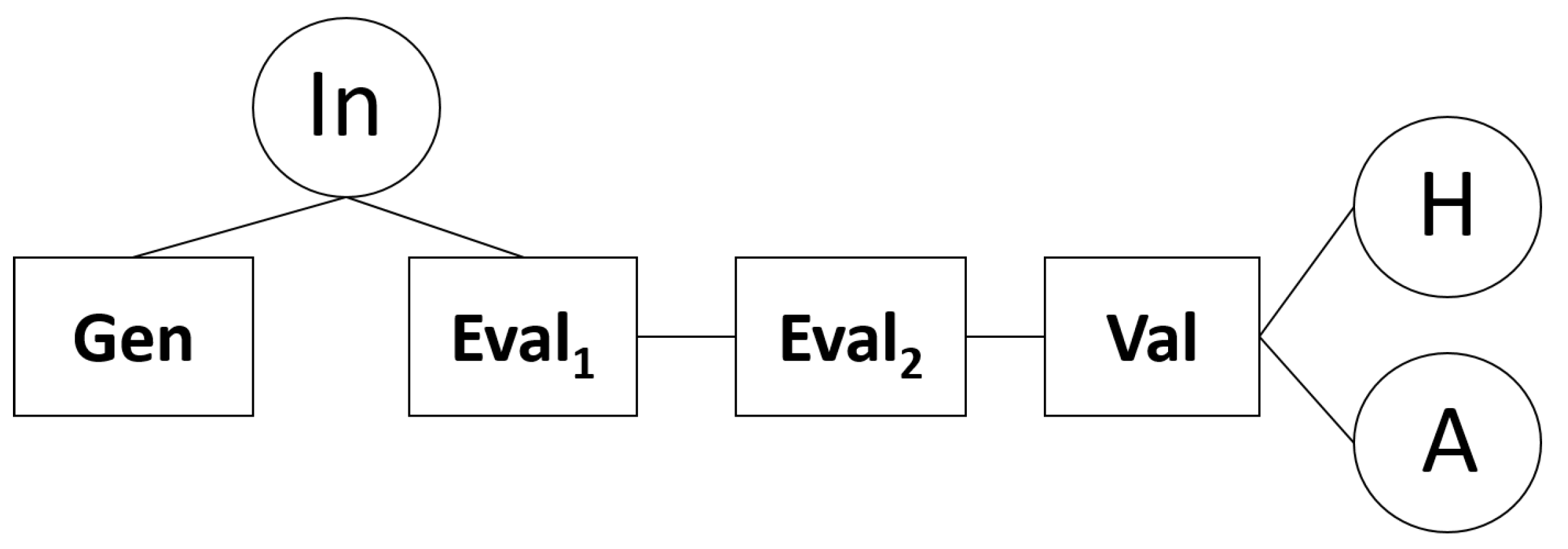
• The underlying graph G of our proposed $\mathsf{\Gamma }$ is depicted in the Figure 1. The nodes In, H and A are the input, halting and accept nodes, respectively, while the boxes Gen, ${\mathbf{Eval}}_{\mathbf{1}}$, ${\mathbf{Eval}}_{\mathbf{2}}$, Val are subnetworks representing the different stages or phases for $\mathsf{\Gamma }$ computation. In particular, the box Gen represents the subnetwork in charge of the combinatorial task for generating all pictures $\pi$ containing the different values for the indeterminates $x_1,x_2,\dots x_n$ for each input picture. Also, both boxes ${\mathbf{Eval}}_{\mathbf{1}}$ and ${\mathbf{Eval}}_{\mathbf{2}}$ represent the subnetworks for the phases of evaluation. The former represents the subnetwork that computes the evaluation of the $n+1$ row of a given picture, namely, the evaluation of the terms $p_i^{\left(k\right)}{x}_i$, while the latter represents the subnetwork that computes the evaluation of the first n-rows of a given picture, namely, the evaluation of the terms $p_{i,j}^{\left(k\right)}{x}_i{x}_j$. Finally, the box Val represents the subnetwork in charge of the phase for selecting the pictures that satisfy the Equation (4). Detailed description for each subnetwork as well as the $In,H$ and A nodes are introduced in the Section 4.1, Section 4.2, Section 4.3, Section 4.4, Section 4.5. In addition, the internals for each subnetwork are given in the Figure 2, Figure 3, Figure 4 and Figure 5.
• With regards to the mapping R for $\mathsf{\Gamma }$, it is specified for each node in the

  Table 2. Internals of the In node and nodes of the subnetwork $\mathbf{Gen}$.

  Node	M	$\mathit{\alpha }$	$\mathit{\beta }$	S
  In	$\{c_0\to c_0^{\prime }\}$	$[2n(n+1),2n^2(n+1)]$	$\{\downarrow \}$	$\{C\cup C^{″}\},$
  		$\{-n\left(2^{(n+1)}\right)\}$		$\{C^{\prime }\cup \{■\}\cup \left\{\ddot{k}\right\}\cup B\}$
  $X_i^0,1\le i\le n$	$\{x_i\to \underline{x_i},c_i\to c_i^{\prime },c_0^{\prime }\to c_0\}$	$[-(2^{(n+1)}+1),-1],$	$\{+\}$	$\{X\cup \dot{X}\cup \ddot{X}\cup \left\{{\mathsf{\$}}^{\prime }\right\}\},$
  		$\{-n\left(2^{(n+1)}\right)\}$		$\{C^{\prime }\cup \{■\}\cup \left\{\ddot{k}\right\}\cup B\}$
  $X_i^1,1\le i\le n$	$\{x_i\to \overline{x_i},c_i\to c_i^{\prime },c_0^{\prime }\to c_0\}$	$[-(2^{(n+1)}+1),-1],$	$\{+\}$	$\{X\cup \dot{X}\cup \ddot{X}\cup \left\{{\mathsf{\$}}^{\prime }\right\}\},$
  		$\{-n\left(2^{(n+1)}\right)\}$		$\{C^{\prime }\cup \{■\}\cup \left\{\ddot{k}\right\}\cup B\}$

  ,

  Table 3. Internals of the nodes of the subnetwork ${\mathbf{Eval}}_{\mathbf{1}}$.

  Node	M	$\mathit{\alpha }$	$\mathit{\beta }$	S
  G	$\left\{\mathrm{mask}\right\}$	$[-2n(n+1)\left(2^{(n+1)}\right),-n\left(2^{(n+1)}\right)]$	$\{\downarrow \}$	$\{C^{\prime }\cup \{■\}\cup \left\{\ddot{k}\right\}\cup B\},$
  				$\left\{\right\{⧫\}\cup \{\mathsf{\$}\left\}\right\}$
  L	$\{\mathsf{\$}\to ■\}$	$[2n^2(n+2),\infty ),$	$\{+\}$	$\left\{\right\{⧫\}\cup \{\mathsf{\$}\left\}\right\}$,
  		$[-n^2\left(2^{(n+1)}\right),-n\left(2^{(n+1)}\right)]$		$\{C^{\prime }\cup \{■\}\cup \left\{\ddot{k}\right\}\cup B\},$
  Q	$\left\{\mathrm{mask}\right\}$	$[0,n(2n+1\left)\right],$	$\{\downarrow \}$	$\{\underline{X}\cup \underline{X^{\prime }}\cup \overline{X}\cup \overline{X^{\prime }}\cup \left\{1\right\}\cup \left\{0\right\}\}$
  		$[-n^2\left(2^{(n+1)}\right),-n\left(2^{(n+1)}\right)]$		$\{C^{\prime }\cup \{■\}\cup \left\{\ddot{k}\right\}\cup B\},$
  $\underline{X_i^0},1\le i\le n$	$\{\underline{x_i}\to \dot{x_i}\}$	$[-2n(n+1)\left(2^{(n+1)}\right),-n\left(2^{(n+1)}\right)],$	$\{\downarrow \}$	$\{C^{\prime }\cup \{■\}\cup \left\{\ddot{k}\right\}\cup B\},$
  		$\{-1\}$		$\{X\cup \dot{X}\cup \ddot{X}\cup \left\{{\mathsf{\$}}^{\prime }\right\}\}$
  $\underline{X_i^{\prime 0}},1\le i\le n$	$\{\overline{p_i^{\left(k\right)}}\to 0,\underline{p_i^{\left(k\right)}}\to 0,$	$[-(2^{(n+1)}+1),-1]$	$\{\downarrow \}$	$\{X\cup \dot{X}\cup \ddot{X}\cup \left\{{\mathsf{\$}}^{\prime }\right\}\},$
  	$\dot{x_i}\to \underline{x_i^{\prime }}\}$			$\{\underline{X}\cup \underline{X}\cup \overline{X}\cup \overline{X^{\prime }}\cup \left\{1\right\}\cup \left\{0\right\}\}$
  $\overline{X_i^1},1\le i\le n$	$\{\overline{p_i^{\left(k\right)}}\to ⧫,\underline{p_i^{\left(k\right)}}\to {\mathsf{\$}}^{\prime },$	$[-2n(n+1)\left(2^{(n+1)}\right),-n\left(2^{(n+1)}\right)],$	$\{\downarrow \}$	$\{C^{\prime }\cup \{■\}\cup \left\{\ddot{k}\right\}\cup B\},$
  	$\overline{x_i}\to \dot{x}\}$	$\left\{2n^2(n+2)\right\}$		$\left\{\right\{⧫\}\cup \{\mathsf{\$}\left\}\right\}$
  $\underline{X_i^{\prime 1}},1\le i\le n$	$\{\dot{x}\to \overline{x_i^{\prime }},{\mathsf{\$}}^{\prime }\to 0\}$	$[-(2^{(n+1)}+1),-1],$	$\{\downarrow \}$	$\{X\cup \dot{X}\cup \ddot{X}\cup \left\{{\mathsf{\$}}^{\prime }\right\}\}$,
  		$[-n^2\left(2^{(n+1)}\right),-n\left(2^{(n+1)}\right)]$		$\{C^{\prime }\cup \{■\}\cup \left\{\ddot{k}\right\}\cup B\}$
  $\overline{X_i^{\prime 1}},1\le i\le n$	$\{\dot{x}\to \overline{x_i^{\prime }},⧫\to 1\}$	$[2n^2(n+2),\infty ),$	$\{\downarrow \}$	$\left\{\right\{⧫\}\cup \{\mathsf{\$}\left\}\right\}$
  		$[-n^2\left(2^{(n+1)}\right),-n\left(2^{(n+1)}\right)]$		$\{C^{\prime }\cup \{■\}\cup \left\{\ddot{k}\right\}\cup B\}$

  ,

  Table 4. Internals of the nodes of the subnetwork ${\mathbf{Eval}}_{\mathbf{2}}$.

  Node	M	$\mathit{\alpha }$	$\mathit{\beta }$	S
  $U_1$	$\left\{\mathrm{unmask}\right\}$	$[2n^2(n+2),\infty ),$	$\{\downarrow \}$	$\left\{\right\{⧫\}\cup \{\mathsf{\$}\left\}\right\}$
  		$\{-2(n+1)\left(2^{(n+1)}\right)\}$		$\{C^{\prime }\cup \{■\}\cup \left\{\ddot{k}\right\}\cup B\}$
  $F_1$	$\{c_0^{\prime }\to c_0^{″},{⊞}^k\to {⊠}^k\}$	$[-2n(n+1)\left(2^{(n+1)}\right),-n\left(2^{(n+1)}\right)],$	$\{\downarrow \}$	$\{C^{\prime }\cup \{■\}\cup \left\{\ddot{k}\right\}\cup B\}$
  	$1\le k\le m$	$\left\{2n\right(n+1\left)\right\}$		$\{C\cup C^{″}\}$
  $F_2$	$\{c_i^{″}\to c_{i+1}^{″},■\to \mathsf{\$}\}$	$[2n^2(n+2),\infty ),$	$\{+\}$	$\left\{\right\{⧫\}\cup \{\mathsf{\$}\left\}\right\}$
  	$\mathrm{for} \mathrm{all} 0\le i\le n$	$\{-\left(n^2\right)\left(2^{(n+1))}\right\}$		$\{C^{\prime }\cup \{■\}\cup \left\{\ddot{k}\right\}\cup B\}$
  M	$\left\{\mathrm{mask}\right\}$	$[2n^2(n+2),\infty ),$	$\{\to \}$	$\left\{\right\{⧫\}\cup \{\mathsf{\$}\left\}\right\}$
  		$\{-n\left(2^{(n+1)}\right)\}$		$\{C^{\prime }\cup \{■\}\cup \left\{\ddot{k}\right\}\cup B\}$
  $A_1^0$	$\{\underline{p_{i,j}^{\left(k\right)}}\to 0,\underline{x_i}\to {\mathsf{\$}}^{\prime },\overline{x_i}\to {\mathsf{\$}}^{\prime }\}$	$[2n^2(n+2),\infty ),$	$\{\uparrow \}$	$\left\{\right\{⧫\}\cup \{\mathsf{\$}\left\}\right\},$
  	for all $1\le i,j\le n$	$\{-2\}$		$\{X\cup \dot{X}\cup \ddot{X}\cup \left\{{\mathsf{\$}}^{\prime }\right\}\}$
  $\overline{A_i^1}$	$\{\overline{p_{i,j}^{\left(k\right)}}\to 1,$$\overline{x_i}\to {\mathsf{\$}}^{\prime },\underline{x_i}\to \mathsf{\$}\}$	$[2n^2(n+2),\infty ),$	$\{\uparrow \}$	$\left\{\right\{⧫\}\cup \{\mathsf{\$}\left\}\right\},$
  	for all $1\le i,j\le n$	$\{-2\}$		$\{X\cup \dot{X}\cup \ddot{X}\cup \left\{{\mathsf{\$}}^{\prime }\right\}\}$
  $\underline{A_i^1}$	$\{\overline{p_{i,j}^{\left(k\right)}}\to 0,$$\overline{x_i}\to \mathsf{\$},\underline{x_i}\to {\mathsf{\$}}^{\prime }\}$	$[2n^2(n+2),\infty ),$	$\{\uparrow \}$	$\left\{\right\{⧫\}\cup \{\mathsf{\$}\left\}\right\},$
  	for all $1\le i,j\le n$	$[-2,-1]$		$\{X\cup \dot{X}\cup \ddot{X}\cup \left\{{\mathsf{\$}}^{\prime }\right\}\}$
  $F_3$	$\{c_i^{\prime }\to \ddot{c_i},{\mathsf{\$}}^{\prime }\to \mathsf{\$}\}$	$[-(2^{(n+1)}+1),-1]$	$\{+\}$	$\{X\cup \dot{X}\cup \ddot{X}\cup \left\{{\mathsf{\$}}^{\prime }\right\}\}$,
  	for all $1\le i\le n$			$\{C^{\prime }\cup \{■\}\cup \left\{\ddot{k}\right\}\cup B\}$
  $U_2$	$\left\{\mathrm{unmask}\right\}$	$[2n^2(n+2),\infty ),$	$\{\to \}$	$\left\{\right\{⧫\}\cup \{\mathsf{\$}\left\}\right\},$
  		$\{-n\left(2^{(n+1)}\right)\}$		$\{C^{\prime }\cup \{■\}\cup \left\{\ddot{k}\right\}\cup B\}$
  $M_1$	$\left\{\mathrm{mask}\right\}$	$\{-4mn(n+1)\left(2^{(n+1)}\right)\}$	$\{\leftarrow \}$	$\{\ddot{C}\cup B^{\prime }\cup \left\{c_0^0\right\}\cup \left\{c_0^1\right\}\},$
  				$\left\{\right\{⧫\}\cup \{\mathsf{\$}\left\}\right\}$
  $F_5$	$\{\ddot{c_n}\to c_n^{\prime },{⊠}^i\to {⊞}^k\}$	$\{-4mn(n+1)\left(2^{(n+1)}\right)\}$	$\{\to \}$	$\{\ddot{C}\cup B^{\prime }\cup \left\{c_0^0\right\}\cup \left\{c_0^1\right\}\},$
  	$1\le k\le m$			$\left\{\right\{⧫\}\cup \{\mathsf{\$}\left\}\right\}$
  $F_6$	$\{\mathsf{\$}\to \ddot{k}\}$	$[2n^2(n+2),\infty ),$	$\{\uparrow \}$	$\left\{\right\{⧫\}\cup \{\mathsf{\$}\left\}\right\}$,
  		$[-(n+2)\left(2^{(n+1)}\right),-3n\left(2^{(n+1)}\right)]$		$\{C^{\prime }\cup \{■\}\cup \left\{\ddot{k}\right\}\cup B\}$
  $M_2$	$\left\{\mathrm{mask}\right\}$	$[2n^2(n+2),\infty ),$	$\{\uparrow \}$	$\left\{\right\{⧫\}\cup \{\mathsf{\$}\left\}\right\}$
  		$\{-3n\left(2^{(n+1)}\right)\}$		$\{C^{\prime }\cup \{■\}\cup \left\{\ddot{k}\right\}\cup B\}$
  $U_3$	$\left\{\mathrm{unmask}\right\}$	$[0,n(2n+1\left)\right],$	$\{\leftarrow \}$	$\{\underline{X}\cup \underline{X^{\prime }}\cup \overline{X}\cup \overline{X^{\prime }}\cup \left\{1\right\}\cup \left\{0\right\}\}$
  		$\left\{2n{(n+1)}^2\right\}$		$\{C\cup C^{″}\}$
  $F_7$	$\{\ddot{c_i}\to c_i^{\prime }, \mathrm{for} \mathrm{all} 1\le i\le n\}$	$[2n^2(n+2),\infty ),$	$\{\downarrow \}$	$\left\{\right\{⧫\}\cup \{\mathsf{\$}\left\}\right\}$
  		$\{-n(n+2)\left(2^{(n+1)}\right)\}$		$\{C^{\prime }\cup \{■\}\cup \left\{\ddot{k}\right\}\cup B\}$
  $S_1$	$\left\{\mathrm{unmask}\right\}$	$[2n^2(n+2),\infty ),$	$\{\uparrow \}$	$\left\{\right\{⧫\}\cup \{\mathsf{\$}\left\}\right\}$
  		$\{-(2n+1)n\left(2^{(n+1)}\right)\}$		$\{C^{\prime }\cup \{■\}\cup \left\{\ddot{k}\right\}\cup B\}$
  $S_2$	$\left\{\mathrm{unmask}\right\}$	$[2n^2(n+2),\infty ),$	$\{\leftarrow \}$	$\left\{\right\{⧫\}\cup \{\mathsf{\$}\left\}\right\}$
  		$\left\{2n\right(n+1\left)\right\}$		$\{C\cup C^{\prime \prime }\}$

  and

  Table 5. Internals of the nodes of the subnetwork $\mathbf{Val}$.

  Node	M	$\mathit{\alpha }$	$\mathit{\beta }$	S
  W	$\{\overline{x_i^{\prime }}\to \ddot{x_i},\underline{x_i^{\prime }}\to \dot{x},$	$[2n^2(n+2),\infty ),$	$\{+\}$	$\left\{\right\{⧫\}\cup \{\mathsf{\$}\left\}\right\},$
  	$\ddot{k}\to \mathsf{\$}\},1\le i\le n$	$\{-n(n+1)\left(2^{(n+1)}\right)\}$		$\{C^{\prime }\cup \{■\}\cup \left\{\ddot{k}\right\}\cup B\}$
  $V_0$	$\{\overline{p_0^{\left(k\right)}}\to 1,\underline{p_0^{\left(k\right)}}\to 0\}$	$\{[-2n(n+1)\left(2^{(n+1)}\right),-n\left(2^{(n+1)}\right)],$	$\{+\}$	$\{C^{\prime }\cup \{■\}\cup \left\{\ddot{k}\right\}\cup B\},$
  	$1\le k\le m$	$\{1,3,5,7.\dots (2n+1\left)\right\}$		$\{\underline{X}\cup \underline{X^{\prime }}\cup \overline{X}\cup \overline{X^{\prime }}\cup \left\{1\right\}\cup \left\{0\right\}\}$
  $V_1$	$\{\overline{p_0^{\left(k\right)}}\to 1,\underline{p_0^{\left(k\right)}}\to 0\}$	$\{[-2n(n+1)\left(2^{(n+1)}\right),-n\left(2^{(n+1)}\right)],$	$\{+\}$	$\{C^{\prime }\cup \{■\}\cup \left\{\ddot{k}\right\}\cup B\},$
  	$1\le k\le m$	$\{0,2,4,\dots 2n\}$		$\{\underline{X}\cup \underline{X^{\prime }}\cup \overline{X}\cup \overline{X^{\prime }}\cup \left\{1\right\}\cup \left\{0\right\}\}$
  $V_0^{\prime }$	$\{c_0^{\prime \prime }\to c_0^1,c_1^{\prime }\to \ddot{c_1}$,	$[2n^2(n+2),\infty ),$	$\{\downarrow \}$	$\left\{\right\{⧫\}\cup \{\mathsf{\$}\left\}\right\},$
  	$c_i^{\prime }\to \mathsf{\$}\},2\le i\le n$	$\{-n(n+1)\left(2^{(n+1)}\right)\}$		$\{C^{\prime }\cup \{■\}\cup \left\{\ddot{k}\right\}\cup B\}$
  $V_1^{\prime }$	$\{c_0^{\prime \prime }\to c_0^0,c_1^{\prime }\to {\ddot{c}}_1,$	$[2n^2(n+2),\infty ),$	$\{\downarrow \}$	$\left\{\right\{⧫\}\cup \{\mathsf{\$}\left\}\right\},$
  	$c_i^{\prime }\to \mathsf{\$}\},\forall 2\le i\le n$	$\{-n(n+1)\left(2^{(n+1)}\right)\}$		$\{C^{\prime }\cup \{■\}\cup \left\{\ddot{k}\right\}\cup B\}$
  $V_2^i,$	$\{c_1^{\prime }\to R_i$},	$[2n^2(n+2),\infty ),$	$\{+\}$	$\left\{\right\{⧫\}\cup \{\mathsf{\$}\left\}\right\},$
  $0\le i<2^n$	$1\le i<2^n$	$\left\{2^i\right\}$		$\{X\cup \dot{X}\cup \ddot{X}\cup \left\{{\mathsf{\$}}^{\prime }\right\}\}$
  H	$\{\ddot{x_i}\to \overline{x_i},\dot{x_i}\to \underline{x_i}\}$,	$[-(2^{(n+1)}+1),-1]$	$\{+\}$	$\{X\cup \dot{X}\cup \ddot{X}\cup \left\{{\mathsf{\$}}^{\prime }\right\}\},$
  	$1\le i\le n$			$\left\{\right\{⧫\}\cup \{\mathsf{\$}\left\}\right\}$
  A	$\{c_0^0\to 0\}$	$[2n^2(n+2),\infty )$	$\{\downarrow \}$	$\left\{\right\{⧫\}\cup \{\mathsf{\$}\left\}\right\}$

  .
• With regards to the action mapping $\beta$ for $\mathsf{\Gamma }$, it is specified for each node in the Table 2, Table 3, Table 4 and Table 5.
• The mapping function $\rho$ is defined as follows:
  • $\rho (\underline{X}\cup \underline{X^{\prime }}\cup \overline{X}\cup \overline{X^{\prime }}\cup \left\{1\right\}\cup \left\{0\right\})=[0,n(2n+1)]$
  • $\rho (C\cup C^{″})=[2n(n+1),2n^2(n+1)]$
  • $\rho (\{⧫\}\cup \{\mathsf{\$}\})=[2n^2(n+2),\infty )$
  • $\rho (X\cup \dot{X}\cup \ddot{X}\cup \left\{{\mathsf{\$}}^{\prime }\right\})=[-(2^{(n+1)}+1),-1]$
  • $\rho (C^{\prime }\cup \{■\}\cup \left\{\ddot{k}\right\}\cup B)=[-2n(n+1)\left(2^{(n+1)}\right),-n\left(2^{(n+1)}\right)]$
  • $\rho (\ddot{C}\cup B^{\prime }\cup \left\{c_0^0\right\}\cup \left\{c_0^1\right\})=\{-4mn(n+1)\left(2^{(n+1)}\right)\}$
  We assume that any symbol in U not appearing in the previous mapping has an empty interval for evaluation since it is not relevant for the proposed algorithm.
• The function $\phi$ is defined as follows:
  • $\phi \left(\overline{p_i^{\left(k\right)}}\right)=\phi \left(\overline{p_{i,j}^{\left(k\right)}}\right)=\phi \left(\overline{p_0^{\left(k\right)}}\right)=\phi \left(\overline{x_i}\right)=\phi \left(1\right)=\phi \left(\overline{x_i^{\prime }}\right)=1$, for all $1\le k\le m,1\le i,j\le n$
  • $\phi \left(x_i\right)=\phi \left(\dot{x_i}\right)=\phi \left({\mathsf{\$}}^{\prime }\right)=-1$, for all $1\le i\le n$
  • $\phi \left(\underline{p_i^{\left(k\right)}}\right)=\phi \left(\underline{p_{i,j}^{\left(k\right)}}\right)=\phi \left(\underline{p_0^{\left(k\right)}}\right)=\phi \left(\underline{x_i}\right)=\phi \left(\underline{x_i^{\prime }}\right)=\phi \left(0\right)=0$, for all $1\le k\le m,0\le i,j\le n$
  • $\phi \left(\ddot{x_i}\right)=-\left(2^{(i-1)}\right)$, for all $1\le i\le n$
  • $\phi \left(c_i\right)=\phi \left(c_i^{″}\right)=2n(n+1)$, for all $0\le i\le n$
  • $\phi \left({⊞}^k\right)=\phi \left(c_i^{\prime }\right)=\phi \left(\ddot{k}\right)=\phi (■)=-n\left(2^{(n+1)}\right)$, for all $1\le k\le m,0\le i\le n$
  • $\phi (⧫)=\phi (\mathsf{\$})=2n^2(n+2)$
  • $\phi \left(\ddot{c_i}\right)=\phi \left({⊠}^k\right)=\phi \left(c_0^0\right)=\phi \left(c_0^1\right)=-2kn(n+1)\left(2^{(n+1)}\right)$, for all $1\le i\le n,1\le k\le m$
  We remark that the values for elements in P are given as input values.

4.1. The Node in

By default, in the initial configuration, the node In holds the input picture coding the instance of the problem to solve. For our network $\mathsf{\Gamma }$, the node In holds the input pictures representing each polynomial $P^{\left(1\right)}\left(\mathbf{x}\right),P^{\left(2\right)}\left(\mathbf{x}\right),\dots ,P^{\left(m\right)}\left(\mathbf{x}\right)$. In addition, this node serves like a both receptor and transmitter of the pictures processed by subnetwork $\mathbf{Gen}$. For this reason, this node only has a substitution rule that changes one control symbol by other one. In particular, while the subnetwork $\mathbf{Gen}$ is generating configurations, i.e., pictures with the corresponding symbols assigned to each indeterminate, these are allowed to pass to the ${\mathbf{Eval}}_{\mathbf{1}}$ subnetwork by the In node for further processing. This node’s internals are shown in Table 2.

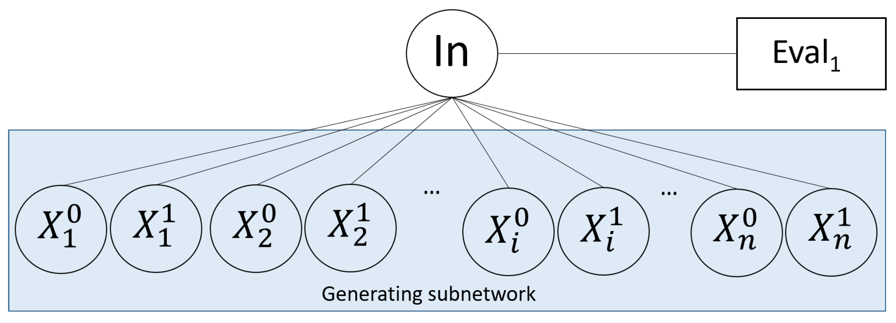
4.2. Generating Subnetwork

The subnetwork $\mathbf{Gen}$ represents the generating phase, namely, the phase in charge of generating $m·2^n$ configurations for the initial pictures ${\pi }^1,{\pi }^2,{\pi }^3,\dots {\pi }^m$ encoding an RMQE instance. In particular, this subnetwork replaces each $x_i$ for a symbol $\overline{x_i}$ or $\underline{x_i}$, which represents the value 1 or 0 respectively, and hence generates $2^n$ configurations for each initial picture ${\pi }^k$. The graphical representation of the underlying subgraph for subnetwork $\mathbf{Gen}$ is depicted in the Figure 2.

According to the Figure 2, each indeterminate $x_i$ is represented by two nodes, namely, $X_i^0$ and $X_i^1$. Concretely, the node $X_i^0$ replaces all occurrences of symbol $x_i$ for the symbol $\underline{x_i}$ (which represents 0). On the other hand, the node $X_i^1$ replaces all occurrences of symbol $x_i$ for one symbol $\overline{x_i}$ (which represents the value 1). After n processing steps, the subnetwork $\mathbf{Gen}$ will have modified all $x_i$ symbols and generated $2^n$ configurations for each initial picture ${\pi }^k$. These configurations will be collected by the In node. The internals of each node $X_i^1,X_i^0,1\le i\le n$ in this subnetwork are defined in the Table 2.

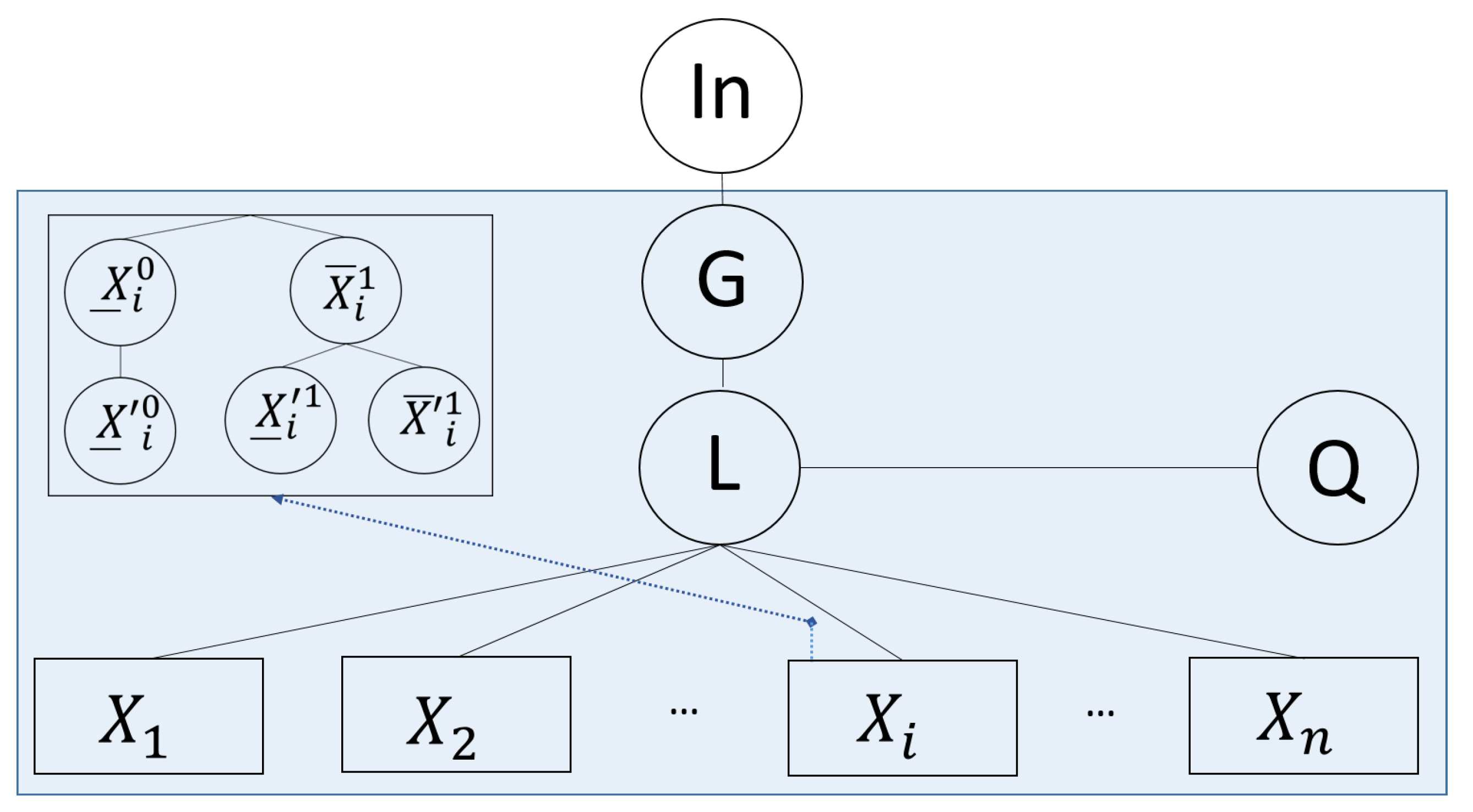
4.3. Linear-Evaluating Subnetwork

The aim of this subnetwork is to evaluate AND operations for each pair of symbols $p_i^{\left(k\right)}{x}_i$ with $1\le i\le n$, which are encoded at the row $n+1$ of each picture. The graph representing this subnetwork is depicted in the Figure 3.

This subnetwork starts off with the node G receiving pictures from the node $In$. The received pictures are then processed by the node G, by masking the two last rows (at indexes $(n+2)$ and $(n+3)$) from them. This makes each processed picture’s last visible row be the row that contains the terms $p_i^{\left(k\right)}{x}_i$ (i.e., the $n-1$ row). This row is what will then be processed by other nodes in this subnetwork, by applying on it substitution rules with the $\beta$ mode ↓.

The node L serves as a control node to keep the traceability of the substitution of each pair $p_i^{\left(k\right)}{x}_i$ done by the subnetwork $X_i$ depicted in the Figure 3 (the internals of these boxes can be seen in the rectangle at left-upper corner). In a similar way as the subnetwork $\mathbf{Gen}$ operates, the nodes $\underline{X_i^0}$ and $\overline{X_i^1}$ replace all occurrences of symbols $\underline{x_i}$ and $\overline{x_i}$ for an intermediary symbol in the set $\dot{X}$. With them, this subnetwork is able to evaluate whether the result of the AND operation for the pair $p_i^{\left(k\right)}{x}_i$ is 0 or 1 through the evaluation sets defined in the nodes $\underline{X_i^{\prime 0}}$ and $\overline{X_i^{\prime 1}}$, respectively. In these nodes, the symbols belonging to the set $P_L$ are substituted by the symbols either $\underline{x_i^{\prime }}$ or $\overline{x_i^{\prime }}$ according to the result from the AND operation (representing 0 and 1, respectively). Concretely, in the node $\overline{X_i^1}$, the symbols representing the $p_i^{\left(k\right)}$ values are substituted by trash symbols either ${\mathsf{\$}}^{\prime }$ or ⧫. Subsequently, the nodes $\overline{X_i^{\prime 1}}$ and $\underline{X_i^1}$ let pass only the pictures which evaluation represents 1 or 0, respectively. Then, they substitute the trash symbols for the specific result (1 or 0). Therefore, the result of the evaluation has been assigned to the place for the $p_i^{\left(k\right)}$ symbols at the picture. The processing for L and nodes represented in the boxes $X_i$ is repeated until all terms $p_i^{\left(k\right)}{x}_i$ in the pictures have been substituted, with the valid resulting pictures leaving the node L and entering the node Q. Finally, the node Q masks the recently evaluated row for all received pictures making only the first n rows visible, i.e., the rows that encode the terms the $p_{i,j}^{\left(k\right)}{x}_i{x}_j$. In this way, the pictures are prepared for the following phase (subnetwork ${\mathbf{Eval}}_{\mathbf{2}}$), which evaluates the quadratic terms. The internals of each node in this subnetwork ${\mathbf{Eval}}_{\mathbf{1}}$ are defined in the Table 3.

4.4. Quadratic-Evaluating Subnetwork

This subnetwork is responsible for evaluating each term $p_{i,j}^{\left(k\right)}{x}_i{x}_j$ in the pictures. The result from evaluating the AND operation between each one these three terms will be represented by the substitution of the $p_{i,j}^{\left(k\right)}$ symbols by a symbol 0 or 1 (depending of the result). Similarly at the subnetwork ${\mathbf{Eval}}_{\mathbf{1}}$, the symbols $\underline{x_i}\mid \overline{x_i}$ are replaced by the trash symbols $ or ${\mathsf{\$}}^{\prime }$. The Figure 4 depicts the graph of this subnetwork. The internals of each node in this subnetwork are defined in the Table 4.

The processing of this subnetwork starts off with the node $U_1$ receiving all pictures from the node Q. Then, this node unmasks all invisible rows such that it makes the last rows visible. More specifically, the node $U_1$ unmasks the rows at indexes $(n+1)$,$(n+2)$ and $(n+3)$ in each received picture. After that, the processed pictures are allowed to move to the node $F_1$, which substitutes the control symbol $c_0^{\prime }$ and the symbol ${⊞}^k$ in each picture for the symbols $c_0^{″}$ and ${⊠}^k$, respectively. Note that this node only does this substitution once and it is only for controlling the internal processing.

After this substitution is carried out, the process for evaluating each row containing the terms $p_{i,j}^{\left(k\right)}{x}_i{x}_j$, $1\le i\le j\le n$ starts such that each term is evaluated one at time. The node $F_2$ is responsible for keeping track the evaluation of each row. Specifically, this node starts with the substitution of the symbol $c_0^{″}$ for $c_1^{″}$ in order to indicate that the row 1 will be evaluated subsequently. In addition, this node substitutes all symbols ■ for the trash symbol $, because they are no longer needed.

The next time this node receive pictures from node $F_7$, it can substitute the symbol again and so on until all rows are evaluated. The node M is able to mask all columns from the rightmost column to the column containing the $x_j$ (exclusive) symbol of the current $p_{i,j}^{\left(k\right)}{x}_i{x}_j$ to be evaluated (this is controlled by means of the $c_i^{\prime }$ symbol place at this same column). With this masking process, $\mathsf{\Gamma }$ makes visible only the current three terms $p_{i,j}^{\left(k\right)}{x}_i{x}_j$ at the first visible row. Subsequently, the operation AND is calculated for these three symbols in a similar way as it is processed for the subnetwork ${\mathbf{Eval}}_{\mathbf{1}}$ (in the boxes $X_i$). More concretely, this evaluation is done by the nodes $A_i^0,\underline{A_i^1}$ and $\overline{A_i^1}$. Then, the node $F_3$ substitutes the $c_i^{\prime }$ for ${\ddot{c}}_i$ in order to identify that the current quadratic term was evaluated. In addition, this node substitutes the ${\mathsf{\$}}^{\prime }$ symbol for the original one. Note that the result of the AND operation is encoded at the place in which the symbol $p_{i,j}^{\left(k\right)}$ was placed. In order to carry out the evaluation for the rest of the $p_{i,j}^{\left(k\right)}{x}_i{x}_j$ terms in the current row, the nodes $U_2$ and $M_1$ unmask the rightmost three columns and mask the current three visible columns, respectively. $M_1$ is connected with the nodes $A_i^0,\underline{A_i^1}$ and $\overline{A_i^1}$ and it allows that the process for evaluating each $p_{i,j}^{\left(k\right)}{x}_i{x}_j$ term is repeated until all of them are evaluated. When it occurs, the pictures from node $F_3$ migrate to the node $F_5$ and it makes the other branch of the subnetwork will be processed.

Given that the last control symbol substituted was $c_n^{\prime }$ by $\ddot{c_n}$, the pictures can enter to the node $F_5$. Then, this node returns the symbols $\ddot{c_n}$ to their original one ($c_n^{\prime }$). Similarly, this node substitutes the symbols ${⊠}^k$ by their original ones. After that, the pictures migrate to the node $F_6$ and this node substitutes one symbol $ for a $\ddot{k}$ in order to indicate that the current row was just evaluated. Then, the pictures enter to $M_2$ and the current row is masked. Subsequently, the node $U_3$ unmasks all masked columns to the left. The processing for this branch finishes when the node $F_7$ substitutes all $\ddot{c}$ symbols for their original ones in the set $C^{\prime }$. With these substitutions, $\mathsf{\Gamma }$ is able to evaluate the next visible row and hence, the pictures migrate to the $F_2$ node in order to repeat the processing of the next row. When the pictures do not contain $p_{i,j}^{\left(k\right)}{x}_i{x}_j$ symbols, then they migrate from the node $F_2$ to the node $S_1$. Note that all pictures with the symbol $\ddot{k}$ are allowed into the node $S_1$. Finally, the nodes $S_1$ and $S_2$ are responsible for unmasking all hidden rows and columns in order to promote them for the next phase.

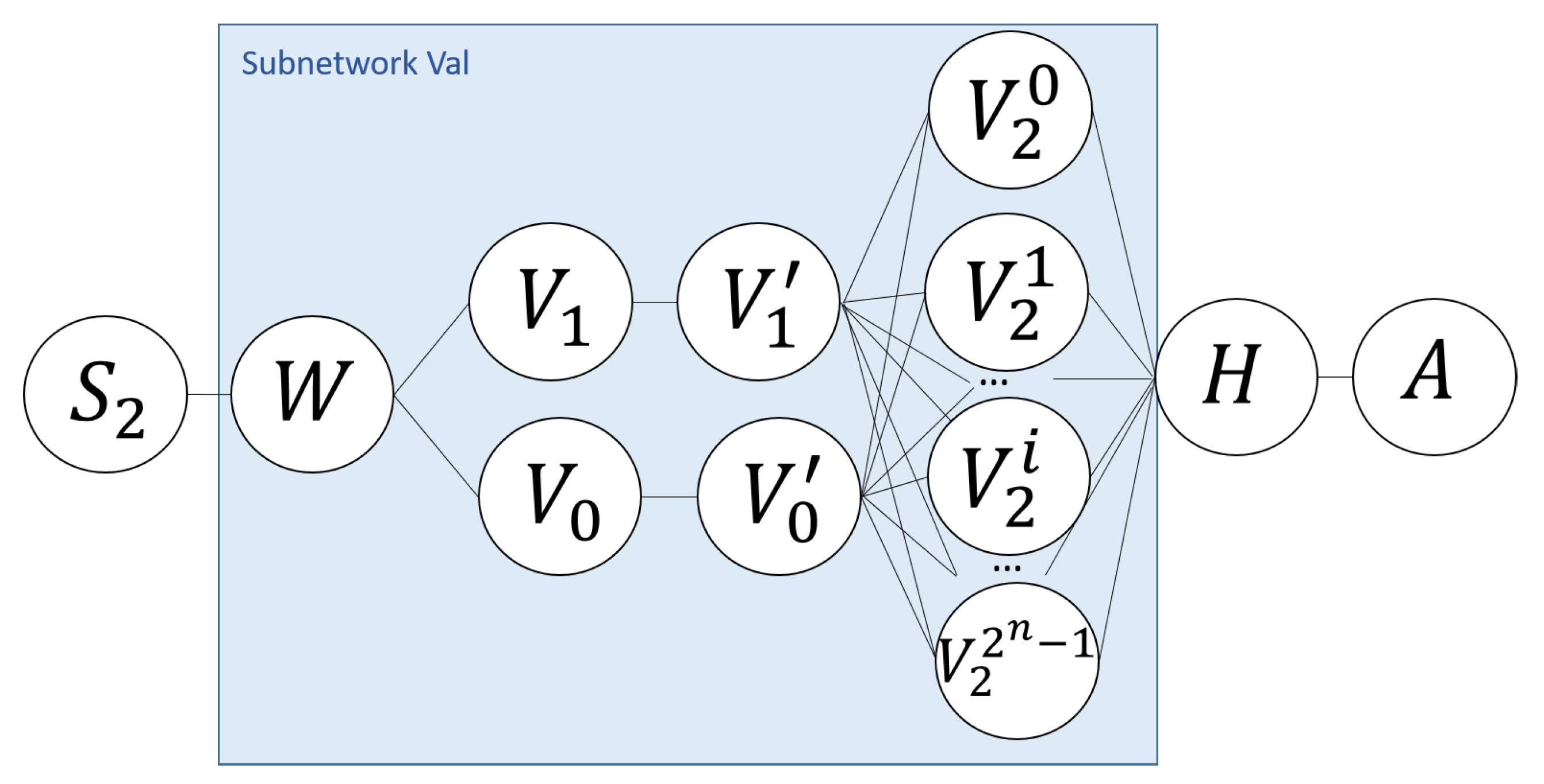
4.5. Validation Subnetwork

The goal of this subnetwork is twofold. First, this subnetwork calculates the final value for each picture, e.g., the evaluation to the polynomial that the picture represents. More specifically, this subnetwork computes the resulting value from each $P^{\left(i\right)}$ (i.e., 0 or 1), for all $1\le i\le m$, after performing XOR operations between the terms that compose the picture (summation of all them). This result will be stored as a value for the control symbol $c_0$ at the last row in the pictures. Second, this subnetwork groups all the pictures sharing the same values for the indeterminates $x_1,x_2,\dots x_n$. This grouping will allow to obtain the solutions for the problem, that is, to find vectors $\widehat{x}$ satisfying Equation (4). The values for each $x_i$ remains represented by the symbols belonging to $\underline{X^{\prime }}$ or $\overline{X^{\prime }}$ placed into the row n (0 or 1, respectively). The Figure 5 depicts the graph of this subnetwork.

Concretely, the nodes $V_1,V_0,V_1^{\prime }$ and $V_0^{\prime }$ performs a XOR operation with the values placed in rows from one to n and replace the control symbol $c_0$ with the result obtained from performing the XOR operation, i.e., by substituting the symbol $c_0$ by other control symbol $c_0^0$ if the result of XOR operation is 0 or $c_0^1$ otherwise. The nodes $V_2^i$, $0\le i<2^n$, group all pictures belonging to each possible combination of n values assigned to the indeterminates. In particular, each configuration is mapped to an integer in the range $[0,2^n-1]$. Previously, the node W has substituted all symbols in the sets $\underline{X^{\prime }}$ and $\overline{X^{\prime }}$ for their corresponding symbols in the sets $\dot{X}$ and $\ddot{X}$, respectively. It is necessary in order to evaluate each configuration filtering each picture according to the value obtained by nodes $V_2^i,0\le i<2^n$. These nodes substitutes the control symbol $c_1$ for a control symbol $R_i,0\le i\le 2^n-1$, where the index i represents the number of configuration. Finally, the node $Halt$ substitutes all symbols belonging to the sets $\dot{X}$ and $\ddot{X}$ for the original ones and the node $Accept$ collects all pictures representing the solution of the input instance. The internals of each node in this subnetwork are defined in the following Table 5.

4.6. Discussion

Lemma 1.

The NPPES Γ defined in Section 4 computes a solution for the RMQE problem.

Proof of Lemma 1.

At the beginning of the computation, $\mathsf{\Gamma }$ contains the set of pictures $\mathsf{\Pi }=\{{\pi }^{\left(1\right)},{\pi }^{\left(2\right)},\dots ,{\pi }^{\left(m\right)}\}$ encoding the polynomials to be evaluated (all of them in the node $In$). Thus, the initial configuration is defined by $C_0\left(In\right)=\mathsf{\Pi }$ and $C_0\left(x\right)=\varnothing ,\forall x\in X_G\backslash \left\{In\right\}$. 25A0 $\mathsf{\Gamma }$ consist of the initial pictures (with the $c_0$ symbol substituted by $c_0^{\prime }$) for all $X_i^0,X_i^1$, $1\le i\le n$ represented in the Figure 2. After n processing steps, the node $In$ has collected $m·2^n$ pictures. Note that for each initial picture $\pi \in \mathsf{\Pi }$, the subnetwork $\mathbf{Gen}$ generates a picture for each possible $n—$tuple of values to the indeterminates $x_1,x_2,\dots x_n$ in $\pi$. Therefore, it generates $m·2^n$ pictures that are collected by the node $In$ and are then sent out to the subnetwork ${\mathbf{Eval}}_{\mathbf{1}}$, more concretely to the node G. This node masks the three last rows in all received pictures and then sends the pictures out to the node L, which includes one new trash symbol indicating the first step to evaluate the terms placed in the row n, namely $p_i^{\left(k\right)}{x}_i$, for all $1\le i\le n,1\le k\le m$.

Note that the nodes $\underline{X_i^0},\underline{X_i^{\prime 0}}$ evaluate, in two processing steps, whether each term is 0. At the same processing steps, the $\overline{X_i^0},\overline{X_i^{\prime 0}}$ nodes evaluate whether each term is 1. These evaluations are done by applying simple substitution rules. After n processing steps, each picture will have all $p_i^{\left(k\right)}{x}_i$ terms evaluated and be collected by the node L. All pictures then migrate to the Q node, which masks the row containing the recently evaluated terms (last row) within a processing step. Then, the pictures are sent out to the subnetwork ${\mathbf{Eval}}_{\mathbf{2}}$, more precisely to the node $U_1$. This node makes all masked rows in each received picture visible through two processing steps. Note that $F_1$ is a control node which performs its task once, then it performs one processing step. $F_2$ controls the rows being evaluated by the subnetwork, starting from the first row by substituting one symbol $c_i^{\prime }$ and n symbols ■ using n processing steps. The nodes $M,M_1,F_3,U_2,A_1^0,\underline{A_i^1},\overline{A_i^1}$ evaluate each term $p_{i,j}^{\left(k\right)}{x}_i{x}_j$ in each corresponding row of a picture, by making the three columns occupied by each term visible and then performing an AND operation with the corresponding values. When all terms are evaluated, the hidden columns are made visible again and a mechanism to indicate that this row was evaluated is used. Then, these nodes perform n times their respective steps.

The nodes $F_5,F_6,F_7,M_2$ and $U_3$ make the just-evaluated row invisible, mark the index of the evaluated row (substituting the respective symbol in $C^{\prime }$ and preparing the pictures for the evaluation of the next row). After the evaluation of the possible occurrences of the $p_{i,j}^{\left(k\right)}{x}_i{x}_j$ terms, the node $S_1$ and subsequently $S_2$ collect all evaluated pictures and return the masked rows to the visible state after perform n and $n-3$ processing steps, respectively. Then $S_2$ contains a set of pictures encoding each and every admissible evaluation of each polynomial in the Equation (3). However, at this stage, we need to organize all pictures by classes, where each groups pictures of each polynomial for one of the $2^n$$n—$tuple of values that can be assigned to the indeterminates, and then determine which classes satisfy the Equation (4), if any (if a class has m pictures then the corresponding $n—$tuple is a solution).

The node W performs n processing steps in order to do all substitutions. $V_0$ and $V_1$ substitutes the independent term in the $n+1$ row of a picture for the corresponding symbol for all pictures at the same processing step. In addition, these nodes let can pass to the nodes $V_0^{\prime }$ and $V_1^{\prime }$ only the pictures with evaluation of all symbols 1 being wither odd or even, respectively. $V_0^{\prime }$ and $V_1^{\prime }$ nodes substitute control symbols at the last row in the same processing step. The nodes $V_2^i$ group the pictures according to each possible $n—$tuple of values for the indeterminates that satisfy Equation (4), via marking the picture with an $R_i$ symbol, where the index i represents the $i_{th}$$n—$tuple of values, at same processing step. The transition of H to A is immediate: H returns the symbols of the vector to the original ones and A puts the final result of the evaluation in the control symbol $c_0^0$. Each one of these two nodes perform one processing step. Finally, the node A collects the pictures containing the solution for the given instance. □

Therefore, as a consequence of this result, we obtained the following theorem:

Theorem 1.

The RMQE problem as it was defined in Section 3 can be solved by a NPPES Γ in time $O\left(n^2\right)$.

Proof of Theorem 1.

Following the identical conditions as we have mentioned before, the processing steps in $\mathsf{\Gamma }$ are:

• Node In: $n+1$ steps
• Subnetwork $\mathbf{Gen}$: n steps performed by $X_i^0$,$X_i^1$, $1\le i\le n,$ nodes.
• Subnetwork ${\mathbf{Eval}}_{\mathbf{1}}$: $3n+5$ steps performed as follows:

  −

  Node G: 2 steps

  −

  Node L: $(n+1)$ steps

  −

  Node Q: 2 steps

  −

  Nodes $\underline{X_i^0}$,$\overline{X_i^1}$, $1\le i\le n$: n steps

  −

  Nodes $\underline{X_i^{{}^{\prime }0}}$, $\underline{X_i^{{}^{\prime }1}}$, $\overline{X_i^{{}^{\prime }1}}$, $1\le i\le n$: n steps

• Subnetwork ${\mathbf{Eval}}_{\mathbf{2}}$: $3n(n+3)$ steps performed as follows:

  −

  Node $U_1$: 2 steps.

  −

  Node $F_1$: 1 step.

  −

  Nodes: $F_2,F_3,F_4,F_5,F_6,M_2,F_7$: $7n$ steps (1 processing step performed by every node)

  −

  Nodes $M_1,U_2$: $6n$ steps ($3n$ processing steps performed by every node)

  −

  Nodes $M,U_3$: at most $n(n-3)$ steps for each of these nodes, then $2n(n-3)$

  −

  Nodes $A_1^0,\overline{A_i^1}$ and $\underline{A_i^1}$: at most n processing steps for each n row, then, $n^2$ steps

  −

  Node $S_1$: n steps

  −

  Node $S_2$: $n-3$ steps

• Subnetwork $\mathbf{Val}$: $n+3$ steps performed as follows:

  −

  Node W: n processing steps

  −

  Nodes $V_1,V_0$, 1 step

  −

  Nodes $V_1^{\prime },V_0^{\prime }$, 1 step

  −

  Nodes $V_2^i,1\le i\le n$, 1 step

• Nodes H and A, 1 step every node, then, 2 steps.

Therefore, the total number of processing steps is not more than $3n^2+15n+11$. Note that, if a given instance of the problem has k solutions, with $k\ge 0$, then $\mathsf{\Gamma }$ finds the k $n—$tuples of values for the indeterminates that are solutions for the given instance. Consequently, the overall time for solving an instance of the RMQE problem, as it is defined in Equation (4), is $O\left(n^2\right)$. □

We remark that the proposed network $\mathsf{\Gamma }$ seems to have a significant size in terms of number of nodes. This can be seen as an aspect to be improved; however, note that this construction allows us to control the exponential growth of the generated strings in any moment. In addition, we obtain a viable solution in an acceptable computation time given the complexity of the problem we are dealing with. Also, $\mathsf{\Gamma }$ sieves the correct pictures in an early identification step, minimizing the unnecessary copies. Additionally, note that other NBP models do not give such flexibility when the problem needs to meet integer constraints. Consequently, NPPES opens up an interesting perspective to fill this gap. Another important reason to support the solution we presented here is that, given the high maturity achieved by the ultra-scalable computing platforms, since this facilities deploying distributed algorithms in a reasonable way [16], our proposed solution might be deployed by using any hardware/software solution as those reported in [30], without requiring any modification (re-structuring of nodes, rules, mechanism to workload distribution between computational units or so on). That is to say, we potentially may put our solution to run on workers or parallel computing units in any scalable software or hardware platform without re-defining the proposed algorithm, because our distribution of nodes would be more suitable to reallocate parallel processing units within a real computing platform.

5. Conclusions and Final Remarks

We have introduced a solver for the RMQE problem that is based on NPPES and runs in quadratic time, suggesting that the NPPES model can be employed to cope with hard complex problems in which numerical evaluation has an essential role. In this context, the extended model is able to deal with a new variety of hard problems because of the model’s new features, in particular its filtering strategy makes the selection of correct pictures easier compared to the previous model. Additionally, the model exhibits efficiency and uses up less resources than similar bio-inspired models facing similar hard problems. To the best of our knowledge, this is the first time in which an NBP model is used to propose a solver for the RMQE problem. Also this solver demonstrates the computational power that may be achieved by employing bio-inspired computational models, since existing non-bio-inspired solutions run in exponential time for specific $n,m$ input values. Furthermore, our proposed solution for the RMQE problem opens an interesting opportunity to propose new solvers for these complex problems, bringing about real computing solutions with a reasonable computing time (which can be understood as “efficient time”).

In previous works [14,31], it is stated that NPEP solutions need an adaptation for allowing the deployment on computational platforms for massive distributed processing. Moreover, this adaptation must preserve the solution’s complexity in order to achieve practical solutions to real problems on big data computing platforms (which is extensible to any solution using similar models computing pictures instead of strings). In this context, the proposed solution here does not require any adaptation to be deployed in massively parallel and distributed computing platforms, and therefore, we avoid the previously commented drawbacks when these algorithms are deployed in practical scenarios.

Our results additionally suggest that the NPPES model may be more simple than other models working on pictures or strings for tackling hard optimization problems with numerical evaluations. We thus think this model shows features worthy of further investigation, both from a theoretical approach and from a practical point of view. With respect to the latter, we think studying the limits of software and hardware implementations to attack complex problems with big data computing platforms deserves effort and attention. Additionally, researching into the suitability of extending this model to reinforce it for other related high-processing problems also is interesting. Finally, we shall return to these topics in a forthcoming work.