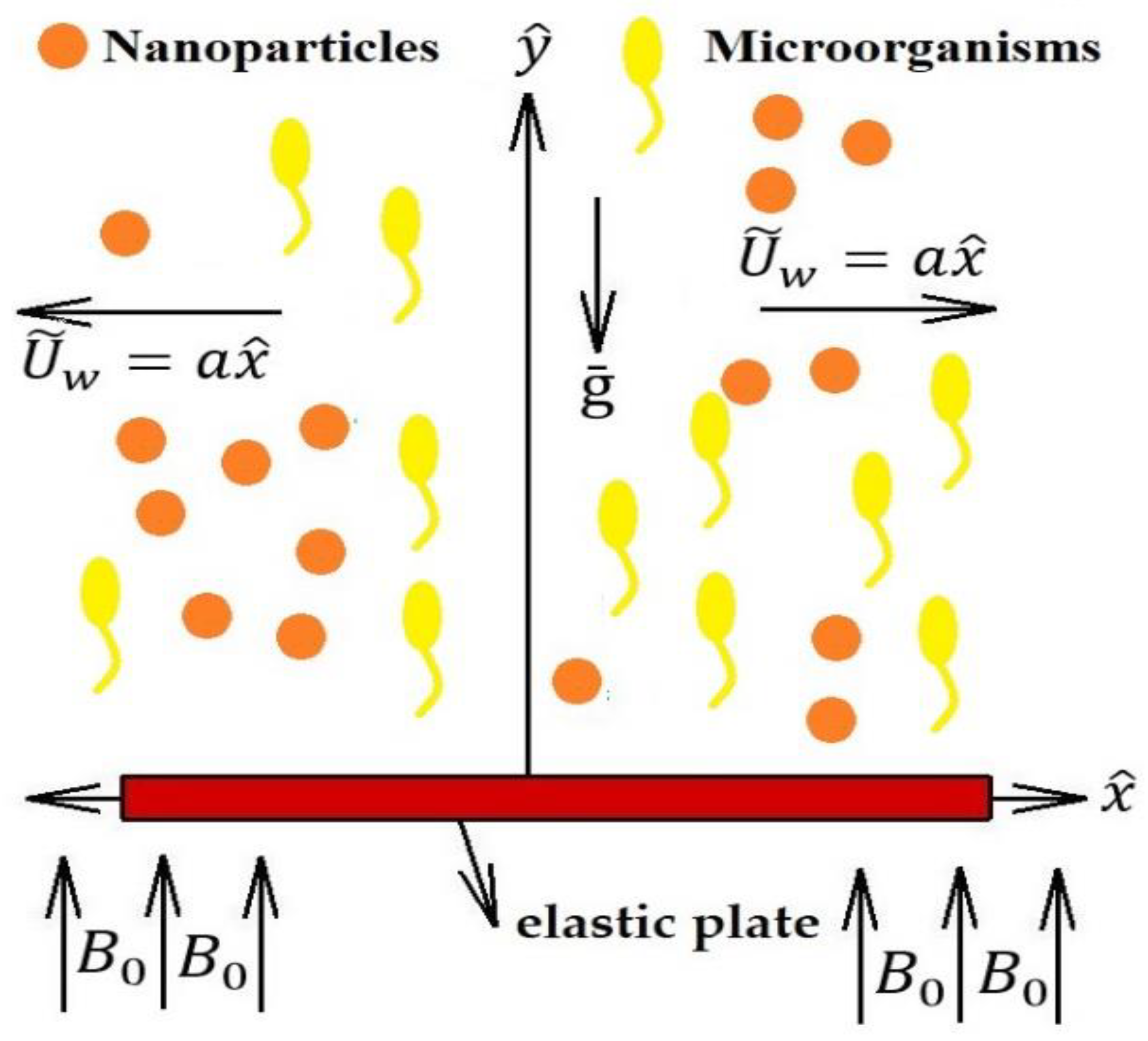
Numerical Investigation on the Swimming of Gyrotactic Microorganisms in Nanofluids through Porous Medium over a Stretched Surface

Abstract

In this article, the effects of swimming gyrotactic microorganisms for magnetohydrodynamics nanofluid using Darcy law are investigated. The numerical results of nonlinear coupled mathematical model are obtained by means of Successive Local Linearization Method. This technique is based on a simple notion of the decoupling systems of equations utilizing the linearization of the unknown functions sequentially according to the order of classifying the system of governing equations. The linearized equations, that developed a sequence of linear differential equations along with variable coefficients, were solved by employing the Chebyshev spectral collocation method. The convergence speed of the SLLM technique can be willingly upgraded by successive applying over relaxation method. The comparison of current study with available published literature has been made for the validation of obtained results. It is found that the reported numerical method is in perfect accord with the said similar methods. The results are displayed through tables and graphs.

1. Introduction

The problems associated with the boundary layer mechanism and heat transfer flow through stretched subsurface have been eminently accepted through analysts as long as the presence in structures of enormous industrial and technologically significance. Few of the advanced spreading applications encompass the designing of plastic layers and copper cables, glass-fiber fabricating, food and polymer refining, geothermal power extraction, liquefying-spinning productions, polymer melting, hot roll glass blasting, in the formation of the final product, in the textile industry, and other abundant utilities. Sakiadis [1] performed the developing effort in the area of boundary layer flow on a continued stable subsurface flowing with steady velocities. Later, Crane [2] was the earliest who extended the conception for boundary layer flow through stretchable surfaces. He examined a closed mode result for the Newtonian fluid flow past a flat stretched subsurface. Banks [3] investigated the similarity solutions for the boundary layer flow through a stretched wall with non-Newtonian fluid. Gupta and Gupta [4] broadened the investigated idea by Crane with the heat and mass transfer past a stretchable surface, along with the influence of suction/blowing. Bujurke et al. [5] discussed the heat transfer phenomenon past a boundary layer, along with interval heat generation. Cortell [6] analyzed the viscous fluid flow numerically with heat transfer on a nonlinearly stretchable subsurface. Shahzad et al. [7] developed the exact solutions of the axisymmetric flow with heat transfer for MHD viscous fluid on a nonlinearly radial pervious stretched surface. Hayat et al. [8] explored the MHD axisymmetric flow for third-grade fluid with heat transfer over stretchable sheets. Shateyi and Makinde [9] recorded the heat transfer analysis for a viscous, electrically conducting fluid flow through a radial stretched and convectively heated disk. Khan et al. [10] discussed the mix convection heat transfer to Sisko fluid past radial stretchable surface together with the influence of convection boundary conditions, thermal radiation, and viscous dissipative terms. Since it is known that the standard of the final product relies on the rate of heat transfer as acknowledged, hence the nanofluids have a higher thermal conductivity of the nanoparticles utilized to enhance the rate for heat transfer [11,12]. For this purpose, distinct techniques are adopted to raise the thermal conductivity of the fluids by providing suspension of nano/micro or large-sized particles into liquids. An inventive approach to enhance the heat transfer rate is performed by utilizing nano-scale particles into the governing fluid by Choi et al. [13]. They recorded that by adding a tiny extent (less than 1% by volume) of the nanoparticles to regular heat transfer fluids enhanced the thermal conductivity for the fluids up to almost 4-times and higher. Kuznetsov and Nield [14] discussed the natural convection into a nanofluid through a vertical surface, along with the impact of thermophoresis and the Brownian-motion. Noghrehabadadi et al. [15] explored the heat transfer of nanofluids past a stretched subsurface with supposing of thermal convectively boundary conditions and partial slip. Zaraki et al. [16] analyzed the influence of the various shapes, sizes, and types of nanoparticles, and base-fluid flowing and heat transferring properties for a naturally convective boundary layer.

The investigations for magnetohydrodynamics have significant utilities, and also uses in cooling of nuclear reactors by the induction flow meter and liquid, depending on the capability variation into the fluid in order normal to the flow and the magnetic field. Ferdows et al. [17] explored the problem for magnetized nanofluid mixed convective flow past an exponential stretched plate. Bidin and Nazar [18] discussed the numerical investigation for boundary layer flow through an exponential stretchable surface, along with thermal emission. Khan et al. [19] studied the unsteady boundary layer flow for a nanofluid on a horizontal stretched plate together with the impact of MHD and thermal radiation. Mabood et al. [20] studied the MHD boundary layer nanofluid flowing with the influence of heat transfer and viscous dissipation through a nonlinear stretched surface. Freidoonimehr et al. [21] studied the magnetized stagnation point flow through a stretched/shrinkable surface alongside the impact of chemical reactions and heat absorption/generation. It is conclusive to mention here that Makinde and Animasaun [22] investigated an admirable work related to magnetized nanofluid flow alongside bioconvection with quartic autocatalysis chemical reaction. The results show that for a fixed numeric of a magnetic parameter, the local skin friction further develops at larger thickened parametric value, whereas the rate for local heat transfer turns lesser at a high-temperature parametric value past an uppermost subsurface of a paraboloid of an uprising. The possible developments and/or applications of the presented analysis to the same topic and to other related topics can be seen in [23,24,25,26,27,28,29,30,31,32,33,34,35,36,37,38].

The terminology bioconvection was first acknowledged in an article belonging to James Henry Platt to bring about other researchers to this consideration side towards the physics of streaming forms noticed in impenetrable fashions of free-floating microorganisms. In light of Platt [39], the movement of polygonal forms in impenetrable fashions of Tetrahymena (i.e., ciliate and flagellate), such as Benard cells, though not by thermo-convection. Since, it is well-known that the presence of microorganisms (bacteria) are everywhere, and it is illustrious evidence that a large number of bacteria may be accidentally suffered and sometimes can be shot down when periodically bared to a higher temperature, conflicting that thermophile is an organism that usually can be seen in different heated territories on the earth. The self-impelled motile microorganisms brought enhancement in the density of the base fluid in a peculiar way to produce a bioconvection kind of stream. Basing on the cause of propulsion, the motile microorganisms perhaps categorized into various types of microorganisms, counting oxytactic or chemotaxis, gyrotactic microorganisms, and negate gravitaxis. Contrasting the motile microorganisms, the nanoparticles are not self-propelled, and their migration is through the Brownian-motion and thermophoresis impact inward nanofluid. Ghorai and Hill [40] farther elucidated that bioconvection is a known terminology to indicate the phenomena for impromptu arrangement in the suspension of microorganisms, such as algae and bacteria. Bioconvection also can be explained as the macroscopic convective movement of fluid as a result of the density gradient, and is brought about by the jointly floating of motile microorganisms. Alike naturally convective process, bioconvection is induced by versatile stratification density. Kuznetsov and Avramenko [41] interpreted that when bioconvection takes place, it boosts mingling and diminishes the establishing of the particles that are decisive in medicine utilities. Khan and Makinde [42] examined nanofluid bioconvection caused by gyrotactic microorganisms and noticed that the self-propelled motile microorganisms enhance the density of the base-fluid as floating/swimming in a specific manner. Recently, Raees et al. [43] interpreted that bioconvection into nanofluids has enormous contributions in Colibri micro-volumes spectrometer and benefits the stability in nanofluids. Natural convection with double-diffusive effects over a boundary layer nanofluid flow has been examined by Kuznetsov and Nield [44]. Nonetheless, if the stimulators past the subsurface are more imperative and associate to the bulk-fluid, comprising 36 nm nanoparticles and gyrotactic microorganism, alike chemical backlash could be examined by applying the conception of homogeneous–heterogeneous quartic strategy. Sivaraj et al. [45] have discussed the gyrotactic microorganisms on the mechanism of 29 nm copper water nanofluids propagated through a horizontal surface of paraboloid. Amirsom et al. [46] have considered the movement of microorganisms on a magnetized nanofluid in the presence of second order slip conditions via bvp4c computational scheme. Waqas et al. [47,48] used a shooting method to discuss the propagation of nanoparticles and gyrotactic microorganisms through a stretching surface with magnetic and porous effects using non-Newtonian fluid models. A few other inquiries on gyrotactic microorganisms can be read here [49,50,51].

The impulsion of the current investigation is to explore the impact of a non-uniform magnetic field on the conduct of water suspension comprising nanoparticles and motile gyrotactic microorganisms flowing through a stretchable permeable sheet by employing Successive Local Linearization Method (SLLM) with the combination of Chebyshev spectral linearization method [52] not yet available in the existing literature. The governing flow equations and the boundary conditions were brought towards nonlinear ordinary differential equations by utilizing the similarity variable transformations, and are than solved numerically by spectral approach.

2. Mathematical Modeling

A two-dimensional, steady, incompressible viscous and electrically conducting nanofluid flow, comprising gyrotactic microorganisms through a stretched porous sheet by Darcy-Forchheimer relation is considered. It is also assumed that the flow field is under the effect of a varying magnetic field of strength $B\left(x\right) = B_0\left(\widehat{x}\right)$. The sheet is stretched vertically with velocity ${\tilde{U}}_w = a\widehat{x}$, with positive constant $a$. The induced magnetic field is ignored because it is minimal in comparison to the extraneous magnetic field, as can be seen in Figure 1. The concentration ${\tilde{C}}_{w,}$ temperature ${\tilde{T}}_w,$ and densities for motile microorganisms are ${\tilde{N}}_w$ and ${\tilde{N}}_{\infty }$ past the stretched subsurface are considered constant and bigger than the ambient concentration ${\tilde{C}}_{\infty }$, temperature ${\tilde{T}}_{\infty },$ respectively. It is further presumed that nanoparticles are not affecting the direction and velocity of microorganisms, and both the nanoparticles and the base fluid are in local thermal stability state; and the nanoparticles, motile microorganisms, and the base-fluid are having the equivalent velocities. Hence, for a suchlike problem, the governing equations for continuity, momentum, nanoparticle concentration, thermal energy, and microorganisms can be written as

$$\frac{\partial \tilde{v}}{\partial \widehat{y}}+\frac{\partial \tilde{u}}{\partial \widehat{x}} = 0,$$

(1)

$$\begin{array}{cc}\hfill \tilde{u}\frac{\partial \tilde{u}}{\partial \widehat{x}}+\tilde{v}\frac{\partial \tilde{u}}{\partial \widehat{y}}+\sigma B_0^2\tilde{u} = & -\frac{\partial \tilde{p}}{\partial \widehat{x}}+{\nu }_f\left(\frac{{\partial }^2\tilde{u}}{\partial {\widehat{x}}^2}+\frac{{\partial }^2\tilde{u}}{\partial {\widehat{y}}^2}\right)+\overline{\mathrm{g}}\beta \left(1-{\tilde{C}}_{\infty }\right)\left(\tilde{T}-{\tilde{T}}_{\infty }\right)-\overline{\mathrm{g}}\left({\rho }_p-{\rho }_f\right)(\tilde{C}-\hfill \\ & {\tilde{C}}_{\infty })-\overline{\mathrm{g}}\gamma \left({\rho }_m-{\rho }_f\right)\left(\tilde{N}-{\tilde{N}}_{\infty }\right)-\frac{{\nu }_f}{k}\tilde{u},\hfill \end{array}$$

(2)

$$\frac{\partial \tilde{p}}{\partial \widehat{y}} = 0$$

(3)

$$\begin{array}{cc}\hfill \tilde{u}\frac{\partial \tilde{T}}{\partial \widehat{x}}+\tilde{v}\frac{\partial \tilde{T}}{\partial \widehat{y}} = & \overline{\alpha }\left[\frac{{\partial }^2\tilde{T}}{\partial {\widehat{x}}^2}+\frac{{\partial }^2\tilde{T}}{\partial {\widehat{y}}^2}\right]+\tilde{\tau }\left[D_B\frac{\partial \tilde{C}}{\partial \widehat{y}}\frac{\partial \tilde{T}}{\partial \widehat{y}}+\frac{D_T}{T_{\infty }}\left\{{\left(\frac{\partial \tilde{T}}{\partial \widehat{y}}\right)}^2+{\left(\frac{\partial \tilde{T}}{\partial \widehat{x}}\right)}^2\right\}\right]+\frac{{\mu }_f\overline{\alpha }}{k_t}{\left(\frac{\partial \tilde{u}}{\partial \widehat{y}}\right)}^2\hfill \\ & +\frac{\sigma \overline{\alpha }{B_0}^2}{k_t}{\tilde{u}}^2\hfill \end{array}$$

(4)

$$\tilde{u}\frac{\partial \tilde{C}}{\partial \widehat{x}}+\tilde{v}\frac{\partial \tilde{C}}{\partial \widehat{y}} = D_b\left[\frac{{\partial }^2\tilde{C}}{\partial {\widehat{x}}^2}+\frac{{\partial }^2\tilde{C}}{\partial {\widehat{y}}^2}\right]+\frac{D_T}{T_{\infty }}\left[\frac{{\partial }^2\tilde{T}}{\partial {\widehat{x}}^2}+\frac{{\partial }^2\tilde{T}}{\partial {\widehat{y}}^2}\right]$$

(5)

$$\tilde{u}\frac{\partial \tilde{N}}{\partial \widehat{x}}-D_M\left(\frac{{\partial }^2\tilde{N}}{\partial {\widehat{x}}^2}+\frac{{\partial }^2\tilde{N}}{\partial {\widehat{y}}^2}+2\frac{{\partial }^2\tilde{N}}{\partial \widehat{x}\partial \widehat{y}}\right)+\tilde{v}\frac{\partial \tilde{N}}{\partial \widehat{y}}+\frac{b{W}_C}{\left(\tilde{C}-{\tilde{C}}_{\infty }\right)}\left[\frac{\partial }{\partial \widehat{y}}\left(N\frac{\partial \tilde{C}}{\partial \widehat{y}}\right)+\frac{\partial }{\partial \widehat{x}}\left(\tilde{N}\frac{\partial \tilde{C}}{\partial \widehat{x}}\right)\right] = 0$$

(6)

Their respective boundary conditions can be read as

$$\tilde{u} = a\widehat{x}, \tilde{v} = 0,\tilde{T} = {\tilde{T}}_w, \tilde{C} = {\tilde{C}}_w,\tilde{N} = {\tilde{N}}_w \mathrm{at} \widehat{y} = 0$$

(7)

$$\tilde{u}\to 0, \tilde{C}\to {\tilde{C}}_{\infty },\tilde{v}\to 0, \tilde{T}\to {\tilde{T}}_{\infty }, \tilde{N}\to {\tilde{N}}_{\infty } \mathrm{as} \widehat{y}\to \infty$$

(8)

By cancelling Equation (3) from the momentum equations by cross-differentiation, only Equation (2) survives. In Equations (1)–(8), $\tilde{u}$ and $\tilde{v}$ are the velocity components for $\widehat{x}$ and $\widehat{y}$ directions correspondingly. Where $\tilde{T}$ is the temperature, $\tilde{C}$ is the concentration for nanoparticle,$\tilde{N}$ is the density for motile microorganism, $\tilde{p}$ is the pressure, ${\rho }_f$, ${\rho }_m, {\rho }_p$ are the densities of nanofluid, microorganisms, and nanoparticles, $D_b$, $D_m$, $D_T$ denote the Brownian-diffusion coefficient, diffusivity of microorganisms and thermophoresis-diffusion coefficient, $k$ the porosity parameter, $\sigma$, $k_t$ are the electrical and thermal conductivity for the fluid, $\gamma$ indicates the average volume for a microorganism, respectively. $\overline{\alpha } = k_t/\left(\rho c_p\right)$ is the thermal diffusivity, $b{W}_C$ are the constants, and the proportion of the effected heat capacitance of the nanoparticle to the base-fluid $\tilde{\tau } =\frac{{\left(\rho C\right)}_p}{{\left(\rho C\right)}_f},$ respectively, are the other parametric quantities.

Invoking the following transformation

$$\begin{array}{c}\hfill \tilde{u} = a\widehat{x}{g}^{\prime }\left(\eta \right), \tilde{v}= -\sqrt{a\nu }g\left(\eta \right), \eta = \sqrt{\frac{a}{\nu }} \widehat{y},\varphi \left(\eta \right) = \frac{\tilde{C}-{\tilde{C}}_{\infty }}{{\tilde{C}}_w-{\tilde{C}}_{\infty }},\\ \theta \left(\eta \right) = \frac{\tilde{T}-{\tilde{T}}_{\infty }}{{\tilde{T}}_w-{\tilde{T}}_{\infty }}, \Phi \left(\eta \right) = \frac{\tilde{N}-{\tilde{N}}_{\infty }}{{\tilde{N}}_w-{\tilde{N}}_{\infty }}.\end{array}\},$$

(9)

In Equations (1)–(8), the non-dimensional form of resulting equations, along with associated boundary conditions, can be written as

$$g^{‴}+g{g}^{″}-g^{\prime 2}-M{g}^{\prime }-{\beta }_D{g}^{\prime }+\frac{G_r}{R_e^2}\left(\theta -N_r\varphi -R_b\Phi \right) = 0$$

(10)

$$\frac{1}{P_r}{\theta }^{″}+{\theta }^{\prime }\left[g+N_b{\varphi }^{\prime }\right]+N_t\theta {\prime }^2+E_c\left\{{g″}^2+M{g}^{\prime 2}\right\} = 0$$

(11)

$${\varphi }^{″}+L_e {\varphi }^{\prime }g+\frac{N_t}{N_b}{\theta }^{″} = 0$$

(12)

$${\Phi }^{″}+L_{b}g{\Phi }^{\prime }- P_e\left(\left[\Phi +{\mathsf{\Omega }}_d\right]{\varphi }^{″}+{\varphi }^{\prime }{\Phi }^{\prime }\right) = 0$$

(13)

$$g\left(\eta \right) = 0,g^{\prime }\left(\eta \right) = 1,\theta \left(\eta \right) = \varphi \left(\eta \right) = \Phi \left(\eta \right) = 1, \mathrm{when} \eta = 0$$

(14)

$$g^{\prime }\left(\eta \right) = 0, \theta \left(\eta \right) = \varphi \left(\eta \right) = \Phi \left(\eta \right) = 0, \mathrm{when} \eta \to \infty$$

(15)

In which

$$\begin{array}{c}{\beta }_D = \frac{\nu }{a{\rho }_{f}k},M = \frac{\sigma {B_0}^2}{a{\rho }_f},\frac{G_r}{R_e^2}=\frac{\overline{\mathrm{g}}\beta \left(1-{\tilde{C}}_{\infty }\right)\left(\tilde{T}-{\tilde{T}}_{\infty }\right)}{a{\tilde{U}}_w},N_r = \frac{({\rho }_p-{\rho }_f)\left({\tilde{C}}_w-{\tilde{C}}_{\infty }\right)}{\beta {\rho }_f\left({\tilde{T}}_w-{\tilde{T}}_{\infty }\right)\left(1-{\tilde{C}}_{\infty }\right)},P_r = \frac{\nu }{\overline{\alpha }},R_b = \\ \frac{\gamma ({\rho }_m-{\rho }_f)\left({\tilde{N}}_w-{\tilde{N}}_{\infty }\right)}{\beta {\rho }_f\left({\tilde{T}}_w-{\tilde{T}}_{\infty }\right)\left(1-{\tilde{C}}_{\infty }\right)},N_T = \frac{\tilde{\tau }{D}_T\left({\tilde{T}}_w-{\tilde{T}}_{\infty }\right)}{\nu {\tilde{T}}_{\infty }},N_b = \frac{\tilde{\tau }{D}_B\left({\tilde{C}}_w-{\tilde{C}}_{\infty }\right)}{\nu },E_c = \frac{{{\tilde{U}}_w}^2}{c_p\left({\tilde{T}}_w-{\tilde{T}}_{\infty }\right)},L_e = \frac{\nu }{D_B},L_b =\\ \frac{\nu }{D_M},{\mathsf{\Omega }}_d = \frac{{\tilde{N}}_{\infty }}{\left({\tilde{N}}_w-{\tilde{N}}_{\infty }\right)},P_e =\frac{b{W}_C}{D_M},\end{array}$$

(16)

These parametric quantities are permeability parameter ${\beta }_D$, Hartmann number $M$, the local Richardson number $G_r/R_e^2$, the buoyancy proportion parameter $N_r$, Prandtl number $P_r$, the bioconvection Rayleigh number $R_b$, the thermophoresis parameter $N_t$, the Brownian motion parameter $N_b$, Eckert number $E_c$, the conventional Lewis number and the bioconvection Lewis number $L_e$ and $L_b$, the bioconvection Peclet number $P_e$, and ${\mathsf{\Omega }}_d$ is the concentration of the microorganisms variance parametric quantity, respectively.

The motile density number, Sherwood, and Nusselt number for the present flow in dimensionless form are:

$$\frac{N{u}_x}{R{e}_x^{1/2}} = -{\theta }^{\prime }\left(0\right),\frac{S{h}_x}{R{e}_x^{\frac{1}{2}}} = -{\varphi }^{\prime }\left(0\right), \frac{N{n}_x}{R{e}_x^{\frac{1}{2}}} = -{\Phi }^{\prime }\left(0\right),$$

(17)

where $R{e}_x = \frac{U_0\widehat{x}}{\nu },$ the local Reynolds number.

3. Numerical Solutions

3.1. Spectral Local Linearization Scheme

Let us having a system of differential equations $G=\left[g_1\left(\mathsf{\xi }\right),g_1\left(\mathsf{\xi }\right),\dots ,g_p\left(\mathsf{\xi }\right)\right]$ satisfying the system:

$${ℒ}_j+{Ñ}_j = {\mathscr{H}}_j, j = 1,2,\dots ,p,$$

(18)

where $p$ describes the number of differential equations, each ${\mathscr{H}}_j$ is a function of $\mathsf{\xi }ϵ\left[A,B\right]$ and ${ℒ}_j$, ${Ñ}_j$ are the linear and nonlinear components in the system, respectively.

Usually, the SLLM is an iterative approach to solve the differential equations, starts from an initial approximation $g_0,$ and then implements the SLLM successively, yielding the new approximations $g_1,g_2, \dots$, where $G_t = \left[g_{1,t},g_{2,t},\dots ,g_{p,t}\right]$ for each $t = 0,1,2$. When once linearized, the nonlinear components are ${Ñ}_j.$

For this intention, the $j$-th differential Equation (18) after the first $t+1$ iterations can be express as

$${{ℒ}_j|}_{t+1}+{{Ñ}_j|}_{t+1} = {\mathscr{H}}_j,$$

(19)

The nonlinear components can be linearized by using Taylor series

$${{Ñ}_j|}_{t+1} = {{Ñ}_j|}_t+\nabla {{Ñ}_j|}_t\left[V_{t+1}-V_t\right],$$

(20)

where $V_t$ is an n-tuple of $G_{j,t}$ and its differentials. Now using Equations (19) and (20) in Equation (18), it becomes

$${{ℒ}_j|}_{t+1}+\nabla {{Ñ}_j|}_t{V}_{t+1} = {\mathscr{H}}_j+\nabla {{Ñ}_j|}_t{V_t-{Ñ}_j|}_t.$$

(21)

3.2. Successive Local Linearization Method

For the implementation of Successive Local Linearization Method, first we have to reduce the order of Equation (24). To serve the purpose, a new transformation $g^{\prime } = h$, leads Equation (10) to Equation (13) into the following form:

$$h^{″}+g{h}^{\prime }-h^2-Mh-{\beta }_{D}h+\frac{G_r}{R_e^2}\left(\theta -N_r\varphi -R_b\Phi \right) = 0,$$

(22)

$$\frac{1}{P_r}{\theta }^{″}+{\theta }^{\prime }\left[g+N_b{\varphi }^{\prime }\right]+N_t\theta {\prime }^2+E_c\left\{h{\prime }^2+M{h}^2\right\} = 0,$$

(23)

$${\varphi }^{″}+L_e{\varphi }^{\prime }g+\frac{N_t}{N_b}{\theta }^{″} = 0,$$

(24)

$${\Phi }^{″}+L_{b}g{\Phi }^{\prime }-P_e\left\{\left[\Phi +{\mathsf{\Omega }}_d\right]{\varphi }^{″}+{\varphi }^{\prime }{\Phi }^{\prime }\right\} = 0.$$

(25)

Linearizing the non-linear term $h^2$ by applying Taylor series expansion can be written as

$${h^2}_{t+1}={h^2}_t+2h_t\left[h_{t+1}-h_t\right] = 2h_t{h}_{t+1}-{h^2}_t$$

(26)

where the component having subscripts $t$ and $t+1$ stand for current previous and current approximated values. When Equation (26) is placed in Equation (22), then the non-linear system by means of Gauss-Seidel relaxation method can be decoupled as:

$${g^{\prime }}_{t+1} = h_t$$

(27)

$${h^{″}}_{t+1}+g_t{h^{\prime }}_{t+1}-M{h}_{t+1}-{\beta }_D{h}_{t+1}-2h_t{h}_{t+1} = -{h^2}_t-\frac{G_r}{R_e^2}({\theta }_t-N_r{\varphi }_t-R_b{\Phi }_t)$$

(28)

$$\frac{1}{P_r}{{\theta }^{″}}_{t+1}+{{\theta }^{\prime }}_{t+1}[g_t+N_b{{\varphi }^{\prime }}_t]+N_t\theta {{\prime }^2}_{t+1} = -E_c\left\{h{\prime }^2{}_{t+1}+M{h^2}_{t+1}\right\}$$

(29)

$${{\varphi }^{″}}_{t+1}+L_e{g}_t{{\varphi }^{\prime }}_{t+1}+\frac{N_t}{N_b}{{\theta }^{″}}_{t+1} = 0$$

(30)

$${{\Phi }^{″}}_{t+1}+L_b{g}_t{{\Phi }^{\prime }}_{t+1}-P_e([{\Phi }_{t+1}+{\mathsf{\Omega }}_d]{{\varphi }^{″}}_{t+1}+{{\varphi }^{\prime }}_{t+1}{{\Phi }^{\prime }}_{t+1}) = 0$$

(31)

The corresponding boundary conditions become

$$g_{t+1}\left(0\right) = 0,h_{t+1}\left(0\right) = 1 = {\theta }_{t+1}\left(0\right) = {\varphi }_{t+1}\left(0\right) = {\Phi }_{t+1}\left(0\right),$$

(32)

$$h_{t+1}(\infty ) = 0 = {\theta }_{t+1}(\infty ) = {\varphi }_{t+1}(\infty ) = {\Phi }_{t+1}(\infty ),$$

(33)

Writing a compact expression of Equations (27)–(31) as follows

$${g^{\prime }}_{t+1} = d_{00}$$

(34)

$${h^{″}}_{t+1}+d_{11}{h^{\prime }}_{t+1}- d_{13}{h}_{t+1}-2h_t{h}_{t+1} = d_{1,t}$$

(35)

$$\frac{1}{P_r}{{\theta }^{″}}_{t+1}+d_{11}{{\theta }^{\prime }}_{t+1}+N_b {{\varphi }^{\prime }}_t{{\theta }^{\prime }}_{t+1}+N_t\theta {{\prime }^2}_{t+1} = d_{2,t}$$

(36)

$${{\varphi }^{″}}_{t+1}+d_{32}{{\varphi }^{\prime }}_{t+1}+\frac{N_t}{N_b}{{\theta }^{″}}_{t+1} = d_{3,t}$$

(37)

$${{\Phi }^{″}}_{t+1}+d_{42}{{\Phi }^{\prime }}_{t+1}-P_e\left\{\left[{\Phi }_{t+1}+{\mathsf{\Omega }}_d\right]{{\varphi }^{″}}_{t+1}+{{\varphi }^{\prime }}_{t+1}{{\Phi }^{\prime }}_{t+1}\right\} = d_{4,t}$$

(38)

where

$$\begin{array}{cc}\hfill {\mathit{d}}_{00} = {\mathit{h}}_{\mathit{t}},{\mathit{d}}_{11}& = {\mathit{g}}_{\mathit{t}},{\mathit{d}}_{12} = 2{\mathit{h}}_{\mathit{t}},{\mathit{d}}_{13} = \left[\mathit{M}+{\mathit{\beta }}_{\mathit{D}}\right],{\mathit{d}}_{1,\mathit{t}}\hfill \\ & = -{{\mathit{h}}^2}_{\mathit{t}}-\frac{{\mathit{G}}_{\mathit{r}}}{{\mathit{R}}_{\mathit{e}}^2}\left({\mathit{\theta }}_{\mathit{t}}-{\mathit{N}}_{\mathit{r}}{\mathit{\varphi }}_{\mathit{t}}-{\mathit{R}}_{\mathit{b}}{\mathit{\Phi }}_{\mathit{t}}\right)\hfill \end{array}$$

(39)

$${\mathit{d}}_{2,\mathit{t}}=-{\mathit{E}}_{\mathit{c}}\left({{{\mathit{h}}^{\prime }}^2}_{\mathit{t}+1}+\mathit{M}{{\mathit{h}}^2}_{\mathit{t}+1}\right),{\mathit{d}}_{32}={\mathit{L}}_{\mathit{e}}{\mathit{g}}_{\mathit{t}},{\mathit{d}}_{42}={\mathit{L}}_{\mathit{b}}{\mathit{g}}_{\mathit{t}},{\mathit{d}}_{3,\mathit{t}}={\mathit{d}}_{4,\mathit{t}}=0$$

(40)

Now, employing the Chebyshev spectral collocation method at the system of Equations (34)–(38), where the differentiation matrix $\mathit{D} = \frac{2}{l}\mathit{D}$ utilized to perform approximation for the derivatives of unknown variables in the above equations and our new system become

$$\mathit{D}{g}_{t+1} = h_{\mathit{t}}$$

(41)

$$\left\{{\mathit{D}}^2+diag\left[d_{11}\right]\mathit{D}-diag\left[d_{12}\right]\mathit{I}-d_{13}\mathit{I}\right\}{\mathit{H}}_{\mathit{t}+1}=d_{1,t}$$

(42)

$$\left\{\frac{1}{P_r}{\mathit{D}}^2+diag\left[d_{11}\right]\mathit{D}+N_{b}diag\left[{{\varphi }^{\prime }}_t\right]\mathit{D}+N_t{\mathit{D}}^2\right\}{\theta }_{t+1} = d_{2, t}$$

(43)

$$\left\{{\mathit{D}}^2+diag\left[d_{32}\right]\mathit{D}+\frac{N_t}{N_b}diag\left[{{\theta }^{″}}_{t+1}\right]\mathit{I}\right\}{\varphi }_{t+1} = d_{3,t}$$

(44)

$$\left\{\begin{array}{c}{\mathit{D}}^2+diag\left[d_{42}\right]\mathit{D}-P_e{\mathsf{\Omega }}_{d}diag\left[{{\varphi }^{″}}_{t+1}\right]\mathit{I}-P_{e}diag\left[{{\varphi }^{″}}_{t+1}\right]\mathit{I}\\ -diag\left[{{\varphi }^{\prime }}_{t+1}\right]\mathit{D}\end{array}\right\}{\Phi }_{t+1} = d_{4,t}$$

(45)

With their respective boundary conditions

$$g_{t+1}\left({\eta }_N\right) = 0,h_{t+1}\left({\eta }_N\right) = 1 = {\theta }_{t+1}\left({\eta }_N\right)={\varphi }_{t+1}\left({\eta }_N\right) = {\Phi }_{t+1}\left({\eta }_N\right)$$

(46)

$$h_{t+1}\left({\eta }_0\right) = 0 = {\theta }_{t+1}\left({\eta }_0\right) = {\varphi }_{t+1}\left({\eta }_0\right) ={\Phi }_{t+1}\left({\eta }_0\right),$$

(47)

The system can be expressed in a more simplified way as

$$B_1{g}_{t+1} = E_1$$

(48)

$$B_2{h}_{t+1} = E_2$$

(49)

$$B_3{\theta }_{t+1} = E_3$$

(50)

$$B_4{\varphi }_{t+1} = E_4$$

(51)

$$B_5{\varphi }_{t+1} = E_5$$

(52)

where

$${\mathit{B}}_1 =\mathit{D},{\mathit{E}}_1 = {\mathit{h}}_{\mathit{t}},$$

(53)

$${\mathit{B}}_2 = {\mathit{D}}^2+\mathit{d}\mathit{i}\mathit{a}\mathit{g}\left[{\mathit{d}}_{11}\right]\mathit{D}-\mathit{d}\mathit{i}\mathit{a}\mathit{g}\left[{\mathit{d}}_{12}\right]\mathit{I}-{\mathit{d}}_{13}\mathit{I},{\mathit{E}}_2={\mathit{d}}_{1,\mathit{t}},$$

(54)

$${\mathit{B}}_3 = \frac{1}{{\mathit{P}}_{\mathit{r}}}{\mathit{D}}^2+\mathit{d}\mathit{i}\mathit{a}\mathit{g}\left[{\mathit{d}}_{11}\right]\mathit{D}+{\mathit{N}}_{\mathit{b}}\mathit{d}\mathit{i}\mathit{a}\mathit{g}\left[{{\mathit{\varphi }}^{\prime }}_{\mathit{t}}\right]\mathit{D}+{\mathit{N}}_{\mathit{t}}{\mathit{D}}^2,{\mathit{E}}_3 = {\mathit{d}}_{2,\mathit{t}},$$

(55)

$${\mathit{B}}_4 = {\mathit{D}}^2+\mathit{d}\mathit{i}\mathit{a}\mathit{g}\left[{\mathit{d}}_{32}\right]\mathit{D}+\frac{{\mathit{N}}_{\mathit{t}}}{{\mathit{N}}_{\mathit{b}}}\mathit{d}\mathit{i}\mathit{a}\mathit{g}\left[{{\mathit{\theta }}^{″}}_{\mathit{t}+1}\right]\mathit{I},{\mathit{E}}_4 = {\mathit{d}}_{3,\mathit{t}},$$

(56)

$$\begin{array}{c}{\mathit{B}}_5 = {\mathit{D}}^2+\mathit{d}\mathit{i}\mathit{a}\mathit{g}\left[{\mathit{d}}_{42}\right]\mathit{D}-{\mathit{P}}_{\mathit{e}}{\Omega }_{\mathit{d}}\mathit{d}\mathit{i}\mathit{a}\mathit{g}\left[{{\mathit{\varphi }}^{″}}_{\mathit{t}+1}\right]\mathit{I}-{\mathit{P}}_{\mathit{e}}\mathit{d}\mathit{i}\mathit{a}\mathit{g}\left[{{\mathit{\varphi }}^{″}}_{\mathit{t}+\mathbf{1}}\right]\mathit{I}\\ -\mathit{d}\mathit{i}\mathit{a}\mathit{g}\left[{{\mathit{\varphi }}^{\prime }}_{\mathit{t}+1}\right]\mathit{D},{\mathit{E}}_5 = {\mathit{d}}_{4,t},\end{array},$$

(57)

$$\mathit{d}\mathit{i}\mathit{a}\mathit{g}\left[{\mathit{d}}_{\mathbf{11}}\right] = \left[\begin{array}{ccc}{\mathit{d}}_{\mathbf{11}}\left({\mathit{\eta }}_{\mathbf{0}}\right)& \cdots & \\ ⋮& \ddots & ⋮\\ & \cdots & {\mathit{d}}_{\mathbf{11}}\left({\mathit{\eta }}_{\mathit{N}}\right)\end{array}\right], \mathit{d}\mathit{i}\mathit{a}\mathit{g}\left[{\mathit{d}}_{\mathbf{12}}\right] = \left[\begin{array}{ccc}{\mathit{d}}_{\mathbf{12}}\left({\mathit{\eta }}_0\right)& \cdots & \\ ⋮& \ddots & ⋮\\ & \cdots & {\mathit{d}}_{\mathbf{12}}\left({\mathit{\eta }}_{\mathit{N}}\right)\end{array}\right],$$

(58)

$$diag\left[d_{1,t}\right]=\left[\begin{array}{c}{d}_{1,t}\left({\eta }_0\right)\\ ⋮\\ d_{1,t}\left({\eta }_N\right)\end{array}\right], diag\left[d_{2,t}\right] = \left[\begin{array}{c}{d}_{2,t}\left({\eta }_0\right)\\ ⋮\\ d_{2,t}\left({\eta }_N\right)\end{array}\right],$$

(59)

$$diag\left[d_{32}\right] = \left[\begin{array}{ccc}{d}_{32}\left({\eta }_0\right)& \cdots & \\ ⋮& \ddots & ⋮\\ & \cdots & d_{32}\left({\eta }_N\right)\end{array}\right], diag\left[d_{42}\right] = \left[\begin{array}{ccc}{d}_{42}\left({\eta }_0\right)& \cdots & \\ ⋮& \ddots & ⋮\\ & \cdots & d_{42}\left({\eta }_N\right)\end{array}\right],$$

(60)

$$d_{3,t} = d_{4,t} = 0 = \left[\begin{array}{c}0\\ ⋮\\ 0\end{array}\right],$$

(61)

$$g_{t+1} = {\left[g\left({\eta }_0\right), g\left({\eta }_1\right),\dots ,g\left({\eta }_N\right)\right]}^T,h_{t+1} = {\left[h\left({\eta }_0\right),h\left({\eta }_1\right),\dots ,h\left({\eta }_N\right)\right]}^T,$$

(62)

$${\theta }_{t+1} = {\left[\theta \left({\eta }_0\right),\theta \left({\eta }_1\right),\dots ,\theta \left({\eta }_N\right)\right]}^T,{\varphi }_{t+1} = {\left[\varphi \left({\eta }_0\right),\varphi \left({\eta }_1\right),\dots ,\varphi \left({\eta }_N\right)\right]}^T$$

(63)

${\Phi }_{t+1} = {\left[\Phi \left({\eta }_0\right),\Phi \left({\eta }_1\right),\dots ,\Phi \left({\eta }_N\right)\right]}^T$ are vectors of sizes $\left(N + 1\right) \times 1$ whereas $0$ is a vector of order $\left(N+1\right)\times 1$ and $I$ is an identity matrix of order $\left(N + 1\right) \times \left(N + 1\right)$.

In view of boundary conditions, the Equations (48)–(63) take the following form:

$$\begin{array}{c}{B}_1 = \left[\begin{array}{c}\begin{array}{c}\\ B_1\\ \end{array}\\ \overline{\begin{array}{ccc}0& \dots & 1\end{array}}\end{array}\right], g_{t+1} = \left[\begin{array}{c}\begin{array}{c}{g}_{t+1}\left({\eta }_0\right)\\ g_{t+1}\left({\eta }_1\right)\\ ⋮\end{array}\\ \overline{g_{t+1}\left({\eta }_N\right)}\end{array}\right], E_1 = \left[\begin{array}{c}\begin{array}{c}\\ E_1\\ \end{array}\\ \overline{0}\end{array}\right], B_2 = \left[\begin{array}{c}\begin{array}{c}\underset{\_}{\begin{array}{ccc}1& \dots & 0\end{array}}\\ B_2\\ \end{array}\\ \overline{\begin{array}{ccc}0& \dots & 1\end{array}}\end{array}\right],h_{t+1} = \\ \left[\begin{array}{c}\begin{array}{c}\underset{\_}{h_{t+1}\left({\eta }_0\right)}\\ h_{t+1}\left({\eta }_1\right)\\ ⋮\end{array}\\ \overline{h_{t+1}\left({\eta }_N\right)}\end{array}\right],\end{array}$$

(64)

$$E_2 = \left[\begin{array}{c}\begin{array}{c}\underset{\_}{0}\\ E_2\\ \end{array}\\ \overline{1}\end{array}\right],B_3 = \left[\begin{array}{c}\begin{array}{c}\underset{\_}{\begin{array}{ccc}1& \dots & 0\end{array}}\\ B_3\\ \end{array}\\ \overline{\begin{array}{ccc}0& \dots & 1\end{array}}\end{array}\right], {\theta }_{t+1} = \left[\begin{array}{c}\begin{array}{c}\underset{\_}{{\theta }_{t+1}\left({\eta }_0\right)}\\ {\theta }_{t+1}\left({\eta }_1\right)\\ ⋮\end{array}\\ \overline{{\theta }_{t+1}\left({\eta }_N\right)}\end{array}\right], E_3 = \left[\begin{array}{c}\begin{array}{c}\underset{\_}{0}\\ E_3\\ \end{array}\\ \overline{1}\end{array}\right]$$

(65)

$$\left[\begin{array}{c}\begin{array}{c}\underset{\_}{\begin{array}{ccc}1& \dots & 0\end{array}}\\ B_4\\ \end{array}\\ \overline{\begin{array}{ccc}0& \dots & 1\end{array}}\end{array}\right],{\varphi }_{t+1} = \left[\begin{array}{c}\begin{array}{c}\underset{\_}{{\varphi }_{t+1}\left({\eta }_0\right)}\\ {\varphi }_{t+1}\left({\eta }_1\right)\\ ⋮\end{array}\\ \overline{{\varphi }_{t+1}\left({\eta }_N\right)}\end{array}\right], E_4 = \left[\begin{array}{c}\begin{array}{c}\underset{\_}{0}\\ E_4\\ \end{array}\\ \overline{1}\end{array}\right], \left[\begin{array}{c}\begin{array}{c}\underset{\_}{\begin{array}{ccc}1& \dots & 0\end{array}}\\ B_5\\ \end{array}\\ \overline{\begin{array}{ccc}0& \dots & 1\end{array}}\end{array}\right],{\Phi }_{t+1} = \left[\begin{array}{c}\begin{array}{c}\underset{\_}{{\Phi }_{t+1}\left({\eta }_0\right)}\\ {\Phi }_{t+1}\left({\eta }_1\right)\\ ⋮\end{array}\\ \overline{{\Phi }_{t+1}\left({\eta }_N\right)}\end{array}\right],E_5= \left[\begin{array}{c}\begin{array}{c}\underset{\_}{0}\\ E_5\\ \end{array}\\ \overline{1}\end{array}\right]$$

(66)

The initial guesses are:

$$g_0\left(\eta \right) = \left(1-e^{-\eta }\right), h_0\left(\eta \right) = e^{-\eta }, {\theta }_0\left(\eta \right) = {\varphi }_0\left(\eta \right) = {\Phi }_0\left(\eta \right) = e^{-\eta }$$

(67)

These initial assumptions approximation satisfying the boundary conditions (46)–(47) achieve subsequent approximations of $g_t,h_t,{\theta }_t,{\varphi }_t,{\Phi }_t$ for each $t = 1,2,\dots \dots$ by employing the successive local linearization method.

4. Numerical Results and Discussion

4.1. Convergence Analysis

As the Gauss-Seidel method with the SOR parameter is utilized to enhance the convergence of the linear system of equations in the field of numerical linear algebra, therefore as matter of fact, an identical approach is applied to enhance the rate of convergence for successive local linearization method. If, for resolving function $Z,$ the SLLM technique at the ($t + 1$)th iteration is

$$B_1{Z}_{t+1} = E_1,$$

(68)

Then by revising, the new mode of the SLLM technique is indicated as

$$B_1{Z}_{t+1} = \left(1-\omega \right)B_1{Z}_t+\omega E_1,$$

(69)

Here $\omega$ represents the convergence improving the parametric quantity, and $B_1$, $E_1$ are the matrices. This revised SLLM technique enlarges in improving the accuracy and efficiency of current results.

4.2. Graphical Illustrations

This section is dedicated to the numerical results, their validation, and the discussion. To examine the inclusion of all the leading parameters numerically, computational software MATLAB is used for the numerical simulations.

Table 1. Numerical convergent values of Nusselt number, Sherwood Number, and the local density number of the motile microorganisms across $N,N_t,$ and $N_b$ by fixing $M=1,{\beta }_D=E_c=0,N_r=0.5,R_b=0.5,\frac{G_r}{R_e^2}=0.5,P_r=10,L_e=10,L_b=2,P_e=0.5,{\mathsf{\Omega }}_d=1.0.$

$\mathit{N}$	${\mathit{N}}_{\mathit{t}}$	${\mathit{N}}_{\mathit{b}}$	$\frac{\mathit{N}{\mathit{u}}_{\mathit{x}}}{\mathit{R}{\mathit{e}}_{\mathit{x}}^{1/2}}$	$\frac{\mathit{S}{\mathit{h}}_{\mathit{x}}}{\mathit{R}{\mathit{e}}_{\mathit{x}}^{1/2}}$	$\frac{\mathit{N}{\mathit{n}}_{\mathit{x}}}{\mathit{R}{\mathit{e}}_{\mathit{x}}^{1/2}}$
50	0.1	0.1	1.9320	7.2348	8.8760
60	0.1	0.1	1.9330	7.2357	8.8772
70	0.1	0.1	1.9334	7.2364	8.8778
80	0.1	0.1	1.9334	7.2364	8.8778
100	0.1	0.1	1.9334	7.2364	8.8778
50	0.5	0.5	1.1430	7.7175	9.3273
60	0.5	0.5	1.1446	7.7189	9.3290
70	0.5	0.5	1.1452	7.7198	9.3294
80	0.5	0.5	1.1452	7.7198	9.3294
100	0.5	0.5	1.1452	7.7198	9.3294

is drawn for the computed convergent outcomes of $N{u}_x/R{e}_x^{1/2}$, $S{h}_x/R{e}_x^{1/2},$ and $N{n}_x/R{e}_x^{1/2}$ across the number of collocation points $N$, $N_t,$ and $N_b$ by fixing other parameters, whereas,

Table 2. Comparison of the current outcomes for Nusselt number with the previous investigations.

Current Results	Akbar and Khan [53]	Khan et al. [54]	Wang [55]
	$\mathit{M}=\mathbf{1},{\mathit{\beta }}_{\mathit{D}}=\mathbf{0},{\mathit{E}}_{\mathit{c}}=\mathbf{0}$	$\mathit{M}={\mathit{\beta }}_{\mathit{D}}={\mathit{E}}_{\mathit{c}}=\mathbf{0}$	$\mathit{M}={\mathit{\beta }}_{\mathit{D}},\frac{{\mathit{G}}_{\mathit{r}}}{{\mathit{R}}_{\mathit{e}}^{\mathbf{2}}}={\mathit{N}}_{\mathit{t}}={\mathit{N}}_{\mathit{b}}={\mathit{E}}_{\mathit{c}}=\mathbf{0}$
1.6045	1.6045
0.3211		0.3211
0.454072			0.4539

depicts the comparability of $-{\theta }^{\prime }\left(0\right)$ with previously published data [53,54,55] across $P_r$ with the preceding investigations by fixing other parameters of the governing equations.

Table 3. Comparison of the present method with shooting technique.

$\mathit{N}$	$\frac{\mathit{N}{\mathit{u}}_{\mathit{x}}}{\mathit{R}{\mathit{e}}_{\mathit{x}}^{1/2}}$	$\frac{\mathit{S}{\mathit{h}}_{\mathit{x}}}{\mathit{R}{\mathit{e}}_{\mathit{x}}^{1/2}}$	$\frac{\mathit{N}{\mathit{n}}_{\mathit{x}}}{\mathit{R}{\mathit{e}}_{\mathit{x}}^{1/2}}$
50	1.9320	7.2348	8.8760
60	1.9330	7.2357	8.8772
70	1.9334	7.2364	8.8778
80	1.9334	7.2364	8.8778
Shooting method	1.9334	7.2364	8.8778

is calculated to compare our computational results with the shooting method, and it can be observe that the results matched perfectly with the shooting method results. Figure 1, Figure 2, Figure 3, Figure 4, Figure 5, Figure 6, Figure 7, Figure 8, Figure 9, Figure 10 and Figure 11 have been plotted against all the leading parameters for microorganism distribution, nanoparticle concentration, temperature, and velocity distribution, respectively.

Figure 2 shows that the velocity distribution decelerates by enhancing the permeability parameter ${\beta }_D$. It can be seen as a deceleration in momentum by taking increment in $M$, due to the existing body-force brought through the magnetic field. A well-known Lorentz force, causing a decrement for the velocity overshooting and momentum boundary-layer thickness. In Figure 3, it is recorded that by taking the increment in $N_r$, the velocity distribution decreases as a result of an increase in the negate buoyancy generated through the existence of nanoparticles, while for the Richardson number $G_r/R_e^2$, it is also found to be decreased by enhancing the values of the Richardson number. Figure 4 portrays that, by taking an increment in $R_b$, the velocity distribution falls because the power of convection due to bioconvection boosted against the convection of buoyancy force. In contrast, for the Richardson number $G_r/R_e^2,$ it is found to be decreased by enlarging the values of the Richardson number.

The influence of Prandtl number $P_r$, Hartmann number $M$, the Brownian-motion parameter $N_b$, the thermophoresis parameter $N_t$, local Eckert number $E_c$, for various numeric values are drawn through Figure 5, Figure 6 and Figure 7. From Figure 5, it is determined that by taking an increment in Prandtl number $P_r$, the temperature distribution slows down, although by enhancing the Hartmann number $M,$ it accelerates the temperature distribution. Figure 6 is adorned for the effect of thermophoresis parameter $N_t$ and the Brownian-motion parameter $N_b$ of the temperature distribution, and also notice that the temperature distribution boosts for both parameters by enhancing the numeric value of these parameters. The influence of Eckert number $E_c$ and the Brownian-motion parameter $N_b$ of the temperature distribution is sketched in Figure 7, and it is noticed that the temperature distribution boosts for both parameters by enhancing the numeric value of these parameters. The further heating due to the interacting of the fluid to nanoparticles because of the Brownian-motion, thermophoresis impact, and viscous dissipation enhance the temperature. Therefore, the thickness of the thermal boundary layer turns into high-thicker across the larger numeric of $N_t$, $N_{b,}$ and $E_c,$ and temperature overshoots into the neighborhood of the stretched permeable sheet.

The impact of bioconvection Lewis number $L_e$, the Brownian-motion parameter $N_b$, the thermophoresis parameter $N_t$, the bioconvection $L_b$, Peclet number $P_e,$ and the microorganisms concentration difference parameter ${\mathsf{\Omega }}_d$ for concentration distribution and the density of motile microorganisms successively are shown through Figure 8, Figure 9, Figure 10 and Figure 11. Figure 8 is adorned for the effect of bioconvection Lewis number $L_e$ and thermophoresis parameter $N_t$ of the concentration distribution, and also observed that the concentration distribution decelerates by enhancing the numeric value of Lewis number $L_e$ because the convection of nanoparticles enhances by adding more immense value in Lewis number $L_e$, and also found decremented by taking increment in thermophoresis parameter $N_t$. Therefore, the nanoparticles’ boundary layer thickening has been developed to grow thicker with $N_t$. From Figure 9, it observed that by enlarging the Brownian-motion parameter $N_b$ and the bioconvection Lewis number $L_e$, the concentration profile slows down for both the parameters. The graphical behavior of various values of the bioconvection $L_b$ and Peclet number $P_e$ in Figure 10 portrays that a decrement in the density for motile microorganisms quickly occurs by enhancing the bioconvection $L_b$ and Peclet number $P_e$. That is, the density of motile microorganisms sharply slow downed, and indeed, by strengthening the bioconvection Lewis number $L_b$ and Peclet number $P_e$, interprets the decrement of microorganisms diffusion, hence the density and boundary layer thickness together downturns for motile microorganisms by rising value in $L_b$ and $P_e$. The influence of the Peclet number $P_e$ and the concentration of the microorganisms varying parametric quantity ${\mathsf{\Omega }}_d$ is sketched in Figure 11, and it is found that the density of motile microorganisms slowed down by enhancing both the parameters, i.e., the Peclet number $P_e$ and the concentration of the microorganisms varying parametric quantity ${\mathsf{\Omega }}_d$.

5. Conclusions

The present analysis deals with the behavior of the swimming of the gyrotactic microorganisms in nanofluid propagating past a stretching permeable surface. The effects of porosity and magnetic field are also examined. The Successive Local Linearization Method is found very efficient in solving the nonlinear coupled equations. The SLLM is used across the shooting method, which utilizes the initial guesses for the missing slopes (a Newton-Raphson based iteration method for solving boundary value problem). To see the limitations and validations of this proposed computational methodology, the results are compared with previously published data and shooting method, and it is noticed that the obtained numerical results are in perfect accord with the other similar method. The significant findings of key parameters along with the performance of SLLM are:

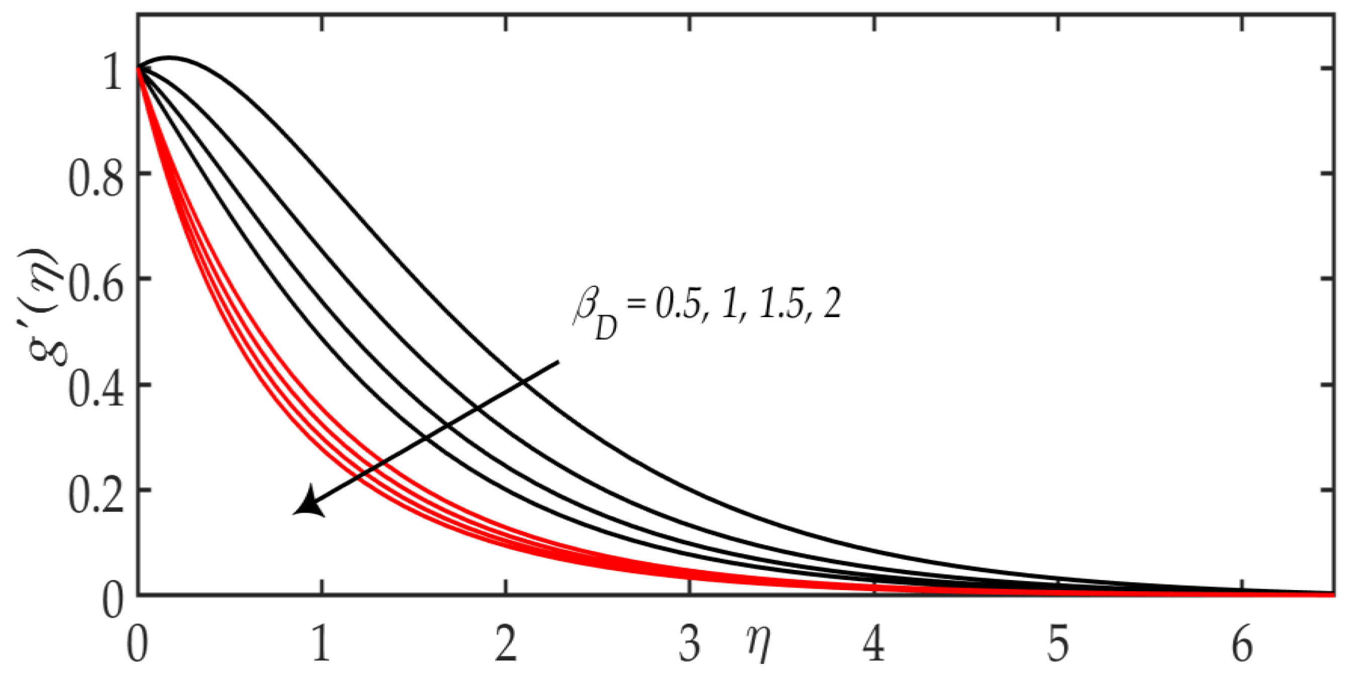
• It is observed that the permeability parameter and the magnetic field retard the velocity distribution while Richardson parameter boosts the velocity distribution.
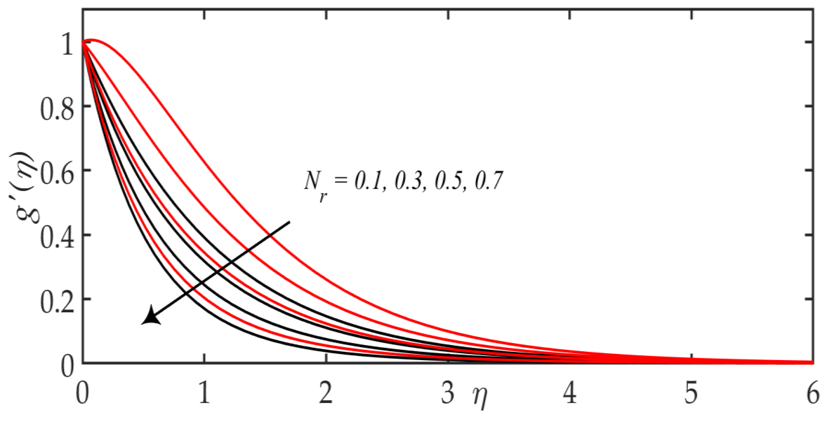
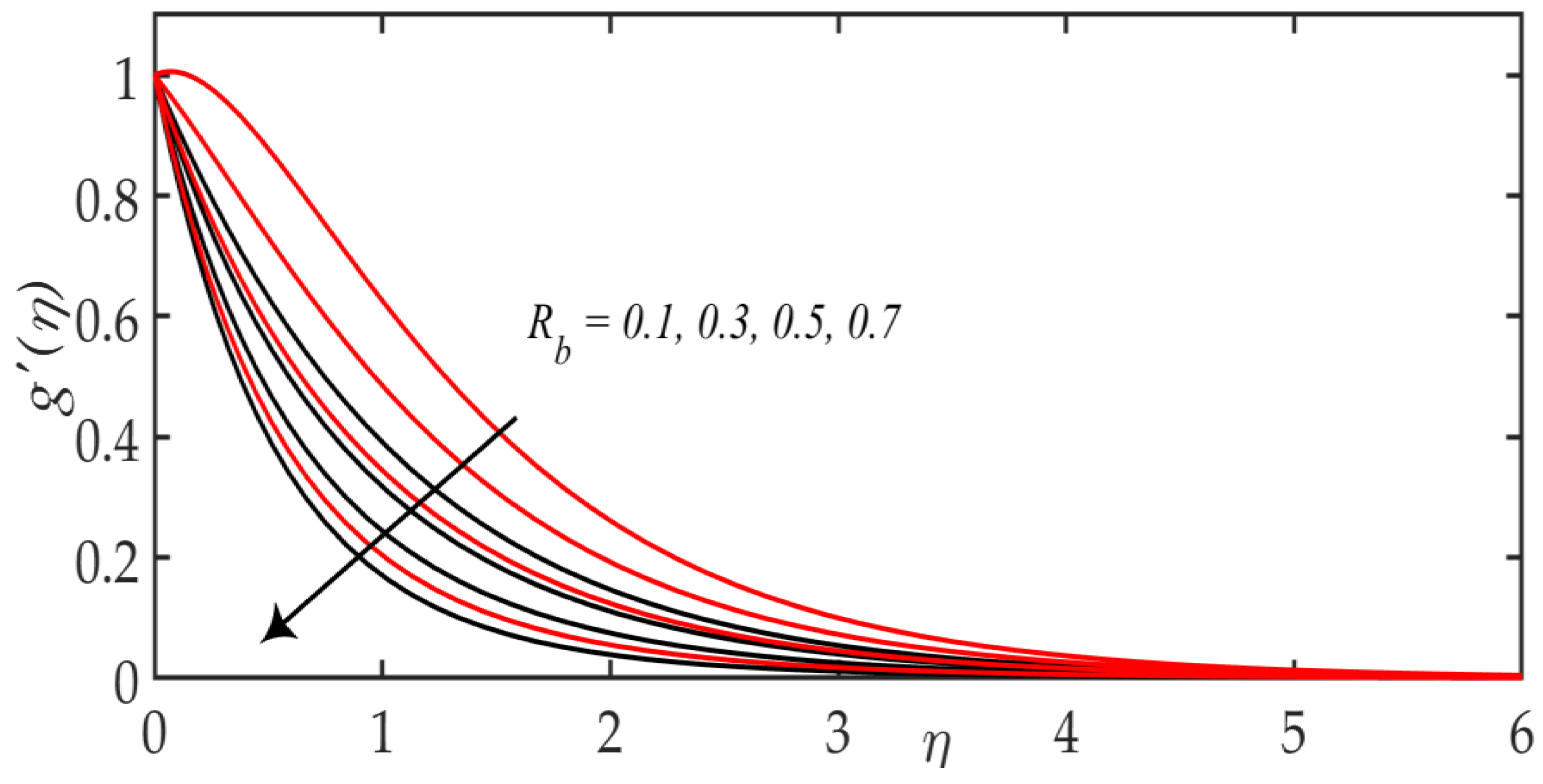
• Bioconvection Rayleigh number and Buoyancy proportion parametric quantity diminish the velocity distribution.
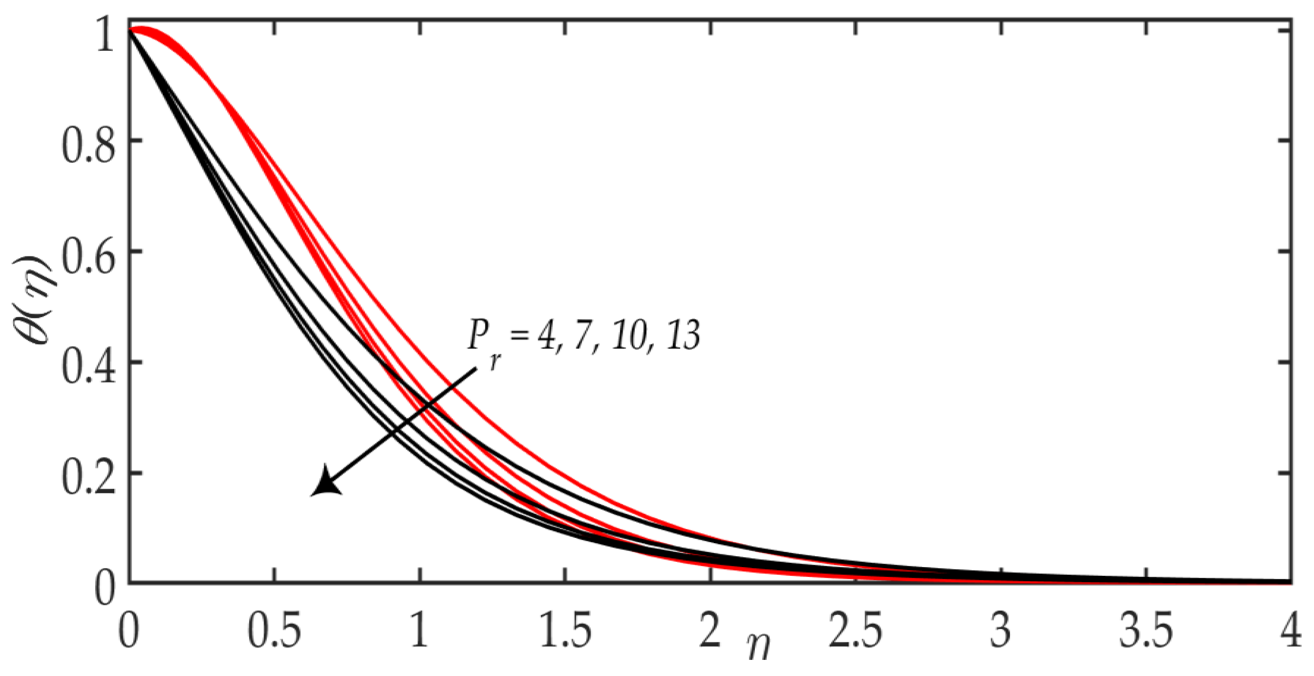
• Prandtl number elevates the temperature distribution while it has been demoted by enlarging the values of the magnetic field.
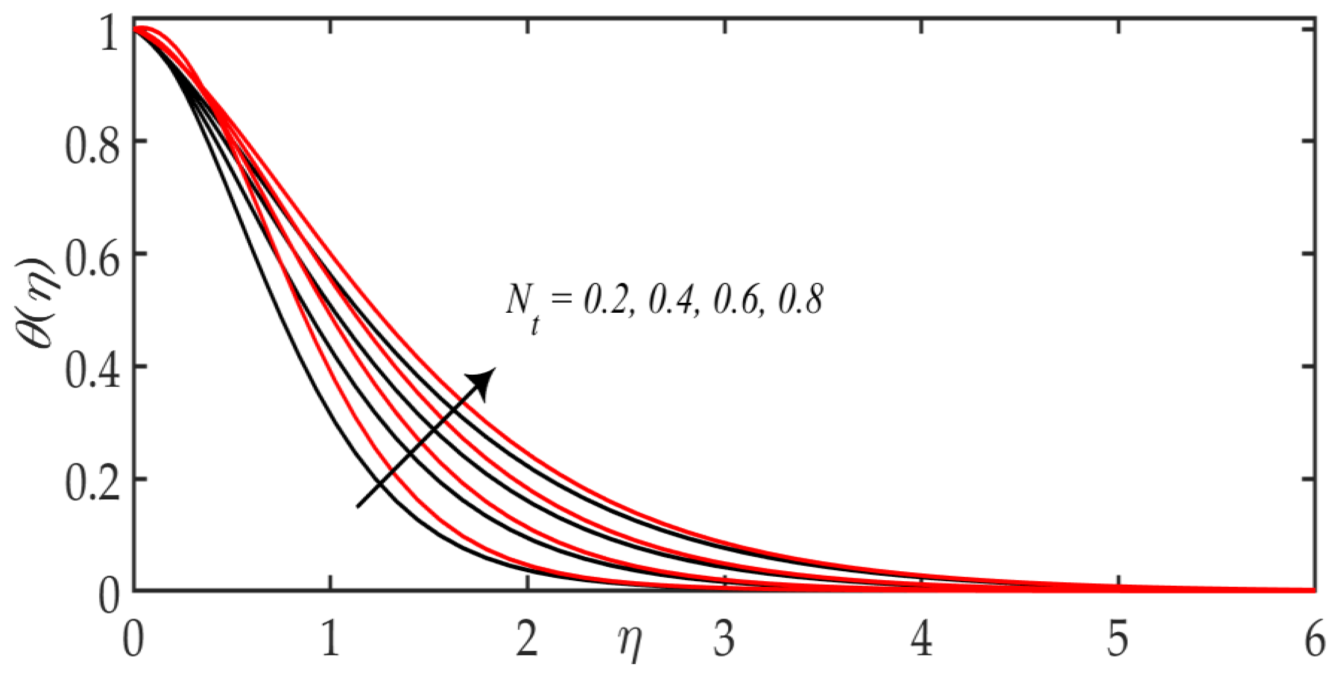
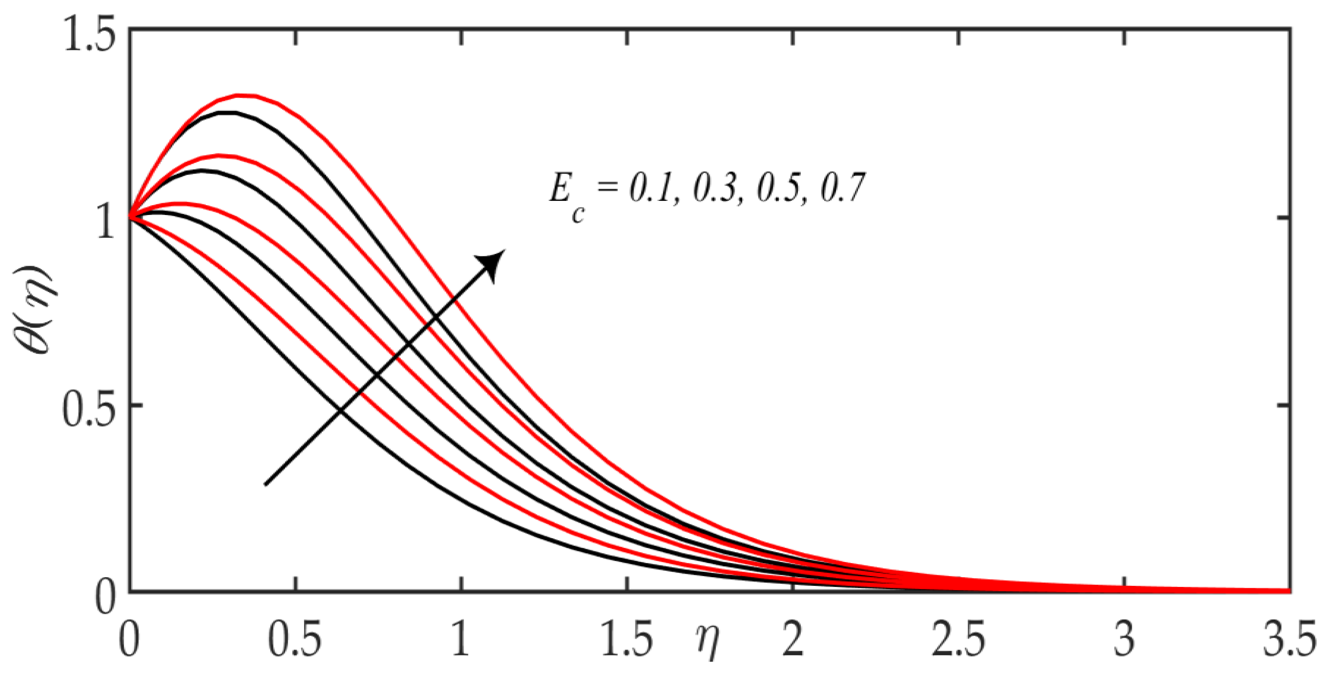
• The thermophoresis parameter and Eckert number significantly uplift the temperature distribution.
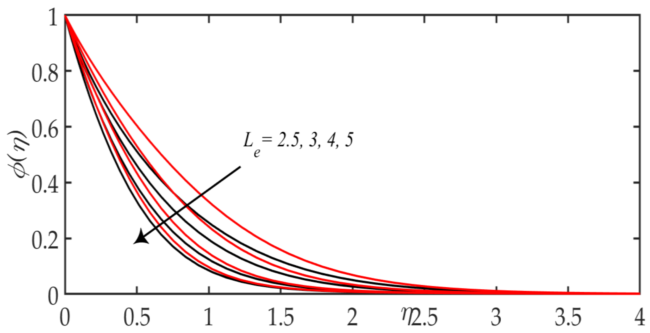
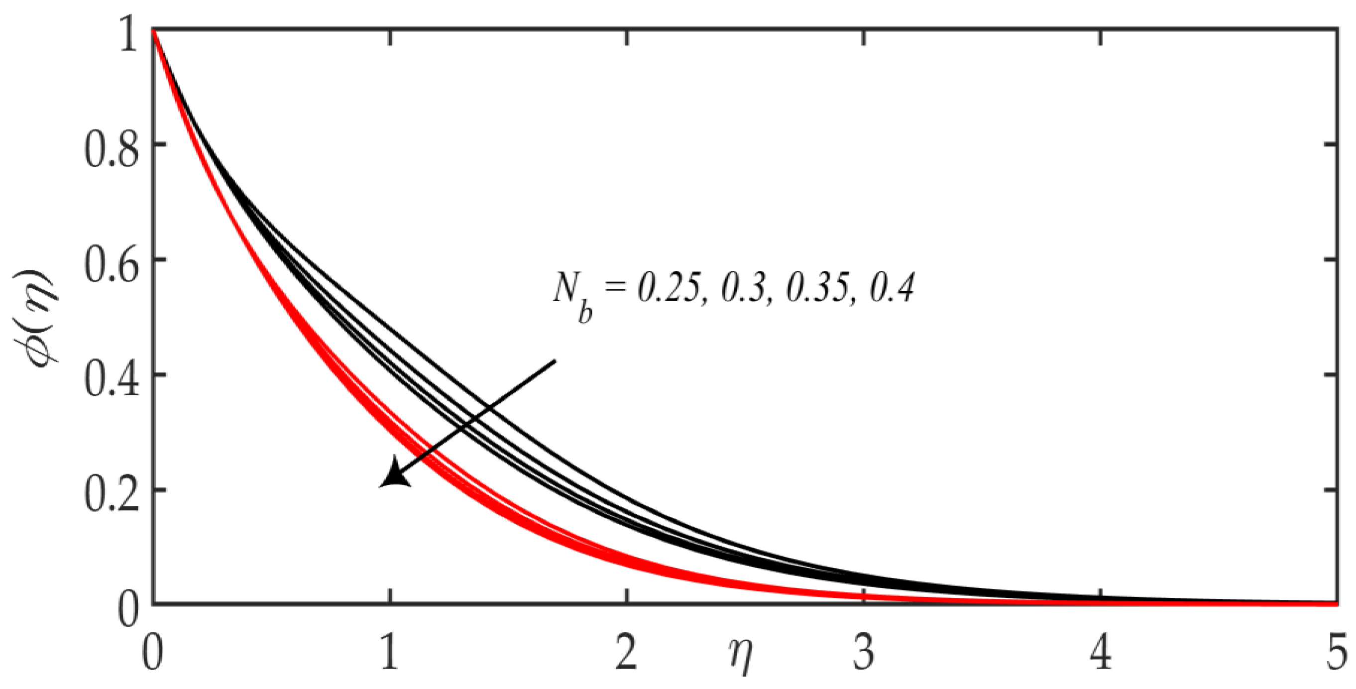
• Brownian-motion parameter and Lewis number suppress the concentration distribution, whereas an enhancement in the thermophoresis parameter actively elevates the concentration profile.
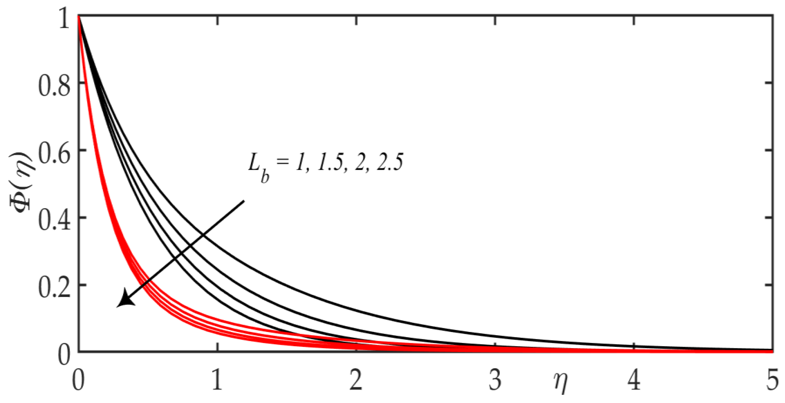
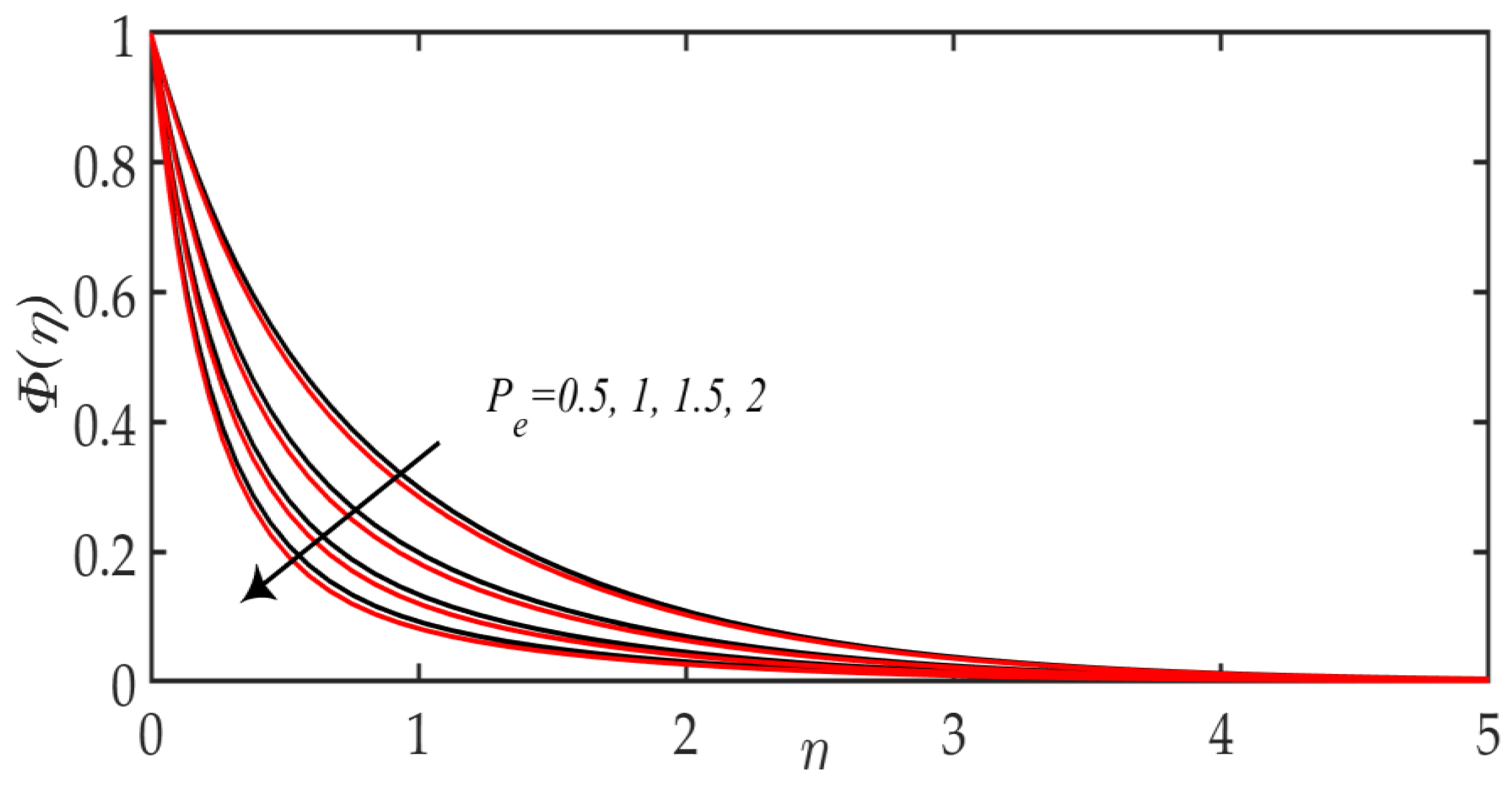
• Bioconvection Lewis number and Peclet number significantly demote the motile microorganism profile.
• The SLLM algorithm is smooth to establish and employ because the scheme based on a simple univariate linearization of nonlinear functions.
• The convergence speed of the SLLM technique can be willingly upgraded by applying successive over relaxation (SOR) method, the convergence was improved through relaxation parameter in the study.

References

1. Sakiadis, B.C. Boundary layer behavior on continuous solid surface, I: Boundary layer equations for two dimensional and axisymmetric flow. AIChE J. 1961, 26–28, 221–235. [Google Scholar] [CrossRef]
2. Crane, L.J. Flow past a stretching plane. Z. Angew. Math. Phys. 1970, 21, 645–647. [Google Scholar] [CrossRef]
3. Banks, W.H.H. Similarity solutions of the boundary layer equations for a stretching wall. J. de Mécanique Théorique et Appliquée 1983, 2, 92–375. [Google Scholar]
4. Gupta, P.S.; Gupta, A.S. Heat and mass transfer on a stretching sheet with suction or blowing. Can. J. Chem. Eng. 1977, 55, 744–746. [Google Scholar] [CrossRef]
5. Bujurke, N.M.; Biradar, S.N.; Hiremath, P.S. Second order fluid flow past a stretching sheet with heat transfer. Z. Angew. Math. Phys. 1987, 38, 890–892. [Google Scholar] [CrossRef]
6. Cortell, R. Viscous flow and heat transfer over a nonlinearly stretching sheet. Appl. Math. Comput. 2007, 184, 864–873. [Google Scholar] [CrossRef]
7. Shahzad, A.; Ali, R.; Khan, M. On the exact solution for axisymmetric flow and heat transfer over a nonlinear radially stretching sheet. Chin. Phys. Lett. 2012, 29, 084705. [Google Scholar] [CrossRef]
8. Hayat, T.; Shafiq, A.; Alsaedi, A.; Awais, M. MHD axisymmetric flow of third grade fluid between stretching sheets with heat transfer. Comput. Fluids 2013, 86, 103–108. [Google Scholar] [CrossRef]
9. Shateyi, S.; Makinde, O.D. Hydromagnetic stagnation-point flow towards a radially stretching convectively heated disk. Math. Prob. Eng. 2013, 2013, 616947. [Google Scholar] [CrossRef]
10. Khan, M.; Malik, R.; Munir, A. Mixed convective heat transfer to Sisko fluid over a radially stretching sheet in the presence of convective boundary conditions. AIP Adv. 2015, 5, 087178. [Google Scholar] [CrossRef] [Green Version]
11. Awais, M.; Hayat, T.; Irum, S.; Alsaedi, A. Heat Generation/Absorption Effects in a Boundary Layer Stretched Flow of Maxwell Nanofluid: Analytic and Numeric Solutions. PLoS ONE 2015, 10, e0129814. [Google Scholar] [CrossRef] [PubMed]
12. Ghalambaz, M.; Sheremet, M.A.; Pop, I. Free convection in a parallelogrammic porous cavity filled with a nanofluid using tiwari and das’ nanofluid model. PLoS ONE 2015, 10, e0126486. [Google Scholar] [CrossRef] [PubMed]
13. Choi, S.; Zhang, Z.; Yu, W.; Lockwood, F.; Grulke, E. Anomalous thermal conductivity enhancement in nanotube suspensions. Appl. Phys. Lett. 2001, 79, 2252–2254. [Google Scholar] [CrossRef]
14. Kuznetsov, A.V.; Nield, D.A. Natural convective boundary-layer flow of a nanofluid past a vertical plate. Int. J. Therm Sci. 2010, 49, 243–247. [Google Scholar] [CrossRef]
15. Noghrehabadadi, A.; Pourrajab, R.; Ghalambaz, M. Flow and heat transfer of nanofluids over stretching sheet taking into account partial slip and thermal convective boundary conditions. Heat Mass Transf. 2013, 49, 1357–1366. [Google Scholar] [CrossRef]
16. Zaraki, A.; Ghalambaz, M.; Chamkha, A.J.; Ghalambaz, M.; De Rossi, D. Theoretical analysis of natural convection boundary layer heat and mass transfer of nanofluids: Effects of size, shape and type of nanoparticles, type of base fluid and working temperature. Adv. Powder Technol. 2015, 26, 935–946. [Google Scholar] [CrossRef]
17. Ferdows, M.; Khan, M.S.; Alam, M.M.; Sun, S. MHD mixed convective boundary layer flow of a nanofluid through a porous medium due to an exponentially stretching sheet. Math. Probl. Eng. 2012, 2012, 408528. [Google Scholar] [CrossRef]
18. Bidin, B.; Nazar, R. Numerical solution of the boundary layer flow over an exponentially stretching sheet with thermal radiation. Eur. J. Sci. Res. 2009, 33, 710–717. [Google Scholar]
19. Shakhaoath Khan, M.D.; Mahmud Alamb, M.D.; Ferdows, M. Effects of magnetic field on radiative flow of a nanofluid past a stretching sheet. Procedia Eng. 2013, 56, 316–322. [Google Scholar] [CrossRef] [Green Version]
20. Mabood, F.; Khan, W.A.; Ismail, A.I.M. MHD boundary layer flow and heat transfer of nanofluids over a nonlinear stretching sheet: A numerical study. J. Magn. Magn. Mater. 2015, 374, 569–576. [Google Scholar] [CrossRef]
21. Freidoonimehr, N.; Rashidi, M.M.; Jalilpour, B. MHD stagnation-point flow past a stretching/shrinking sheet in the presence of heat generation/absorption and chemical reaction effects. J. Braz. Soc. Mech. Sci. Eng. 2016, 38, 1999–2008. [Google Scholar] [CrossRef]
22. Makinde, O.; Animasaun, I. Bioconvection in MHD nanofluid flow with nonlinear thermal radiation and quartic autocatalysis chemical reaction past an upper surface of a paraboloid of revolution. Int. J. Therm. Sci. 2016, 109, 159–171. [Google Scholar] [CrossRef]
23. Pour, M.S.; Nassab, S.G. Numerical investigation of forced laminar convection flow of nanofluids over a backward facing step under bleeding condition. J. Mech. 2012, 28, N7–N12. [Google Scholar] [CrossRef]
24. Abu-Nada, E. Numerical prediction of entropy generation in separated flows. Entropy 2005, 7, 234–252. [Google Scholar] [CrossRef] [Green Version]
25. Marin, M.; Vlase, S.; Ellahi, R.; Bhatti, M.M. On the partition of energies for backward in time problem of the thermoelastic materials with a dipolar structure. Symmetry 2019, 11, 863. [Google Scholar] [CrossRef] [Green Version]
26. Almutairi, F.; Khaled, S.M.; Ebaid, A. MHD flow of nanofluid with homogeneous-heterogeneous reactions in a porous medium under the influence of second-order velocity slip. Mathematics 2019, 7, 220. [Google Scholar] [CrossRef] [Green Version]
27. Khan, U.; Zaib, A.; Kahn, I.; Nasar, K.S.; Baleanu, D. Insights into the stability of mixed convective Darcy–Forchheimer flows of cross liquids from a vertical plate with consideration of the significant impact of velocity and thermal slip conditions. Mathematics 2020, 8, 31. [Google Scholar] [CrossRef] [Green Version]
28. Wan, N.A.; Maleki, A.; Nazari, M.A.; Tlili, I.; Shadloo, M.S. Thermal conductivity modeling of nanofluids contain MgO particles by employing different approaches. Symmetry 2020, 12, 206. [Google Scholar]
29. Jamalabadi, M.Y.A.; Ghasemi, M.; Alamian, R.; Wongwises, S.; Afrand, M.; Shadloo, M.S. Modeling of subcooled flow boiling with nanoparticles under the influence of a magnetic field. Symmetry 2019, 11, 1275. [Google Scholar] [CrossRef] [Green Version]
30. Safaei, M.R.; Ahmadi, G.; Goodarzi, M.S.; Shadloo, M.S.; Goshayeshi, H.R.; Dahari, M. Heat transfer and pressure drop in fully developed turbulent flows of graphene nanoplatelets–silver/water nanofluids. Fluids 2016, 1, 20. [Google Scholar] [CrossRef] [Green Version]
31. Shahrestani, M.I.; Maleki, A.; Shadloo, M.S.; Tlili, I. Numerical investigation of forced convective heat transfer and performance evaluation criterion of Al2O3/water nanofluid flow inside an axisymmetric microchannel. Symmetry 2020, 12, 120. [Google Scholar] [CrossRef] [Green Version]
32. Ellahi, R.; Hussain, F.; Abbas, S.A.; Sarafraz, M.M.; Goodarzi, M.; Shadloo, M.S. Study of two-phase newtonian nanofluid flow hybrid with hafnium particles under the effects of slip. Inventions 2020, 5, 6. [Google Scholar] [CrossRef] [Green Version]
33. Alamri, S.Z.; Ellahi, R.; Shehzad, N.; Zeeshan, A. Convective radiative plane poiseuille flow of nanofluid through porous medium with slip: An application of Stefan blowing. J. Mol. Liq. 2019, 273, 292–304. [Google Scholar] [CrossRef]
34. Alamri, S.Z.; Khan, A.A.; Azeez, M.; Ellahi, R. Effects of mass transfer on MHD second grade fluid towards stretching cylinder: A novel perspective of cattaneo–christov heat flux model. Phys. Lett. A 2019, 383, 276–281. [Google Scholar] [CrossRef]
35. Riaz, R.; Ellahi, R.; Bhatti, M.M.; Marin, M. Study of heat and mass transfer in the eyring-powell model of fluid propagating peristaltically through a rectangular complaint channel. Heat Transf. Res. 2019, 50, 1539–1560. [Google Scholar] [CrossRef]
36. Bhatti, M.M.; Ellahi, R.; Zeeshan, A.; Marin, M.; Ijaz, N. Numerical study of heat transfer and hall current impact on peristaltic propulsion of particle-fluid suspension with complaint wall properties. Mod. Phys. Lett. B 2019, 33, 1950439. [Google Scholar] [CrossRef]
37. Ellahi, R.; Sait, S.M.; Shehzad, N.; Ayaz, Z. A hybrid investigation on numerical and analytical solutions of electro-magnetohydrodynamics flow of nanofluid through porous media with entropy generation. Int. J. Numer. Methods Heat Fluid Flow 2020, 30, 834–854. [Google Scholar] [CrossRef]
38. Sarafraz, M.M.; Pourmehran, O.; Yang, B.; Arjomandi, M.; Ellahi, R. Pool boiling heat transfer characteristics of iron oxide nano-suspension under constant magnetic field. Int. J. Therm. Sci. 2020, 147, 106131. [Google Scholar] [CrossRef]
39. Platt, J.R. “Bioconvection patterns” in cultures of free-swimming organisms. Science 1961, 133, 1766–1767. [Google Scholar] [CrossRef]
40. Ghorai, S.; Hill, N.A. Wavelengths of gyrotactic plumes in bioconvection. Bull. Math. Biol. 2000, 62, 429–450. [Google Scholar] [CrossRef]
41. Kuznetsov, A.V.; Avramenko, A.A. Effect of small particles on the stability of bioconvection in a suspension of gyrotactic microorganisms in a layer of finite depth. Int. Commun. Heat Mass Transf. 2004, 31, 1–10. [Google Scholar] [CrossRef]
42. Khan, W.A.; Makinde, O.D. MHD nanofluid bioconvection due to gyrotactic microorganisms over a convectively heat stretching sheet. Int. J. Therm. Sci. 2014, 81, 118–124. [Google Scholar] [CrossRef]
43. Raees, A.; Hang, X.U.; Qiang, S.U.N.; Pop, I. Mixed convection in gravity-driven nano-liquid film containing both nanoparticles and gyrotactic microorganisms. Appl. Math. Mech. 2015, 36, 163–178. [Google Scholar] [CrossRef]
44. Kuznetsov, A.V.; Nield, D.A. Double-diffusive natural convective boundary layer flow of a nanofluid past a vertical surface. Int. J. Therm. Sci. 2011, 50, 712–717. [Google Scholar] [CrossRef]
45. Sivaraj, R.; Animasaun, I.L.; Olabiyi, A.S.; Saleem, S.; Sandeep, N. Gyrotactic microorganisms and thermoelectric effects on the dynamics of 29 nm CuO-water nanofluid over an upper horizontal surface of paraboloid of revolution. Multidiscip. Model. Mater. Struct. 2018, 14, 695–721. [Google Scholar] [CrossRef]
46. Amirsom, N.A.; Uddin, M.; Basir, M.; Faisal, M.; Kadir, A.; Bég, O.A.; Ismail, M.; Izani, A. Computation of melting dissipative magnetohydrodynamic nanofluid bioconvection with second-order slip and variable thermophysical properties. Appl. Sci. 2019, 9, 2493. [Google Scholar] [CrossRef] [Green Version]
47. Waqas, H.; Khan, S.U.; Imran, M.; Bhatti, M.M. Thermally developed falkner–skan bioconvection flow of a magnetized nanofluid in the presence of a motile gyrotactic microorganism: Buongiorno’s nanofluid model. Phys. Scr. 2019, 94, 115304. [Google Scholar] [CrossRef]
48. Waqas, H.; Khan, S.U.; Hassan, M.; Bhatti, M.M.; Imran, M. Analysis on the bioconvection flow of modified second-grade nanofluid containing gyrotactic microorganisms and nanoparticles. J. Mol. Liq. 2019, 291, 111231. [Google Scholar] [CrossRef]
49. Ferdows, M.; Reddy, M.G.; Alzahrani, F.; Sun, S. Heat and mass transfer in a viscous nanofluid containing a gyrotactic micro-organism over a stretching cylinder. Symmetry 2019, 11, 1131. [Google Scholar] [CrossRef] [Green Version]
50. Khan, W.A.; Rashad, A.M.; Abdou, M.M.M.; Tlili, I. Natural bioconvection flow of a nanofluid containing gyrotactic microorganisms about a truncated cone. Eur. J. Mech. B Fluids 2019, 75, 133–142. [Google Scholar] [CrossRef]
51. Ferdows, M.; Reddy, M.G.; Sun, S.; Alzahrani, F. Two-dimensional gyrotactic microorganisms flow of hydromagnetic power law nanofluid past an elongated sheet. Adv. Mech. Eng. 2019, 11. [Google Scholar] [CrossRef]
52. Trefethen, L.N. Spectral Methods in MATLAB; SIAM: Philadelphia, PA, USA, 2000; Volume 10. [Google Scholar]
53. Akbar, N.S.; Khan, Z.H. Magnetic field analysis in a suspension of gyrotactic microorganisms and nanoparticles over a stretching surface. J. Magn. Magn. Mater. 2016, 410, 72–80. [Google Scholar] [CrossRef]
54. Khan, W.A.; Pop, I. Boundary-layer flow of a nanofluid past a stretching sheet. Int. J. Heat Mass Transf. 2010, 53, 2477–2483. [Google Scholar] [CrossRef]
55. Wang, C.Y. Free convection on a vertical stretching surface. J. Appl. Math. Mech. 1989, 69, 418–420. [Google Scholar] [CrossRef]
Figure 1. Flow structure through a stretch elastic plate.
Mathematics 08 00380 g001
Figure 2. Variation of β D and M on velocity distribution. Black line: M   =   0 , Red line: M   =   3 .
Mathematics 08 00380 g002
Figure 3. Variation of N r and G r R e 2 on velocity distribution. Black line: G r R e 2   =   5.5 , Red line: G r R e 2   =   10.5 .
Mathematics 08 00380 g003
Figure 4. Variation of R b and G r R e 2 on velocity distribution. Black line: G r R e 2   =   5.5 , Red line: G r R e 2     = 10.5 .
Mathematics 08 00380 g004
Figure 5. Variation of P r and M on temperature profile. Black line: M   =   0 , Red line: M   =   3 .
Mathematics 08 00380 g005
Figure 6. Variation of N b and N t on temperature profile. Black line: N b   =   0.2 , Red line: N b   =   0.5 .
Mathematics 08 00380 g006
Figure 7. Variation of N b and E c on temperature profile. Black line: N b   =   0.2 , Red line: N b   =   0.5 .
Mathematics 08 00380 g007
Figure 8. Variation of N t and L e on concentration profile. Solid line: N t   =   5 , Dotted line: N t   =   10 .
Mathematics 08 00380 g008
Figure 9. Variation of N b and L e on concentration profile. Solid line: L e   =   1.5 , Dotted line: L e   =   2.0 .
Mathematics 08 00380 g009
Figure 10. Variation of P e and L b on microorganism profile. Solid line: P e   =   0.5 , Dotted line: P e   =   2.0 .
Mathematics 08 00380 g010
Figure 11. Variation of P e and Ω d on microorganism profile. Solid line: Ω d   =   0.1 , Dotted line: Ω d   =   0.3 .
Mathematics 08 00380 g011