A Numerical Computation of Zeros of q-Generalized Tangent-Appell Polynomials

Abstract

The intended objective of this study is to define and investigate a new class of q-generalized tangent-based Appell polynomials by combining the families of 2-variable q-generalized tangent polynomials and q-Appell polynomials. The investigation includes derivations of generating functions, series definitions, and several important properties and identities of the hybrid q-special polynomials. Further, the analogous study for the members of this q-hybrid family are illustrated. The graphical representation of its members is shown, and the distributions of zeros are displayed.

1. Introduction and Preliminaries

The area of q-calculus in the last three decades act as a bridge between engineering sciences and mathematics. Recently, research in the area of q-calculus has shown worthy of attention due to its applicative diversification in various fields such as mathematics, physics, and engineering. The q-analogues of many orthogonal polynomials and functions expect a pleasant structure, and help one to remember their classical counterpart. The q-standard notations and definitions reviewed here are taken from [1].

The q-analogue of a number $a\in \mathbb{C}$ and factorial function are specified as

$${\left[a\right]}_q=\frac{1-q^a}{1-q},q\in \mathbb{C}\backslash \left\{1\right\},$$

(1)

$${\left[n\right]}_q!=\prod _{m=1}^n{\left[m\right]}_q={\left[1\right]}_q{\left[2\right]}_q{\left[3\right]}_q\cdots {\left[n\right]}_q,{\left[0\right]}_q!=1,n\in \mathbb{N},0<q<1.$$

(2)

The q-binomial coefficient ${\left[\genfrac{}{}{0pt}{}{n}{k}\right]}_q$ is specified as

$${\left[\genfrac{}{}{0pt}{}{n}{k}\right]}_q=\frac{{\left[n\right]}_q!}{{\left[k\right]}_q!{[n-k]}_q!},k=0,1,2,\cdots ,n,n\in {\mathbb{N}}_0.$$

(3)

The q-power basis is specified as

$${(u+v)}_q^n=\sum _{k=0}^n{\left[\genfrac{}{}{0pt}{}{n}{k}\right]}_q{q}^{k(k-1)/2}{u}^{n-k}{v}^k,n\in {\mathbb{N}}_0.$$

(4)

The q-exponential functions are specified by

$$e_q\left(u\right)=\sum _{k=0}^{\infty }\frac{u^k}{{\left[k\right]}_q!}{,0<\left|q\right|<1,\left|u\right|<|1-q|}^{-1},$$

(5)

$$E_q\left(u\right)=\sum _{k=0}^{\infty }{q}^{k(k-1)/2}\frac{u^k}{{\left[k\right]}_q!},0<\left|q\right|<1,u\in \mathbb{C}$$

(6)

and satisfy the following relation

$$e_q\left(t\right)E_q(-t)=E_q\left(t\right)e_q(-t)=1.$$

(7)

The q-derivative $D_q$ of functions $e_q\left(u\right)$ and $E_q\left(u\right)$ are given by

$$D_q{e}_q\left(ut\right)=t{e}_q\left(ut\right),D_q{E}_q\left(ut\right)=t{E}_q\left(qut\right).$$

(8)

The q-derivative operator $D_q$ for any two arbitrary functions $f\left(u\right)$ and $g\left(u\right)$ satisfies the following product and quotient relations:

$$D_q\left(f\left(u\right)g\left(u\right)\right)=f\left(qu\right)D_{q}g\left(u\right)+g\left(u\right)D_{q}f\left(u\right)=f\left(u\right)D_{q}g\left(u\right)+g\left(qu\right)D_{q}f\left(u\right),$$

(9)

$$D_q\left(\frac{f\left(u\right)}{g\left(u\right)}\right)=\frac{g\left(qu\right)D_{q}f\left(u\right)-f\left(qu\right)D_{q}g\left(u\right)}{g\left(u\right)g\left(qu\right)}=\frac{g\left(u\right)D_{q}f\left(u\right)-f\left(u\right)D_{q}g\left(u\right)}{g\left(u\right)g\left(qu\right)}.$$

(10)

The tangent numbers and polynomials and their q-analogue have enormous applications in analytic number theory, physics, and other related areas. Various properties of these polynomials are studied and investigated by many mathematicians, see, for example, [2,3,4]. Very recently, Yasmin et al. [5] introduced the 2-variable q-generalized tangent polynomials $C_{n,m,q}\left(u\right)$ and established certain interesting results for them. We recall the following definition.

Definition 1.

The 2-variable q-generalized tangent polynomials (qGTP) $C_{n,m,q}\left(u\right)$ is defined as [5]:

$$\left(\frac{2}{e_q\left(mt\right)+1}\right)e_q\left(ut\right)E_q\left(vt\right)=\sum _{n=0}^{\infty }{C}_{n,m,q}(u,v)\frac{t^n}{{\left[n\right]}_q!},\left(\left|mt\right|<\pi ,m\in {\mathbb{R}}^{+}\right).$$

(11)

We have

$\underset{m\to 1}{lim}{C}_{n,m,q}(u,v)={\epsilon }_{n,q}(u,v)$, (2-variable q-Euler polynomials (qEP) [6])

$\underset{m\to 2}{lim}{C}_{n,m,q}(u,v)=T_{n,q}(u,v)$, (2-variable q-tangent polynomials (qTP) [7])

$C_{n,m,q}(0,0):=C_{n,m,q}$ (q-generalized tangent numbers (qGTN) [5])

The series representation of qGTP $C_{n,m,q}(u,v)$ is given by

$$C_{n,m,q}(u,v)=\sum _{r=0}^n\sum _{k=0}^r{\left[\genfrac{}{}{0pt}{}{n}{r}\right]}_q{\left[\genfrac{}{}{0pt}{}{r}{k}\right]}_q{C}_{n-r,m,q}{q}^{k(k-1)/2}{u}^{r-k}{v}^k.$$

(12)

A vital class of polynomial sequences known as the Appell polynomials is introduced by Appell [8]. Later, the class of q-Appell polynomials ${\left\{A_{n,q}\left(u\right)\right\}}_{n=0}^{\infty }$ was introduced by Al-Salam [9] and studied some of its properties. These polynomials arise in chemistry, theoretical physics, and different branches of mathematics such as numerical analysis, number theory, and in the study of polynomial expansion of analytic function.

Definition 2.

The q-Appell polynomials $A_{n,q}\left(u\right)$ are defined by the following generating function [9]:

$$A_q\left(t\right)e_q\left(ut\right)=\sum _{n=0}^{\infty }{A}_{n,q}\left(u\right)\frac{t^n}{{\left[n\right]}_q!},0<q<1,$$

(13)

where

$$A_q\left(t\right):=\sum _{n=0}^{\infty }{A}_{n,q}\frac{t^n}{{\left[n\right]}_q!},A_{0,q}=1;A_q\left(t\right)\ne 0$$

(14)

is an analytic function at $t=0$ and $A_{n,q}:=A_{n,q}\left(0\right)$ are q-Appell numbers.

The series representation of q-Appell polynomials is given by

$$A_{n,q}\left(u\right)=\sum _{k=0}^n{\left[\genfrac{}{}{0pt}{}{n}{k}\right]}_q{A}_{k,q}{u}^{n-k}.$$

(15)

A significant part of the investigation of any polynomials is to discover its determinant definition. Recently, Keleshteri et al. [10] gave the determinant definition of the q-Appell polynomials, according to which the q-Appell polynomials $A_{n,q}\left(u\right)$ of degree n can be expressed in the following determinant form:

$$A_{0,q}\left(u\right)=\frac{1}{{\beta }_{0,q}},$$

$$A_{n,q}\left(u\right)=\frac{{(-1)}^n}{{\left({\beta }_{0,q}\right)}^{n+1}}\left|\begin{array}{cccccc}1& u& u^2& \cdots & u^{n-1}& u^n\\ {\beta }_{0,q}& {\beta }_{1,q}& {\beta }_{2,q}& \cdots & {\beta }_{n-1,q}& {\beta }_{n.q}\\ 0& {\beta }_{0,q}& {\left[\genfrac{}{}{0pt}{}{2}{1}\right]}_q{\beta }_{1,q}& \cdots & {\left[\genfrac{}{}{0pt}{}{n-1}{1}\right]}_q{\beta }_{n-2,q}& {\left[\genfrac{}{}{0pt}{}{n}{1}\right]}_q{\beta }_{n-1,q}\\ 0& 0& {\beta }_0& \cdots & {\left[\genfrac{}{}{0pt}{}{n-1}{2}\right]}_q{\beta }_{n-3,q}& {\left[\genfrac{}{}{0pt}{}{n}{2}\right]}_q{\beta }_{n-2,q}\\ .& .& .& \cdots & .& .\\ .& .& .& \cdots & .& .\\ 0& 0& 0& \cdots & {\beta }_{0,q}& {\left[\genfrac{}{}{0pt}{}{n}{n-1}\right]}_q{\beta }_{1,q}\end{array}\right|,$$

(16)

where $n=1,2,3,\cdots$; ${\beta }_{0,q}\ne 0$ and

$${\beta }_{0,q}=\frac{1}{A_{0,q}},$$

$${\beta }_{n,q}=-\frac{1}{A_{0,q}}\left(\sum _{k=1}^n{\left[\genfrac{}{}{0pt}{}{n}{k}\right]}_q{A}_{k,q}{\beta }_{n-k,q}\right),n=1,2,3,\cdots .$$

(17)

Various members of the q-Appell family can be obtained by choosing a suitable function $A_q\left(t\right)$ in the generating function expressed in Equation (13). Some of its members along with their name, generating function, and series definition, are mentioned in

Table 1. Certainmembers belonging to the q-Appell family.

		Name of q-Special
S. No.	${\mathit{A}}_{\mathit{q}}\left(\mathit{t}\right)$	Polynomials and Its	Generating Function	Series Definition
		Associated Numbers
I	$\frac{t}{e_q\left(t\right)-1}$	q-Bernoulli polynomials;	$\frac{t}{e_q\left(t\right)-1}{e}_q\left(ut\right)={\sum }_{n=0}^{\infty }{B}_{n,q}\left(u\right)\frac{t^n}{{\left[n\right]}_q!}$	$B_{n,q}\left(u\right)={\sum }_{k=0}^n{\left[\genfrac{}{}{0pt}{}{n}{k}\right]}_q{B}_{k,q}{u}^{n-k}$
		q-Bernoulli numbers	$\frac{t}{e_q\left(t\right)-1}={\sum }_{n=0}^{\infty }{B}_{n,q}\frac{t^n}{{\left[n\right]}_q!}$
		[11,12]	$B_{n,q}:=B_{n,q}\left(0\right)$
II	$\frac{2}{e_q\left(t\right)+1}$	q-Euler polynomials;	$\frac{2}{e_q\left(t\right)+1}{e}_q\left(ut\right)={\sum }_{n=0}^{\infty }{\epsilon }_{n,q}\left(u\right)\frac{t^n}{{\left[n\right]}_q!}$	${\epsilon }_{n,q}\left(u\right)={\sum }_{k=0}^n{\left[\genfrac{}{}{0pt}{}{n}{k}\right]}_q{\epsilon }_{k,q}{u}^{n-k}$
		q-Euler numbers	$\frac{2}{e_q\left(t\right)+1}={\sum }_{n=0}^{\infty }{\epsilon }_{n,q}\frac{t^n}{{\left[n\right]}_q!}$
		[6,12]	${\epsilon }_{n,q}:={\epsilon }_{n,q}\left(0\right)$

.

The hybrid type q-special polynomials are a subject of recent interest. In the present work, we introduce and investigate the properties of q-generalized tangent-based Appell polynomials. Their series expansion, determinant form, summation formulae, and differential recurrence relations are obtained in Section 2. In Section 3, some identities and relations involving q-generalized tangent-based Appell numbers and polynomials are derived. In the last section, the graphical representation of its members are shown for different values of indices using Matlab. Further, the distributions of zeros of these members are displayed.

2. q-Generalized Tangent-Appell Polynomials

In this section, we introduce the q-generalized tangent-based Appell polynomials (qGTAP) by means of a generating function. Further, some properties of these polynomials are also obtained.

Using the expansion expressed in Equation (5) in the generating function expressed in Equation (13) of q-Appell polynomials and then replacing powers of u ie $u^0,u^1,u^2,\cdots ,u^n$ by the corresponding qGTP $C_{0,m,q}(u,v),C_{1,m,q}(u,v),$$C_{2,m,q}(u,v),\cdots ,C_{n,m,q}(u,v)$ and thereafter using the generating function expressed in Equation (11) of qGTP $C_{n,m,q}(u,v)$ and denoting the resultant q-generalized tangent-based Appell polynomials by ${}_{C}A_{n,q}^{\left(m\right)}(u,v)$, the following definition is obtained:

Definition 3.

The q-generalized tangent-Appell polynomials (qGTAP) ${}_{C}A_{n,q}^{\left(m\right)}(u,v)$$(q\in \mathbb{C},0<|q|<1,$$\left|mt\right|<\pi ,m\in {\mathbb{R}}^{+})$ are defined by means of the following generating function:

$$\left(\frac{2}{e_q\left(mt\right)+1}\right)A_q\left(t\right)e_q\left(ut\right)E_q\left(vt\right)=\sum _{n=0}^{\infty }{}_{C}A_{n,q}^{\left(m\right)}(u,v)\frac{t^n}{{\left[n\right]}_q!}.$$

(18)

When $u=v=0$, ${}_{C}A_{n,q}^{\left(m\right)}(0,0):={}_{C}A_{n,q}^{\left(m\right)}$ are the corresponding q-generalized tangent-Appell numbers and are defined as

$$\left(\frac{2}{e_q\left(mt\right)+1}\right)A_q\left(t\right)=\sum _{n=0}^{\infty }{}_{C}A_{n,q}^{\left(m\right)}\frac{t^n}{{\left[n\right]}_q!}.$$

(19)

Selecting suitable function $A_q\left(t\right)$ and appropriate values of m in the generating function expressed in Equation (18), several members belonging to the family of qGTAP ${}_{C}A_{n,q}^{\left(m\right)}(u,v)$ are obtained. These members are listed in

Table 2. Certain members belonging to the qGTAP ${}_{C}A_{n,q}^{\left(m\right)}(u,v)$.

S. No.	${\mathit{A}}_{\mathit{q}}\left(\mathit{t}\right)$	Name of the	Generating Function	Generating Function
		Resultant Member	of Resultant Polynomial	of Resultant Number
I	$A_q\left(t\right)=\frac{t}{e_q\left(t\right)-1}$	q-generalized tangent	$\left(\frac{2}{e_q\left(mt\right)+1}\right)\left(\frac{t}{e_q\left(t\right)-1}\right)e_q\left(ut\right)E_q\left(vt\right)$	$\left(\frac{2}{e_q\left(mt\right)+1}\right)\left(\frac{t}{e_q\left(t\right)-1}\right)$
		-Bernoulli polynomials (qGTBP)	$={\sum }_{n=0}^{\infty }{}_{C}B_{n,q}^{\left(m\right)}(u,v)\frac{t^n}{{\left[n\right]}_q!}$	$={\sum }_{n=0}^{\infty }{}_{C}B_{n,q}^{\left(m\right)}\frac{t^n}{{\left[n\right]}_q!}$
II	$A_q\left(t\right)=\frac{2}{e_q\left(t\right)+1}$	q-generalized tangent	$\left(\frac{2}{e_q\left(mt\right)+1}\right)\left(\frac{2}{e_q\left(t\right)+1}\right)e_q\left(ut\right)E_q\left(vt\right)$	$\left(\frac{2}{e_q\left(mt\right)+1}\right)\left(\frac{2}{e_q\left(t\right)+1}\right)$
		-Euler polynomials (qGTEP)	$={\sum }_{n=0}^{\infty }{}_C\epsilon _{n,q}^{\left(m\right)}(u,v)\frac{t^n}{{\left[n\right]}_q!}$	$={\sum }_{n=0}^{\infty }{}_C\epsilon _{n,q}^{\left(m\right)}\frac{t^n}{{\left[n\right]}_q!}$

.

Remark 1.

As for $m=2$, the qGTP $C_{n,m,q}\left(u\right)$ reduces to the qTP $T_{n,q}(u,v)$. Thus, for the same choice of m, the results of qGTBP ${}_{C}B_{n,q}^{\left(m\right)}(u,v)$ and qGTEP ${}_C\epsilon _{n,q}^{\left(m\right)}(u,v)$ (Table 2) reduces to the corresponding results of the q-tangent Bernoulli and q-tangent Euler polynomials.

Remark 2.

As for $m=1$, the qGTP $C_{n,m,q}\left(u\right)$ reduces to the qEP ${\epsilon }_{n,q}^{\left(m\right)}(u,v)$. Thus, for the same choice of m, the results of qGTBP ${}_{C}B_{n,q}^{\left(m\right)}(u,v)$ and qGTEP ${}_C\epsilon _{n,q}^{\left(m\right)}(u,v)$ (Table 2) reduces to the corresponding results of the q-Euler Bernoulli and 2-iterated q-Euler polynomials.

The determinant definitions are helpful in finding solutions to general linear interpolation problems and can likewise be valuable for calculation purposes. The recent establishment of determinant definitions for various hybrid polynomials (see, for instance, [10,13]) offers inspiration to establish the determinant definition for qGTAP ${}_{C}A_{n,q}^{\left(m\right)}(u,v)$ is characterized as follows:

Definition 4.

The following determinant form for the qGTAP ${}_{C}A_{n,q}^{\left(m\right)}(u,v)$ of degree n holds true:

$${}_{C}A_{n,q}^{\left(m\right)}(u,v)=\frac{1}{{\beta }_{0,q}},$$

$${}_{C}A_{n,q}^{\left(m\right)}(u,v)=\frac{{(-1)}^n}{{\left({\beta }_{0,q}\right)}^{n+1}}\left|\begin{array}{cccccc}1& C_{1,m,q}(u,v)& C_{2,m,q}(u,v)& \cdots & C_{n-1,m,q}(u,v)& C_{n,m,q}(u,v)\\ {\beta }_{0,q}& {\beta }_{1,q}& {\beta }_{2,q}& \cdots & {\beta }_{n-1,q}& {\beta }_{n,q}\\ 0& {\beta }_{0,q}& {\left[\genfrac{}{}{0pt}{}{2}{1}\right]}_q{\beta }_{1,q}& \cdots & {\left[\genfrac{}{}{0pt}{}{n-1}{1}\right]}_q{\beta }_{n-2,q}& {\left[\genfrac{}{}{0pt}{}{n}{1}\right]}_q{\beta }_{n-1,q}\\ 0& 0& {\beta }_{0,q}& \cdots & {\left[\genfrac{}{}{0pt}{}{n-1}{2}\right]}_q{\beta }_{n-3,q}& {\left[\genfrac{}{}{0pt}{}{n}{2}\right]}_q{\beta }_{n-2,q}\\ .& .& .& \cdots & .& .\\ .& .& .& \cdots & .& .\\ 0& 0& 0& \cdots & {\beta }_{0,q}& {\left[\genfrac{}{}{0pt}{}{n}{n-1}\right]}_q{\beta }_{1,q}\end{array}\right|,$$

(20)

where $n=1,2,3,\cdots$; ${\beta }_{0,q}\ne 0$ and

$${\beta }_{0,q}=\frac{1}{{}_{C}A_{0,q}^{\left(m\right)}},$$

$${\beta }_{n,q}=-\frac{1}{{}_{C}A_{0,q}^{\left(m\right)}}\left(\sum _{k=1}^n{\left[\genfrac{}{}{0pt}{}{n}{k}\right]}_q{}_{C}A_{n,q}^{\left(m\right)}{\beta }_{n-k,q}\right),n=1,2,3,\cdots .$$

(21)

Remark 3.

The qGTBP ${}_{C}B_{n,q}^{\left(m\right)}(u,v)$ and qGTEP ${}_C\epsilon _{n,q}^{\left(m\right)}(u,v)$ mentioned in Table 2 are particular members of qGTAP ${}_{C}A_{n,q}^{\left(m\right)}(u,v)$. Thus, by making appropriate choices for the coefficients ${\beta }_{0,q}$ and ${\beta }_{k,q}$$(k=1,2,\cdots ,n)$ in the determinant definition of qGTAP ${}_{C}A_{n,q}^{\left(m\right)}(u,v)$, the determinant definitions of qGTBP ${}_{C}B_{n,q}^{\left(m\right)}(u,v)$ and qGTEP ${}_C\epsilon _{n,q}^{\left(m\right)}(u,v)$ can be obtained.

For instance, taking ${\beta }_{0,q}=1$ and ${\beta }_{k,q}=\frac{1}{{[k+1]}_q}$ $(k=1,2,\cdots ,n)$ in Equation (20), the following determinant form of qGTBP ${}_{C}B_{n,q}^{\left(m\right)}(u,v)$ is obtained:

Definition 5.

The following determinant form for the qGTBP ${}_{C}B_{n,q}^{\left(m\right)}(u,v)$ of degree n holds true:

$${}_{C}B_{0,q}^{\left(m\right)}(u,v)=1,$$

$$\begin{array}{c}{}_{C}B_{n,q}^{\left(m\right)}(u,v)={(-1)}^n\left|\begin{array}{cccccc}1& C_{1,m,q}(u,v)& C_{2,m,q}(u,v)& \cdots & C_{n-1,m,q}(u,v)& C_{n,m,q}(u,v)\\ 1& \frac{1}{{\left[2\right]}_q}& \frac{1}{{\left[3\right]}_q}& \cdots & \frac{1}{{\left[n\right]}_q}& \frac{1}{{[n+1]}_q}\\ 0& 1& {\left[\genfrac{}{}{0pt}{}{2}{1}\right]}_q\frac{1}{{\left[2\right]}_q}& \cdots & {\left[\genfrac{}{}{0pt}{}{n-1}{1}\right]}_q\frac{1}{{[n-1]}_q}& {\left[\genfrac{}{}{0pt}{}{n}{1}\right]}_q\frac{1}{{\left[n\right]}_q}\\ 0& 0& 1& \cdots & {\left[\genfrac{}{}{0pt}{}{n-1}{2}\right]}_q\frac{1}{{[n-2]}_q}& {\left[\genfrac{}{}{0pt}{}{n}{2}\right]}_q\frac{1}{{[n-1]}_q}\\ .& .& .& \cdots & .& .\\ .& .& .& \cdots & .& .\\ 0& 0& 0& \cdots & 1& {\left[\genfrac{}{}{0pt}{}{n}{n-1}\right]}_q\frac{1}{{\left[2\right]}_q}\end{array}\right|,\hfill \end{array}$$

(22)

$$n=1,2,3,\cdots .$$

Next, taking ${\beta }_{0,q}=1$ and ${\beta }_{k,q}=\frac{1}{2}$$(k=1,2,\cdots ,n)$ in Equation (20), the following determinant definition of qGTEP ${}_C\epsilon _{n,q}^{\left(m\right)}(u,v)$ is obtained:

Definition 6.

The following determinant form for the qGTEP ${}_C\epsilon _{n,q}^{\left(m\right)}(u,v)$ of degree n holds true:

$${}_C\epsilon _{0,q}^{\left(m\right)}(u,v)=1,$$

$${}_C\epsilon _{n,q}^{\left(m\right)}(u,v)={(-1)}^n\left|\begin{array}{cccccc}1& C_{1,m,q}(u,v)& C_{2,m,q}(u,v)& \cdots & C_{n-1,m,q}(u,v)& C_{n,m,q}(u,v)\\ 1& \frac{1}{2}& \frac{1}{2}& \cdots & \frac{1}{2}& \frac{1}{2}\\ 0& 1& {\left[\genfrac{}{}{0pt}{}{2}{1}\right]}_q\frac{1}{2}& \cdots & {\left[\genfrac{}{}{0pt}{}{n-1}{1}\right]}_q\frac{1}{2}& {\left[\genfrac{}{}{0pt}{}{n}{1}\right]}_q\frac{1}{2}\\ 0& 0& 1& \cdots & {\left[\genfrac{}{}{0pt}{}{n-1}{2}\right]}_q\frac{1}{2}& {\left[\genfrac{}{}{0pt}{}{n}{2}\right]}_q\frac{1}{2}\\ .& .& .& \cdots & .& .\\ .& .& .& \cdots & .& .\\ 0& 0& 0& \cdots & 1& {\left[\genfrac{}{}{0pt}{}{n}{n-1}\right]}_q\frac{1}{2}\end{array}\right|,$$

(23)

$$n=1,2,3,\cdots .$$

Utilizing generating function of q-Appell numbers and the relation expressed in Equation (11) in the generating function expressed in Equation (18) and then employing the Cauchy product rule in the resultant expression and thereafter simplifying and comparing the coefficients of similar powers of t in the resultant equation, we obtain the following series expansion of qGTAP ${}_{C}A_{n,q}^{\left(m\right)}(u,v)$:

Theorem 1.

The series representation for the qGTAP ${}_{C}A_{n,q}^{\left(m\right)}(u,v)$ is given by

$${}_{C}A_{n,q}^{\left(m\right)}(u,v)=\sum _{k=0}^n{\left[\genfrac{}{}{0pt}{}{n}{k}\right]}_q{A}_{n-k,q}{C}_{k,m,q}(u,v).$$

(24)

Another form of series representation of qGTAP is obtained by utilizing a generating function for qGTN, the expansion expressed in Equation (6), and the generating function expressed in Equation (13) in the relation expressed in Equation (18) and then employing the Cauchy product rule in the resultant expression and thereafter comparing the coefficients of similar powers of t in the resultant equation. We then obtain the following series expansion of qGTAP ${}_{C}A_{n,q}^{\left(m\right)}(u,v)$:

Theorem 2.

The series representation for the qGTAP ${}_{C}A_{n,q}^{\left(m\right)}(u,v)$ is given by

$${}_{C}A_{n,q}^{\left(m\right)}(u,v)=\sum _{k=0}^n\sum _{r=0}^k{\left[\genfrac{}{}{0pt}{}{n}{k}\right]}_q{\left[\genfrac{}{}{0pt}{}{k}{r}\right]}_q{q}^{r(r-1)/2}{C}_{k-r,m,q}{v}^r{A}_{n-k,q}\left(u\right).$$

(25)

Also, utilizing the expansions expressed in Equations (5) and (6) and the generating function expressed in Equation (19) in the generating function expressed in Equation (18) and then employing the Cauchy product rule in the resultant expression and thereafter comparing the coefficients of similar powers of t in the resultant equation gives the following form of series representation of qGTAP ${}_{C}A_{n,q}^{\left(m\right)}(u,v)$:

Theorem 3.

The series representation for the qGTAP ${}_{C}A_{n,q}^{\left(m\right)}(u,v)$ is given by

$${}_{C}A_{n,q}^{\left(m\right)}(u,v)=\sum _{k=0}^n\sum _{r=0}^k{\left[\genfrac{}{}{0pt}{}{n}{k}\right]}_q{\left[\genfrac{}{}{0pt}{}{k}{r}\right]}_q{}_{C}A_{n-k,q}^{\left(m\right)}{v}^r{u}^{k-r}.$$

(26)

Next, we establish the following summation formulae.

Theorem 4.

The qGTAP ${}_{C}A_{n,q}^{\left(m\right)}(u,v)$ satisfies the following summation formulae:

$${}_{C}A_{n,q}^{\left(m\right)}(u,v)=\sum _{k=0}^n{\left[\genfrac{}{}{0pt}{}{n}{k}\right]}_q{}_{C}A_{n-k,q}^{\left(m\right)}{(u+v)}_q^k,$$

(27)

$${}_{C}A_{n,q}^{\left(m\right)}(u,v)=\sum _{k=0}^n{\left[\genfrac{}{}{0pt}{}{n}{k}\right]}_q{}_{C}A_{n-k,q}^{\left(m\right)}(0,v)u^k,$$

(28)

$${}_{C}A_{n,q}^{\left(m\right)}(u,v)=\sum _{k=0}^n{\left[\genfrac{}{}{0pt}{}{n}{k}\right]}_q{q}^{k(k-1)/2}{}_{C}A_{n-k,q}^{\left(m\right)}(u,0)v^k.$$

(29)

Proof. 

Using the expansions expressed in Equations (5) and (6) and Equation (19) in the generating function expressed in Equation (18), we obtain

$$\sum _{n=0}^{\infty }{}_{C}A_{n,q}^{\left(m\right)}(u,v)\frac{t^n}{{\left[n\right]}_q!}=\sum _{n=0}^{\infty }{}_{C}A_{n,q}^{\left(m\right)}\frac{t^n}{{\left[n\right]}_q!}\sum _{k=0}^{\infty }{u}^k\frac{t^k}{{\left[k\right]}_q!}\sum _{r=0}^{\infty }{q}^{r(r-1)/2}{v}^r\frac{t^r}{{\left[r\right]}_q!}.$$

(30)

Now, applying the Cauchy product rule and the expansion expressed in Equation (4) in Equation (30) and then comparing the coefficients of similar powers of t in the resultant equation, we are led to the assertion expressed in Equation (27). Using the generating function expressed in Equation (18) (taking $u=0$) and the expansion expressed in Equation (5) in the generating function expressed in Equation (18), we obtain

$$\sum _{n=0}^{\infty }{}_{C}A_{n,q}^{\left(m\right)}(u,v)\frac{t^n}{{\left[n\right]}_q!}=\sum _{n=0}^{\infty }{}_{C}A_{n,q}^{\left(m\right)}(0,v)\frac{t^n}{{\left[n\right]}_q!}\sum _{k=0}^{\infty }{u}^k\frac{t^k}{{\left[k\right]}_q!},$$

(31)

which, upon employing the Cauchy product rule and the expansion expressed in Equation (3) and then comparing the coefficients of similar powers of t in the resultant equation, yields the assertion expressed in Equation (28). Using the generating function expressed in Equation (18) (taking $v=0$) and the expansion expressed in Equation (6) in the generating function expressed in Equation (18), we obtain

$$\sum _{n=0}^{\infty }{}_{C}A_{n,q}^{\left(m\right)}(u,v)\frac{t^n}{{\left[n\right]}_q!}=\sum _{n=0}^{\infty }{}_{C}A_{n,q}^{\left(m\right)}(u,0)\frac{t^n}{{\left[n\right]}_q!}\sum _{k=0}^{\infty }{q}^{k(k-1)/2}{v}^k\frac{t^k}{{\left[k\right]}_q!}.$$

(32)

Further, employing the Cauchy product rule and the expansion expressed in Equation (3) and then comparing the coefficients of similar powers of t in the resultant equation, we are led to the assertion expressed in Equation (29). ☐

Theorem 5.

The following differential recurrence relations of qGTAP ${}_{C}A_{n,q}^{\left(m\right)}(u,v)$ hold true:

$$D_{q,u}{}_{C}A_{n,q}^{\left(m\right)}(u,v)={\left[n\right]}_q{}_{C}A_{n-1,q}^{\left(m\right)}(u,v),$$

(33)

$$D_{q,u}^{\left(r\right)}{}_{C}A_{n,q}^{\left(m\right)}(u,v)=\frac{{\left[n\right]}_q!}{{[n-r]}_q!}{}_{C}A_{n-r,q}^{\left(m\right)}(u,v),$$

(34)

$$D_{q,v}{}_{C}A_{n,q}^{\left(m\right)}(u,v)={\left[n\right]}_q{}_{C}A_{n-1,q}^{\left(m\right)}(u,qv),$$

(35)

$$D_{q,v}^{\left(r\right)}{}_{C}A_{n,q}^{\left(m\right)}(u,v)=\frac{{\left[n\right]}_q!}{{[n-r]}_q!}{}_{C}A_{n-r,q}^{\left(m\right)}(u,q^{r}v).$$

(36)

Proof. 

By q-differentiating the generating function expressed in Equation (18) with respect to u, using Equation (8) and then comparing the coefficients of both sides of the resultant equation, we are led to the assertion expressed in Equation (33). Further, differentiating the generating function expressed in Equation (18) r times with respect to u and proceeding on similar lines using Equation (8), we are led to the assertion expressed in Equation (34). Similarly q-differentiating the generating function expressed in Equation (18) with respect to v and using Equation (8) yield the assertion expressed in Equation (35). Again, differentiating the generating function expressed in Equation (18) r times with respect to v and using Equation (8) yield the assertion expressed in Equation (36). ☐

The series definitions and other results for the qGTBP ${}_{C}B_{n,q}^{\left(m\right)}(u,v)$ and qGTEP ${}_C\epsilon _{n,q}^{\left(m\right)}(u,v)$ are given in

Table 3. Results for qGTBP ${}_{C}B_{n,q}^{\left(m\right)}(u,v)$ and qGTEP ${}_C\epsilon _{n,q}^{\left(m\right)}(u,v)$.

S. No.	Results	qGTBP ${}_{\mathit{C}}\mathit{B}_{\mathit{n},\mathit{q}}^{\left(\mathit{m}\right)}(\mathit{u},\mathit{v})$	qGTEP ${}_{\mathit{C}}{\epsilon }_{\mathit{n},\mathit{q}}^{\left(\mathit{m}\right)}(\mathit{u},\mathit{v})$
I	Series	${}_{C}B_{n,q}^{\left(m\right)}(u,v)={\sum }_{k=0}^n{\left[\genfrac{}{}{0pt}{}{n}{k}\right]}_q{B}_{n-k,q}{C}_{k,m,q}(u,v)$	${}_C\epsilon _{n,q}^{\left(m\right)}(u,v)={\sum }_{k=0}^n{\left[\genfrac{}{}{0pt}{}{n}{k}\right]}_q{\epsilon }_{n-k,q}{C}_{k,m,q}(u,v)$
	Expansions	${}_{C}B_{n,q}^{\left(m\right)}(u,v)={\sum }_{k=0}^n{\sum }_{r=0}^k{\left[\genfrac{}{}{0pt}{}{n}{k}\right]}_q{\left[\genfrac{}{}{0pt}{}{k}{r}\right]}_q{q}^{r(r-1)/2}$	${}_C\epsilon _{n,q}^{\left(m\right)}(u,v)={\sum }_{k=0}^n{\sum }_{r=0}^k{\left[\genfrac{}{}{0pt}{}{n}{k}\right]}_q{\left[\genfrac{}{}{0pt}{}{k}{r}\right]}_q{q}^{r(r-1)/2}$
		$C_{k-r,m,q}{v}^r{B}_{n-k,q}\left(u\right)$	$C_{k-r,m,q}{v}^r{\epsilon }_{n-k,q}\left(u\right)$
		${}_{C}B_{n,q}^{\left(m\right)}(u,v)={\sum }_{k=0}^n{\sum }_{r=0}^k{\left[\genfrac{}{}{0pt}{}{n}{k}\right]}_q{\left[\genfrac{}{}{0pt}{}{k}{r}\right]}_q{}_{C}B_{n-k,q}^{\left(m\right)}{v}^r{u}^{k-r}$	${}_C\epsilon _{n,q}^{\left(m\right)}(u,v)={\sum }_{k=0}^n{\sum }_{r=0}^k{\left[\genfrac{}{}{0pt}{}{n}{k}\right]}_q{\left[\genfrac{}{}{0pt}{}{k}{r}\right]}_q{}_C\epsilon _{n-k,q}^{\left(m\right)}{v}^r{u}^{k-r}$
II	Summation	${}_{C}B_{n,q}^{\left(m\right)}(u,v)={\sum }_{k=0}^n{\left[\genfrac{}{}{0pt}{}{n}{k}\right]}_q{}_{C}B_{n-k,q}^{\left(m\right)}{(u+v)}_q^k$	${}_C\epsilon _{n,q}^{\left(m\right)}(u,v)={\sum }_{k=0}^n{\left[\genfrac{}{}{0pt}{}{n}{k}\right]}_q{}_C\epsilon _{n-k,q}^{\left(m\right)}{(u+v)}_q^k$
	Formulae	${}_{C}B_{n,q}^{\left(m\right)}(u,v)={\sum }_{k=0}^n{\left[\genfrac{}{}{0pt}{}{n}{k}\right]}_q{}_{C}B_{n-k,q}^{\left(m\right)}(0,v)u^k$	${}_C\epsilon _{n,q}^{\left(m\right)}(u,v)={\sum }_{k=0}^n{\left[\genfrac{}{}{0pt}{}{n}{k}\right]}_q{}_C\epsilon _{n-k,q}^{\left(m\right)}(0,v)u^k$
		${}_{C}B_{n,q}^{\left(m\right)}(u,v)={\sum }_{k=0}^n{\left[\genfrac{}{}{0pt}{}{n}{k}\right]}_q{q}^{k(k-1)/2}{}_{C}B_{n-k,q}^{\left(m\right)}(u,0)v^k$	${}_C\epsilon _{n,q}^{\left(m\right)}(u,v)={\sum }_{k=0}^n{\left[\genfrac{}{}{0pt}{}{n}{k}\right]}_q{q}^{k(k-1)/2}{}_C\epsilon _{n-k,q}^{\left(m\right)}(u,0)v^k$
III	Differential	$D_{q,u}{}_{C}B_{n,q}^{\left(m\right)}(u,v)={\left[n\right]}_q{}_{C}B_{n-1,q}^{\left(m\right)}(u,v)$	$D_{q,u}{}_C\epsilon _{n,q}^{\left(m\right)}(u,v)={\left[n\right]}_q{}_C\epsilon _{n-1,q}^{\left(m\right)}(u,v)$
	Recurrence	$D_{q,u}^{\left(r\right)}{}_{C}B_{n,q}^{\left(m\right)}(u,v)=\frac{{\left[n\right]}_q!}{{[n-r]}_q!}{}_{C}B_{n-r,q}^{\left(m\right)}(u,v)$	$D_{q,u}^{\left(r\right)}{}_C\epsilon _{n,q}^{\left(m\right)}(u,v)=\frac{{\left[n\right]}_q!}{{[n-r]}_q!}{}_C\epsilon _{n-r,q}^{\left(m\right)}(u,v)$
	Relations	$D_{q,v}{}_{C}B_{n,q}^{\left(m\right)}(u,v)={\left[n\right]}_q{}_{C}B_{n-1,q}^{\left(m\right)}(u,qv)$	$D_{q,v}{}_C\epsilon _{n,q}^{\left(m\right)}(u,v)={\left[n\right]}_q{}_C\epsilon _{n-1,q}^{\left(m\right)}(u,qv)$
		$D_{q,v}^{\left(r\right)}{}_{C}B_{n,q}^{\left(m\right)}(u,v)=\frac{{\left[n\right]}_q!}{{[n-r]}_q!}{}_{C}B_{n-r,q}^{\left(m\right)}(u,q^{r}v)$	$D_{q,v}^{\left(r\right)}{}_C\epsilon _{n,q}^{\left(m\right)}(u,v)=\frac{{\left[n\right]}_q!}{{[n-r]}_q!}{}_C\epsilon _{n-r,q}^{\left(m\right)}(u,q^{r}v)$

.

3. Identities Involving q-Generalized Tangent-Appell Polynomials

In this section, we derive some identities involving qGTAP ${}_{C}A_{n,q}^{\left(m\right)}(u,v)$.

Theorem 6.

The following identities of qGTAP ${}_{C}A_{n,q}^{\left(m\right)}(u,v)$ hold true:

$$D_{q,u}{}_{C}A_{n,q}^{\left(m\right)}(u,v)={\left[n\right]}_q{}_{C}A_{n-1,q}^{\left(m\right)}(u,v)$$

(37)

$${\int }_0^1{}_{C}A_{n-1,q}^{\left(m\right)}(u,v)d_q\left(u\right)=\frac{{}_{C}A_{n,q}^{\left(m\right)}(1,v)-{}_{C}A_{n,q}^{\left(m\right)}(0,v)}{{\left[n\right]}_q}.$$

(38)

Proof. 

By q-differentiating the generating function expressed in Equation (18) with respect to u, we obtain

$$t\left(\frac{2}{e_q\left(mt\right)+1}\right)A_q\left(t\right)e_q\left(ut\right)E_q\left(vt\right)=D_{q,u}\sum _{n=0}^{\infty }{}_{C}A_{n,q}^{\left(m\right)}(u,v)\frac{t^n}{{\left[n\right]}_q!},$$

(39)

which, upon using Equation (18) on the left hand side and then comparing the coefficients of similar powers of t in the resultant equation, we obtain the assertion expressed in Equation (37).

Now, taking the definite q-integral of Equation (37), we obtain

$${\left[n\right]}_q{\int }_0^1{}_{C}A_{n-1,q}^{\left(m\right)}(u,v)d_{q}u={}_{C}A_{n,q}^{\left(m\right)}(1,v)-{}_{C}A_{n,q}^{\left(m\right)}(0,v),$$

(40)

which gives the assertion expressed in Equation (38). ☐

Similarly q-differentiating the generating function expressed in Equation (18) with respect to v, we obtain the following result.

Theorem 7.

The following identities of qGTAP ${}_{C}A_{n,q}^{\left(m\right)}(u,v)$ hold true:

$$D_{q,v}{}_{C}A_{n,q}^{\left(m\right)}(u,v)={\left[n\right]}_q{}_{C}A_{n-1,q}^{\left(m\right)}(u,qv)$$

(41)

$${\int }_0^1{}_{C}A_{n-1,q}^{\left(m\right)}(u,v)d_q\left(v\right)=\frac{{}_{C}A_{n,q}^{\left(m\right)}\left(u,\frac{1}{q}\right)-{}_{C}A_{n,q}^{\left(m\right)}\left(u\right)}{{\left[n\right]}_q}.$$

(42)

In order to derive our next result, we first recall the 2D q-Appell polynomials $A_{n,q}(u,v)$.

Definition 7.

The 2D q-Appell polynomials $A_{n,q}(u,v)$ are defined by the following generating function [10]:

$$A_q\left(t\right)e_q\left(ut\right)E_q\left(vt\right)=\sum _{n=0}^{\infty }{A}_{n,q}(u,v)\frac{t^n}{n!},0<q<1,$$

(43)

where $A_q\left(t\right)$ is an analytic function at $t=0$ given by Equation (14) and $A_{n,q}:=A_{n,q}(0,0)$ are q-Appell numbers.

Theorem 8.

The following identity of qGTAP ${}_{C}A_{n,q}^{\left(m\right)}(u,v)$ holds true:

$$\sum _{k=0}^{\infty }{\left[\genfrac{}{}{0pt}{}{n}{k}\right]}_q{m}^k{}_{C}A_{n-k,q}^{\left(m\right)}(u,v)+{}_{C}A_{n,q}^{\left(m\right)}(u,v)=2A_{n,q}(u,v).$$

(44)

Proof. 

Consider the identity

$$\left(\frac{2}{e_q\left(mt\right)+1}\right)e_q\left(mt\right)+\frac{2}{e_q\left(mt\right)+1}=2.$$

(45)

Multiplying both side of the above identity by $A_q\left(t\right)e_q\left(ut\right)E_q\left(vt\right)$, we obtain

$$\begin{array}{c}\left(\frac{2}{e_q\left(mt\right)+1}\right)A_q\left(t\right)e_q\left(ut\right)E_q\left(vt\right)e_q\left(mt\right)+\left(\frac{2}{e_q\left(mt\right)+1}\right)A_q\left(t\right)e_q\left(ut\right)E_q\left(vt\right)=2A_q\left(t\right)e_q\left(ut\right)E_q\left(vt\right).\hfill \end{array}$$

(46)

Now, using Equations (5), (18), and (43), we obtain

$$\sum _{n=0}^{\infty }{}_{C}A_{n,q}^{\left(m\right)}(u,v)\frac{t^n}{n!}\sum _{k=0}^{\infty }\frac{{\left(mt\right)}^k}{k!}+\sum _{n=0}^{\infty }{}_{C}A_{n,q}^{\left(m\right)}(u,v)\frac{t^n}{n!}=2\sum _{n=0}^{\infty }{A}_{n,q}(u,v)\frac{t^n}{n!},$$

(47)

which on employing the Cauchy product rule and comparing the coefficients of similar powers of t gives the assertion expressed in Equation (44). ☐

Putting $v=0$ in Theorem 8, we have the following corollary.

Corollary 1.

The following identity of one variable qGTAP ${}_{C}A_{n,q}^{\left(m\right)}\left(u\right)$ holds true:

$$\sum _{k=0}^{\infty }{\left[\genfrac{}{}{0pt}{}{n}{k}\right]}_q{m}^k{}_{C}A_{n-k,q}^{\left(m\right)}\left(u\right)+{}_{C}A_{n,q}^{\left(m\right)}\left(u\right)=2A_{n,q}\left(u\right).$$

(48)

Putting $u=v=0$ in Theorem 8, we have the following corollary.

Corollary 2.

The following identity of q-generalized tangent-Appell numbers ${}_{C}A_{n,q}^{\left(m\right)}$ holds true:

$${}_{C}A_{n,q}^{\left(m\right)}\left(m\right)+{}_{C}A_{n,q}^{\left(m\right)}=2A_{n,q}.$$

(49)

Theorem 9.

The following identity of qGTAP ${}_{C}A_{n,q}^{\left(m\right)}(u,v)$ and q-Bernoulli polynomials $B_{n,q}\left(u\right)$ holds true:

$${}_{C}A_{n,q}^{\left(m\right)}(u,v)=\sum _{k=0}^{n+1}{\left[\genfrac{}{}{0pt}{}{n}{k-1}\right]}_q\left[\frac{{}_{C}A_{k,q}^{\left(m\right)}(1,v)-{}_{C}A_{k,q}^{\left(m\right)}(0,v)}{{\left[k\right]}_q}\right]B_{n-k+1,q}\left(u\right).$$

(50)

Proof. 

Consider the generating function expressed in Equation (18) in the form

$$\sum _{n=0}^{\infty }{}_{C}A_{n,q}^{\left(m\right)}(u,v)\frac{t^n}{{\left[n\right]}_q!}=\left(\frac{2}{e_q\left(mt\right)+1}\right)A_q\left(t\right)E_q\left(vt\right)\left(\frac{e_q\left(t\right)-1}{t}\right)\left(\frac{t}{e_q\left(t\right)-1}\right)e_q\left(ut\right).$$

(51)

Making use of the generating function of q-Bernoulli polynomials $B_{n,q}\left(u\right)$ in Table 1 (I) and the generating function of qGTAP ${}_{C}A_{n,q}^{\left(m\right)}(u,v)$ expressed in Equation (18) in suitable forms gives

$$\sum _{n=0}^{\infty }{}_{C}A_{n,q}^{\left(m\right)}(u,v)\frac{t^n}{{\left[n\right]}_q!}=\sum _{k=0}^{\infty }\left[{}_{C}A_{k,q}^{\left(m\right)}(1,v)-{}_{C}A_{k,q}^{\left(m\right)}(0,v)\right]\frac{t^{k-1}}{{\left[k\right]}_q!}\sum _{n=0}^{\infty }{B}_{n,q}\left(u\right)\frac{t^n}{{\left[n\right]}_q!}.$$

(52)

Simplifying and employing the Cauchy product rule and thereafter comparing the coefficients of similar powers of t gives the assertion expressed in Equation (50). ☐

Theorem 10.

The following identity of qGTAP ${}_{C}A_{n,q}^{\left(m\right)}(u,v)$ and q-Bernoulli polynomials $B_{n,q}\left(u\right)$ holds true:

$${}_{C}A_{n,q}^{\left(m\right)}(u,v)=\sum _{k=0}^{n+1}{\left[\genfrac{}{}{0pt}{}{n}{k-1}\right]}_q\left[\frac{{\sum }_{r=0}^k{\left[\genfrac{}{}{0pt}{}{k}{r}\right]}_q{B}_{k-r,q}\left(u\right)-B_{k,q}\left(u\right)}{{\left[k\right]}_q}\right]{}_{C}A_{n-k+1,q}(0,v).$$

(53)

Proof. 

Consider the generating function expressed in Equation (18) in the form

$$\sum _{n=0}^{\infty }{}_{C}A_{n,q}^{\left(m\right)}(u,v)\frac{t^n}{{\left[n\right]}_q!}=\left(\frac{t}{e_q\left(t\right)-1}\right)e_q\left(ut\right)\left(\frac{e_q\left(t\right)-1}{t}\right)\left(\frac{2}{e_q\left(mt\right)+1}\right)A_q\left(t\right)E_q\left(vt\right).$$

(54)

Making use of the expansion expressed in Equation (5), the generating function of q-Bernoulli polynomials $B_{n,q}\left(u\right)$ in Table 1 (I), and the generating function of qGTAP ${}_{C}A_{n,q}^{\left(m\right)}(u,v)$ expressed in Equation (18), we obtain

$$\sum _{n=0}^{\infty }{}_{C}A_{n,q}^{\left(m\right)}(u,v)\frac{t^n}{{\left[n\right]}_q!}=\sum _{k=0}^{\infty }\left[\sum _{r=0}^k{\left[\genfrac{}{}{0pt}{}{k}{r}\right]}_q{B}_{k-r,q}\left(u\right)-B_{k,q}\left(u\right)\right]\frac{t^{k-1}}{{\left[k\right]}_q!}\sum _{n=0}^{\infty }{}_{C}A_{n,q}(0,v)\frac{t^n}{{\left[n\right]}_q!}.$$

(55)

Simplifying and employing the Cauchy product rule and thereafter comparing the coefficients of similar powers of t gives the assertion expressed in Equation (53). ☐

Theorem 11.

The following identity of qGTAP ${}_{C}A_{n,q}^{\left(m\right)}(u,y)$ and q-Euler polynomials ${\epsilon }_{n,q}\left(u\right)$ holds true:

$${}_{C}A_{n,q}^{\left(m\right)}(u,v)=\sum _{k=0}^n{\left[\genfrac{}{}{0pt}{}{n}{k}\right]}_q\left[\frac{{}_{C}A_{k,q}^{\left(m\right)}(1,v)+{}_{C}A_{k,q}^{\left(m\right)}(0,v)}{2}\right]{\epsilon }_{n-k,q}\left(u\right).$$

(56)

Proof. 

Consider the generating function expressed in Equation (18) in the form

$$\sum _{n=0}^{\infty }{}_{C}A_{n,q}^{\left(m\right)}(u,v)\frac{t^n}{{\left[n\right]}_q!}=\left(\frac{2}{e_q\left(mt\right)+1}\right)A_q\left(t\right)E_q\left(vt\right)\left(\frac{e_q\left(t\right)+1}{2}\right)\left(\frac{2}{e_q\left(t\right)+1}\right)e_q\left(ut\right).$$

(57)

Making use of the generating function of q-Euler polynomials ${\epsilon }_{n,q}\left(u\right)$ in Table 1 (II) and the generating function of qGTAP ${}_{C}A_{n,q}^{\left(m\right)}(u,v)$ expressed in Equation (18) in suitable forms gives

$$\sum _{n=0}^{\infty }{}_{C}A_{n,q}^{\left(m\right)}(u,v)\frac{t^n}{{\left[n\right]}_q!}=\sum _{k=0}^{\infty }\left[\frac{{}_{C}A_{k,q}^{\left(m\right)}(1,v)-{}_{C}A_{k,q}^{\left(m\right)}(0,v)}{2}\right]\frac{t^k}{{\left[k\right]}_q!}\sum _{n=0}^{\infty }{\epsilon }_{n,q}\left(u\right)\frac{t^n}{{\left[n\right]}_q!}.$$

(58)

Further, employing the Cauchy product rule and comparing the coefficients of similar powers of t gives the assertion expressed in Equation (56). ☐

Theorem 12.

The following identity of qGTAP ${}_{C}A_{n,q}^{\left(m\right)}(u,v)$ and q-Euler polynomials ${\epsilon }_{n,q}\left(u\right)$ holds true:

$${}_{C}A_{n,q}^{\left(m\right)}(u,v)=\sum _{k=0}^n{\left[\genfrac{}{}{0pt}{}{n}{k}\right]}_q\left[\frac{{\sum }_{r=0}^k{\left[\genfrac{}{}{0pt}{}{k}{r}\right]}_q{\epsilon }_{k-r,q}\left(u\right)-{\epsilon }_{k,q}\left(u\right)}{2}\right]{}_{C}A_{n-k,q}(0,v).$$

(59)

Proof. 

Consider the generating function expressed in Equation (18) in the form

$$\sum _{n=0}^{\infty }{}_{C}A_{n,q}^{\left(m\right)}(u,v)\frac{t^n}{{\left[n\right]}_q!}=\left(\frac{2}{e_q\left(t\right)+1}\right)e_q\left(ut\right)\left(\frac{e_q\left(t\right)+1}{2}\right)\left(\frac{2}{e_q\left(mt\right)+1}\right)A_q\left(t\right)E_q\left(vt\right).$$

(60)

Making use of the expansion expressed in Equation (5), the generating function of q-Euler polynomials ${\epsilon }_{n,q}\left(u\right)$ in Table 1 (II), and the generating function of qGTAP ${}_{C}A_{n,q}^{\left(m\right)}(u,v)$ expressed in Equation (18), we obtain

$$\sum _{n=0}^{\infty }{}_{C}A_{n,q}^{\left(m\right)}(u,v)\frac{t^n}{{\left[n\right]}_q!}=\sum _{k=0}^{\infty }\left[\frac{{\sum }_{r=0}^k{\left[\genfrac{}{}{0pt}{}{k}{r}\right]}_q{\epsilon }_{k-r,q}\left(u\right)-{\epsilon }_{k,q}\left(u\right)}{2}\right]\frac{t^k}{{\left[k\right]}_q!}\sum _{n=0}^{\infty }{}_{C}A_{n,q}(0,v)\frac{t^n}{{\left[n\right]}_q!}.$$

(61)

Simplifying and employing the Cauchy product rule and thereafter comparing the coefficients of similar powers of t gives the assertion expressed in Equation (59). ☐

Identities involving qGTAP ${}_{C}A_{n,q}^{\left(m\right)}(u,v)$ derived in this section for qGTBP ${}_{C}B_{n,q}^{\left(m\right)}(u,v)$ and qGTEP ${}_C\epsilon _{n,q}^{\left(m\right)}(u,v)$ are given in

Table 4. Identities involving qGTBP ${}_{C}B_{n,q}^{\left(m\right)}(u,v)$ and qGTEP ${}_C\epsilon _{n,q}^{\left(m\right)}(u,v)$.

S. No.	Identities Involving q-Generalized Tangent	Identities Involving q-Generalized Tangent
	-Bernoulli Polynomials qGTBP ${}_{\mathit{C}}\mathit{B}_{\mathit{n},\mathit{q}}^{\left(\mathit{m}\right)}(\mathit{u},\mathit{v})$	-Euler Polynomials qGTEP ${}_{\mathit{C}}{\epsilon }_{\mathit{n},\mathit{q}}^{\left(\mathit{m}\right)}(\mathit{u},\mathit{v})$
I	$D_{q,u}{}_{C}B_{n,q}^{\left(m\right)}(u,v)={\left[n\right]}_q{}_{C}B_{n-1,q}^{\left(m\right)}(u,v)$	$D_{q,u}{}_C\epsilon _{n,q}^{\left(m\right)}(u,v)={\left[n\right]}_q{}_C\epsilon _{n-1,q}^{\left(m\right)}(u,v)$
	${\int }_0^1{}_{C}B_{n-1,q}^{\left(m\right)}(u,v)d_{q}u=\frac{{}_{C}B_{n,q}^{\left(m\right)}(1,v)+{}_{C}B_{n,q}^{\left(m\right)}(0,v)}{{\left[n\right]}_q}$	${\int }_0^1{}_C\epsilon _{n-1,q}^{\left(m\right)}(u,v)d_{q}u=\frac{{}_C\epsilon _{n,q}^{\left(m\right)}(1,v)+{}_C\epsilon _{n,q}^{\left(m\right)}(0,v)}{{\left[n\right]}_q}$
II	$D_{q,v}{}_{C}B_{n,q}^{\left(m\right)}(u,v)={\left[n\right]}_q{}_{C}B_{n-1,q}^{\left(m\right)}(u,qv)$	$D_{q,v}{}_C\epsilon _{n,q}^{\left(m\right)}(u,v)={\left[n\right]}_q{}_C\epsilon _{n-1,q}^{\left(m\right)}(u,qv)$
	${\int }_0^1{}_{C}B_{n-1,q}^{\left(m\right)}(u,v)d_{q}v=\frac{{}_{C}B_{n,q}^{\left(m\right)}\left(u,\frac{1}{q}\right)+{}_{C}B_{n,q}^{\left(m\right)}\left(u\right)}{{\left[n\right]}_q}$	${\int }_0^1{}_C\epsilon _{n-1,q}^{\left(m\right)}(u,v)d_{q}v=\frac{{}_C\epsilon _{n,q}^{\left(m\right)}\left(u,\frac{1}{q}\right)+{}_C\epsilon _{n,q}^{\left(m\right)}\left(u\right)}{{\left[n\right]}_q}$
III	$2B_{n,q}(u,v)={\sum }_{k=0}^{\infty }{\left[\genfrac{}{}{0pt}{}{n}{k}\right]}_q{m}^k{}_{C}B_{n-k,q}^{\left(m\right)}(u,v)$	$2{\epsilon }_{n,q}(u,v)={\sum }_{k=0}^{\infty }{\left[\genfrac{}{}{0pt}{}{n}{k}\right]}_q{m}^k{}_C\epsilon _{n-k,q}^{\left(m\right)}(u,v)$
	$+{}_{C}B_{n,q}^{\left(m\right)}(u,v)$	$+{}_C\epsilon _{n,q}^{\left(m\right)}(u,v)$
IV	${}_{C}B_{n,q}^{\left(m\right)}(u,v)={\sum }_{k=0}^{n+1}{\left[\genfrac{}{}{0pt}{}{n}{k-1}\right]}_q$	${}_C\epsilon _{n,q}^{\left(m\right)}(u,v)={\sum }_{k=0}^{n+1}{\left[\genfrac{}{}{0pt}{}{n}{k-1}\right]}_q$
	$\left[\frac{{}_{C}B_{k,q}^{\left(m\right)}(1,v)-{}_{C}B_{k,q}^{\left(m\right)}(0,v)}{{\left[k\right]}_q}\right]B_{n-k+1,q}\left(u\right)$	$\left[\frac{{}_C\epsilon _{k,q}^{\left(m\right)}(1,v)-{}_C\epsilon _{k,q}^{\left(m\right)}(0,v)}{{\left[k\right]}_q}\right]B_{n-k+1,q}\left(u\right)$
V	${}_{C}B_{n,q}^{\left(m\right)}(u,v)={\sum }_{k=0}^{n+1}{\left[\genfrac{}{}{0pt}{}{n}{k-1}\right]}_q$	${}_C\epsilon _{n,q}^{\left(m\right)}(u,v)={\sum }_{k=0}^{n+1}{\left[\genfrac{}{}{0pt}{}{n}{k-1}\right]}_q$
	$\left[\frac{{\sum }_{r=0}^k{\left[\genfrac{}{}{0pt}{}{k}{r}\right]}_q{B}_{k-r,q}\left(u\right)-B_{k,q}\left(u\right)}{{\left[k\right]}_q}\right]{}_{C}B_{n-k+1,q}(0,v)$	$\left[\frac{{\sum }_{r=0}^k{\left[\genfrac{}{}{0pt}{}{k}{r}\right]}_q{B}_{k-r,q}\left(u\right)-B_{k,q}\left(u\right)}{{\left[k\right]}_q}\right]{}_C\epsilon _{n-k+1,q}(0,v)$
VI	${}_{C}B_{n,q}^{\left(m\right)}(u,v)={\sum }_{k=0}^n{\left[\genfrac{}{}{0pt}{}{n}{k}\right]}_q$	${}_C\epsilon _{n,q}^{\left(m\right)}(u,v)={\sum }_{k=0}^n{\left[\genfrac{}{}{0pt}{}{n}{k}\right]}_q$
	$\left[\frac{{}_{C}B_{k,q}^{\left(m\right)}(1,v)+{}_{C}B_{k,q}^{\left(m\right)}(0,v)}{2}\right]{\epsilon }_{n-k,q}\left(u\right)$	$\left[\frac{{}_C\epsilon _{k,q}^{\left(m\right)}(1,v)+{}_C\epsilon _{k,q}^{\left(m\right)}(0,v)}{2}\right]{\epsilon }_{n-k,q}\left(u\right)$
VII	${}_{C}B_{n,q}^{\left(m\right)}(u,v)={\sum }_{k=0}^n{\left[\genfrac{}{}{0pt}{}{n}{k}\right]}_q$	${}_C\epsilon _{n,q}^{\left(m\right)}(u,v)={\sum }_{k=0}^n{\left[\genfrac{}{}{0pt}{}{n}{k}\right]}_q$
	$\left[\frac{{\sum }_{r=0}^k{\left[\genfrac{}{}{0pt}{}{k}{r}\right]}_q{\epsilon }_{k-r,q}\left(u\right)-{\epsilon }_{k,q}\left(u\right)}{2}\right]{}_{C}B_{n-k,q}(0,v)$	$\left[\frac{{\sum }_{r=0}^k{\left[\genfrac{}{}{0pt}{}{k}{r}\right]}_q{\epsilon }_{k-r,q}\left(u\right)-{\epsilon }_{k,q}\left(u\right)}{2}\right]{}_C\epsilon _{n-k,q}(0,v)$

.

In the next section, the graph of qGTAP ${}_{C}A_{n,q}^{\left(m\right)}(u,v)$ are displayed by using Matlab. The analysis of the zeros of these polynomials are also carried out using numerical computations.

4. Graphical Representation and Computation of Zeros

This section intends to exhibit the benefit of employment of numerical investigation and to discover a new, interesting pattern of the zeros of the qGTAP and to support theoretical prediction. The qGTBP ${}_{C}B_{n,q}^{\left(m\right)}(u,v)$ can be determined explicitly. A few of them are as follows:

$$\begin{array}{l}{}_{C}B_{0,q}^{\left(m\right)}(u,v)=1,\\ {}_{C}B_{1,q}^{\left(m\right)}(u,v)=-{\displaystyle \frac{m}{2}}+u+v-{\displaystyle \frac{1}{{\left[2\right]}_q}},\\ \begin{array}{ll}{}_{C}B_{2,q}^{\left(m\right)}(u,v)& ={\displaystyle \frac{m}{2}}-{\displaystyle \frac{m^2}{2}}-u+u^2-v+q{v}^2+{\displaystyle \frac{1}{{\left[2\right]}_q}}+{\displaystyle \frac{m^2{\left[2\right]}_q}{4}}-{\displaystyle \frac{mu{\left[2\right]}_q}{2}}-{\displaystyle \frac{mv{\left[2\right]}_q}{2}}\\ & +uv{\left[2\right]}_q-{\displaystyle \frac{{\left[2\right]}_q}{{\left[3\right]}_q}},\end{array}\end{array}$$

$$\begin{array}{ll}{}_{C}B_{3,q}^{\left(m\right)}(u,v)& ={\displaystyle \frac{m}{2}}-{\displaystyle \frac{m^3}{2}}-u+u^3-v+q^3{v}^3+{\displaystyle \frac{2}{{\left[2\right]}_q}}-{\displaystyle \frac{m^3{\left[3\right]}_q}{8}}+{\displaystyle \frac{m^{2}u{\left[3\right]}_q}{4}}+{\displaystyle \frac{m^{2}v{\left[3\right]}_q}{4}}\\ & -{\displaystyle \frac{muv{\left[3\right]}_q}{2}}-{\displaystyle \frac{{\left[3\right]}_q}{{\left[2\right]}_q^3}}-{\displaystyle \frac{m{\left[3\right]}_q}{2{\left[2\right]}_q^2}}+{\displaystyle \frac{m^2{\left[3\right]}_q}{2{\left[2\right]}_q^2}}+{\displaystyle \frac{u{\left[3\right]}_q}{{\left[2\right]}_q^2}}-{\displaystyle \frac{u^2{\left[3\right]}_q}{{\left[2\right]}_q^2}}+{\displaystyle \frac{v{\left[3\right]}_q}{{\left[2\right]}_q^2}}-{\displaystyle \frac{q{v}^2{\left[3\right]}_q}{{\left[2\right]}_q^2}}\\ & -{\displaystyle \frac{m^2{\left[3\right]}_q}{4{\left[2\right]}_q}}+{\displaystyle \frac{m^3{\left[3\right]}_q}{2{\left[2\right]}_q}}+{\displaystyle \frac{mu{\left[3\right]}_q}{2{\left[2\right]}_q}}-{\displaystyle \frac{m^{2}u{\left[3\right]}_q}{2{\left[2\right]}_q}}-{\displaystyle \frac{m{u}^2{\left[3\right]}_q}{2{\left[2\right]}_q}}+{\displaystyle \frac{mv{\left[3\right]}_q}{2{\left[2\right]}_q}}-{\displaystyle \frac{m^{2}v{\left[3\right]}_q}{2{\left[2\right]}_q}}\\ & -{\displaystyle \frac{uv{\left[3\right]}_q}{{\left[2\right]}_q}}+{\displaystyle \frac{u^{2}v{\left[3\right]}_q}{{\left[2\right]}_q}}-{\displaystyle \frac{mq{v}^2{\left[3\right]}_q}{2{\left[2\right]}_q}}+{\displaystyle \frac{qu{v}^2{\left[3\right]}_q}{{\left[2\right]}_q}}-{\displaystyle \frac{{\left[3\right]}_q}{{\left[4\right]}_q}}.\end{array}$$

We display the shapes of the qGTBP ${}_{C}B_{n,q}^{\left(m\right)}(u,v)$ and investigate its zeros. We plot the graph of qGTBP ${}_{C}B_{n,q}^{\left(m\right)}(u,v)$ for $n=1,2,3,\cdots ,10$ combined together. The shape of qGTBP ${}_{C}B_{n,q}^{\left(m\right)}(u,v)$ for $-3\le u\le 3,v=2,m=3$, and $q=-1/3$ are displayed in Figure 1.

Our numerical results for the number of real and complex zeros of the qGTBP ${}_{C}B_{n,q}^{\left(m\right)}(u,v)$ for $v=2,m=3$ and $q=-1/3$ are listed in

Table 5. The numbers of real and complex zeros of ${}_{C}B_{n,q}^{\left(m\right)}(u,v)$.

Degree n	Number of Real Zeros	Number of Complex Zeros
1	1	0
2	2	0
3	3	0
4	2	2
5	3	2
6	2	4
7	3	4
8	2	6
9	3	6

.

Next, we calculated an approximate solution satisfying the qGTBP${}_{C}B_{n,q}^{\left(m\right)}(u,v)$ = 0 for $u\in \mathbb{R},v=2,m=3$ and $q=-1/3$. The results are given in

Table 6. Approximate solutions of ${}_{C}B_{n,q}^{\left(m\right)}(u,v)=0$ for $u\in \mathbb{R}$.

Degree n	u
1	1.0000
2	−2.2609,    2.9276
3	−1.8173,    −0.15699,    2.7521
4	−2.1632,    2.9221
5	−1.7892,    −1.2772,    2.9430
6	−2.1077,    2.9725
7	1.8001,    −1.5784,    2.9835
8	−2.0768,    2.9910
9	−1.8504,    −1.6667,    2.9948

.

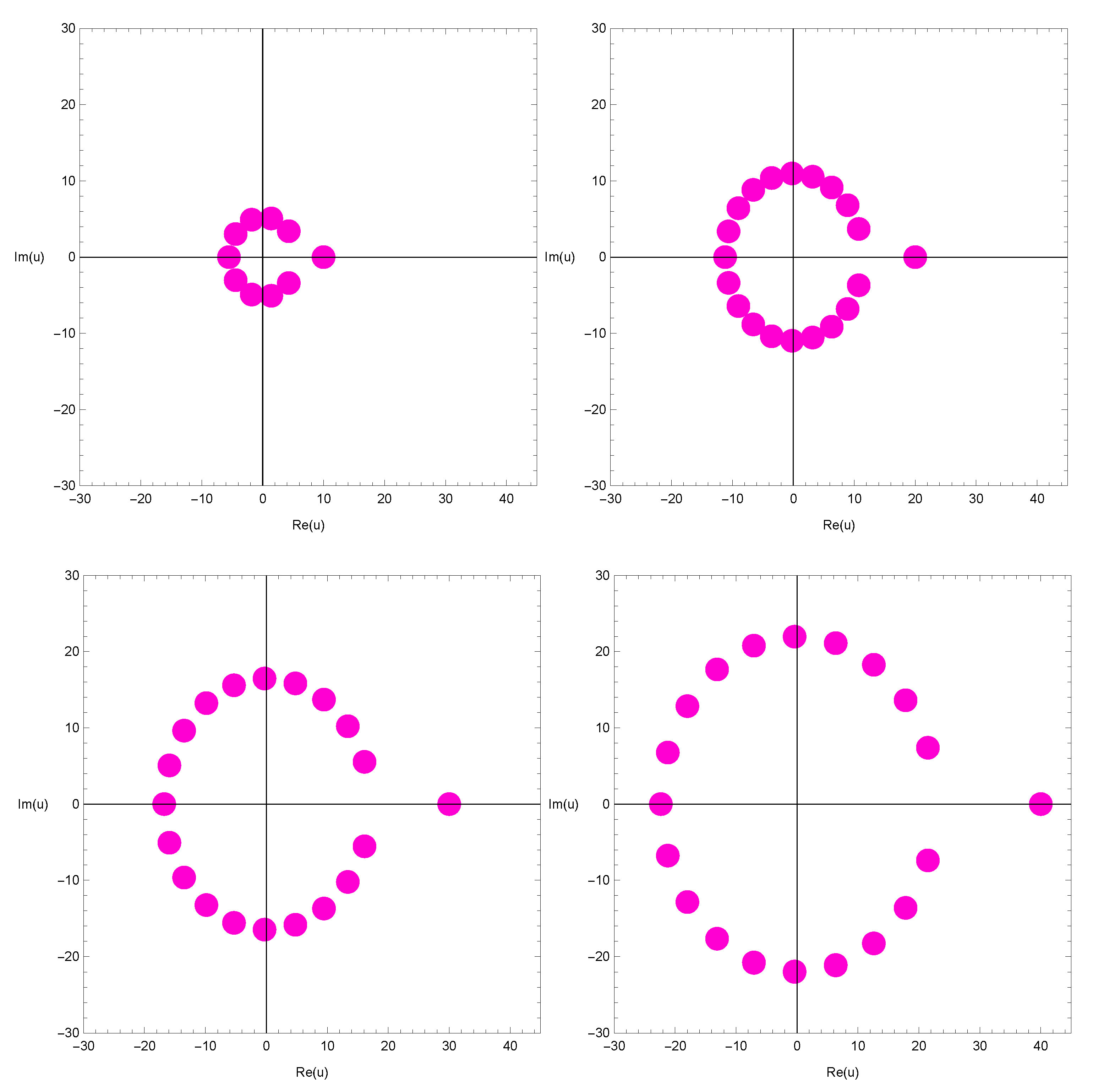
We investigated the beautiful zeros of the qGTBP ${}_{C}B_{n,q}^{\left(m\right)}(u,v)=0$ by using a computer. The zeros of the qGTBP ${}_{C}B_{n,q}^{\left(m\right)}(u,v)=0$ for $u\in \mathbb{C}$ are plotted in Figure 2.

In Figure 2 (top-left), we choose $n=10,m=10,q=-1/3$, and $v=2$. In Figure 2 (top-right), we choose $n=20,m=20,q=-1/3$, and $v=2$. In Figure 2 (bottom-left), we choose $n=20,m=30,q=-1/3$, and $v=2$. In Figure 2 (bottom-right), we choose $n=20,m=40,q=-1/3$, and $v=2$.

Using computers, several values of n were verified. However, it remains unknown whether the following conjecture is true or false for all values of n (see Table 5 and Table 6 and Figure 2).

Conjecture 1.

For $b\in \mathbb{R}$, prove that ${}_{C}B_{n,q}^{\left(m\right)}(u,b),u\in \mathbb{C}$, has $Im\left(u\right)=0$ reflection symmetry. However, ${}_{C}B_{n,q}^{\left(m\right)}(u,b)$ has no $Re\left(u\right)=a$ reflection symmetry for $a\in \mathbb{R}$.

Conjecture 2.

For $b\in \mathbb{R}$, prove that qGTBP ${}_{C}B_{n,q}^{\left(m\right)}(u,b)=0$ has n distinct solutions.

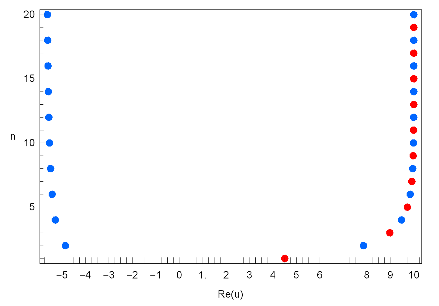
Stacks of zeros of qGTBP ${}_{C}B_{n,q}^{\left(m\right)}(u,v)=0$ for $v=2,m=10,q=-1/3$ and $1\le n\le 20$ form a 3-D structure and are presented in Figure 3. Next, we plot the real zeros of the qGTBP ${}_{C}B_{n,q}^{\left(m\right)}(u,v)=0$ for $u\in \mathbb{R},v=2,m=10,q=-1/3$ and $1\le n\le 20$ in Figure 4.

The qGTEP ${}_C\epsilon _{n,q}^{\left(m\right)}(u,v)$ can be determined explicitly. A few of them are as follows:

$$\begin{array}{l}{}_C\epsilon _{0,q}^{\left(m\right)}(u,v)=1,\\ {}_C\epsilon _{1,q}^{\left(m\right)}(u,v)=-{\displaystyle \frac{1}{2}}-{\displaystyle \frac{m}{2}}+u+v,\\ \begin{array}{ll}{}_C\epsilon _{2,q}^{\left(m\right)}(u,v)& =-{\displaystyle \frac{1}{2}}-{\displaystyle \frac{m^2}{2}}+u^2+q{v}^2+{\displaystyle \frac{1}{4{\left[2\right]}_q}}+{\displaystyle \frac{m{\left[2\right]}_q}{4}}+{\displaystyle \frac{m^2{\left[2\right]}_q}{4}}-{\displaystyle \frac{u{\left[2\right]}_q}{2}}-{\displaystyle \frac{mu{\left[2\right]}_q}{2}}\\ & -{\displaystyle \frac{v{\left[2\right]}_q}{2}}-{\displaystyle \frac{mv{\left[2\right]}_q}{2}}+uv{\left[2\right]}_q,\end{array}\\ \begin{array}{ll}{}_C\epsilon _{3,q}^{\left(m\right)}(u,v)& =-{\displaystyle \frac{1}{2}}-{\displaystyle \frac{m^3}{2}}+u^3+q^3{v}^3-{\displaystyle \frac{{\left[3\right]}_q}{8}}-{\displaystyle \frac{m{\left[3\right]}_q}{8}}-{\displaystyle \frac{m^2{\left[3\right]}_q}{8}}-{\displaystyle \frac{m^3{\left[3\right]}_q}{8}}+{\displaystyle \frac{u{\left[3\right]}_q}{4}}\\ & +{\displaystyle \frac{mu{\left[3\right]}_q}{4}}+{\displaystyle \frac{m^{2}u{\left[3\right]}_q}{4}}+{\displaystyle \frac{v{\left[3\right]}_q}{4}}+{\displaystyle \frac{mv{\left[3\right]}_q}{4}}+{\displaystyle \frac{m^{2}v{\left[3\right]}_q}{4}}-{\displaystyle \frac{uv{\left[3\right]}_q}{2}}-{\displaystyle \frac{muv{\left[3\right]}_q}{2}}\\ & +{\displaystyle \frac{{\left[3\right]}_q}{2{\left[2\right]}_q}}+{\displaystyle \frac{m{\left[3\right]}_q}{4{\left[2\right]}_q}}+{\displaystyle \frac{m^2{\left[3\right]}_q}{4{\left[2\right]}_q}}+{\displaystyle \frac{m^3{\left[3\right]}_q}{2{\left[2\right]}_q}}-{\displaystyle \frac{u{\left[3\right]}_q}{2{\left[2\right]}_q}}-{\displaystyle \frac{m^{2}u{\left[3\right]}_q}{2{\left[2\right]}_q}}-{\displaystyle \frac{u^2{\left[3\right]}_q}{2{\left[2\right]}_q}}-\\ & +{\displaystyle \frac{m{u}^2{\left[3\right]}_q}{2{\left[2\right]}_q}}-{\displaystyle \frac{v{\left[3\right]}_q}{2{\left[2\right]}_q}}-{\displaystyle \frac{m^{2}v{\left[3\right]}_q}{2{\left[2\right]}_q}}+{\displaystyle \frac{u^{2}v{\left[3\right]}_q}{{\left[2\right]}_q}}-{\displaystyle \frac{q{v}^2{\left[3\right]}_q}{2{\left[2\right]}_q}}-{\displaystyle \frac{mq{v}^2{\left[3\right]}_q}{2{\left[2\right]}_q}}+{\displaystyle \frac{qu{v}^2{\left[3\right]}_q}{{\left[2\right]}_q}}.\end{array}\end{array}$$

We display the shapes of the qGTEP ${}_C\epsilon _{n,q}^{\left(m\right)}(u,v)$ and investigate its zeros. We plot the graph of qGTEP ${}_C\epsilon _{n,q}^{\left(m\right)}(u,v)$ for $n=1,2,3,\cdots ,10$ combined together. The shape of qGTEP ${}_C\epsilon _{n,q}^{\left(m\right)}(u,v)$ for $-5\le u\le 5,v=2,m=3$, and $q=1/3$ are displayed in Figure 5.

We observed a remarkable regular structure of zeros of the qGTBP ${}_{C}B_{n,q}^{\left(m\right)}(u,v)=0$ and hope to verify the same kind of remarkable regular structure of zeros of the qGTEP ${}_C\epsilon _{n,q}^{\left(m\right)}(u,v)=0$. Our numerical results for the number of real and complex zeros of the qGTEP ${}_C\epsilon _{n,q}^{\left(m\right)}(u,v)$ are listed in

Table 7. Numbers of real and complex zeros of ${}_C\epsilon _{n,q}^{\left(m\right)}(u,v)$.

Degree n	Number of Real Zeros	Number of Complex Zeros
1	1	0
2	2	0
3	3	0
4	2	2
5	3	2
6	4	2
7	5	2
8	4	4
9	5	4
10	2	8

for $v=2,m=3$, and $q=1/3$.

Next, we calculated an approximate solution satisfying the qGTEP ${}_C\epsilon _{n,q}^{\left(m\right)}(u,v)=0$ for $u\in \mathbb{R}$, $v=2,m=3$, and $q=1/3$. The results are given in

Table 8. Approximate solutions of ${}_C\epsilon _{n,q}^{\left(m\right)}(u,v)=0$ for $u\in \mathbb{R}$.

Degree n	u
1	0
2	−2.1602,    2.1602
3	−2.1498,    −0.73464,    2.8845
4	0.30406,    3.0659
5	−2.0953,    1.0226,    3.0658
6	−1.9820,    1.4174,    3.0287
7	−1.9583,    −1.2749,    −0.42473,    1.5804,    3.0043
8	−2.0338,    0.48493,    1.5889,    2.9970
9	−1.9779,    −1.4188,    1.0634,    1.4592,    2.9975

.

We investigate the beautiful zeros of the qGTEP ${}_C\epsilon _{n,q}^{\left(m\right)}(u,v)=0$ by using a computer. The zeros of the qGTEP ${}_C\epsilon _{n,q}^{\left(m\right)}(u,v)=0$ for $u\in \mathbb{C}$ are displayed in Figure 6.

In Figure 6 (top-left), we choose $n=20,m=10,q=1/3$, and $v=2$. In Figure 6 (top-right), we choose $n=20,m=20,q=1/3$, and $v=2$. In Figure 6 (bottom-left), we choose $n=20,$$m=30$, $q=1/3$, and $v=2$. In Figure 6 (bottom-right), we choose $n=20,m=40,q=1/3$, and $v=2$.

Stacks of zeros of ${}_C\epsilon _{n,q}^{\left(m\right)}(u,v)=0$ for $v=2,m=10,q=1/3$, and $1\le n\le 26$ form a 3-D structure and are presented in Figure 7.

Next, we plot the real zeros of the qGTEP ${}_C\epsilon _{n,q}^{\left(m\right)}(u,v)=0$ for $u\in \mathbb{R},v=2,m=10,q=1/3$, and $1\le n\le 26$ in Figure 8.

From all the numerical computations done in this research work, we give the following conjectures:

Conjecture 3.

For $b\in \mathbb{R}$, prove that ${}_C\epsilon _{n,q}^{\left(m\right)}(u,b),u\in \mathbb{C}$, has $Im\left(u\right)=0$ reflection symmetry. However, ${}_C\epsilon _{n,q}^{\left(m\right)}(u,b)$ has not $Re\left(u\right)=a$ reflection symmetry for $a\in \mathbb{R}$.

Conjecture 4.

For $b\in \mathbb{R}$, prove that qGTEP ${}_C\epsilon _{n,q}^{\left(m\right)}(u,b)=0$ has n distinct solutions.

Using computers, several values of n have been verified. However, it is still remains unknown if these conjectures hold true or not for any value of n (see Table 7 and Table 8 and Figure 6). We expect that the research in this direction will be a new approach using numerical methods for the study of the qGTAP ${}_{C}A_{n,q}^{\left(m\right)}(u,v)$.

References

- Andrews, G.E.; Askey, R.; Roy, R. Special Functions—Encyclopedia of Mathematics and its Applications; Cambridge University Press: Cambridge, UK; London, UK; New York, NY, USA, 2000; Volume 71. [Google Scholar]
- Bildirici, C.; Acikgoz, M.; Araci, S. A note on analogues of tangent polynomials. J. Algebra Number Theory Acad. 2014, 4, 21. [Google Scholar]
- Ryoo, C.S. Generalized Tangent numbers and polynomials associated with p-adic integral on zp. Appl. Math. Sci. 2013, 7, 4929–4934. [Google Scholar] [CrossRef]
- Ryoo, C.S. A note on the tangent numbers and polynomials. Adv. Studies Theor. Phys. 2013, 7, 447–454. [Google Scholar] [CrossRef]
- Yasmin, G.; Muhyi, A. Certain results of 2-variable q-generalized tangent-Apostol type polynomials. J. Math. Computer Sci. 2020, in press. [Google Scholar]
- Mahmudov, N.I. On a class of q-Bernoulli and q-Euler polynomials. Adv. Difference Equ. 2013, 2013, 108. [Google Scholar] [CrossRef] [Green Version]
- Ryoo, C.S. Some properties of two dimensional q-tangent numbers and polynomials. Glob. J. Pure Appl. Math. 2016, 12, 2999–3007. [Google Scholar]
- Appell, P. Sur une Classe de Polynômes; Gauthier-Villars: Paris, France, 1880. [Google Scholar]
- Al-Salam, W.A. q-Appell polynomials. Ann. Mat. Pura Appl. 1967, 77, 31–45. [Google Scholar] [CrossRef]
- Keleshteri, M.E.; Mahmudov, N.I. A study on q-Appell polynomials from determinantal point of view. Appl. Math. Comput. 2015, 260, 351–369. [Google Scholar] [CrossRef] [Green Version]
- Al-Salam, W.A. q-Bernoulli numbers and polynomials. Math. Nachr. 1958, 17, 239–260. [Google Scholar] [CrossRef]
- Ernst, T. q-Bernoulli and q-Euler polynomials, an umbral approach. Int. J. Difference Equ. 2006, 1, 31–80. [Google Scholar]
- Yasmin, G.; Muhyi, A.; Araci, S. Certain results of q-Sheffer-Appell polynomials. Symmetry 2019, 11, 159. [Google Scholar] [CrossRef] [Green Version]
Figure 1.
Curve of qGTBP .
Figure 2.
Zeros of qGTBP .
Figure 3.
Stacks of zeros of qGTBP .
Figure 4.
Real zeros of .
Figure 5.
Curve of qGTEP .
Figure 6.
Zeros of qGTEP .
Figure 7.
Stacks of zeros of .