A Hybrid Forward–Backward Algorithm and Its Optimization Application

Abstract

In this paper, we study a hybrid forward–backward algorithm for sparse reconstruction. Our algorithm involves descent, splitting and inertial ideas. Under suitable conditions on the algorithm parameters, we establish a strong convergence solution theorem in the framework of Hilbert spaces. Numerical experiments are also provided to illustrate the application in the field of signal processing.

1. Introduction

Let H be a real Hilbert space. $\langle ·,·\rangle$ denotes the associated scalar product and $\parallel ·\parallel$ stands for the induced norm. Recall that a set-valued operator $G:H\to 2^H$ is said to be maximally monotone iff $\langle x-x^{{}^{\prime }},y-y^{{}^{\prime }}\rangle \ge 0,$$\forall y\in G\left(x\right),y^{{}^{\prime }}\in G\left(x^{{}^{\prime }}\right),$ and its graph, denoted by $\mathrm{gph}G:=\left\{\right(x,y)\in H\times H|y\in G\left(x\right)\}$, is not properly contained in the graph of any other monotone operator on H.

A fundamental and classical problem is to find a zero of a maximally monotone operator G in a real Hilbert space H, namely

$$\mathrm{find}x\in H\mathrm{such}\mathrm{that}0\in G\left(x\right).$$

(1)

This problem includes, as special cases, bifunction equilibrium problems, convex-concave saddle-point problems, minimization problems, non-smooth variational inequalities, etc. Due to its diverse applications in economics, medicine, and engineering, the techniques and methods for solving (1) have received much attention in the optimization community, see [1,2,3,4]. Indeed, the interdisciplinary nature of Problem (1) is evident from the viewpoint of algorithmic developments; see, for instance, [5,6,7,8] and the references therein. Among them, a celebrated method for solving (1) is the following proximal point algorithm. It can be traced back to the early results obtained in [6,7,8,9]. Given the current iterate $p_n$, calculate the next iterate $p_{n+1}$ via

$$p_{n+1}={(Id+{\gamma }_{n}G)}^{-1}{p}_n,\forall n\in N,$$

(2)

where $Id$ stands for the identity operator and ${\gamma }_n$ is a positive real number. The operator ${(Id+{\gamma }_{n}G)}^{-1}$ is the so-called resolvent operator, which was introduced by Moreau in [8]. In the context of algorithms, the resolvent operator is often referred as the backward operator. In [7], Rockefeller studied the operator and proved that the sequence generated by algorithm (2) is weakly convergent via the inexact evaluation of the resolvent operator in the framework of infinite-dimensional real Hilbert spaces. However, the evaluation error has to satisfy a summability restriction. Indeed, this restriction essentially implies that the resolvent operator is computed with the increasing accuracy. In fact, due to the computation of the resolvent operator is often hard to control in practice situation, this is still somewhat limiting. Quite often, computing the resolvent of a maximally monotone operator, which is an inverse problem, is not easy in many cases. Thus, this limits the practicability of the proximal point algorithm in its plain form. Aiming at this, a favorable situation occurs when the operator G can be written as the sum of two operators. Precisely, let us define $G=A+B$ such that the resolvent ${(Id+\alpha A)}^{-1}$ (implicit, backward step), and the evaluation of B (explicit, forward step) are much easier to compute than the full resolvent ${(Id+\alpha G)}^{-1}$. In so doing, we only consider the following inclusion problem: find a zero of an additively structured operator $A+B$, acting on space H, namely

$$\mathrm{find}x\in H\mathrm{such}\mathrm{that}0\in Ax+Bx,$$

(3)

where B is a smooth operator for which we can use direct evaluations, and A is a proxfriendly operator for which we can compute the resolvent. For solving (3), Lions and Mercier [10] proposed the forward–backward splitting method. It is based on the recursive application of a forward step with respect to B, followed by a backward step with respect to A. For any initial data $p_0\in H$,

$$p_{n+1}={(Id+{\gamma }_{n}A)}^{-1}(p_n-{\gamma }_{n}B{p}_n),\forall n\in \mathbb{N},$$

where $Id$ stands for the identity operator and ${\gamma }_n>0$. Basically, the operator $A:H\to 2^H$ is maximally monotone, and the operator B is $\kappa$-cocoercive (i.e., $\exists \kappa >0$ such that $\langle Bx-By,x-y\rangle \ge {\rho \parallel Bx-By\parallel }^2,\forall x,y\in H$) and $\iota$-Lipschitz continuous (i.e., $\exists \iota >0$ such that $\parallel Bx-By\parallel \le \iota \parallel x-y\parallel ,\forall x,y\in H$). It was proven that the generated sequence ${\left(p_n\right)}_{n\ge 0}$ converges weakly to a solution of (3). Of course, the problem decomposition is not the only consideration, the convergence rate is another. Accelerating first-order method is a subject of active research, which has been extensively studied. Since Polyak [6] introduced the so-called heavy ball method for minimizing a smooth convex function, much has been done on the development of first-order accelerated methods; see [11,12,13,14,15]. The inertial nature of the first-order accelerated method can be exploited in numerical computations to accelerate the trajectories and speed up the rate of convergence. In the context of algorithms, it is often referred as the inertial extrapolation, which involves two iterative steps and the second iterative step is defined based on the previous two iterates. In [16], Alvarez and Attouch employed the first-order accelerated method to study an initial proximal point algorithm for solving the problem of finding zero of a maximally monotone operator. This iteration can be written as the following form: for any initial data $p_0,p_1\in H$,

$$\begin{array}{cc}\hfill & p_{n+1}={(Id+{\lambda }_{n}G)}^{-1}(p_n+{\alpha }_n(p_n-p_{n-1})),\hfill \end{array}$$

(4)

where $Id$ stands for the identity operator, G is a maximally monotone operator, the parameters ${\left({\lambda }_n\right)}_{n\ge 0}\subset (0,\infty )$, ${\left({\alpha }_n\right)}_{n\ge 0}\subset [0,1]$, ${\sum }_{n=1}^{\infty }{\alpha }_n{\parallel p_n-p_{n-1}\parallel }^2<\infty$. It was showed that the iterative sequence ${\left(p_n\right)}_{n\ge 0}$ generated by (4) converges to a solution of inclusion Problem (1) weakly. An alternative modification to the inertial forward–backward splitting algorithm or its modifications is the following algorithm proposed by Lorenz and Pock [17]. The algorithm weakly converges to a zero of the sum of two maximally monotone operators, with one of two operators being Lipschitz continuous and single valued. Starting with any data $p_0,p_1\in H$, we define a sequence ${\left(p_k\right)}_{k\ge 0}$ as

$$\left\{\begin{array}{c}{w}_n=p_n+{\alpha }_n(p_n-p_{n-1}),\hfill \\ p_{n+1}={(M+{\gamma }_{n}A)}^{-1}(M-{\gamma }_{n}B)w_n,\hfill \end{array}\right.$$

where M is a positive definite and linear self-adjoint operator that can be used as a preconditioner for the scheme, ${\gamma }_n$ is a step-size parameter and ${\alpha }_n\in [0,1)$ is an extrapolation factor. The algorithm keeps the weak convergence property of the iterates. To motivate the so-called the inertial forward–backward splitting algorithm, we consider the following differential equation

$$\ddot{p}\left(t\right)+\iota \left(t\right)\dot{p}\left(t\right)+M_{A,B,\gamma }\left(p\left(t\right)\right)=0,$$

(5)

where $A:H\to H$ and $B:H\to H$ are operators, $M_{A,B,\gamma }:H\to H$ is the operator defined by

$$M_{A,B,\gamma }\left(p\right)=\frac{1}{\gamma }{(Id+\gamma A)}^{-1}(p-\gamma B\left(p\right))).$$

It comes naturally by discretizing the continuous dynamics (5) explicitly with a time step $h_n>0$. Set $t_n={\sum }_{i=1}^n{h}_i,{\iota }_n=\iota \left(t_n\right)$, ${\gamma }_n=\gamma \left(t_n\right)$ and $p_n=p\left(t_n\right)$. An explicit finite-difference scheme for (5) with centered second-order variation gives that

$$\frac{1}{h_n^2}(p_{n+1}-2p_n+p_{n-1})+\frac{{\iota }_n}{h_n}(p_n-p_{n-1})+M_{A,B,{\gamma }_n}\left(w_n\right)=0,$$

(6)

where $w_n$ is a point in the line passing through $p_{n-1}$ and $p_n$ (we have some flexibility for the choice of $w_n$). The above equality (6) can be rewritten as

$$p_{n+1}=\left(1-\frac{h_n^2}{{\gamma }_n}\right)(p_n+(1-{\iota }_n{h}_n)(p_n-p_{n-1}))+\frac{h_n^2}{{\gamma }_n}{(I+{\gamma }_{n}A)}^{-1}(y_n-{\gamma }_{n}B\left(w_n\right)).$$

(7)

Set ${\gamma }_n=h_n^2$ and ${\alpha }_n=1-{\iota }_n{h}_n$ in (7). With the aid of the classical Nesterov extrapolation choice for $w_n$, continuous dynamics (5) leads to a special case of the algorithm as

$$\left\{\begin{array}{c}{w}_n=p_n+{\alpha }_n(p_n-p_{n-1}),\hfill \\ p_{n+1}={(I+{\gamma }_{n}A)}^{-1}(w_n-{\gamma }_{n}B\left(w_n\right)),\hfill \end{array}\right.$$

(8)

where ${\gamma }_n$ is a step-size parameter and ${\alpha }_n$ is an extrapolation factor, the extrapolation term ${\alpha }_n(p_n-p_{n-1})$ is intended to speed up the rate of convergence. In so doing, this dynamical approach leads to a special case of the forward–backward algorithm of inertial type.

Consider the following monotone variational inequality problem (VIP, in short), which consists of finding $z\in \Omega$ such that

$$\langle S\left(z\right),x-z\rangle \ge 0,\forall x\in \Omega ,$$

(9)

where $S:\Omega \to H$ is a monotone operator. We denote the solution set of the variational inequality problem by $VI(\Omega ,S)$.

Remark 1.

It is known that x solves the $VI(\Omega ,S)$ iff x is an equilibrium point of the following dynamical system, i.e.,

$$x=Pro{j}_{\Omega }(x-\mu Sx),\mu >0,$$

where $Pro{j}_{\Omega }$ is the nearest point (or metric) projection from H onto Ω.

Variational inequality problems, which serve as a powerful mathematical model, unify several important concepts in applied mathematics, such as systems of nonlinear equations, complementarity problems, and equilibrium problems under a general and unified framework [18,19,20]. Recently, spotlight has been shed on developing efficient and implementable iterative schemes for solving monotone variational inequality problems, see [21,22,23,24]. A significant body of the work on iteration methods for VIPs has accumulated in the literature recently. In 2001, Yamada [25] investigated a so-called hybrid steepest descent method. Given the current iterate $p_n$, calculate the next iterate $p_{n+1}$ via

$$p_{n+1}=(I-\alpha {\chi }_{n}S)T{p}_n,\forall n\ge 0,$$

where the operator $T:\Omega \to H$ is nonexpansive, the operator S is $\iota$-Lipschitz continuous for some $\iota \ge 0$ and $\kappa$-strongly monotone (i.e., $\exists \kappa >0$ such that $\langle Sx-Sy,x-y\rangle \ge {\rho \parallel x-y\parallel }^2,\forall x,y\in H$), while the parameters $\alpha \in (0,2\kappa /{\iota }^2)$, ${\left({\chi }_n\right)}_{n\ge 0}\in (0,1]$, ${lim}_{n\to \infty }{\chi }_n=0$ and ${\sum }_{n=1}^{\infty }{\chi }_n=\infty$. In this paper, the set $\Omega$ can be regarded as the solution set of the inclusion problem. In continuous case, Attouch and Mainǵe [26] developed a second-order autonomous system with a Tikhonov-like regularizing term $\nabla F$, which reads

$$\left\{\begin{array}{c}\ddot{p}\left(t\right)+\alpha \dot{p}\left(t\right)+\nabla \varphi \left(p\left(t\right)\right)+B\left(p\left(t\right)\right)+\beta \left(t\right)\nabla F\left(p\left(t\right)\right)=0,\hfill \\ p\left(0\right)=p_0,\dot{p}\left(0\right)=q_0,\hfill \end{array}\right.$$

(10)

where $\alpha >0$ and $(p_0,q_0)\in H^2$ is an arbitrarily given initial data. With the assumptions: (i) $F:H\to R$ is a convex, differentiable operator with $\nabla F$ strongly monotone and Lipschitz continuous; (ii) $\varphi :H\to R$ is a convex, differentiable operator with $\nabla \varphi :H\to H$ Lipschitz continuous; (iii) $B:H\to H$ is a maximally monotone and cocoercive operator; (iv) $\beta :[0,+\infty )\to (0,+\infty )$ is a positive and decreasing function of class $C^1$ such that ${\int }_0^{+\infty }\beta \left(t\right)dt=+\infty$ and $\beta \left(t\right)\to 0$ as $t\to +\infty$, with $\dot{\beta }$ Lipschitz continuous and bounded, they proved that each trajectory of (10) strongly converges to $p^{*}$ as $t\to \infty$, which solves the following variational inequality problem:

$$\mathrm{find}{p}^{*}\in {(B+\nabla \varphi )}^{-1}\left(0\right)\mathrm{such}\mathrm{that}\langle \nabla F\left(p^{*}\right),q-p^{*}\rangle \ge 0,q\in {(B+\nabla \varphi )}^{-1}\left(0\right).$$

In the spirit of the splitting forward–backward method and the hybrid steepest descent method, we present an iterative scheme as a new strategy, parallel to that of the autonomous system (10). We analyze the convergence with the underlying operator B cocoercive and the extension from condition (ii) to the general maximally monotone case, which is considered in Section 3. From this perspective, our study is the natural extension of the convergence results obtained by Attouch and Mainǵe [26] in the case of continuous dynamical systems.

2. Preliminaries

Lemma 1

([25]). Suppose that $W:H\to \mathbb{R}$ is Fr$\acute{e}$chet differentiable with $\nabla W:H\to H$ being κ-strongly monotone and ι-Lipschitz continuous. Define $S:=Id-\chi \alpha \nabla W$, where $\chi \in [0,1]$ and $\alpha \in (0,2\kappa /{\iota }^2)$. Then $\parallel S\left(x\right)-S\left(y\right)\parallel \le (1-\chi \vartheta )\parallel x-y\parallel (x,y\in H)$, where $\vartheta :=1-\sqrt{1-\alpha (2\kappa -\alpha {\iota }^2)}\in (0,1]$.

Lemma 2

([27]). If $B:H\to H$ is a ρ-cocoercive operator, then

(i) 

B is a $\frac{1}{\rho }$-Lipschitz continuous and monotone operator;

(ii) 

if ν is any constant in $(0,2\rho ]$, then $Id-\nu B$ is nonexpansive, where $Id$ stands for the identity operator on H.

Lemma 3.

Let H be a Hilbert space, $A:H\to 2^H$ be a maximally monotone operator and $B:E\to E$ be a κ-cocoercive on H. Then

(i) 

$${\parallel (Id+sA)}^{-1}{(Id-sB)x-x\parallel \le 2\parallel (Id+tA)}^{-1}(Id-tB)x-x\parallel ,\forall x\in H,$$

where t and s are any positive real numbers with $t\ge s.$

(ii) 

${(A+B)}^{-1}\left(0\right)=Fix\left({(Id+\lambda A)}^{-1}(Id-\lambda B)\right)$, $\forall \lambda >0$.

Proof. 

Since A is maximally monotone, one has

$$\begin{array}{c}\langle {(Id+sA)}^{-1}(Id-sB)x-{(Id+tA)}^{-1}(Id-tB)x,\\ \frac{x-{(Id+sA)}^{-1}(Id-sB)x}{s}-\frac{x-{(Id+tA)}^{-1}(Id-tB)x}{t}\rangle \ge 0.\end{array}$$

 □

Lemma 4

([28]). Let S be a nonexpansive mapping defined on a closed convex subset C of a Hilbert space H. Then $Id-S$ is demi-closed, i.e., whenever ${\left(x_n\right)}_{n\ge 0}$ is a sequence in C weakly converging to some $x\in C$ and the sequence ${\left((Id-S)x_n\right)}_{n\ge 0}$ strongly converges to some $y\in H$, it follows that $y=(Id-S)x$.

Lemma 5

([29]). Let ${\left({\mu }_n\right)}_{n\ge 0}$ be a sequence of nonnegative real numbers such that

$${\mu }_{n+1}\le (1-{\lambda }_n){\mu }_n+{\lambda }_n{\nu }_n+{\gamma }_n,$$

where ${\left({\lambda }_n\right)}_{n\ge 0}\subset (0,1)$ and ${\left({\nu }_n\right)}_{n\ge 0}$, ${\left({\gamma }_n\right)}_{n\ge 0}$ satisfy the following conditions (i) ${lim}_{n\to \infty }{\lambda }_n=0$, ${\sum }_{n=0}^{\infty }{\lambda }_n=\infty$; (ii) ${lim\; sup}_{n\to \infty }{\nu }_n\le 0$; (iii) ${\gamma }_n\ge 0$, ${\sum }_{n=0}^{\infty }{\gamma }_n<\infty$. Then ${lim}_{n\to \infty }{u}_n=0$.

Lemma 6

([30]). Let ${\left({\zeta }_n\right)}_{n\ge 0}$ be a sequence of nonnegative real numbers such that there exists a subsequence $\left({\zeta }_{n_i}\right)$ of ${\left({\zeta }_n\right)}_{n\ge 0}$ such that ${\zeta }_{n_i+1}>{\zeta }_{n_i}$ for all $i\in \mathbb{N}$. Then there exists a nondecreasing sequence $\left(m_j\right)$ of $\mathbb{N}$ such that ${lim}_{j\to \infty }{m}_j=\infty$ and the following properties are satisfied by all (sufficiently large) number of $j\in \mathbb{N}$, ${\zeta }_{m_j+1}\ge {\zeta }_{m_j}$, ${\zeta }_{m_j+1}\ge {\zeta }_k.$ In fact, $m_j$ is the largest number n in the set $\{1,2,\cdots ,j\}$ such that ${\zeta }_{n+1}\ge {\zeta }_n$.

3. Main Results

Throughout this section, we make the following standing assumptions

Assumption 1.

(a) $Id$ stands for the identity operator. The operator $S:H\to H$ is supposed to be κ-strongly monotone and ι-Lipschitz continuous for some $\kappa ,\iota >0$;

(b) Let $A:H\to 2^H$ be a maximally monotone operator, and $B:H\to H$ be a ρ-cocoercive operator for some $\rho >0$, with the solution set $\Omega ={(A+B)}^{-1}\left(0\right)\ne \varnothing$.

Our Algorithm 1 is formally designed as follows.

Algorithm 1: The hybrid forward–backward algorithm

We make the following assumption with respect to the algorithm parameters.

Assumption 2.

($C_1$) $0<{lim\; inf}_{n\to \infty }{\nu }_n\le {lim\; sup}_{n\to \infty }{\nu }_n<2\rho$; (C${}_2$) ${\left({\eta }_n\right)}_{n\ge 0}\subset (0,1),{lim}_{n\to \infty }{\eta }_n=0,{\eta }_{n+1}=O\left({\eta }_n\right),{\sum }_{n=0}^{\infty }{\eta }_n=\infty$; (C${}_3$) ${lim}_{n\to \infty }\frac{{\mu }_n}{{\eta }_n}\parallel p_n-p_{n-1}\parallel =0$; (C${}_4$) $\delta \in (0,2\kappa /{\iota }^2)$.

Remark 2.

Please note that the condition (C${}_3$) of Assumption 2 can be easily implemented since the value of $\parallel p_n-p_{n-1}\parallel$ is known before choosing ${\mu }_n$. Indeed, the parameter ${\mu }_n$ can be chosen such that

$${\mu }_n=\left\{\begin{array}{cc}\omega ,\hfill & if{p}_n=p_{n-1};\hfill \\ {\mu }_n=\frac{{\tau }_n}{\parallel p_n-p_{n-1}\parallel },\hfill & if otherwise,\hfill \end{array}\right.$$

where $0\le \omega$ and ${\left({\tau }_n\right)}_{n\ge 0}$ is a positive sequence such that ${\tau }_n=\circ \left({\eta }_n\right)$.

Now we are in a position to state and prove the main result of this section.

Theorem 1.

Suppose that Assumptions 1, 2 hold. Then for any initial data $p_0,p_1\in H$, the weak sequential cluster point of sequences ${\left(p_n\right)}_{n\ge 0},{\left(w_n\right)}_{n\ge 0}$ and ${\left(q_n\right)}_{n\ge 0}$ generated by Algorithm 1 belongs to the solution set of Problem 3. In addition, the three sequences converge strongly to the unique element of $VI(\Omega ,S)$.

Proof. 

First, we show that $I-\delta R$ is a contraction operator. According to Lemma 1, we have

$$\begin{array}{cc}\hfill {\parallel (Id-\delta S)x-(Id-\delta S)y\parallel }^2=& {\parallel x-y\parallel }^2+{\delta }^2{\parallel Sx-Sy\parallel }^2-2\delta \langle x-y,Sx-Sy\rangle \hfill \\ \hfill \le & {\parallel x-y\parallel }^2+{\delta }^2{\iota }^2{\parallel x-y\parallel }^2-2\delta \kappa {\parallel x-y\parallel }^2\hfill \\ \hfill =& {(1-\alpha )}^2{\parallel x-y\parallel }^2,\hfill \end{array}$$

(11)

where $\alpha =\frac{1}{2}\delta (2\kappa -\delta {\iota }^2)$. Thus, we find that $Id-\delta S$ is a contraction operator with the constant $1-\alpha$. In light of the nonexpansivity of $Pro{j}_{\Omega }$, we further obtain that $Pro{j}_{\Omega }(Id-\delta S)$ is a contraction operator. From the Banach contraction principle, there exists a unique point $a\in \Lambda$ such that $a=Pro{j}_{\Omega }(Id-\delta S)a$.

Now, it remains to prove that ${\left(p_n\right)}_{n\ge 0}$ is bounded. Since $B:H\to H$ is $\rho$-cocoercive and ${(Id+{\nu }_{n}A)}^{-1}$ is firmly nonexpansive, one concludes from Lemma 2 that $Id-{\nu }_{n}B$ is nonexpansive. Let $z\in \Lambda$ be arbitrarily chosen. Invoking Assumption 2 (C${}_1$), one infers that

$$\begin{array}{cc}\hfill \parallel q_n{-z\parallel }^2& = \parallel {(Id+{\nu }_{n}A)}^{-1}(Id-{\nu }_{n}B)w_n-{(Id+{\nu }_{n}A)}^{-1}(Id-{\nu }_{n}B){z\parallel }^2\hfill \\ \hfill & \le \parallel w_n-z+{\nu }_{n}Bz-{\nu }_{n}B{w}_n{\parallel }^2\hfill \\ \hfill & \le \parallel w_n{-z\parallel }^2-{\nu }_n(2\rho -{\nu }_n){\parallel Bz-B{w}_n\parallel }^2\hfill \\ \hfill & \le \parallel w_n{-z\parallel }^2,\hfill \end{array}$$

(12)

which yields

$${\nu }_n(2\rho -{\nu }_n)\parallel Bz-B{w}_n{\parallel }^2\le \parallel w_n{-z\parallel }^2-{\parallel q_n-z\parallel }^2,$$

(13)

and

$$\parallel q_n{-z\parallel }^2\le {\parallel w_n-z\parallel }^2.$$

(14)

From the definition of $w_n$, one reaches

$$\parallel w_n-z\parallel \le \parallel p_n-z\parallel +{\mu }_n\parallel p_n-p_{n-1}\parallel .$$

(15)

Invoking Assumption 2 (C${}_3$), there exists a positive constant $M_1\in \mathbb{R}$ such that

$$\begin{array}{c}\hfill \frac{{\mu }_n}{{\eta }_n}\parallel p_n-p_{n-1}\parallel \le M_1,\forall n\ge 0.\end{array}$$

(16)

From the definition of $p_n$, which together with (14)–(16), one obtains

$$\begin{array}{cc}\hfill \parallel p_{n+1}-z\parallel & = \parallel (Id-\delta {\eta }_{n}S)q_n-(Id-\delta {\eta }_{n}S)z-\delta {\eta }_{n}Sz\parallel \hfill \\ \hfill & \le (1-\xi {\eta }_n)\parallel w_n-z\parallel +\delta {\eta }_n\parallel Sz\parallel \hfill \\ \hfill & \le (1-\xi {\eta }_n)(\parallel p_n-z\parallel +{\eta }_n{M}_1)+\delta {\eta }_n\parallel Sz\parallel \hfill \\ \hfill & \le max\left\{\parallel p_n-z\parallel ,\frac{1}{\xi }(M_1+\delta \parallel Sz\parallel )\right\}\hfill \\ \hfill & \cdots \hfill \\ \hfill & \le max\left\{\parallel p_1-z\parallel ,\frac{1}{\xi }(M_1+\delta \parallel Sz\parallel )\right\},\hfill \end{array}$$

(17)

where $\xi =1-\sqrt{1-\delta (2\kappa -\delta {\iota }^2)}\in (0,1]$, due to Assumption 2 $\left(C_4\right)$. This implies that sequence ${\left(p_n\right)}_{n\ge 0}$ is bounded. At the same time, by putting together (14) and (15), one concludes that ${\left(q_n\right)}_{n\ge 0}$ and ${\left(w_n\right)}_{n\ge 0}$ are bounded. Once again, using the definition of $w_n$, one concludes that

$$\begin{array}{cc}\hfill \parallel w_n{-z\parallel }^2& \le \parallel p_n{-z\parallel }^2+{\mu }_n\parallel p_n-p_{n-1}\parallel ({\mu }_n\parallel p_n-p_{n-1}\parallel +2\parallel p_n-z\parallel )\hfill \\ \hfill & \le \parallel p_n{-z\parallel }^2+\frac{{\mu }_n}{{\eta }_n}\parallel p_n-p_{n-1}\parallel M_2,\hfill \end{array}$$

(18)

where

$$M_2=\underset{n\ge 0}{sup}{\eta }_n({\mu }_n\parallel p_n-p_{n-1}\parallel +2\parallel p_n-z\parallel )<\infty .$$

(19)

By combining (12) with (18), one immediately concludes that

$$\begin{array}{cc}\hfill \parallel q_n{-z\parallel }^2& \le \parallel p_n{-z\parallel }^2+\frac{{\mu }_n}{{\eta }_n}\parallel p_n-p_{n-1}\parallel M_2-{\nu }_n(2\kappa -{\nu }_n){\parallel Bz-B{w}_n\parallel }^2.\hfill \end{array}$$

(20)

Invoking (20), which together with the definition of $p_n$, one deduces that

$$\begin{array}{cc}\hfill \parallel p_{n+1}{-z\parallel }^2=& (Id-\xi {\eta }_n){\parallel q_n-z\parallel }^2-2\delta {\eta }_n\langle p_{n+1}-z,Sz\rangle \hfill \\ \hfill \le & \parallel p_n{-z\parallel }^2+\frac{{\mu }_n}{{\eta }_n}\parallel p_n-p_{n-1}\parallel M_2-{\nu }_n(2\kappa -{\nu }_n){\parallel Bz-B{w}_n\parallel }^2+{\eta }_n{M}_3,\hfill \end{array}$$

(21)

where $M_3={sup}_{n\ge 0}2\delta \langle z-p_{n+1},Sz\rangle <\infty$, due to the boundedness of ${\left(p_n\right)}_{n\ge 0}$. Let us rewrite (21) as

$$\begin{array}{cc}\hfill {\nu }_n(2\kappa -{\nu }_n){\parallel Bz-B{w}_n\parallel }^2\le & \parallel p_n{-z\parallel }^2-\parallel p_{n+1}{-z\parallel }^2+\frac{{\mu }_n}{{\eta }_n}\parallel p_n-p_{n-1}\parallel M_2+{\eta }_n{M}_3.\hfill \end{array}$$

(22)

By using the firmly nonexpansive property of ${(Id+{\nu }_{n}A)}^{-1}$, one arrives at

$$\begin{array}{cc}\hfill \parallel q_n{-z\parallel }^2\le & \langle q_n-z,(Id-{\nu }_{n}B)w_n-(Id-{\nu }_{n}B)z\rangle \hfill \\ \hfill =& \frac{1}{2}\parallel q_n{-z\parallel }^2+\frac{1}{2}{\parallel (Id-{\nu }_{n}B)w_n-(Id-{\nu }_{n}B)z\parallel }^2\hfill \\ \hfill & -\frac{1}{2}{\parallel (q_n-z)-(Id-{\nu }_{n}B)w_n+(Id-{\nu }_{n}B)z\parallel }^2\hfill \\ \hfill \le & \frac{1}{2}\parallel q_n{-z\parallel }^2+\frac{1}{2}\parallel w_n{-z\parallel }^2-\frac{1}{2}\parallel q_n-w_n{\parallel }^2-\frac{{\nu }_n^2}{2}{\parallel B{w}_n-Bz\parallel }^2\hfill \\ \hfill & +{\nu }_n\parallel q_n-w_n\parallel \parallel B{w}_n-Bz\parallel ,\hfill \end{array}$$

which can be equivalently rewritten as

$$\begin{array}{cc}\hfill \parallel q_n{-z\parallel }^2\le & \parallel w_n{-z\parallel }^2-\parallel q_n-w_n{\parallel }^2-{\nu }_n^2\parallel B{w}_n{-Bz\parallel }^2+2{\nu }_n\parallel q_n-w_n\parallel \parallel B{w}_n-Bz\parallel .\hfill \end{array}$$

(23)

Returning to (14), (18) and (23), one concludes

$$\begin{array}{cc}\hfill \parallel p_{n+1}{-z\parallel }^2=& \parallel {\eta }_n(Id-\delta S)q_n+(1-{\eta }_n)q_n{-z\parallel }^2\hfill \\ \hfill =& {\eta }_n\parallel (Id-\delta S)q_n{-z\parallel }^2+(1-{\eta }_n)\parallel q_n{-z\parallel }^2-{\eta }_n(1-{\eta }_n){\parallel \delta S{q}_n\parallel }^2\hfill \\ \hfill \le & {\eta }_n\parallel (Id-\delta S)q_n{-z\parallel }^2+{\parallel q_n-z\parallel }^2\hfill \\ \hfill \le & {\eta }_n\parallel (Id-\delta S)q_n{-z\parallel }^2+\parallel p_n{-z\parallel }^2+\frac{{\mu }_n}{{\eta }_n}\parallel p_n-p_{n-1}\parallel M_2\hfill \\ \hfill & -\parallel q_n-w_n{\parallel }^2-\frac{{\nu }_n^2}{2}\parallel B{w}_n{-Bz\parallel }^2+2{\nu }_n\parallel q_n-w_n\parallel \parallel B{w}_n-Bz\parallel ,\hfill \end{array}$$

that is,

$$\begin{array}{cc}\hfill \parallel q_n-w_n{\parallel }^2 \le & {\eta }_n\parallel (Id-\delta S)q_n{-z\parallel }^2+\frac{{\mu }_n}{{\eta }_n}\parallel p_n-p_{n-1}\parallel M_2\hfill \\ \hfill & +2{\nu }_n\parallel q_n-w_n\parallel \parallel B{w}_n-Bz\parallel +\parallel p_n{-z\parallel }^2-{\parallel p_{n+1}-z\parallel }^2.\hfill \end{array}$$

(24)

Next, we show that $(\parallel p_n-z{{\parallel }^2)}_{n\ge 0}$ converges to zero by considering two possible cases on the sequence $(\parallel p_n-z{{\parallel }^2)}_{n\ge 0}$.

Case 1. There exists $N\in \mathbb{N}$ such that $\parallel p_{n+1}{-z\parallel }^2\le {\parallel p_n-z\parallel }^2,\forall n\ge N$. Recalling that $\parallel p_n{-z\parallel }^2$ is lower bounded, one deduces that ${lim}_{n\to \infty }{\parallel p_n-z\parallel }^2$ exists. Using Assumption 2 (C${}_2$), and letting n tend to infinity in (22), one finds that

$$\underset{n\to \infty }{lim}{\nu }_n\parallel Bz-B{w}_n\parallel =0.$$

(25)

Taking account of Assumption 2 (C${}_2$), (C${}_3$), (25), and letting n tend to infinity in (24), one concludes that

$$\underset{n\to \infty }{lim}{\parallel q_n-w_n\parallel }^2=0.$$

(26)

It follows from Assumption 2 (C${}_2$), (C${}_3$) the definitions of $w_n$ and $p_{n+1}$ that

$$\underset{n\to \infty }{lim}\parallel w_n-p_n\parallel =\underset{n\to \infty }{lim}{\mu }_n\parallel p_n-p_{n-1}\parallel =0,$$

(27)

and

$$\underset{n\to \infty }{lim}\parallel p_{n+1}-q_n\parallel =\underset{n\to \infty }{lim}\delta {\eta }_n\parallel R{q}_n\parallel =0.$$

(28)

Resorting to (26)–(28), one finds that

$$\underset{n\to \infty }{lim}\parallel p_{n+1}-p_n\parallel \le \underset{n\to \infty }{lim}(\parallel p_{n+1}-q_n\parallel +\parallel q_n-w_n\parallel +\parallel w_n-p_n\parallel )=0.$$

(29)

Denote $G_{{\nu }_n}={(Id+{\nu }_{n}A)}^{-1}(Id-{\nu }_{n}B)$. It is then immediately that

$$\underset{n\to \infty }{lim}\parallel G_{{\nu }_n}{w}_n-w_n\parallel =\underset{n\to \infty }{lim}\parallel q_n-w_n\parallel =0.$$

(30)

For any $\gamma \ge 0$ such that $\gamma \le {\nu }_n$, $\forall n\ge 0$, it implies from Lemma 3 that

$$\underset{n\to \infty }{lim}\parallel G_{\gamma }{w}_n-w_n\parallel \le 2\underset{n\to \infty }{lim}\parallel G_{{\nu }_n}{w}_n-w_n\parallel =0.$$

(31)

Since ${\left(p_n\right)}_{n\ge 0}$ is a bounded sequence, there exists a subsequence ${\left(p_{n_i}\right)}_{n\ge 0}$ of ${\left(p_n\right)}_{n\ge 0}$ and a weak sequential cluster point $s\in H$ such that $p_{n_i}\rightharpoonup s$ as $i\to \infty$. Due to (26) and (27), one finds that $w_{n_i}\rightharpoonup s$ and $q_{n_i}\rightharpoonup s$ as $i\to \infty$. Thus,

$$\underset{n\to \infty }{lim\; sup}\langle Sz,z-w_n\rangle =\underset{i\to \infty }{lim}\langle Sz,z-w_{n_i}\rangle .$$

(32)

From the demiclosedness of $I-G_{\gamma }$ and Lemma 4, one obtains that $s\in Fix\left(G_{\gamma }\right)$. In view of $Fix\left(G_{\gamma }\right)={(A+B)}^{-1}\left(0\right)$, one concludes $s\in \Lambda$. From the fact that $a=Pro{j}_{\Lambda }(I-\delta S)a$, one sees $\langle a-(I-\delta S)a,s-a\rangle \ge 0$. As a straightforward consequence, one finds

$$\langle Sa,a-s\rangle \le 0.$$

(33)

Coming back to (29), (32) and (33), one has

$$\underset{n\to \infty }{lim\; sup}\langle Sa,a-p_{n+1}\rangle =\underset{n\to \infty }{lim\; sup}\langle Sa,a-p_n\rangle =\underset{i\to \infty }{lim}\langle Sa,a-p_{n_i}\rangle =\langle Sa,a-s\rangle \le 0.$$

(34)

Returning to (11) and owing to the definitions of $p_n$ and $q_n$, one finds that

$$\begin{array}{cc}\hfill \parallel p_{n+1}{-a\parallel }^2=& \parallel {\eta }_n(Id-\delta S)q_n+(1-{\eta }_n)q_n{-a\parallel }^2\hfill \\ \hfill \le & {(1-{\eta }_n)}^2{\parallel q_n-a\parallel }^2+2{\eta }_n\langle (Id-\delta S)q_n-a,p_{n+1}-a\rangle \hfill \\ \hfill =& {(1-{\eta }_n)}^2{\parallel q_n-a\parallel }^2+2{\eta }_n\langle (Id-\delta S)q_n-(Id-\delta S)a+(Id-\delta S)a-a,p_{n+1}-a\rangle \hfill \\ \hfill \le & {(1-{\eta }_n)}^2\parallel q_n{-a\parallel }^2+2{\eta }_n(1-\alpha )\parallel q_n-a\parallel \parallel p_{n+1}-a\parallel +2\delta {\eta }_n\langle Sa,a-p_{n+1}\rangle \hfill \\ \hfill \le & {(1-{\eta }_n)}^2(\parallel p_n-a\parallel +{\mu }_n\parallel p_n-p_{n-1}{\parallel )}^2\hfill \\ \hfill & +2{\eta }_n(1-\alpha )(\parallel p_n{-a\parallel }^2+{\mu }_n\parallel p_n-p_{n-1}\parallel \parallel p_n-a\parallel )+2\delta {\eta }_n\langle Sa,a-p_{n+1}\rangle \hfill \\ \hfill \le & (1-2{\eta }_n\alpha )(\parallel p_n{-a\parallel }^2+2{\mu }_n\parallel p_n-p_{n-1}\parallel \parallel p_n-a\parallel )\hfill \\ \hfill & +{\mu }_n^2{\parallel p_n-p_{n-1}\parallel }^2+2\delta {\eta }_n\langle Sa,a-p_{n+1}\rangle ,\hfill \end{array}$$

(35)

where $\alpha =\frac{1}{2}\delta (2\kappa -\delta {\iota }^2)\in (0,1)$. Let

$${\Gamma }_n=\parallel p_n{-a\parallel }^2+2{\mu }_n\parallel p_n-p_{n-1}\parallel \parallel p_n-a\parallel$$

and

$$M_4=\underset{n\ge 0}{sup}\frac{{\eta }_{n+1}}{{\eta }_n\alpha }\parallel p_{n+1}-a\parallel .$$

Furthermore, due to Assumption 2 (C${}_2$) and the boundedness of ${\left(p_n\right)}_{n\ge 0}$, we find that $M_4<\infty$. In so doing, it asserts that

$$\begin{array}{cc}\hfill & {\Gamma }_{n+1}\le (1-2{\eta }_n\alpha ){\Gamma }_n+2{\eta }_n\alpha \left(\frac{\delta }{\alpha }\langle Sa,p_{n+1}-a\rangle +\left(\frac{{\mu }_{n+1}}{{\eta }_{n+1}}\parallel p_{n+1}-p_n\parallel \right)M_4+\frac{{\eta }_n}{2\alpha }{\left(\frac{{\mu }_n}{{\eta }_n}\parallel p_n-p_{n-1}\parallel \right)}^2\right).\hfill \end{array}$$

Invoking (32), we infer that

$$\underset{n\to \infty }{lim\; sup}\left(\frac{\delta }{\alpha }\langle Sa,p_{n+1}-a\rangle +\left(\frac{{\mu }_{n+1}}{{\eta }_{n+1}}\parallel p_{n+1}-p_n\parallel \right)M_4+\frac{{\eta }_n}{2\alpha }{\left(\frac{{\mu }_n}{{\eta }_n}\parallel p_n-p_{n-1}\parallel \right)}^2\right)\le 0.$$

According to Assumption 2 (C${}_2$), one finds that $2{\eta }_n\alpha \in (0,1)$ and ${lim}_{n\to \infty }2{\eta }_n\alpha =0$. So doing, Lemma 5 asserts that $\underset{n\to \infty }{lim}{\Gamma }_n=0$, which further implies that $\underset{n\to \infty }{lim}\parallel p_n-a\parallel =0$. Coming back to (26) and (27), one concludes that ${\left(p_n\right)}_{n\ge 0}$, ${\left(q_n\right)}_{n\ge 0}$, ${\left(w_n\right)}_{n\ge 0}$ converge strongly to a.

Case 2. There exists a subsequence $(\parallel p_{n_j}-z{{\parallel }^2)}_{j\ge 0}$ of $(\parallel p_n-z{{\parallel }^2)}_{n\ge 0}$ such that

$$\parallel p_{n_j}{-z\parallel }^2<{\parallel p_{n_j+1}-z\parallel }^2,\forall j\in \mathbb{N}.$$

In this case, it is obvious that there exists a nondecreasing sequence ${\left(m_k\right)}_{k\ge 0}\in \mathbb{N}$ such that $m_k\to \infty$ as $k\to \infty$. Lemma 6 asserts that the following inequalities hold,

$$\parallel p_{m_k}{-z\parallel }^2\le \parallel p_{m_k+1}{-z\parallel }^2,\parallel p_k{-z\parallel }^2\le {\parallel p_{m_k}-z\parallel }^2,\forall k\in \mathbb{N}.$$

(36)

Thanks to (21) and (36), one finds

$$\begin{array}{cc}\hfill {\nu }_n(2\kappa -{\nu }_n){\parallel Bz-B{w}_n\parallel }^2\le & {\mu }_n{M}_1\parallel p_n-p_{n-1}\parallel +M_2{\eta }_n.\hfill \end{array}$$

By letting n tend to infinity in the above inequality, one infers that ${lim}_{n\to \infty }{\nu }_n\parallel Bz-B{w}_n\parallel =0$. According to (24) and (36), one finds that

$$\begin{array}{cc}\hfill \parallel q_n-w_n{\parallel }^2\le & {\eta }_n\parallel (Id-\delta S)q_n{-z\parallel }^2+{\mu }_n{M}_1\parallel p_n-p_{n-1}\parallel +2{\nu }_n\parallel q_n-w_n\parallel \parallel B{w}_n-Bz\parallel .\hfill \end{array}$$

Accordingly, one finds that ${lim}_{n\to \infty }\parallel q_n-w_n\parallel =0$. A calculation similar to the proof in Case 1. guarantees that

$$\underset{n\to \infty }{lim}\parallel p_{m_k+1}-p_{m_k}\parallel =0,$$

and

$$\underset{k\to \infty }{lim\; sup}\langle Sa,a-p_{m_k+1}\rangle \le 0.$$

(37)

Invoking (35), one finds

$$\begin{array}{cc}\hfill \parallel p_{m_k+1}{-a\parallel }^2\le & {(1-{\eta }_{m_k})}^2(\parallel p_{m_k}-a\parallel +{\mu }_{m_k}\parallel p_{m_k}-p_{m_k-1}{\parallel )}^2+2{\eta }_{m_k}(1-\alpha )(\parallel p_{m_k}-a\parallel \hfill \\ \hfill & +{\mu }_{m_k}\parallel p_{m_k}-p_{m_k-1}\parallel )\parallel p_{m_k+1}-a\parallel +2\delta {\eta }_{m_k}\langle Sa,a-p_{m_k+1}\rangle \hfill \\ \hfill \le & {(1-{\eta }_{m_k})}^2(\parallel p_{m_k+1}-a\parallel +{\mu }_{m_k}\parallel p_{m_k}-p_{m_k-1}{\parallel )}^2+2{\eta }_{m_k}(1-\alpha )(\parallel p_{m_k+1}{-a\parallel }^2\hfill \\ \hfill & +{\mu }_{m_k}\parallel p_{m_k}-p_{m_k-1}\parallel \parallel p_{m_k+1}-a\parallel )+2\delta {\eta }_{m_k}\langle Sa,a-p_{m_k+1}\rangle \hfill \\ \hfill \le & (1-2{\eta }_{m_k}\alpha )(\parallel p_{m_k+1}{-a\parallel }^2+2{\mu }_{m_k}\parallel p_{m_k}-p_{m_k-1}\parallel \parallel p_{m_k+1}-a\parallel )\hfill \\ \hfill & +{\mu }_{m_k}^2{\parallel p_{m_k}-p_{m_k-1}\parallel }^2+2\delta {\eta }_{m_k}\langle Sa,a-p_{m_k+1}\rangle \hfill \\ \hfill \le & (1-2{\eta }_{m_k}\alpha )\parallel p_{m_k+1}{-a\parallel }^2+2{\mu }_{m_k}\parallel p_{m_k}-p_{m_k-1}\parallel \parallel p_{m_k+1}-a\parallel \hfill \\ \hfill & +{\mu }_{m_k}^2{\parallel p_{m_k}-p_{m_k-1}\parallel }^2+2\delta {\eta }_{m_k}\langle Sa,a-p_{m_k+1}\rangle ,\hfill \end{array}$$

(38)

which sends us to

$$\begin{array}{cc}\hfill \parallel p_{m_k+1}{-a\parallel }^2\le & \frac{{\mu }_{m_k}}{{\eta }_{m_k}}\parallel p_{m_k}-p_{m_k-1}\parallel M_5+{\left(\frac{{\mu }_{m_k}}{{\eta }_{m_k}}\parallel p_{m_k}-p_{m_k-1}\parallel \right)}^2{M}_6+\langle Sa,a-p_{m_k+1}\rangle M_7,\hfill \end{array}$$

(39)

where $M_5={sup}_{n\ge 0}\frac{\parallel p_{n+1}-a\parallel }{\alpha }<\infty$, $M_6={sup}_{n\ge 0}\frac{{\eta }_n}{2\alpha }<\infty$ and $M_7=\frac{\delta }{\alpha }$. By applying Assumption 2 (C${}_3$), which together with (39), we additionally derive that

$$\begin{array}{c}\hfill \underset{k\to \infty }{lim\; sup}{\parallel p_{m_k+1}-a\parallel }^2\le 0.\end{array}$$

(40)

From $\parallel p_k-a\parallel \le \parallel p_{m_k+1}-a\parallel$, we obtain that ${lim\; sup}_{k\to \infty }\parallel p_k-a\parallel =0$. This further implies that ${\left(p_k\right)}_{k\ge 0}$ converges strongly to a. Furthermore, one has

$$\underset{n\to \infty }{lim}\parallel q_n-w_n{\parallel }^2=0,\underset{n\to \infty }{lim}\parallel w_n-p_n\parallel =0.$$

(41)

Recalling that the sequence ${\left(p_k\right)}_{k\ge 0}$ converges strongly to a, which together with (41), one finds that the sequences ${\left(q_n\right)}_{n\ge 0}$ and ${\left(w_n\right)}_{n\ge 0}$ also converge strongly to a. From the above, one can conclude that the sequences generated by Algorithm 1 converge strongly to the unique solution $a\in \Omega$ such that $a=Pro{j}_{\Omega }(Id-\delta S)a$. In view of Remark 1, one sees that $a\in VI(\Omega ,S)$. Furthermore, the solution of such variational inequality is unique due to the properties of S. This completes the proof. □

If ${\left({\mu }_n\right)}_{n\in \mathbb{N}}:=0$, we obtain the following Algorithm 2 without the inertial extrapolation as a special case of Algorithm 1.

Algorithm 2: The hybrid forward–backward algorithm without the inertial term

Recently, much attention has been paid to the relationship between continuous-time systems and neural network models, see [31,32]. One can views an iterative algorithm as a time discretized version of a continuous-time dynamic system. We propose a recurrent neural network to Problem (1). By taking constant parameters, we obtain the following consequence of the dynamical with respect to the time variable t

$$\left\{\begin{array}{c}w\left(t\right)=p\left(t\right)+\alpha \dot{p}\left(t\right)),\hfill \\ u\left(t\right)={(Id+\gamma A)}^{-1}(w\left(t\right)-\gamma Bw\left(t\right)),\hfill \\ \dot{p}\left(t\right)+\ddot{p}\left(t\right)=(Id-\delta \eta \left(t\right)S)u\left(t\right),\hfill \\ p\left(0\right)=p_0,\dot{p}\left(0\right)=z_0.\hfill \end{array}\right.$$

(42)

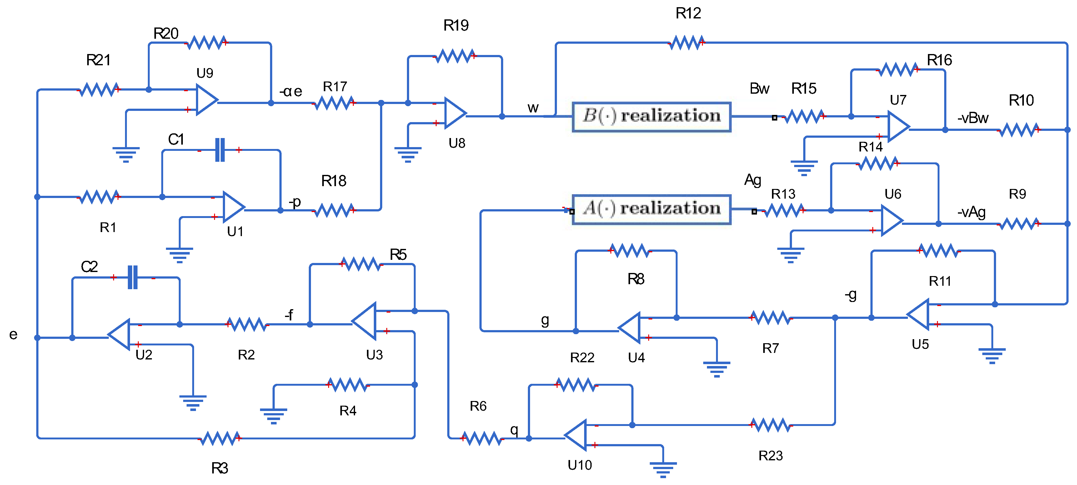
Algorithm 1 is strongly connected with the damped inertial system (42). Indeed, Algorithm 1 comes naturally into play by performing an implicit discretization of the inertial system with respect to the time variable t. Without ambiguity, we omit to write the variable t to get simplified notations. In so doing, p stands for $p\left(t\right)$, and so on. By setting $S:=Id$ and $k=1-\delta \eta$, the circuit architecture diagram of the model (42) is shown in Figure 1.

The operational amplifiers $U1,U2$ are combined with capacitors $C1,C2$, resistors $R1,R2$ to work as integrators to realize the transformations between $p,\dot{p},\ddot{p}$. The amplifier $U9$ cooperated with resistors $R20,R21$ brings about effectiveness in amplification and opposition. Hence $\dot{p}$ is translated into $-\alpha \dot{p}$. The amplifier $U3$ and resistors $R3,R4,R5,R6$ are united as the subtractor block to achieve $-\ddot{p}$. Also, in the same way, the amplifier $U8$ and resistors $R17,R18,R19$ are united as another subtractor block to achieve $p+\alpha \dot{p}$. One sees that $A((\dot{p}+\ddot{p})/k)$ and $B(p+\alpha \dot{p})$ are obtained, respectively, by “$A(·)$ realization” block and “$B(·)$ realization” block. The amplifier $U6$ cooperated with resistors $R13,R14$ brings about effectiveness in amplification and opposition, therefore, $A((\dot{p}+\ddot{p})/k)$ is translated into $-vA((\dot{p}+\ddot{p})/k)$. The amplifier $U7$ cooperated with resistors $R15,R16$ brings about effectiveness in amplification and opposition, and hence $B(p+\alpha \dot{p})$ is translated into $-vB(p+\alpha \dot{p})$. The amplifier $U5$ and resistors $R9,R10,R11,R12$ are united as the subtractor block to achieve $vA\left((\dot{p}+\ddot{p})/k\right)+vB(p+\alpha \dot{p})-(p+\alpha \dot{p})$, that is $-(\dot{p}+\ddot{p})/k$. On the other hand, $-(\dot{p}+\ddot{p})/k$ is translated into $(\dot{p}+\ddot{p})/k$ through the phase inverter composed by the operational amplifier $U4$ and resistors $R7,R8$.

4. Numerical Experiment

In this section, we consider a computational experiment to illustrate the convergence properties of the proposed method. The experiment is performed on a PC with Intel (R) Core (TM) i5-8250U CPU @1.60GHz under the MATLAB computing environment.

Digital signal reconstruction is one of the earliest and most classical problem in the file restoration, the video and image coding, the medical, the astronomical imaging and some other applications. Many problems in signal processing can be formulated as inverting the linear system, which are modeled as

$$b=Qx+\nu ,$$

(43)

where $x\in R^i$ is the original signal to be reconstructed, $\nu \in R^j$ is the noise, $b\in R^j$ is the noisy measurement, $Q\in R^{j\times i}$ is a bounded linear observation operator, often ill conditioned because it models a process with loss of information.

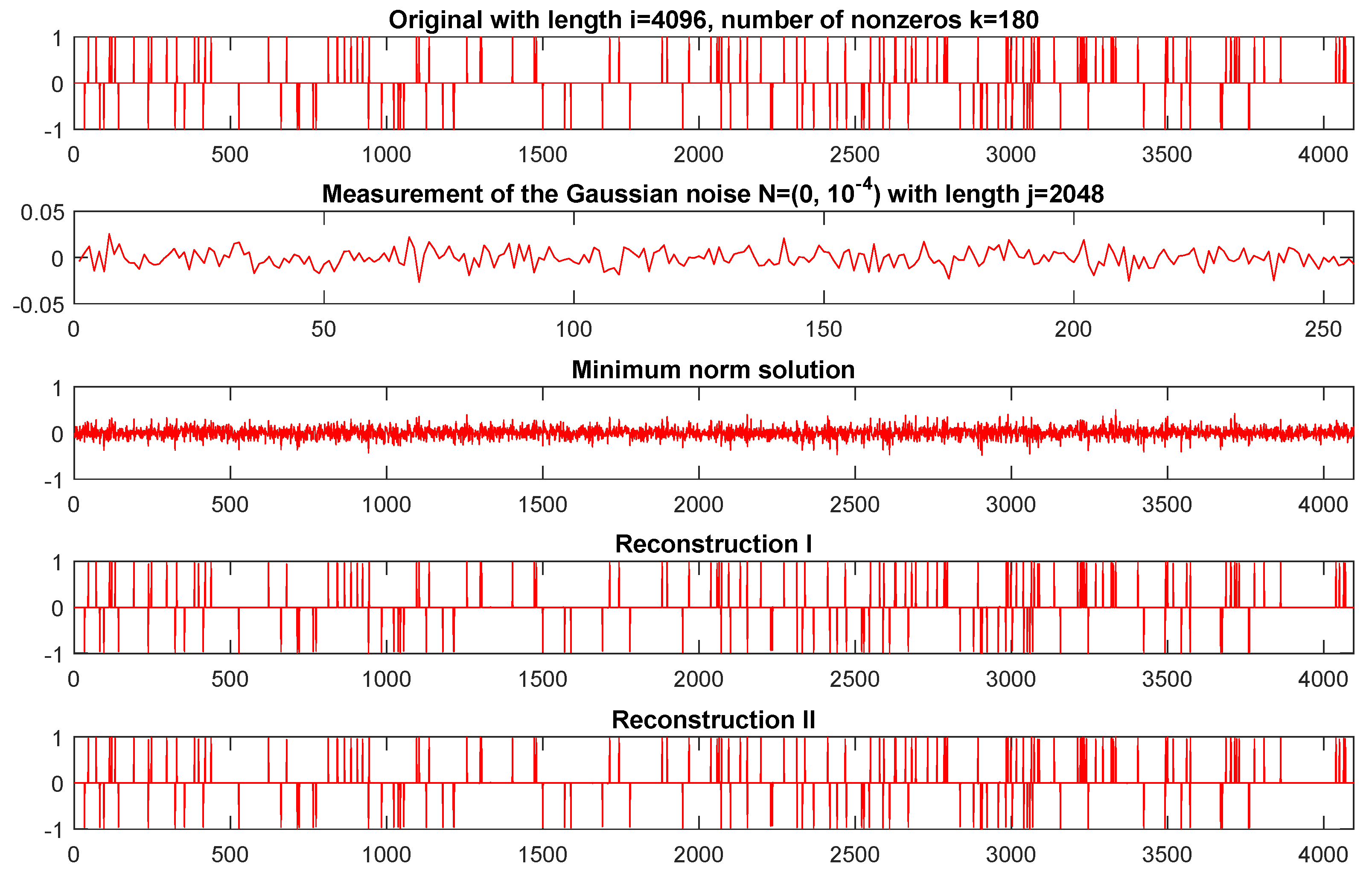
In our experiment, we consider a general compressed sensing scenario, where the goal is to reconstruct an i-length sparse signal x with exactly k nonzero components from j$(k\ll j<i)$ observations, i.e., the number of measurements is much larger than the sparsity level of x and at the same time smaller than the number of the signal length. Considering the storage limitation of the PC, we test a small size signal with $i=2^{12}$ and the original signal contains $k=180$ randomly nonzero elements. We reconstruct this signal from $j=2^{10}$ observations. More precisely, the observation $b=Qx+\nu$, where $Q\in R^{j\times i}$ is the Gaussian matrix whose elements are randomly obtained from the standard normal distribution $\mathbb{N}(0,1)$ and $\nu$ is the Gaussian noise distributed as $\mathbb{N}(0,{\sigma }^{2}I)$ with ${\sigma }^2={10}^{-4}$.

A classical and significant approach to the problems of the signal processing is the regularization method, which has attracted a considerable amount of attention and revived much interest in the compressed sensing literature. We restrict our attention to the $l_1$-regularized least squares model (43). Lasso framework is a particular instant of the linear problems of type (43) with the non-smooth $l_1$-norm as a regularizer, in which minimizes a squared loss function, and seeks to find the sparse solutions of

$${\mathrm{minimize}}_{x\in {\mathbb{R}}^i}\left\{\frac{1}{2}{\parallel Qx-b\parallel }_2^2+\alpha {\parallel x\parallel }_1\right\},$$

(44)

where the regularization parameter $\alpha (\alpha \ge 0)$ provides a tradeoff between the noise sensitivity and the fidelity to the measurements. One knows that Problem (44) always has a solution. However, it needs not to be unique. Please note that the optimal solution tends to zero as $\alpha \to \infty$. As $\alpha \to 0$, the limiting point has the minimum $l_1$ norm among all points that satisfy $Q^T(Qx-b)=0$, i.e., $x=arg{min}_{Q^T(Qx-b)=0}{\parallel x\parallel }_1$. Since the objective function of Problem (44) is convex but not differentiable, one uses a first-order optimality condition based on the subdifferential calculus. For $m=1,2,\cdots$, one can obtain the necessary and sufficient condition for the optimal solution as follows

$${\left(Q^T(Qx-b)\right)}_m\in \left\{\begin{array}{cc}\{-\alpha \},\hfill & x_m>0;\hfill \\ \left\{\alpha \right\},\hfill & x_m<0;\hfill \\ \left[-\alpha ,\alpha \right],\hfill & x_m=0.\hfill \end{array}\right.$$

From above, one sees that the optimal solution of Problem (44) is 0, for ${\left(Q^{T}b\right)}_m\in [-\alpha ,\alpha ]$, ($m=1,2,\cdots$), i.e., $\alpha \ge \parallel Q^T{b\parallel }_{\infty }$. Thus, one can now derive the formula ${\alpha }_{max}={\parallel Q^{T}b\parallel }_{\infty }.$ For $l_1$-regularized least squares; however, the convergence occurs for a finite value of $\alpha (\alpha \ge {\alpha }_{max})$. To avoid the optimal sparse solution is a zero vector, in this experiment, the regularization parameter was denoted by $\alpha :=0.01{\alpha }_{max}$, where the value of ${\alpha }_{max}$ is computed by the above formula.

The proximal methods give a better modeling of the sparsity structure in the dataset. The major step in proximal methods is to find a solution of $arg{min}_x(g\left(x\right)+\frac{1}{2\alpha }{\parallel x-v\parallel }_2^2)$ with respect to the function g and the parameter $\alpha >\parallel Q^T{b\parallel }_{\infty }$. On the other hand, the proximity operator is defined as the resolvent operator of the subgradient $pro{x}_{\alpha g}={(I+\alpha \partial g)}^{-1}$. Furthermore, the proximity operator for $l_1$-norm is described as the shrinkage operator, which is defined as $pro{x}_{\alpha \parallel ·\parallel }{\left(x\right)}_m={\left(\right|·|-\alpha )}_{+}sgn\left({\left(x\right)}_m\right)$. Now one considers the deblurring Problem (43) via the definition of the iterative shrinkage algorithm. Resorting to $g\left(x\right)={\alpha \parallel x\parallel }_1$ and $f\left(x\right)=\frac{1}{2}{\parallel Qx-b\parallel }_2^2$, one can see that Problem (44) is a special instance of the problem

$$\mathrm{find}x\in H\mathrm{such}\mathrm{that}0\in (\partial g+\nabla f)x.$$

Under the class of regularized loss minimization problems, the function g is considered to be a non-smooth regularization function and the function f is viewed as a smooth loss function with gradient being $\parallel Q^{T}Q\parallel$-cocoercive. Furthermore,

$$\left\{\begin{array}{c}pro{x}_{{\nu }_{n}g}x=\mathrm{sgn}\left({\left(x\right)}_m\right){max\left\{\right|\left(x\right)}_m|-\alpha {\nu }_n,0\},\hfill \\ (Id-{\nu }_n\nabla f)x=x-{\nu }_n{Q}^T(Qx-b),\forall {\nu }_n>0.\hfill \end{array}\right.$$

One solves the deblurring problem by using the definition of the iterative shrinkage algorithm. Setting $A:=\partial g$, $B:=\nabla f$ and $S:=Id$ in Algorithm 1, one can obtain the proximal gradient type algorithm given as follows

$$\left\{\begin{array}{c}{q}_n={(Id+{\nu }_{n}A)}^{-1}(Id-{\nu }_{n}B)(p_n+{\mu }_n(p_n-p_{n-1})),\hfill \\ p_{n+1}=(Id-\delta {\eta }_{n}S)q_n,\hfill \end{array}\right.$$

where ${\left({\mu }_n\right)}_{n\in \mathbb{N}}\in {\mathbb{R}}^{+}$. Meanwhile, we set $\delta :=\frac{1}{50}$, ${\eta }_n:=\frac{1}{n}$ and ${\nu }_n=\nu :={10}^{-8}\times \parallel Q^{T}Q\parallel$, where $n\in \mathbb{N}$. Next, we randomly choose the starting signal in the range of ${(0,1)}^{4096}$ and take the number of iterations $n=2000$ as the stopping criterion.

In this experiment, the minimum norm solution is the point in the set $\{x\in {\mathbb{R}}^{4096}|Q^{T}Qx=Q^{T}b\}$, which is closest to the original sparse signal. Thus, we can see that the result of this experiment for a signal sparse reconstruction is showed in Figure 2. By comparing the last two plots in Figure 2 and the top plot in Figure 2, one finds that the original sparse signal is recovered almost exactly. We hence conclude that our algorithm is efficient for dealing with the signal deblurring problem.

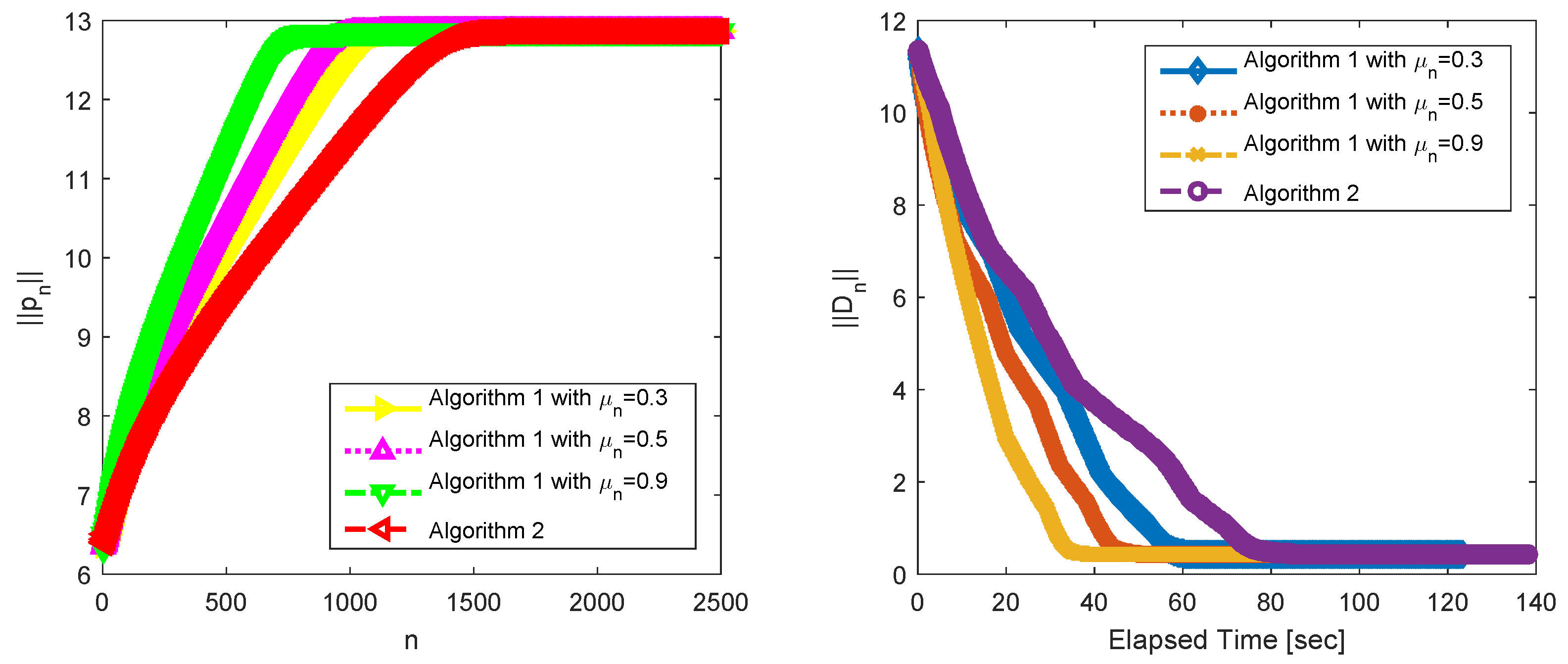
To illustrate that Algorithm 1 has a competitive performance compared with Algorithm 2, we describe the following numerical results shown in Figure 3.

The left plot in Figure 3 shows that the behaviors of the term $(\parallel p_n{\parallel )}_{n\in \mathbb{N}}$(the y-axis) with respect to the number of iterations (x-axis), where $p_n$ is generated by Algorithms 1 and 2. It can be observed from the test result reported in Figure 3 that $(\parallel p_n{\parallel )}_{n\in \mathbb{N}}$ converges to $12.8603$. Thus, we can use $(\parallel p_n{\parallel )}_{n\in \mathbb{N}}$ to study the convergence and the computational performance of Algorithms 1 and 2. We denote $D_n=p_n-x$, where x is the original signal to be reconstructed, and $p_n$ is an estimated signal of x. The right plot in Figure 3 shows that the value of $(\parallel D_n{\parallel )}_{n\in \mathbb{N}}$ (the y-axis) when the execution time in second elapses (x-axis). The sequence $(\parallel D_n{\parallel )}_{n\in \mathbb{N}}$ converges to $0.4152$ with the running time. The restoration accuracy can be measured by means of the mean squared error. We find that the mean squared error $MSE=\parallel D_n{\parallel }^2/i$ converges to $4.2088\times {10}^{-5}$, which further implies that the iterative sequence converges to the original signal x in this experiment.

We make a comparison of the behaviors of $(\parallel p_n{\parallel )}_{n\in \mathbb{N}}$, $(\parallel D_n{\parallel )}_{n\in \mathbb{N}}$ generated respectively by Algorithms 1 and 2. It shows that the bigger ${\mu }_n$ is, the fewer the required number of iterations becomes, the faster the convergence rate becomes. Furthermore, we find that all cases in Algorithm 1 need less computer time and enjoy a faster rate of the convergence than Algorithm 2. It can be observed from the plots that the changing process in all cases of Algorithm 1 outperforms Algorithm 2. The inertial extrapolation of Algorithm 1 plays a key role in the acceleration. For ${\mu }_k$ judiciously chosen, this inertial term improves the convergence speed of this algorithm.

5. Conclusions

In this paper, we introduced a variational inequality problem over the zero solution set of the inclusion problems. Since this problem has a double structure, it can be considered as a double-hierarchical optimization problem. The proposed algorithm uses the extrapolation term ${\alpha }_n(p_n-p_{n-1})$, which can be viewed as the procedure of speeding up the rate of convergence. As an application, the algorithm was used to solve the signal deblurring problem to support our convergence result.

References

- Moudafi, A. Split monotone variational inclusions. J. Optim. Theory Appl. 2011, 150, 275–283. [Google Scholar] [CrossRef]
- Iiduka, H. Two stochastic optimization algorithms for convex optimization with fixed point constraints. Optim. Methods Softw. 2019, 34, 731–757. [Google Scholar] [CrossRef] [Green Version]
- Ansari, Q.H.; Bao, T.Q. A limiting subdifferential version of Ekeland’s variational principle in set optimization. Optim. Lett. 2019, 1–5. [Google Scholar] [CrossRef]
- Al-Homidan, S.; Ansari, Q.H.; Kassay, G. Vectorial form of Ekeland variational principle with applications to vector equilibrium problems. Optimization 2020, 69, 415–436. [Google Scholar] [CrossRef]
- Li, X.; Huang, N.; Ansari, Q.H.; Yao, J.C. Convergence rate of descent method with new inexact line-search on Riemannian manifolds. J. Optim. Theory Appl. 2019, 180, 830–854. [Google Scholar] [CrossRef]
- Polyak, B.T. Some methods of speeding up the convergence of iteration methods. USSR Comput. Math. Math. Phys. 1964, 4, 1–17. [Google Scholar] [CrossRef]
- Rockafellar, R.T. Monotone operators and the proximal point algorithm. SIAM J. Control Optim. 1976, 14, 877–898. [Google Scholar] [CrossRef] [Green Version]
- Moreau, J.J. Proximité et dualité dans un espace hilbertien. Bull. De La Société Mathématique De Fr. 1965, 93, 273–299. [Google Scholar] [CrossRef]
- Bruck, R.E.; Reich, S. Nonexpansive projections and resolvents of accretive operators in Banach spaces. Houst. J. Math. 1977, 3, 459–470. [Google Scholar]
- Lions, P.L.; Mercier, B. Splitting algorithms for the sum of two nonlinear operators. SIAM J. Numer. Anal. 1979, 16, 964–979. [Google Scholar] [CrossRef]
- Cho, S.Y.; Kang, S.M. Approximation of fixed points of pseudocontraction semigroups based on a viscosity iterative process. Appl. Math. Lett. 2011, 24, 224–228. [Google Scholar] [CrossRef]
- Bot, R.I.; Csetnek, E.R. Second order forward-backward dynamical systems for monotone inclusion problems. SIAM J. Control Optim. 2016, 54, 1423–1443. [Google Scholar] [CrossRef]
- Cho, S.Y.; Kang, S.M. Approximation of common solutions of variational inequalities via strict pseudocontractions. Acta Math. Sci. 2012, 32, 1607–1618. [Google Scholar] [CrossRef]
- Cho, S.Y.; Li, W.; Kang, S.M. Convergence analysis of an iterative algorithm for monotone operators. J. Inequal. Appl. 2013, 2013, 199. [Google Scholar] [CrossRef] [Green Version]
- Luo, Y.; Shang, M.; Tan, B. A general inertial viscosity type method for nonexpansive mappings and its applications in signal processing. Mathematics 2020, 8, 288. [Google Scholar] [CrossRef] [Green Version]
- Alvarez, F.; Attouch, H. An inertial proximal method for maximal monotone operators via discretization of a nonlinear oscillator with damping. Set-Valued Anal. 2001, 9, 3–11. [Google Scholar] [CrossRef]
- Lorenz, D.A.; Pock, T. An inertial forward-backward algorithm for monotone inclusions. J. Math. Imaging Vis. 2015, 51, 311–325. [Google Scholar] [CrossRef] [Green Version]
- He, S.; Liu, L.; Xu, H.K. Optimal selections of stepsizes and blocks for the block-iterative ART. Appl. Anal. 2019, 1–14. [Google Scholar] [CrossRef]
- Cho, S.Y. Generalized mixed equilibrium and fixed point problems in a Banach space. J. Nonlinear Sci. Appl. 2016, 9, 1083–1092. [Google Scholar] [CrossRef] [Green Version]
- Liu, L. A hybrid steepest descent method for solving split feasibility problems involving nonexpansive mappings. J. Nonlinear Convex Anal. 2019, 20, 471–488. [Google Scholar]
- Kassay, G.; Reich, S.; Sabach, S. Iterative methods for solving systems of variational inequalities in reflexive Banach spaces. SIAM J. Optim. 2011, 21, 1319–1344. [Google Scholar] [CrossRef]
- Censor, Y.; Gibali, A.; Reich, S.; Sabach, S. Common solutions to variational inequalities. Set-Valued Var. Anal. 2012, 20, 229–247. [Google Scholar] [CrossRef]
- Gibali, A.; Liu, L.W.; Tang, Y.C. Note on the modified relaxation CQ algorithm for the split feasibility problem. Optim. Lett. 2018, 12, 817–830. [Google Scholar] [CrossRef]
- Cho, S.Y. Strong convergence analysis of a hybrid algorithm for nonlinear operators in a Banach space. J. Appl. Anal. Comput. 2018, 8, 19–31. [Google Scholar]
- Yamada, I. The hybrid steepest descent method for the variational inequality problem over the intersection of fixed point sets of nonexpansive mappings. Inherently Parallel Algorithms Feasibility Optim. Their Appl. 2001, 8, 473–504. [Google Scholar]
- Attouch, H.; Maingé, P.E. Asymptotic behavior of second-order dissipative evolution equations combining potential with non-potential effects. ESAIM Control Optim. Calc. Var. 2011, 17, 836–857. [Google Scholar] [CrossRef] [Green Version]
- Iiduka, H.; Takahashi, W. Strong convergence theorems for nonexpansive mappings and inverse-strongly monotone mappings. Nonlinear Anal. 2005, 61, 341–350. [Google Scholar] [CrossRef]
- Opial, Z. Weak convergence of the sequence of successive approximations for nonexpansive mappings. Bull. Am. Math. Soc. 1967, 73, 591–597. [Google Scholar] [CrossRef] [Green Version]
- Maingé, P.E. Inertial iterative process for fixed points of certain quasi-nonexpansive mappings. Set-Valued Anal. 2007, 15, 67–79. [Google Scholar] [CrossRef]
- Maingé, P.E. The viscosity approximation process for quasi-nonexpansive mappings in Hilbert spaces. Comput. Math. Appl. 2010, 59, 74–79. [Google Scholar] [CrossRef] [Green Version]
- Peypouquet, J.; Sorin, S. Evolution equations for maximal monotone operators: Asymptotic analysis in continuous and discrete time. arXiv 2009, arXiv:0905.1270. [Google Scholar]
- He, X.; Huang, T.; Yu, J.; Li, C.; Li, C. An inertial projection neural network for solving variational inequalities. IEEE Trans. Cybern. 2016, 47, 809–814. [Google Scholar] [CrossRef] [PubMed]
Figure 1.
Circuit architecture diagram of model (42), where , , , , .
Figure 2.
From top to bottom: the original signal, the noisy measurement, the minimum norm solution, the reconstruction signals respectively by Algorithm 1 () and Algorithm 2 .
Figure 3.
The behavior of with the number of iterations (left), the behavior of with the running time (right). The number of iterations is 2000. The first CPU time to compute is about s; the second CPU time to compute is about s; the third CPU time to compute is about s; the fourth CPU time to compute is about s (from top to bottom in legend).
© 2020 by the authors. Licensee MDPI, Basel, Switzerland. This article is an open access article distributed under the terms and conditions of the Creative Commons Attribution (CC BY) license (http://creativecommons.org/licenses/by/4.0/).
Share and Cite
MDPI and ACS Style
Liu, L.; Qin, X.; Yao, J.-C. A Hybrid Forward–Backward Algorithm and Its Optimization Application. Mathematics 2020, 8, 447. https://0-doi-org.brum.beds.ac.uk/10.3390/math8030447
AMA Style
Liu L, Qin X, Yao J-C. A Hybrid Forward–Backward Algorithm and Its Optimization Application. Mathematics. 2020; 8(3):447. https://0-doi-org.brum.beds.ac.uk/10.3390/math8030447
Chicago/Turabian StyleLiu, Liya, Xiaolong Qin, and Jen-Chih Yao. 2020. "A Hybrid Forward–Backward Algorithm and Its Optimization Application" Mathematics 8, no. 3: 447. https://0-doi-org.brum.beds.ac.uk/10.3390/math8030447
Note that from the first issue of 2016, this journal uses article numbers instead of page numbers. See further details here.