Power Aggregation Operators and VIKOR Methods for Complex q-Rung Orthopair Fuzzy Sets and Their Applications

Abstract

The aim of this paper is to present the novel concept of Complex q-rung orthopair fuzzy set (Cq-ROFS) which is a useful tool to cope with unresolved and complicated information. It is characterized by a complex-valued membership grade and a complex-valued non-membership grade, the distinction of which is that the sum of q-powers of the real parts (imaginary parts) of the membership and non-membership grades is less than or equal to one. To explore the study, we present some basic operational laws, score and accuracy functions and investigate their properties. Further, to aggregate the given information of Cq-ROFS, we present several weighted averaging and geometric power aggregation operators named as complex q-rung orthopair fuzzy (Cq-ROF) power averaging operator, Cq-ROF power geometric operator, Cq-ROF power weighted averaging operator, Cq-ROF power weighted geometric operator, Cq-ROF hybrid averaging operator and Cq-ROF power hybrid geometric operator. Properties and special cases of the proposed approaches are discussed in detail. Moreover, the VIKOR (“VIseKriterijumska Optimizacija I Kompromisno Resenje”) method for Cq-ROFSs is introduced and its aspects discussed. Furthermore, the above mentioned approaches apply to multi-attribute decision-making problems and VIKOR methods, in which experts state their preferences in the Cq-ROF environment to demonstrate the feasibility, reliability and effectiveness of the proposed approaches. Finally, the proposed approach is compared with existing methods through numerical examples.

1. Introduction

Multiple attribute decision making (MADM) is one of the important branches of decision science for which the principle goal is to find the best alternatives under the set of the different attributes. In it, each alternative is accessed by an expert or group of experts under the different attributes and their ratings are expressed either as a crisp number or as a linguistic number. However, in today’s challenging world, it is very common that the uncertainty plays a vital role in almost every decision-making process. Thus there is a need to handle the uncertainties in the analysis. To address this, Zadeh [1] stated the theory of fuzzy set (FS) by defining the membership degree to each element. After their appearance, several researchers have extended their theory to its more generalized ones namely, intuitionistic fuzzy set (IFS) [2], interval-valued IFS (IVIFS) [3], linguistic IVIFS [4], cubic IFS [5], Pythagorean fuzzy set (PFS) [6,7], q-rung orthopair fuzzy set [8,9]. In the existing IFS, each element is rated by an expert in terms of membership degree $\mathit{\mu }$ and non-membership degree $\mathit{\eta }$ such that $\mathit{\mu }, \mathit{\eta }\in \left[\mathbf{0},\mathbf{1}\right]; \mathit{\mu }+\mathit{\eta }\le \mathbf{1}$, while in PFS, these conditions are extended over the unit circle as $\mathit{\mu }, \mathit{\eta }\in \left[\mathbf{0},\mathbf{1}\right]; {\mathit{\mu }}^{\mathbf{2}}+{\mathit{\eta }}^{\mathbf{2}}\le \mathbf{1}$. Since their existence, several researchers have presented the different kinds of algorithms for solving the MADM problems by using aggregation operators (AOs), similarity or distance measures, hybrid operators and so forth. The several existing approaches under the IFS or PFS environments are classified into three aspects as below:

(1)

Approaches based on operators: Under it, several AOs are defined by the researchers to aggregate the intuitionistic fuzzy numbers (IFNs) and Pythagorean fuzzy numbers (PFNs). For instance, Xu and Yager [10] defined the geometric operators while Garg [11,12] defined the interactive AOs based on the hesitance degree for the pairs of intuitionistic fuzzy numbers (IFNs). He et al. [13] presented some interactive geometric AOs. In terms of PFSs, Yager [7] defined the weighted averaging AOs for Pythagorean fuzzy numbers (PFNs). Garg [14,15] extended their AOs with Einstein t-norm operations and hence presented some generalized AOs to solve the MADM problems. Zhang [16] presented ordered weighted while Zeng et al. [17] defined the hybrid AOs for PFSs. Garg [18] presented neutrality aggregation operators for PFNs to solve the MADM problems.

(2)

Approaches based on measures: The information measure such as similarity or distance measures, correlation coefficients and so forth also play a vital role in the process of MADM problems. In the IFS environment, Li and Cheng [19] defined the similarity measures for IFNs. Garg and Kumar [20] defined the similarity measures for IFNs by using connection numbers of IFNs. Ye [21] defined the cosine similarity measures for IFNs. However, under the PFS environment, Peng and Yang [22] defined the subtraction and division operations between the two or more PFNs. Yager and Abbasov [23] studied the relationship between the Pythagorean and complex numbers. Peng [24] defined some new operations between the PFSs. Wei and Wei [25] defined the similarity measure for PFS to solve the decision-making problems. Garg [26] defined the correlation coefficient between the pairs of PFNs to solve the MADM problems.

(3)

Approaches based on hybrid operators: Some researchers have utilized the extended operators to solve the MADM or MADM problems such as applications of the problems by using TOPSIS (“Technique for Order Preference with respect to the Similarity to the Ideal Solution”) [27], Bonferroni mean [28], Maclaurin symmetric mean [29] and so forth. However, for PFSs, Nie et al. [30] presented partitioned Bonferroni mean AOs to solve the DMPs with Shapley fuzzy measure. Wei and Lu [31] presented a power AOs for PFS to solve MADM problems. Gao [32] presented Hamacher Prioritized weighted AOs for PFNs. Apart from them, some interactive AOs for PFNs have been proposed by researchers in References [33,34,35].

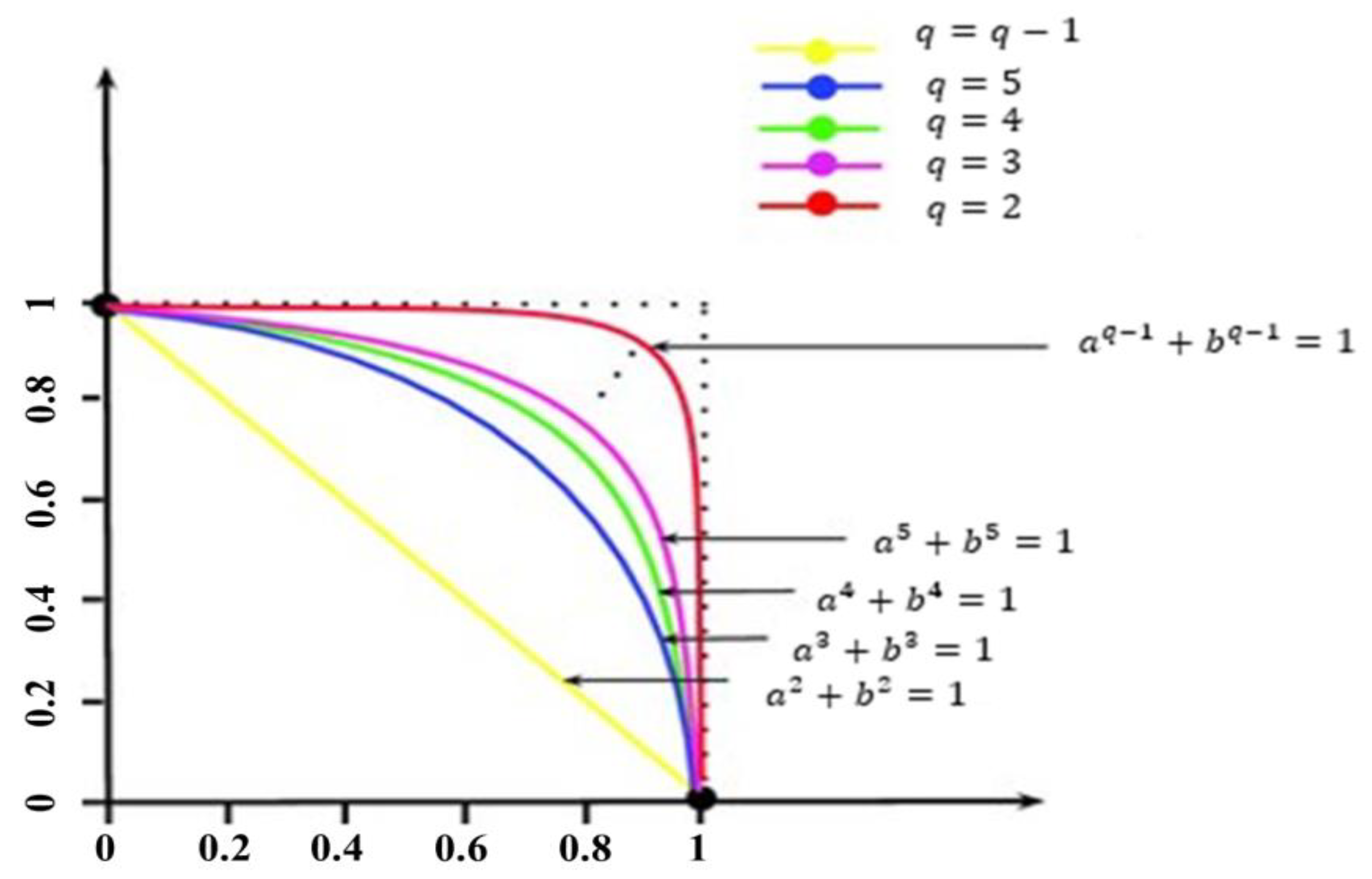
From the above extensive literature, it has been noted that IFS and PFS are widely applied in various decision making problems. However, it is observed that their approaches are limited in nature. For example, when an expert provides their information in terms of membership degree as 0.8 and non-membership degree as 0.7 then it is clearly seen that neither $\mathit{\mu }+\mathit{\eta }\le \mathbf{1}$ nor ${\mathit{\mu }}^{\mathbf{2}}+{\mathit{\eta }}^2\le \mathbf{1}$ holds. Hence, IFSs and PFSs cannot describe the information effectively. To manage such a situation, a concept of q-ROFS was introduced by Yager [9] in which each element is characterized as a membership degree $\mathit{\mu }, \mathit{\eta }$ such that $\mathit{\mu }, \mathit{\eta }\in \left[\mathbf{0},\mathbf{1}\right]; {\mathit{\mu }}^{\mathit{q}}+{\mathit{\eta }}^{\mathit{q}}\le \mathbf{1}$, with $\mathit{q}\ge 1$ interger. The q-ROFS is more effective and more general than the existing methods for handling uncertain and unpredictable information in real-decision problems with an independent degree parameter $q$. Clearly, when $q=1$ and $q=2$, the q-ROFS reduces to IFS and PFS respectively. Thus, the IFS and PFS are the special cases of the q-ROFS. The geometrical interpretation of q-ROFS is shown in Figure 1. Under the q-ROFS environment, scholars have utilized it to solve the MADM problems. Liu and Wang [36] explored the q-rung fuzzy weighted average and geometric operators. Wei et al. [37] proposed the Heronian mean operator based on the q-ROFS to solve the MADM problems. Peng et al. [38] proposed an exponential operation and aggregation operators for the q-ROFS. Liu and Wang [39] presented the q-rung orthopair fuzzy Archimedean Bonferroni mean operators for decision-making problems. Liu and Liu [40] proposed q-rung orthopair fuzzy Bonferroni mean operators and Wei et al. [41] proposed q-rung orthopair fuzzy Maclaurin symmetric mean operators. Xing et al. [42] impersonated the point operators for q-ROFSs. Garg and Chen [43] developed the neutrality aggregation operators for q-ROFS to solve the MADM problems. Peng and Dai [44] acted the multi-parametric similarity measures and its based method to solve the MADM problem under q-ROFS environment.

With the growing technologies these days, it is perceived that the above stated and similar approaches are limited in nature and are unable to handle the information which are vary with the phase of time such as “medical diagnosis”, “biometric recognition” and so forth. To deal with this, Alkouri and Salleh [45] presented the concept of the complex IFS (CIFS) in which each element is characterized by complex-valued membership and complex-valued non-membership grades represented in polar coordinates over the unit disc. Later on, Kumar and Bajaj [46] initiated the concept of the distance measures and entropy for complex intuitionistic soft sets. Rani and Garg [47] presented the distance measures to compute the degree of separation between two CIFSs. In terms of AOs, Garg and Rani [48] and Rani and Garg [49] presented weighted and power AOs for solving the MADM problems. Alkouri and Salleh [50] defined the complex intuitionistic fuzzy relations. Recently, Garg and Rani [51] presented the generalized Bonferonni mean AOs for decision-making problems. Garg and Rani [52] presented various measures for CIFS. Ullah et al. [53] extended the concept of CIFS to a complex Pythagorean fuzzy set (CPFS). However, to study the several approaches to solve the MADM under the CIFS environment, we refer to References [54,55,56].

Considering the flexibility of the complex fuzzy sets and q-ROFS to describe the uncertain information in the data, this paper presents a new concept named thecomplex q-rung orthopair fuzzy set (Cq-ROFS). To address it completely, in this paper, we extend the concept of CIFS to Cq-ROFS by taking the advantages of q-ROFS. The properties of the stated sets are also investigated. The proposed Cq-ROFS is defined under the constraint that the sum of q-powers of the real parts (imaginary parts) of the membership and non-membership grades is less than or equal to one. Further, in contrast to the standard VIKOR strategy, we have defined the VIKOR method for solving decision-making problems. Holding all the above points in mind, the primary objectives of the work are:

(1)

To establish the concept of Cq-ROFS and its fundamental properties to handle uncertain information in the data.

(2)

To define several powers weighted AOs to aggregate the different Cq-ROFS. Several properties and their special cases are also discussed in detail.

(3)

In view of the merits of the VIKOR model in considering the compromise between group utility maximization and individual regret minimization, this paper introduced the novel VIKOR method for Cq-ROFS.

(4)

Two new MADM methods, based on power operators and VIKOR methods are presented to solve the decision making problems.

(5)

The presented approaches have been demonstrated with several numerical examples to show their superiority and advantages.

The rest of the manuscript is organized as follows: in Section 2, some basic concepts of the existing sets are reviewed. In Section 3, we present a new concept of Cq-ROFS and its fundamental properties. In Section 4, we define the various power aggregation operators for Cq-ROFS and discuss their properties. In Section 5, two new MADM methods are presented to solve the problems. In Section 6, we illuminate the stated methods with several examples and compare their methods with the existing ones. Finally, Section 7 concludes the paper.

2. Preliminaries

In this section, we review the basic concept of q-ROFSs, CIFSs and their operational laws over the universal set $\mathit{X}$.

2.1. Basic Concepts

Definition 1.

An IFS$\mathit{R}$on finite universal set $\mathit{X}$ is given by [2]:

$$\mathit{R}=\left\{\left(\mathit{x},\hspace{1em}\hspace{1em}{\mathit{\mu }}_{\mathit{R}}^{\prime }\left(\mathit{x}\right),{\mathit{\eta }}_{\mathit{R}}^{\prime }\left(\mathit{x}\right)\right):\mathit{x}\in \mathit{X}\right\}$$

(1)

where${\mathit{\mu }}_{\mathit{I}}^{\prime }\left(\mathit{x}\right)$and ${\mathit{\eta }}_{\mathit{I}}^{\prime }\left(\mathit{x}\right)$ represent the “membership degree” and “non-membership degree”, respectively, with a condition:$\mathbf{0}\le {\mathit{\mu }}_{\mathit{R}}^{\prime }\left(\mathit{x}\right)+{\mathit{\eta }}_{\mathit{R}}^{\prime }\left(\mathit{x}\right)\le \mathbf{1}$.

Definition 2.

A CIFS$\mathit{R}$on finite universal set$\mathit{X}$is given by [45]:

$$\mathit{R}=\left\{\left(\mathit{x}, {\mathit{\mu }}_{\mathit{R}}^{\prime }\left(\mathit{x}\right),{\mathit{\eta }}_{\mathit{R}}^{\prime }\left(\mathit{x}\right)\right):\mathit{x}\in \mathit{X}\right\}$$

(2)

where${\mathit{\mu }}_{\mathit{R}}^{\prime }\left(\mathit{x}\right)={\mathit{\mu }}_{\mathit{R}}\left(\mathit{x}\right){\mathit{e}}^{\mathit{i}\mathbf{2}\mathit{\pi }\left({\mathit{W}}_{{\mathit{\mu }}_{\mathit{R}}}\right)}$and${\mathit{\eta }}_{\mathit{R}}^{\prime }\left(\mathit{x}\right)={\mathit{\eta }}_{\mathit{R}}\left(\mathit{x}\right){\mathit{e}}^{\mathit{i}\mathbf{2}\mathit{\pi }\left({\mathit{W}}_{{\mathit{\eta }}_{\mathit{R}}}\right)}$, represents the complex-valued truth and complex-valued falsity degrees, with a conditions: $\mathbf{0}\le {\mathit{\mu }}_{\mathit{R}}\left(\mathit{x}\right)+{\mathit{\eta }}_{\mathit{R}}\left(\mathit{x}\right)\le \mathbf{1},\mathbf{0}\le {\mathit{W}}_{{\mathit{\mu }}_{\mathit{R}}}\left(\mathit{x}\right)+{\mathit{W}}_{{\mathit{\eta }}_{\mathit{R}}}\left(\mathit{x}\right)\le \mathbf{1}$.

Definition 3.

For a two CIFNs${\mathit{R}}_{\mathbf{1}}=\left({\mathit{\mu }}_{\mathbf{1}}\left(\mathit{x}\right){\mathit{e}}^{\mathit{i}\mathbf{2}\mathit{\pi }\left({\mathit{W}}_{{\mathit{\mu }}_{\mathbf{1}}}\right)},{\mathit{\eta }}_{\mathbf{1}}\left(\mathit{x}\right){\mathit{e}}^{\mathit{i}\mathbf{2}\mathit{\pi }\left({\mathit{W}}_{{\mathit{\eta }}_{\mathbf{1}}}\right)}\right)$and${\mathit{R}}_{\mathbf{2}}=\left({\mathit{\mu }}_{\mathbf{2}}\left(\mathit{x}\right){\mathit{e}}^{\mathit{i}\mathbf{2}\mathit{\pi }\left({\mathit{W}}_{{\mathit{\mu }}_{\mathbf{2}}}\right)},{\mathit{\eta }}_{\mathbf{2}}\left(\mathit{x}\right){\mathit{e}}^{\mathit{i}\mathbf{2}\mathit{\pi }\left({\mathit{W}}_{{\mathit{\eta }}_{\mathbf{2}}}\right)}\right)$and $\mathit{\gamma }>\mathbf{0}$ be any real number [45]. Then

(1) 

${\mathit{R}}_{\mathbf{1}}\mathbf{\oplus }{\mathit{R}}_{\mathbf{2}}=\left(\left({\mathit{\mu }}_{\mathbf{1}}+{\mathit{\mu }}_{\mathbf{2}}-{\mathit{\mu }}_{\mathbf{1}}{\mathit{\mu }}_{\mathbf{2}}\right){\mathit{e}}^{\mathit{i}\mathbf{2}\mathit{\pi }\left({\mathit{W}}_{{\mathit{\mu }}_{\mathbf{1}}}+{\mathit{W}}_{{\mathit{\mu }}_{\mathbf{2}}}-{\mathit{W}}_{{\mathit{\mu }}_{\mathbf{1}}}{\mathit{W}}_{{\mathit{\mu }}_{\mathbf{2}}}\right)},\left({\mathit{\eta }}_{\mathbf{1}}{\mathit{\eta }}_{\mathbf{2}}\right){\mathit{e}}^{\mathit{i}\mathbf{2}\mathit{\pi }\left({\mathit{W}}_{{\mathit{\eta }}_{\mathbf{1}}}{\mathit{W}}_{{\mathit{\eta }}_{\mathbf{2}}}\right)}\right)$;

(2) 

${\mathit{R}}_{\mathbf{1}}\mathbf{\otimes }{\mathit{R}}_{\mathbf{2}}=\left(\left({\mathit{\mu }}_{\mathbf{1}}{\mathit{\mu }}_{\mathbf{2}}\right){\mathit{e}}^{\mathit{i}\mathbf{2}\mathit{\pi }\left({\mathit{W}}_{{\mathit{\mu }}_{\mathbf{1}}}{\mathit{W}}_{{\mathit{\mu }}_{\mathbf{2}}}\right)},\left({\mathit{\eta }}_{\mathbf{1}}+{\mathit{\eta }}_{\mathbf{2}}-{\mathit{\eta }}_{\mathbf{1}}{\mathit{\eta }}_{\mathbf{2}}\right){\mathit{e}}^{\mathit{i}\mathbf{2}\mathit{\pi }\left({\mathit{W}}_{{\mathit{\eta }}_{\mathbf{1}}}+{\mathit{W}}_{{\mathit{\eta }}_{\mathbf{2}}}-{\mathit{W}}_{{\mathit{\eta }}_{\mathbf{1}}}{\mathit{W}}_{{\mathit{\eta }}_{\mathbf{2}}}\right)}\right)$;

(3) 

$\mathit{\gamma }{\mathit{R}}_{\mathbf{1}}=\left(\left(\mathbf{1}-{\left(\mathbf{1}-{\mathit{\mu }}_{\mathbf{1}}\right)}^{\mathit{\gamma }}\right){\mathit{e}}^{\mathit{i}\mathbf{2}\mathit{\pi }\left(\mathbf{1}-{\left(\mathbf{1}-{\mathit{W}}_{{\mathit{\mu }}_{\mathbf{1}}}\right)}^{\mathit{\gamma }}\right)},{\mathit{\eta }}_{\mathbf{1}}^{\mathit{\gamma }}{\mathit{e}}^{\mathit{i}\mathbf{2}\mathit{\pi }{\mathit{W}}_{{\mathit{\eta }}_{\mathbf{1}}}^{\mathit{\gamma }}}\right)$;

(4) 

$\mathit{\gamma }{\mathit{R}}_{\mathbf{1}}=\left({\mathit{\mu }}_{\mathbf{1}}^{\mathit{\gamma }}{\mathit{e}}^{\mathit{i}\mathbf{2}\mathit{\pi }{\mathit{W}}_{{\mathit{\mu }}_{\mathbf{1}}}^{\mathit{\gamma }}},\left(\mathbf{1}-{\left(\mathbf{1}-{\mathit{\eta }}_{\mathbf{1}}\right)}^{\mathit{\gamma }}\right){\mathit{e}}^{\mathit{i}\mathbf{2}\mathit{\pi }\left(\mathbf{1}-{\left(\mathbf{1}-{\mathit{W}}_{{\mathit{\eta }}_{\mathbf{1}}}\right)}^{\mathit{\gamma }}\right)}\right)$.

Definition 4.

A PFS$\mathit{R}$on finite universal set $\mathit{X}$ is given by [7]:

$$\mathit{R}=\left\{\left(\mathit{x}, {\mathit{\mu }}_{\mathit{R}}^{\prime }\left(\mathit{x}\right),{\mathit{\eta }}_{\mathit{R}}^{\prime }\left(\mathit{x}\right)\right):\mathit{x}\in \mathit{X}\right\}$$

(3)

with a condition: $\mathbf{0}\le {\mathit{\mu }}_{\mathit{R}}^{\prime }{}^{\mathbf{2}}\left(\mathit{x}\right)+{\mathit{\eta }}_{\mathit{R}}^{\prime }{}^{\mathbf{2}}\left(\mathit{x}\right)\le \mathbf{1}$, where${\mathit{\mu }}_{\mathit{R}}^{\prime },{\mathit{\eta }}_{\mathit{R}}^{\prime }:\mathit{X}\to \left[\mathbf{0},\mathbf{1}\right]$.

Definition 5.

A CPFS$\mathit{R}$on finite universal set $\mathit{X}$ is given by [53]:

$$\mathit{R}=\left\{\left(\mathit{x},\hspace{1em}\hspace{1em}{\mathit{\mu }}_{\mathit{R}}^{\prime }\left(\mathit{x}\right),{\mathit{\eta }}_{\mathit{R}}^{\prime }\left(\mathit{x}\right)\right):\mathit{x}\in \mathit{X}\right\}$$

(4)

where${\mathit{\mu }}_{\mathit{R}}^{\prime }\left(\mathit{x}\right)={\mathit{\mu }}_{\mathit{R}}\left(\mathit{x}\right){\mathit{e}}^{\mathit{i}\mathbf{2}\mathit{\pi }\left({\mathit{W}}_{{\mathit{\mu }}_{\mathit{R}}}\right)}$and${\mathit{\eta }}_{\mathit{R}}^{\prime }\left(\mathit{x}\right)={\mathit{\eta }}_{\mathit{R}}\left(\mathit{x}\right){\mathit{e}}^{\mathit{i}\mathbf{2}\mathit{\pi }\left({\mathit{W}}_{{\mathit{\eta }}_{\mathit{R}}}\right)}$, represents the complex-valued truth and complex-valued falsity degrees, with a conditions: $\mathbf{0}\le {\mathit{\mu }}_{\mathit{R}}^{\mathbf{2}}\left(\mathit{x}\right)+{\mathit{\eta }}_{\mathit{R}}^{\mathbf{2}}\left(\mathit{x}\right)\le \mathbf{1},\mathbf{0}\le {\mathit{W}}_{{\mathit{\mu }}_{\mathit{R}}}^{\mathbf{2}}\left(\mathit{x}\right)+{\mathit{W}}_{{\eta }_{\mathit{R}}}^{\mathbf{2}}\left(\mathit{x}\right)\le \mathbf{1}$, where${\mathit{\mu }}_{\mathit{R}},{\mathit{W}}_{{\mathit{\mu }}_{\mathit{R}}},{\mathit{\eta }}_{\mathit{R}},{\mathit{W}}_{{\mathit{\eta }}_{\mathit{R}}}\in \left[\mathbf{0},\mathbf{1}\right]$.

Definition 6.

For a two CPFNs${\mathit{R}}_{\mathbf{1}}=\left({\mathit{\mu }}_{\mathbf{1}}\left(\mathit{x}\right){\mathit{e}}^{\mathit{i}\mathbf{2}\mathit{\pi }\left({\mathit{W}}_{{\mathit{\mu }}_{\mathbf{1}}}\right)},{\mathit{\eta }}_{\mathbf{1}}\left(\mathit{x}\right){\mathit{e}}^{\mathit{i}\mathbf{2}\mathit{\pi }\left({\mathit{W}}_{{\mathit{\eta }}_{\mathbf{1}}}\right)}\right)$and${\mathit{R}}_{\mathbf{2}}=\left({\mathit{\mu }}_{\mathbf{2}}\left(\mathit{x}\right){\mathit{e}}^{\mathit{i}\mathbf{2}\mathit{\pi }\left({\mathit{W}}_{{\mathit{\mu }}_{\mathbf{2}}}\right)},{\mathit{\eta }}_{\mathbf{2}}\left(\mathit{x}\right){\mathit{e}}^{\mathit{i}\mathbf{2}\mathit{\pi }\left({\mathit{W}}_{{\mathit{\eta }}_{\mathbf{2}}}\right)}\right)$and $\mathit{\gamma }>\mathbf{0}$ be any real number [53]. Then

(1) 

${\mathit{R}}_{\mathbf{1}}\mathbf{\oplus }{\mathit{R}}_{\mathbf{2}}=\left({\left({\mathit{\mu }}_{\mathbf{1}}^{\mathbf{2}}+{\mathit{\mu }}_{\mathbf{2}}^{\mathbf{2}}-{\mathit{\mu }}_{\mathbf{1}}^{\mathbf{2}}{\mathit{\mu }}_{\mathbf{2}}^{\mathbf{2}}\right)}^{\frac{\mathbf{1}}{\mathbf{2}}}{\mathit{e}}^{\mathit{i}\mathbf{2}\mathit{\pi }{\left({\mathit{W}}_{{\mathit{\mu }}_{\mathbf{1}}}^{\mathbf{2}}+{\mathit{W}}_{{\mathit{\mu }}_{\mathbf{2}}}^{\mathbf{2}}-{\mathit{W}}_{{\mathit{\mu }}_{\mathbf{1}}}^{\mathbf{2}}{\mathit{W}}_{{\mathit{\mu }}_{\mathbf{2}}}^{\mathbf{2}}\right)}^{\frac{\mathbf{1}}{\mathbf{2}}}},\left({\mathit{\eta }}_{\mathbf{1}}{\mathit{\eta }}_{\mathbf{2}}\right){\mathit{e}}^{\mathit{i}\mathbf{2}\mathit{\pi }\left({\mathit{W}}_{{\mathit{\eta }}_{\mathbf{1}}}{\mathit{W}}_{{\mathit{\eta }}_{\mathbf{2}}}\right)}\right)$;

(2) 

${\mathit{R}}_{\mathbf{1}}\mathbf{\otimes }{\mathit{R}}_{\mathbf{2}}=\left(\left({\mathit{\mu }}_{\mathbf{1}}{\mathit{\mu }}_{\mathbf{2}}\right){\mathit{e}}^{\mathit{i}\mathbf{2}\mathit{\pi }\left({\mathit{W}}_{{\mathit{\mu }}_{\mathbf{1}}}{\mathit{W}}_{{\mathit{\mu }}_{\mathbf{2}}}\right)},{\left({\mathit{\eta }}_{\mathbf{1}}^{\mathbf{2}}+{\mathit{\eta }}_{\mathbf{2}}^{\mathbf{2}}-{\mathit{\eta }}_{\mathbf{1}}^{\mathbf{2}}{\mathit{\eta }}_{\mathbf{2}}^{\mathbf{2}}\right)}^{\frac{\mathbf{1}}{\mathbf{2}}}{\mathit{e}}^{\mathit{i}\mathbf{2}\mathit{\pi }{\left({\mathit{W}}_{{\mathit{\eta }}_{\mathbf{1}}}^{\mathbf{2}}+{\mathit{W}}_{{\mathit{\eta }}_{\mathbf{2}}}^{\mathbf{2}}-{\mathit{W}}_{{\mathit{\eta }}_{\mathbf{1}}}^{\mathbf{2}}{\mathit{W}}_{{\mathit{\eta }}_{\mathbf{2}}}^{\mathbf{2}}\right)}^{\frac{\mathbf{1}}{\mathbf{2}}}}\right)$;

(3) 

$\mathit{\gamma }{\mathit{R}}_{\mathbf{1}}=\left({\left(\mathbf{1}-{\left(\mathbf{1}-{\mathit{\mu }}_{\mathbf{1}}^{\mathbf{2}}\right)}^{\mathit{\gamma }}\right)}^{\frac{\mathbf{1}}{\mathbf{2}}}{\mathit{e}}^{\mathit{i}\mathbf{2}\mathit{\pi }{\left(\mathbf{1}-{\left(\mathbf{1}-{\mathit{W}}_{{\mathit{\mu }}_{\mathbf{1}}}^{\mathbf{2}}\right)}^{\mathit{\gamma }}\right)}^{\frac{\mathbf{1}}{\mathbf{2}}}},{\mathit{\eta }}_{\mathbf{1}}^{\mathit{\gamma }}{\mathit{e}}^{\mathit{i}\mathbf{2}\mathit{\pi }{\mathit{W}}_{{\mathit{\eta }}_{\mathbf{1}}}^{\mathit{\gamma }}}\right)$;

(4) 

$\mathit{\gamma }{\mathit{R}}_{\mathbf{1}}=\left({\mathit{\mu }}_{\mathbf{1}}^{\mathit{\gamma }}{\mathit{e}}^{\mathit{i}\mathbf{2}\mathit{\pi }{\mathit{W}}_{{\mathit{\mu }}_{\mathbf{1}}}^{\mathit{\gamma }}},{\left(\mathbf{1}-{\left(\mathbf{1}-{\mathit{\eta }}_{\mathbf{1}}^{\mathbf{2}}\right)}^{\mathit{\gamma }}\right)}^{\frac{\mathbf{1}}{\mathbf{2}}}{\mathit{e}}^{\mathit{i}\mathbf{2}\mathit{\pi }{\left(\mathbf{1}-{\left(\mathbf{1}-{\mathit{W}}_{{\mathit{\eta }}_{\mathbf{1}}}^{\mathbf{2}}\right)}^{\mathit{\gamma }}\right)}^{\frac{\mathbf{1}}{\mathbf{2}}}}\right)$.

Definition 7.

A q-ROFS$\mathit{R}$on finite universal set $\mathit{X}$ is given by [9]:

$$\mathit{R}=\left\{\left(\mathit{x}, {\mathit{\mu }}_{\mathit{R}}^{\prime }\left(\mathit{x}\right),{\mathit{\eta }}_{\mathit{R}}^{\prime }\left(\mathit{x}\right)\right):\mathit{x}\in \mathit{X}\right\}$$

(5)

with a condition:$\mathbf{0}\le {\mathit{\mu }}_{\mathit{R}}^{\prime }{}^{\mathit{q}}\left(\mathit{x}\right)+{\mathit{\eta }}_{\mathit{R}}^{\prime }{}^{\mathit{q}}\left(\mathit{x}\right)\le \mathbf{1}$. The hesitancy degree is denoted and defined by${\mathit{\theta }}_{\mathit{R}}={\left(\mathbf{1}-{\mathit{\mu }}_{\mathit{R}}^{\prime }{}^{\mathit{q}}\left(\mathit{x}\right)-{\mathit{\eta }}_{\mathit{R}}^{\prime }{}^{\mathit{q}}\left(\mathit{x}\right)\right)}^{\frac{\mathbf{1}}{\mathit{q}}}$. The q-rung orthopair fuzzy number is given by$\mathit{R}=\left({\mathit{\mu }}_{\mathit{R}}^{\prime }\left(\mathit{x}\right),{\mathit{\eta }}_{\mathit{R}}^{\prime }\left(\mathit{x}\right)\right)$.

Definition 8.

A family of data${\mathit{R}}_{\mathit{i}}\left(\mathit{i}=\mathbf{1},\mathbf{2},\dots ,\mathit{n}\right)$, then the power averaging operator is given by [57]:

$$\mathit{P}\mathit{A}\left({\mathit{R}}_{\mathbf{1}},{\mathit{R}}_{\mathbf{2}},\dots ,{\mathit{R}}_{\mathit{n}}\right)=\frac{{{\displaystyle \mathbf{\sum }}}_{\mathit{j}=\mathbf{1}}^{\mathit{n}}\left(\left(\mathbf{1}+\mathrm{Ṱ}\left({\mathit{R}}_{\mathit{j}}\right)\right){\mathit{R}}_{\mathit{j}}\right)}{{{\displaystyle \mathbf{\sum }}}_{\mathit{j}=\mathbf{1}}^{\mathit{n}}\left(\mathbf{1}+\mathrm{Ṱ}\left({\mathit{R}}_{\mathit{j}}\right)\right)}$$

where${{\displaystyle \mathbf{\sum }}}_{\begin{array}{c}\mathit{i}=\mathbf{1}\\ \mathit{i}\ne \mathit{j}\end{array}}^{\mathit{n}}\mathbf{sup}\left({\mathit{R}}_{\mathit{i}},{\mathit{R}}_{\mathit{j}}\right)=\mathrm{Ṱ}\left({\mathit{R}}_{\mathit{i}}\right)$and$\mathbf{sup}\left({\mathit{R}}_{\mathit{i}},{\mathit{R}}_{\mathit{j}}\right)$is called support degree, which holds the axioms:$\mathbf{sup}\left({\mathit{R}}_{\mathit{i}},{\mathit{R}}_{\mathit{j}}\right)\in \left[\mathbf{0},\mathbf{1}\right]$; $\mathbf{sup}\left({\mathit{R}}_{\mathit{i}},{\mathit{R}}_{\mathit{j}}\right)=\mathbf{sup}\left({\mathit{R}}_{\mathit{j}},{\mathit{R}}_{\mathit{i}}\right)$; and$\mathbf{sup}\left({\mathit{R}}_{\mathit{i}},{\mathit{R}}_{\mathit{j}}\right)\ge \mathbf{sup}\left({\mathit{R}}_{\mathit{k}},{\mathit{R}}_{\mathit{l}}\right)\Rightarrow \left|{\mathit{R}}_{\mathit{i}}-{\mathit{R}}_{\mathit{j}}\right|\le \left|{\mathit{R}}_{\mathit{k}}-{\mathit{R}}_{\mathit{l}}\right|$.

2.2. Standard VIKOR Method

VIKOR (“VIseKriterijumska Optimizacija I Kompromisno Resenje”) [58] is a standard and important method to solve the decision making problem. In the VIKOR method, alternatives are assessed by considering the compromise between group utility maximization and individual regret minimization. The standard procedure for solving the decision making problems with the VIKOR method is summarized below:

Consider $m$ alternatives $X_1,X_2,\dots ,X_m$ and $n$ attributes ${\mathrm{Ẫ}}_1,{\mathrm{Ẫ}}_2,\dots ,{\mathrm{Ẫ}}_n$ with respect to weight vectors such that $w={\left(w_1,w_2,\dots ,w_n\right)}^{\mathrm{Ṱ}}, {\sum }_{j=1}^n{w}_j=1$ and the compromise ranking by VIKOR methods starts with the form of $L_p$-metric [59].

$$L_{pi}={\left\{{\displaystyle \sum }_{j=1}^n{\left[\left(\frac{R_j^{*}-R_{ij}}{R_j^{*}-R_j^{-}}\right)\right]}^p\right\}}^{\frac{1}{p}},1\le p\le \infty ,i=1,2,\dots ,m$$

In the VIKOR method, the maximum group utility can be gotten by $\min S_i$ and minimum individual regret can be gotten by $min S_i^{\prime }$, where $S_i=L_{1,i}$ and $S_i^{\prime }=L_{\infty ,i}$. The various steps involved in the VIKOR method are summarized as follows:

Step 1: Computing the virtual positive ideal $x_j^{*}$ and the virtual negative ideal $x_j^{-}$ values under the attributes ${\mathrm{Ẫ}}_j$, we have

$$x_j^{*}=ma{x}_i\left(x_{ij}\right),x_j^{-}=mi{n}_i\left(x_{ij}\right)$$

Step 2: Computing the values of group utility $S_i$ and $S_i^{\prime }$, we have

$$S_i=\frac{{\sum }_{j=1}^n{w}_j\parallel R_j^{*}-R_{ij}\parallel }{\parallel R_j^{*}-R_j^{-}\parallel }\mathrm{and}{S}_i^{\prime }=\frac{ma{x}_j{w}_j\parallel R_j^{*}-R_{ij}\parallel }{\parallel R_j^{*}-R_j^{-}\parallel }$$

Step 3: Computing the values of $Q_i,i=1,2,\dots ,m$, we have

$$Q_i=\frac{v\left(S_i-S^{*}\right)}{\left(S^{-}-S^{*}\right)}+\frac{\left(1-v\right)\left(S_i^{\prime }-{S^{\prime }}^{*}\right)}{\left({S^{\prime }}^{-}-{S^{\prime }}^{*}\right)},$$

where $S^{*}=mi{n}_i\left(S_i\right),S^{-}=ma{x}_i\left(S_i\right),{S^{\prime }}^{*}=mi{n}_i\left(S_i^{\prime }\right)$ and ${S^{\prime }}^{-}=ma{x}_i\left(S_i^{\prime }\right)$, the symbol $v$ is the balance parameter which can balance the group of utility and individual regret.

Step 4: Using the values of $S,S^{\prime }$ and $Q$ and ranking the alternatives, then we will obtain the compromise solution.

Step 5: When we get the compromise solution $X^{\left(1\right)}$ in steps 4, then it satisfied the following two conditions.

• Condition 1:Acceptable advantages: $Q\left(X^{\left(2\right)}\right)-Q\left(X^{\left(1\right)}\right)\ge \frac{1}{m-1}$, where $Q\left(X^{\left(2\right)}\right)$ is the $Q$ value in the second position of all ranking alternatives produced by the value of $Q$ and $m$ number of alternatives.
• Condition 2:Acceptable stability: Alternative $X^{\left(1\right)}$ must also in the first position of all ranking alternatives produced by the values of $S$ or $S^{\prime }$.

If one of the above conditions is not met, then we collected the compromise alternatives and not one compromise solution. If condition 2 does not hold, then we will examine the alternatives $X^{\left(1\right)}$ and $X^{\left(2\right)}$ should be the compromise solution. If condition 2 does not hold, then the maximum $M$ eximane by the formula $Q\left(X^{\left(M\right)}\right)-Q\left(X^{\left(1\right)}\right)<MQ=\frac{1}{m-1}$, we examined the alternatives $X^{\left(1\right)},X^{\left(2\right)},\dots ,X^{\left(m\right)}$ are the compromise solution.

3. Proposed Cq-ROFS

In this section, we present the new concept of Complex q-rung orthopair fuzzy set (Cq-ROFS) and state their properties.

Definition 9.

A Cq-ROFS$R$on finite universal set $\mathit{X}$ is given by:

$$R=\left\{\left(x, {\mu }_R^{\prime }\left(x\right),{\eta }_R^{\prime }\left(x\right)\right):x\in X\right\},$$

(6)

where${\mu }_R^{\prime }\left(x\right)={\mu }_R\left(x\right)e^{i2\pi \left(W_{{\mu }_R}\right)}$and${\eta }_R^{\prime }\left(x\right)={\eta }_R\left(x\right)e^{i2\pi \left(W_{{\eta }_R}\right)}$, represents the complex-valued truth and complex-valued falsity degrees, with a conditions: $0\le {\mu }_R^q\left(x\right)+{\eta }_R^q\left(x\right)\le 1,0\le W_{{\mu }_R}^q\left(x\right)+W_{{\eta }_R}^q\left(x\right)\le 1$. The complex q-rung orthopair fuzzy number (Cq-ROFN) is denoted by:$R=\left({\mu }_R\left(x\right)e^{i2\pi \left(W_{{\mu }_R}\right)},{\eta }_R\left(x\right)e^{i2\pi \left(W_{{\eta }_R}\right)}\right)$.

Remark 1.

The hesitancy degree is denoted and defined by${\mathit{\theta }}_{\mathit{R}}={\left(\mathbf{1}-{\mathit{\mu }}_{\mathit{R}}^{\mathit{q}}\left(\mathit{x}\right)-{\mathit{\eta }}_{\mathit{R}}^{\mathit{q}}\left(\mathit{x}\right)\right)}^{\frac{\mathbf{1}}{\mathit{q}}}{\mathit{e}}^{\mathit{i}\mathbf{2}\mathit{\pi }{\left(\mathbf{1}-{\mathit{W}}_{{\mathit{\mu }}_{\mathit{R}}}^{\mathit{q}}\left(\mathit{x}\right)-{\mathit{W}}_{{\mathit{\eta }}_{\mathit{R}}}^{\mathit{q}}\left(\mathit{x}\right)\right)}^{\frac{\mathbf{1}}{\mathit{q}}}}$.

Definition 10.

For a two Cq-ROFNs$R_1=\left({\mu }_1\left(x\right)e^{i2\pi \left(W_{{\mu }_1}\right)},{\eta }_1\left(x\right)e^{i2\pi \left(W_{{\eta }_1}\right)}\right)$and$R_2=\left({\mu }_2\left(x\right)e^{i2\pi \left(W_{{\mu }_2}\right)},{\eta }_2\left(x\right)e^{i2\pi \left(W_{{\eta }_2}\right)}\right)$, then

(1) 

$R_1\subseteq R_2$iff${\mu }_1\left(x\right)\lesssim {\mu }_2\left(x\right),{\eta }_1\left(x\right)\ge {\eta }_2\left(x\right)$and$W_{{\mu }_1}\lesssim W_{{\mu }_2},W_{{\eta }_1}\ge W_{{\eta }_2}$.

(2) 

$R_1=R_2$if${\mu }_1\left(x\right)={\mu }_2\left(x\right),{\eta }_1\left(x\right)={\eta }_2\left(x\right)$and$W_{{\mu }_1}=W_{{\mu }_2},W_{{\eta }_1}=W_{{\eta }_2}$.

(3) 

$R_1^c=\left({\eta }_1\left(x\right)e^{i2\pi \left(W_{{\eta }_1}\right)},{\mu }_1\left(x\right)e^{i2\pi \left(W_{{\mu }_1}\right)}\right)$.

To compare two or more Cq-ROFNs, we define the score and accuracy functions for them as

Definition 11.

For Cq-ROFN$R_1=\left({\mu }_1\left(x\right)e^{i2\pi \left(W_{{\mu }_1}\right)},{\eta }_1\left(x\right)e^{i2\pi \left(W_{{\eta }_1}\right)}\right)$, a score function for it is defined as

$$S\left(R_1\right)={\mu }_1^q-{\eta }_1^q+W_{{\mu }_1}^q-W_{{\eta }_1}^q$$

(7)

while an accuracy function H is stated as

$$H\left(R_1\right)={\mu }_1^q+{\eta }_1^q+W_{{\mu }_1}^q+W_{{\eta }_1}^q$$

(8)

Definition 12.

For two Cq-ROFNs$R_1$and $R_2$ and by using Definition 11, we define an order relation between them as follows

(1) 

If$S\left(R_1\right)>S\left(R_2\right)$then$R_1>R_2$, similarly if$H\left(R_1\right)>H\left(R_2\right)$then$R_1>R_2$.

(2) 

If$S\left(R_1\right)=S\left(R_2\right)$and$H\left(R_1\right)>H\left(R_2\right)$then$R_1>R_2$.

Definition 13.

For a two Cq-ROFNs$R_1=\left({\mu }_1\left(x\right)e^{i2\pi \left(W_{{\mu }_1}\right)},{\eta }_1\left(x\right)e^{i2\pi \left(W_{{\eta }_1}\right)}\right)$and$R_2=\left({\mu }_2\left(x\right)e^{i2\pi \left(W_{{\mu }_2}\right)},{\eta }_2\left(x\right)e^{i2\pi \left(W_{{\eta }_2}\right)}\right)$and $\gamma >0$ be any real number. Then

(1) 

$R_1\oplus R_2=\left({\left({\mu }_1^q+{\mu }_2^q-{\mu }_1^q{\mu }_2^q\right)}^{\frac{1}{q}}{e}^{i2\pi {\left(W_{{\mu }_1}^q+W_{{\mu }_2}^q-W_{{\mu }_1}^q{W}_{{\mu }_2}^q\right)}^{\frac{1}{q}}},\left({\eta }_1{\eta }_2\right)e^{i2\pi \left(W_{{\eta }_1}{W}_{{\eta }_2}\right)}\right)$;

(2) 

$R_1\otimes R_2=\left(\left({\mu }_1{\mu }_2\right)e^{i2\pi \left(W_{{\mu }_1}{W}_{{\mu }_2}\right)},{\left({\eta }_1^q+{\eta }_2^q-{\eta }_1^q{\eta }_2^q\right)}^{\frac{1}{q}}{e}^{i2\pi {\left(W_{{\eta }_1}^q+W_{{\eta }_2}^q-W_{{\eta }_1}^q{W}_{{\eta }_2}^q\right)}^{\frac{1}{q}}}\right)$;

(3) 

$\gamma R_1=\left({\left(1-{\left(1-{\mu }_1^q\right)}^{\gamma }\right)}^{\frac{1}{q}}{e}^{i2\pi {\left(1-{\left(1-W_{{\mu }_1}^q\right)}^{\gamma }\right)}^{\frac{1}{q}}},{\eta }_1^{\gamma }{e}^{i2\pi W_{{\eta }_1}^{\gamma }}\right)$;

(4) 

$\gamma R_1=\left({\mu }_1^{\gamma }{e}^{i2\pi W_{{\mu }_1}^{\gamma }},{\left(1-{\left(1-{\eta }_1^q\right)}^{\gamma }\right)}^{\frac{1}{q}}{e}^{i2\pi {\left(1-{\left(1-W_{{\eta }_1}^q\right)}^{\gamma }\right)}^{\frac{1}{q}}}\right)$.

Theorem 1.

For two Cq-ROFNs$R_1$and$R_2$with real number$\gamma >0$, then$R_1\oplus R_2,\gamma R_1,R_1\otimes R_2$and $R_1^{\gamma }$ as defined in Definition 13, are Cq-ROFNs.

Proof. 

For two Cq-ROFNs $R_1=\left({\mu }_1\left(x\right)e^{i2\pi \left(W_{{\mu }_1}\right)},{\eta }_1\left(x\right)e^{i2\pi \left(W_{{\eta }_1}\right)}\right)$ and $R_2=\left({\mu }_2\left(x\right)e^{i2\pi \left(W_{{\mu }_2}\right)},{\eta }_2\left(x\right)e^{i2\pi \left(W_{{\eta }_2}\right)}\right)$ and by definition of Cq-ROFN, we have

$$0\le {\mu }_i,W_{{\mu }_i},{\eta }_i,W_{{\eta }_i}\le 1,\mathrm{then}0\le {\mu }_i^q+{\eta }_i^q\le 1\mathrm{and}0\le W_{{\mu }_i}^q+W_{{\eta }_i}^q\le 1$$

Consider $R_3=R_1\oplus R_2$ and by Definition 13, we consider $R_3=\left({\mu }_3\left(x\right)e^{i2\pi \left(W_{{\mu }_3}\right)},{\eta }_3\left(x\right)e^{i2\pi \left(W_{{\eta }_3}\right)}\right)$, where ${\mu }_3={\left(1-{\prod }_{i=1}^2\left(1-{\mu }_i^q\right)\right)}^{\frac{1}{q}},W_{{\mu }_3}={\left(1-{\prod }_{i=1}^2\left(1-W_{{\mu }_i}^q\right)\right)}^{\frac{1}{q}},{\eta }_3={\prod }_{i=1}^2{\eta }_i$ and $W_{{\eta }_3}={\prod }_{i=1}^2{W}_{{\eta }_i}$. Since, $0\le {\mu }_1,{\mu }_2\le 1$, then $0\le 1-{\mu }_i\le 1$ and hence for $q\ge 1$ we have $0\le {\left(1-{\prod }_{i=1}^2\left(1-{\mu }_i^q\right)\right)}^{\frac{1}{q}}\le 1$. On the other hand, $0\le {\eta }_1,{\eta }_2\le 1$, than $0\le {\prod }_{i=1}^2{\eta }_i\le 1$. Moreover, $0\le {\mu }_i^q+{\eta }_i^q\le 1,i=1,2$, then

$${\mu }_3^q+{\eta }_3^q=1-{\prod }_{i=1}^2\left(1-{\mu }_i^q\right)+{\prod }_{i=1}^2{\eta }_i^q\le 1-{\prod }_{i=1}^2\left(1-{\mu }_i^q\right)+{\prod }_{i=1}^2\left(1-{\mu }_i^q\right)=1.$$

And we have ${\mu }_3^q+{\eta }_3^q\ge 0$, so $0\le {\mu }_3^q+{\eta }_3^q\le 1$ similaily, $0\le W_{{\mu }_3}^q+W_{{\eta }_3}^q\le 1$. Hence $R_1\oplus R_2$ proves. Similarly it can be proving that $\gamma R_1,R_1\otimes R_2$ and $R_1^{\gamma }$ are also Cq-ROFNs. □

Theorem 2.

For any three Cq-ROFNs$R_1,R_2$and$R_3$, the following axioms are hold true

(1) 

$R_1\oplus R_2=R_2\oplus R_1$;

(2) 

$R_1\otimes R_2=R_2\otimes R_1$;

(3) 

$\left(R_1\oplus R_2\right)\oplus R_3=R_1\oplus \left(R_2\oplus R_3\right)$;

(4) 

$\left(R_1\otimes R_2\right)\otimes R_3=R_1\otimes \left(R_2\otimes R_3\right).$

Proof. 

Straightforward. □

Theorem 3.

For any two Cq-ROFNs$R_1$and$R_2$with${\gamma }_1$and${\gamma }_2$are a positive real numbers, the following axioms are hold true

(1) 

${\gamma }_1\left(R_1\oplus R_2\right)={\gamma }_1{R}_1\oplus {\gamma }_1{R}_2$;

(2) 

${\left(R_1\otimes R_2\right)}^{{\gamma }_1}=R_1^{{\gamma }_1}\otimes R_2^{{\gamma }_1}$;

(3) 

$\left({\gamma }_1+{\gamma }_2\right)R_1={\gamma }_1{R}_1\oplus {\gamma }_2{R}_1$;

(4) 

$R_1^{{\gamma }_1+{\gamma }_2}=R_1^{{\gamma }_1}\otimes R_1^{{\gamma }_2}$

Proof. 

We examine part (1) and part (3), the others are straightforward.

(1)

Let $R_1=\left({\mu }_1\left(x\right)e^{i2\pi \left(W_{{\mu }_1}\right)},{\eta }_1\left(x\right)e^{i2\pi \left(W_{{\eta }_1}\right)}\right)$ and $R_2=\left({\mu }_2\left(x\right)e^{i2\pi \left(W_{{\mu }_2}\right)},{\eta }_2\left(x\right)e^{i2\pi \left(W_{{\eta }_2}\right)}\right)$ be two Cq-ROFNs. Then

$$\begin{array}{ll}{\gamma }_1\left(R_1\oplus R_2\right)& ={\gamma }_1\left(\begin{array}{c}{\left(1-{\displaystyle {\displaystyle \prod }_{j=1}^2}\left(1-{\left({\mu }_j\right)}^q\right)\right)}^{\frac{1}{q}}·e^{i2\pi {\left(1-{\prod }_{j=1}^2\left(1-{\left(W_{{\mu }_j}\right)}^q\right)\right)}^{\frac{1}{q}}},\\ \left({\displaystyle {\displaystyle \prod }_{j=1}^2}{\eta }_j\right)·e^{i2\pi \left({\prod }_{j=1}^2{W}_{{\eta }_j}\right)}\end{array}\right)\\ & =\left(\begin{array}{c}{(1-{\displaystyle {\displaystyle \prod }_{j=1}^2}{(1-{\left({\mu }_j\right)}^q)}^{{\gamma }_1})}^{\frac{1}{q}}·e^{i2\pi \left(1-{\prod }_{j=1}^2{(1-{\left(W_{{\mu }_j}\right)}^q)}^{{\gamma }_1}\right){}^{\frac{1}{q}}},\\ {\left({\displaystyle {\displaystyle \prod }_{j=1}^2}{\eta }_j\right)}^{{\gamma }_1}·e^{i2\pi {\left({\prod }_{j=1}^2{W}_{{\eta }_j}\right)}^{{\gamma }_1}}\end{array}\right)\\ & =\left(\begin{array}{c}{\left(1-{\left(1-{\mu }_1^q\right)}^{{\gamma }_1}\right)}^{\frac{1}{q}}{e}^{i2\pi {\left(1-{\left(1-W_{{\mu }_1}^q\right)}^{{\gamma }_1}\right)}^{\frac{1}{q}}},\\ {\eta }_1^{{\gamma }_1}{e}^{i2\pi W_{{\eta }_1}^{{\gamma }_1}}\end{array}\right)\\ & \oplus \left(\begin{array}{c}{\left(1-{\left(1-{\mu }_2^q\right)}^{{\gamma }_1}\right)}^{\frac{1}{q}}{e}^{i2\pi {\left(1-{\left(1-W_{{\mu }_2}^q\right)}^{{\gamma }_1}\right)}^{\frac{1}{q}}},\\ {\eta }_2^{{\gamma }_1}{e}^{i2\pi W_{{\eta }_2}^{{\gamma }_1}}\end{array}\right)\\ & ={\gamma }_1{R}_1\oplus {\gamma }_1{R}_2\end{array}$$

(3)

Let $R_1=\left({\mu }_1\left(x\right)e^{i2\pi \left(W_{{\mu }_1}\right)},{\eta }_1\left(x\right)e^{i2\pi \left(W_{{\eta }_1}\right)}\right)$ and $R_2=\left({\mu }_2\left(x\right)e^{i2\pi \left(W_{{\mu }_2}\right)},{\eta }_2\left(x\right)e^{i2\pi \left(W_{{\eta }_2}\right)}\right)$ be two Cq-ROFNs. Then

$$\begin{array}{c}\left({\gamma }_1+{\gamma }_2\right)R_1=\left({\gamma }_1+{\gamma }_2\right)\left({\mu }_1\left(x\right)e^{i2\pi \left(W_{{\mu }_1}\right)},{\eta }_1\left(x\right)e^{i2\pi \left(W_{{\eta }_1}\right)}\right)\\ =\left({\left(1-{\left(1-{\mu }_1^q\right)}^{{\gamma }_1+{\gamma }_2}\right)}^{\frac{1}{q}}{e}^{i2\pi {\left(1-{\left(1-W_{{\mu }_1}^q\right)}^{{\gamma }_1+{\gamma }_2}\right)}^{\frac{1}{q}}},{\eta }_1^{{\gamma }_1+{\gamma }_2}{e}^{i2\pi W_{{\eta }_1}^{{\gamma }_1+{\gamma }_2}}\right)\\ =\left(\begin{array}{c}{\left(1-{\left(1-{\mu }_1^q\right)}^{{\gamma }_1}\right)}^{\frac{1}{q}}{e}^{i2\pi {\left(1-{\left(1-W_{{\mu }_1}^q\right)}^{{\gamma }_1}\right)}^{\frac{1}{q}}},\\ {\eta }_1^{{\gamma }_1}{e}^{i2\pi W_{{\eta }_1}^{{\gamma }_1}}\end{array}\right)\\ \oplus \left(\begin{array}{c}{\left(1-{\left(1-{\mu }_1^q\right)}^{{\gamma }_2}\right)}^{\frac{1}{q}}{e}^{i2\pi {\left(1-{\left(1-W_{{\mu }_1}^q\right)}^{{\gamma }_2}\right)}^{\frac{1}{q}}},\\ {\eta }_1^{{\gamma }_2}{e}^{i2\pi W_{{\eta }_1}^{{\gamma }_2}}\end{array}\right)\\ ={\gamma }_1{R}_1\oplus {\gamma }_2{R}_1\end{array}$$

Hence $\left({\gamma }_1+{\gamma }_2\right)R_1={\gamma }_1{R}_1\oplus {\gamma }_2{R}_1$. □

4. Proposed Power Aggregation Operators for Cq-ROFS

In this section, we define the power weighted averaging and geometric AOs for a collection of Cq-ROFNs. Several of their properties are also investigated.

4.1. The Cq-ROFPA Operator

Let $\mathsf{\Gamma }$ be the collections of Cq-ROFNs. Here, we introduce the concept of Complex q-rung orthopair power averaging (Cq-ROFPA) and Complex q-rung orthopair power weighted averaging (Cq-ROFPWA) operators as follows:

Definition 14.

The Cq-ROFPA operator is a mapping $\mathrm{Cq}-\mathrm{ROFPA}:{\mathsf{\Gamma }}^n\to \mathsf{\Gamma }$ given by:

$$Cq-ROFP\mathrm{Ẫ}\left(R_1,R_2,\dots ,R_n\right)={\oplus }_{j=1}^n\frac{1+\mathrm{Ṱ}\left(R_j\right)}{{\sum }_{j=1}^n\left(1+\mathrm{Ṱ}\left(R_j\right)\right)}{R}_j$$

(9)

where

$$\mathrm{Ṱ}\left(R_j\right)={\displaystyle \sum }_{\begin{array}{c}j=1\\ i\ne j\end{array}}^{n}Sup\left(R_j,R_i\right)$$

(10)

and$Sup\left(R_j,R_i\right)$represents is the support for$R_j$from$R_i$, with the conditions: $Sup\left(R_j,R_i\right)\in \left[0,1\right]$; $Sup\left(R_j,R_i\right)=Sup\left(R_i,R_j\right)$; and$Sup\left(R_j,R_i\right)\ge Sup\left(R_s,R_t\right)$, if$d\left(R_j,R_i\right)<d\left(R_s,R_t\right)$, where$d$ is distance measure.

By using the operational laws of Cq-ROFNs and by Definition 14, we examined the following result.

Theorem 4.

For the collections of “$n$” Cq-ROFNs $R_j=\left({\mu }_j{e}^{i2\pi \left(W_{{\mu }_j}\right)},{\eta }_j{e}^{i2\pi \left(W_{{\eta }_j}\right)}\right)$, the aggregated value obtained through Definition 14 is again a Cq-ROFN and given by

$$\begin{array}{c}Cq-ROFPW\mathrm{Ẫ}\left(R_1,R_2,\dots ,R_n\right)={\oplus }_{j=1}^n\frac{1+\mathrm{Ṱ}\left(R_j\right)}{{\sum }_{j=1}^n\left(1+\mathrm{Ṱ}\left(R_j\right)\right)}{R}_j\\ =\left(\begin{array}{c}{(1-{\displaystyle {\displaystyle \prod }_{j=1}^n}(1-{\mu }_j^q){}^{\left(\frac{(1+\mathrm{Ṱ}(R_j\left)\right)}{{\sum }_{j=1}^n(1+\mathrm{Ṱ}(R_j\left)\right)}\right)})}^{\frac{1}{q}}·{e^{i2\pi (1-{\prod }_{j=1}^n(1-w_{{\mu }_j}^q){}^{\left(\frac{(1+\mathrm{Ṱ}(R_j\left)\right)}{{\sum }_{j=1}^n(1+\mathrm{Ṱ}(R_j\left)\right)}\right)})}}^{\frac{1}{q}},\\ ({\displaystyle {\displaystyle \prod }_{j=1}^n}({\eta }_j){}^{\left(\frac{(1+\mathrm{Ṱ}(R_j\left)\right)}{{\sum }_{j=1}^n(1+\mathrm{Ṱ}(R_j\left)\right)}\right)})·e^{i2\pi ({\prod }_{j=1}^n({w_{\eta }}_j){}^{\left(\frac{(1+\mathrm{Ṱ}(R_j\left)\right)}{{\sum }_{j=1}^n(1+\mathrm{Ṱ}(R_j\left)\right)}\right)})}\end{array}\right)\end{array}$$

(11)

where $\mathrm{Ṱ}\left(R_j\right)={\sum }_{\begin{array}{c}j=1\\ i\ne j\end{array}}^{n}Sup\left(R_j,R_i\right)$ is defined in Equation (10).

Proof. 

For two Cq-ROFNs $R_1=\left({\mu }_1\left(x\right)e^{i2\pi \left(W_{{\mu }_1}\right)},{\eta }_1\left(x\right)e^{i2\pi \left(W_{{\eta }_1}\right)}\right)$ and $R_2=\left({\mu }_2\left(x\right)e^{i2\pi \left(W_{{\mu }_2}\right)}, {\eta }_2\left(x\right)e^{i2\pi \left(W_{{\eta }_2}\right)}\right)$. For simplicity, we consider $z_j=\frac{\left(1+\mathrm{Ṱ}\left(R_j\right)\right)}{{\sum }_{j=1}^n\left(1+\mathrm{Ṱ}\left(R_j\right)\right)}\in \left[0,1\right]$ and hence by applying the operational laws of Cq-ROFNs, we get

$$z_1{R}_1=\left({\left(1-{\left(1-{\mu }_1^q\right)}^{z_1}\right)}^{\frac{1}{q}}{e}^{i2\pi {\left(1-{\left(1-W_{{\mu }_1}^q\right)}^{z_1}\right)}^{\frac{1}{q}}},{\eta }_1^{z_1}{e}^{i2\pi W_{{\eta }_1}^{z_1}}\right)$$

$$z_2{R}_2=\left({\left(1-{\left(1-{\mu }_2^q\right)}^{z_2}\right)}^{\frac{1}{q}}{e}^{i2\pi {\left(1-{\left(1-W_{{\mu }_2}^q\right)}^{z_2}\right)}^{\frac{1}{q}}},{\eta }_2^{z_2}{e}^{i2\pi W_{{\eta }_2}^{z_2}}\right)$$

Using the additive law in Definition 13, we have

$$\begin{array}{c}Cq-ROFP\mathrm{Ẫ}\left(R_1,R_2\right)=\left(\begin{array}{c}{\left(1-{\left(1-{\mu }_1^q\right)}^{z_1}\right)}^{\frac{1}{q}}{e}^{i2\pi {\left(1-{\left(1-W_{{\mu }_1}^q\right)}^{z_1}\right)}^{\frac{1}{q}}},\\ {\eta }_1^{z_1}{e}^{i2\pi W_{{\eta }_1}^{z_1}}\end{array}\right)\\ \oplus \left(\begin{array}{c}{\left(1-{\left(1-{\mu }_2^q\right)}^{z_2}\right)}^{\frac{1}{q}}{e}^{i2\pi {\left(1-{\left(1-W_{{\mu }_2}^q\right)}^{z_2}\right)}^{\frac{1}{q}}},\\ {\eta }_2^{z_2}{e}^{i2\pi W_{{\eta }_2}^{z_2}}\end{array}\right)\\ =\left(\begin{array}{c}{\left(1-{\displaystyle {\displaystyle \prod }_{j=1}^2}{\left(1-{\mu }_j^q\right)}^{z_j}\right)}^{\frac{1}{q}}·e^{i2\pi {\left(1-{\prod }_{j=1}^2{\left(1-W_{{\mu }_j}^q\right)}^{z_j}\right)}^{\frac{1}{q}}},\\ \left({\displaystyle {\displaystyle \prod }_{j=1}^2}{\left({\eta }_j\right)}^{z_j}\right)·e^{i2\pi \left({\prod }_{j=1}^2{\left(W_{{\eta }_j}\right)}^{z_j}\right)}\end{array}\right)\end{array}$$

so the result is true for $n=2$. Next, we assume that the result is holds for $n=m$.

$$Cq-ROFP\mathrm{Ẫ}\left(R_1,R_2,\dots ,R_m\right)=\left(\begin{array}{c}{\left(1-{\displaystyle {\displaystyle \prod }_{j=1}^m}{\left(1-{\mu }_j^q\right)}^{z_j}\right)}^{\frac{1}{q}}·e^{i2\pi {\left(1-{\prod }_{j=1}^m{\left(1-W_{{\mu }_j}^q\right)}^{z_j}\right)}^{\frac{1}{q}}},\\ \left({\displaystyle {\displaystyle \prod }_{j=1}^m}{\left({\eta }_j\right)}^{z_j}\right)·e^{i2\pi \left({\prod }_{j=1}^m{\left(W_{{\eta }_j}\right)}^{z_j}\right)}\end{array}\right)$$

Then for $n=m+1$, we have

$$\begin{array}{cc}Cq-ROFP\mathrm{Ẫ}\left(R_1,R_2,\dots ,R_{m+1}\right)& =\left(\begin{array}{c}{\left(1-{\displaystyle {\displaystyle \prod }_{j=1}^m}{\left(1-{\mu }_j^q\right)}^{z_j}\right)}^{\frac{1}{q}}·e^{i2\pi {\left(1-{\prod }_{j=1}^m{\left(1-W_{{\mu }_j}^q\right)}^{z_j}\right)}^{\frac{1}{q}}},\\ \left({\displaystyle {\displaystyle \prod }_{j=1}^m}{\left({\eta }_j\right)}^{z_j}\right)·e^{i2\pi \left({\prod }_{j=1}^m{\left(W_{{\eta }_j}\right)}^{z_j}\right)}\end{array}\right)\\ & \oplus \left(\begin{array}{c}{\left(1-{\left(1-{\mu }_{m+1}^q\right)}^{z_{m+1}}\right)}^{\frac{1}{q}}{e}^{i2\pi {\left(1-{\left(1-W_{{\mu }_{m+1}}^q\right)}^{z_{m+1}}\right)}^{\frac{1}{q}}},\\ {\eta }_{m+1}^{z_{m+1}}{e}^{i2\pi W_{{\eta }_{m+1}}^{z_{m+1}}}\end{array}\right)\\ & =\left(\begin{array}{c}{\left(1-{\displaystyle {\displaystyle \prod }_{j=1}^{m+1}}{\left(1-{\mu }_j^q\right)}^{z_j}\right)}^{\frac{1}{q}}·e^{i2\pi {\left(1-{\prod }_{j=1}^{m+1}{\left(1-W_{{\mu }_j}^q\right)}^{z_j}\right)}^{\frac{1}{q}}},\\ \left({\displaystyle {\displaystyle \prod }_{j=1}^{m+1}}{\left({\eta }_j\right)}^{z_j}\right)·e^{i2\pi \left({\prod }_{j=1}^{m+1}{\left(W_{{\eta }_j}\right)}^{z_j}\right)}\end{array}\right)\end{array}$$

Hence, the result is true for $n=m+1$, so the Equation (11) holds true for all natural numbers. □

The established operators based on Cq-ROFSs is more powerful due to its constraint, that is, the sum of q-powers of the real parts (imaginary parts) of the membership and non-membership grades is less than or equal to one.

To further explain its working for different numbers, we verified with the help of an example discussed below.

Example 1.

Let$R_1=\left(0.9e^{i2\pi \left(0.8\right)},0.4e^{i2\pi \left(0.3\right)}\right),R_2=\left(0.53e^{i2\pi \left(0.63\right)},0.47e^{i2\pi \left(0.57\right)}\right),$$R_3=\left(0.96e^{i2\pi \left(0.66\right)},0.33e^{i2\pi \left(0.23\right)}\right)$and$R_4=\left(0.89e^{i2\pi \left(0.50\right)},0.41e^{i2\pi \left(0.31\right)}\right)$are four Cq-ROFNs for$q=4$, then we examine$d\left(R_s,R_t\right)$for all$s,t\in \left\{1,2,3,4\right\},s\ne t$. Using the distance measure as defined in below equation

$$d\left(R_s,R_t\right)=\frac{\left(\left|{\mu }_s^q-{\mu }_t^q\right|+\left|{\eta }_s^q-{\eta }_t^q\right|+\left|W_{{\mu }_s}^q-W_{{\mu }_t}^q\right|+\left|W_{{\eta }_s}^q-W_{{\eta }_t}^q\right|\right)}{4},s,t=1,2,3,4;$$

(12)

and hence we compute the measurement values of each numbers and get

$$d\left(R_1,R_2\right)=\frac{\left|{0.9}^4-{0.53}^4\right|+\left|{0.4}^4-{0.47}^4\right|+\left|{0.8}^4-{0.63}^4\right|+\left|{0.3}^4-{0.57}^4\right|}{4}=0.22$$

Similarly, $d\left(R_1,R_3\right)=0.085,d\left(R_1,R_4\right)=0.082,d\left(R_2,R_3\right)=0.24,d\left(R_2,R_4\right)=0.20$ and $d\left(R_3,R_4\right)=0.098$. Subsequently, we can obtain the support degree, such that

$$Sup\left(R_1,R_2\right)=1-d\left(R_1,R_2\right)=1-0.22=0.78$$

Similarly, $Sup\left(R_1,R_3\right)=0.915,Sup\left(R_1,R_4\right)=0.92,Sup\left(R_2,R_3\right)=0.77,Sup\left(R_2,R_4\right)=0.80$and$Sup\left(R_3,R_4\right)=0.9$. Furthermore, we use Equation (10) and get

$$\begin{array}{c}\mathrm{Ṱ}\left(R_1\right)={\displaystyle {\displaystyle \sum }_{\begin{array}{c}k=1\\ k\ne j\end{array}}^4}Sup\left(R_k,R_j\right)=Sup\left(R_1,R_2\right)+Sup\left(R_1,R_3\right)+Sup\left(R_1,R_4\right)\\ =0.78+0.915+0.92=2.62\end{array}$$

Similarly, $\mathrm{Ṱ}\left(R_2\right)=2.34,\mathrm{Ṱ}\left(R_3\right)=2.58$and$\mathrm{Ṱ}\left(R_4\right)=2.62$. Then,

$${\displaystyle \sum }_{i=1}^4\left(1+\mathrm{Ṱ}\left(R_i\right)\right)=\left(1+2.62\right)+\left(1+2.34\right)+\left(1+2.58\right)+\left(1+2.62\right)=14.16$$

$$z_1=\frac{\left(1+\mathrm{Ṱ}\left(R_1\right)\right)}{{\sum }_{i=1}^4\left(1+\mathrm{Ṱ}\left(R_i\right)\right)}=\frac{1+2.62}{14.16}=0.26$$

Similarly$z_2=0.24,z_3=0.26$and$z_4=0.26$. Moreover,

$${\displaystyle \prod }_{j=1}^4{\left(1-{\mu }_j^q\right)}^{z_j}={\left(1-{\left(0.9\right)}^4\right)}^{0.26}\times {\left(1-{\left(0.53\right)}^4\right)}^{0.24}\times {\left(1-{\left(0.96\right)}^4\right)}^{0.26}\times {\left(1-{\left(0.89\right)}^4\right)}^{0.26}=0.35$$

$${\displaystyle \prod }_{j=1}^4{\left(1-W_{{\mu }_j}^q\right)}^{z_j}={\left(1-{0.8}^4\right)}^{0.26}\times {\left(1-{0.63}^4\right)}^{0.24}\times {\left(1-{0.66}^4\right)}^{0.26}\times {\left(1-{0.5}^4\right)}^{0.26}=0.78$$

$${\displaystyle \prod }_{j=1}^4{\left({\eta }_j\right)}^{z_j}={\left(0.4\right)}^{0.26}{\left(0.47\right)}^{0.24}{\left(0.33\right)}^{0.26}{\left(0.41\right)}^{0.26}=0.39$$

and

$${\displaystyle \prod }_{j=1}^4{\left(W_{{\eta }_j}\right)}^{z_j}={\left(0.3\right)}^{0.26}{\left(0.57\right)}^{0.24}{\left(0.23\right)}^{0.26}{\left(0.31\right)}^{0.26}=0.32$$

Then, by using $Cq-ROFP\mathrm{Ẫ}$ operator, we get

$$Cq-ROFP\mathrm{Ẫ}\left(R_1,R_2,R_3,R_4\right)=\left(\begin{array}{c}{\left(1-0.35\right)}^{\frac{1}{4}}.e^{i2\pi {\left(1-0.78\right)}^{\frac{1}{4}}},\\ \left(0.39\right)e^{i2\pi \left(0.32\right)}\end{array}\right)=\left(\begin{array}{c}\left(0.898\right)e^{i2\pi \left(0.68\right)},\\ \left(0.39\right)e^{i2\pi \left(0.32\right)}\end{array}\right)$$

It is clear that the aggregated value is again q-ROFNs.

The proposed$Cq-ROFP\mathrm{Ẫ}$operator satisfies certain properties, which are stated as below. Here, we have taken$z_j=\frac{\left(1+\mathrm{Ṱ}\left(R_j\right)\right)}{{\sum }_{j=1}^n\left(1+\mathrm{Ṱ}\left(R_j\right)\right)}$.

Property 1.

When all$R_j\left(j=1,2,\dots ,n\right)$are equal, that is$R_j=R$for all $j$, then

$$Cq-ROFP\mathrm{Ẫ}\left(R_1,R_2,\dots ,R_n\right)=R$$

(13)

Proof. 

When $R_j=R$ for all $j$, then, we have ${\mu }_j=\mu , {\eta }_j=\eta , W_{{\mu }_j}=W_{\mu }$, $W_{{\eta }_j}=W_{\eta }$ and hence by definition of Cq-ROFPA operator, we get

$$\begin{array}{c}Cq-ROFP\mathrm{Ẫ}\left(R_1,R_2,\dots ,R_n\right)=\left(\begin{array}{c}{\left(1-{\displaystyle {\displaystyle \prod }_{j=1}^n}{\left(1-{\mu }^q\right)}^{z_j}\right)}^{\frac{1}{q}}·e^{i2\pi {\left(1-{\prod }_{j=1}^n{\left(1-{W_{\mu }}^q\right)}^{z_j}\right)}^{\frac{1}{q}}},\\ \left({\displaystyle {\displaystyle \prod }_{j=1}^n}{\left(\eta \right)}^{z_j}\right)·e^{i2\pi \left({\prod }_{j=1}^n{\left(W_{\eta }\right)}^{z_j}\right)}\end{array}\right)\\ =(\begin{array}{c}{\left(1-(1-{{\left(\mu \right)}^q)}^{{\sum }_{j=1}^n{z}_j}\right)}^{\frac{1}{q}}·e^{i2\pi {(1-(1-{{\left(w_{\mu }\right)}^q)}^{{\sum }_{j=1}^n{z}_j})}^{\frac{1}{q}}},\\ \left({\left(\eta \right)}^{{\sum }_{j=1}^n{z}_j}\right)·e^{i2\pi \left({\left(w_{\eta }\right)}^{{\sum }_{j=1}^n{z}_j}\right)}\end{array})\\ =\left(\mu ·e^{i2\pi \left(w_{\mu }\right)},\eta .e^{i2\pi \left(w_{\eta }\right)}\right)=R\end{array}$$

 □

Property 2.

Let$R_j\left(j=1,2,\dots ,n\right)$be the family of Cq-ROFNs and let$R^{-}=mi{n}_j\left(R_j\right),R^{+}=ma{x}_j\left(R_j\right)$Then

$$R^{-}\le Cq-ROFP\mathrm{Ẫ}\left(R_1,R_2,\dots ,R_n\right)\le R^{+}$$

(14)

Proof. 

By Theorem 4, we considered $Cq-ROFP\mathrm{Ẫ}\left(R_1,R_2,\dots ,R_n\right)=R$, then

$$R=\left({\mu }_R{e}^{i2\pi \left(W_{{\mu }_R}\right)},{\eta }_R{e}^{i2\pi \left(W_{{\eta }_R}\right)}\right)$$

For Cq-ROFN $R_j$, we first verify the real part of the complex-valued membership grade:

$$\begin{array}{c}mi{n}_j\left({\mu }_j\right)\le {\mu }_j\le ma{x}_j\left({\mu }_j\right)\\ \Rightarrow mi{n}_j\left({\mu }_j^q\right)\le {\mu }_j^q\le ma{x}_j\left({\mu }_j^q\right)\\ \Rightarrow 1-ma{x}_j\left({\mu }_j^q\right)\le 1-{\mu }_j^q\le 1-mi{n}_j\left({\mu }_j^q\right)\end{array}$$

which implies that

$$\begin{array}{c}{\left(1-ma{x}_j\left({\mu }_j^q\right)\right)}^{z_j}\le {\left(1-{\mu }_j^q\right)}^{z_j}\le {\left(1-mi{n}_j\left({\mu }_j^q\right)\right)}^{z_j}\\ \Rightarrow {\left(1-{\displaystyle {\displaystyle \prod }_{j=1}^n}{\left(1-ma{x}_j\left({\mu }_j^q\right)\right)}^{z_j}\right)}^{\frac{1}{q}}\ge {\left(1-{\displaystyle {\displaystyle \prod }_{j=1}^n}{\left(1-{\mu }_j^q\right)}^{z_j}\right)}^{\frac{1}{q}}\ge {\left(1-{\displaystyle {\displaystyle \prod }_{j=1}^n}{\left(1-mi{n}_j\left({\mu }_j^q\right)\right)}^{z_j}\right)}^{\frac{1}{q}}\\ \Rightarrow {\left(1-{\left(1-ma{x}_j\left({\mu }_j^q\right)\right)}^{{\sum }_{j=1}^n{z}_j}\right)}^{\frac{1}{q}}\ge {\left(1-{\displaystyle {\displaystyle \prod }_{j=1}^n}{\left(1-{\mu }_j^q\right)}^{z_j}\right)}^{\frac{1}{q}}\ge {\left(1-{\left(1-mi{n}_j\left({\mu }_j^q\right)\right)}^{{\sum }_{j=1}^n{z}_j}\right)}^{\frac{1}{q}}\\ \Rightarrow ma{x}_j\left({\mu }_j\right)\ge {\left(1-{\displaystyle {\displaystyle \prod }_{j=1}^n}{\left(1-{\mu }_j^q\right)}^{z_j}\right)}^{\frac{1}{q}}\ge mi{n}_j\left({\mu }_j\right)\end{array}$$

Similarly, we can obtain

$$ma{x}_j\left(W_{{\mu }_j}\right)\ge {\left(1-{\displaystyle {\displaystyle \prod }_{j=1}^n}{\left(1-W_{{\mu }_j}^q\right)}^{z_j}\right)}^{\frac{1}{q}}\ge mi{n}_j\left(W_{{\mu }_j}\right)$$

$$ma{x}_j\left({\eta }_j\right)\ge {\left(1-{\displaystyle {\displaystyle \prod }_{j=1}^n}{\left(1-{\eta }_j^q\right)}^{z_j}\right)}^{\frac{1}{q}}\ge mi{n}_j\left({\eta }_j\right)$$

and

$$ma{x}_j\left(W_{{\eta }_j}\right)\ge {\left(1-{\displaystyle {\displaystyle \prod }_{j=1}^n}{\left(1-W_{{\eta }_j}^q\right)}^{z_j}\right)}^{\frac{1}{q}}\ge mi{n}_j\left(W_{{\eta }_j}\right)$$

Then, by using the Equation (7), we have

$$\begin{array}{l}S\left(R\right)={\mu }_R^q-{\eta }_R^q+W_{{\mu }_R}^q-W_{{\eta }_R}^q\\ \le ma{x}_j\left({\mu }_j^q\right)-mi{n}_j\left({\eta }_j^q\right)+ma{x}_j\left(W_{{\mu }_j}^q\right)-mi{n}_j\left(W_{{\eta }_j}^q\right)=S\left(R^{+}\right)\end{array}$$

and

$$\begin{array}{c}S\left(R\right)={\mu }_R^q-{\eta }_R^q+W_{{\mu }_R}^q-W_{{\eta }_R}^q\\ \ge mi{n}_j\left({\mu }_j^q\right)-ma{x}_j\left({\eta }_j^q\right)+mi{n}_j\left(W_{{\mu }_j}^q\right)-ma{x}_j\left(W_{{\eta }_j}^q\right)=S\left(R^{-}\right)\end{array}$$

Hence, $R^{-}\le Cq-ROFP\mathrm{Ẫ}\left(R_1,R_2,\dots ,R_n\right)\le R^{+}$ □

Property 3.

Let$R_j\left(j=1,2,\dots ,n\right)$be the permutation of$R_j^{\prime }\left(j=1,2,\dots ,n\right)$. Then

$$Cq-ROFP\mathrm{Ẫ}\left(R_1,R_2,\dots ,R_n\right)=Cq-ROFP\mathrm{Ẫ}\left(R_1^{\prime },R_2^{\prime },\dots ,R_n^{\prime }\right)$$

(15)

Proof. 

Let $R_j\left(j=1,2,\dots ,n\right)$ be the permutation of $R_j^{\prime }\left(j=1,2,\dots ,n\right)$. Then

$$\begin{array}{c}Cq-ROFP\mathrm{Ẫ}\left(R_1^{\prime },R_2^{\prime },\dots ,R_n^{\prime }\right)=\frac{{\oplus }_{j=1}^n\left(\left(1+\mathrm{Ṱ}\left(R_j^{\prime }\right)\right)R_j^{\prime }\right)}{{\sum }_{j=1}^n\left(1+\mathrm{Ṱ}\left(R_j^{\prime }\right)\right)}=\frac{{\oplus }_{j=1}^n\left(\left(1+\mathrm{Ṱ}\left(R_j\right)\right)R_j\right)}{{\sum }_{j=1}^n\left(1+\mathrm{Ṱ}\left(R_j\right)\right)}\\ =Cq-ROFP\mathrm{Ẫ}\left(R_1^{\prime },R_2^{\prime },\dots ,R_n^{\prime }\right)\end{array}$$

Hence, $Cq-ROFP\mathrm{Ẫ}\left(R_1,R_2,\dots ,R_n\right)=Cq-ROFP\mathrm{Ẫ}\left(R_1^{\prime },R_2^{\prime },\dots ,R_n^{\prime }\right)$ holds. □

Remark 2.

The monotonicity properties cannot be held for the Cq-ROFPA operator.

In the above definition of the Cq- ROFPA operator, it is considered that all the values are equally important; however, in reality, different attributes/numbers play different roles during the aggregation. Hence, we have defined the complex q-rung orthopair power weighted average (Cq-ROFPWA) operator for a collection of Cq-ROFNs.

Definition 15.

For a collection of “$n$” Cq-ROFNs $R_j$, the Cq-ROFPWA operator is defined as

$$\begin{array}{c}Cq-ROFPW\mathrm{Ẫ}\left(R_1,R_2,\dots ,R_n\right)={\oplus }_{j=1}^n\frac{w_j\left(1+\mathrm{Ṱ}\left(R_j\right)\right)}{{\sum }_{j=1}^n{w}_j\left(1+\mathrm{Ṱ}\left(R_j\right)\right)}{R}_j\\ =\left(\begin{array}{c}{(1-{\displaystyle {\displaystyle \prod }_{j=1}^n}(1-{{\mu }_j}^q){}^{\left(\frac{w_j(1+\mathrm{Ṱ}(R_j\left)\right)}{{\sum }_{j=1}^n{w}_j(1+\mathrm{Ṱ}(R_j\left)\right)}\right)})}^{\frac{1}{q}}·{e^{i2\pi (1-{\prod }_{j=1}^n(1-{{w_{\mu }}_j}^q){}^{\left(\frac{w_j(1+\mathrm{Ṱ}(R_j\left)\right)}{{\sum }_{j=1}^n{w}_j(1+\mathrm{Ṱ}(R_j\left)\right)}\right)})}}^{\frac{1}{q}},\\ ({\displaystyle {\displaystyle \prod }_{j=1}^n}({\eta }_j){}^{\left(\frac{w_j(1+\mathrm{Ṱ}(R_j\left)\right)}{{\sum }_{j=1}^n{w}_j(1+\mathrm{Ṱ}(R_j\left)\right)}\right)})·e^{i2\pi ({\prod }_{j=1}^n({w_{\eta }}_j){}^{\left(\frac{w_j(1+\mathrm{Ṱ}(R_j\left)\right)}{{\sum }_{j=1}^n{w}_j(1+\mathrm{Ṱ}(R_j\left)\right)}\right)})}\end{array}\right)\end{array}$$

(16)

where

$$\mathrm{Ṱ}\left(R_j\right)={\displaystyle \sum }_{\begin{array}{c}j=1\\ i\ne j\end{array}}^n{w}_{j}Sup\left(R_j,R_i\right)$$

(17)

represent the support of the numbers.

Example 2.

Consider the information given in Example 1 and by taking the their weights are$W={\left(0.4,0.2,0.1,0.3\right)}^{\mathrm{Ṱ}}$. By utilizing the information, we get${\sum }_{i=1}^4{w}_i\left(1+\mathrm{Ṱ}\left(R_i\right)\right)=3.42$and$z_1=\frac{w_1\left(1+\mathrm{Ṱ}\left(R_1\right)\right)}{{\sum }_{i=1}^4{w}_i\left(1+\mathrm{Ṱ}\left(R_i\right)\right)}=0.43$. Similarly, $z_2=0.20,z_3=0.11$and$z_4=0.32$, we get${\prod }_{j=1}^4{\left(1-{\mu }_j{}^q\right)}^{z_{\mathrm{j}}}=0.37$, ${\prod }_{j=1}^4{\left(1-W_{{\mu }_j}{}^q\right)}^{z_{\mathrm{j}}}=0.74$, ${\prod }_{j=1}^4{\left({\eta }_j\right)}^{z_j}=0.39$ and ${\prod }_{j=1}^4{\left(W_{{\eta }_j}\right)}^{z_j}=0.31$. Thus by using Equation (16), we get $Cq-ROFPW\mathrm{Ẫ}\left(R_1,R_2,R_3,R_4\right)=\left(\left(0.90\right)e^{i2\pi \left(0.71\right)},\left(0.39\right)e^{i2\pi \left(0.31\right)}\right)$.

Similar to Cq-ROFPA operator, the Cq-ROFPWA operator also satisfies certain properties which are stated (without proof) as follows.

(1)

(Idempotency) When $R_j=R$ for all $j$, then

$$Cq-ROFPW\mathrm{Ẫ}\left(R_1,R_2,\dots ,R_n\right)=R$$

(18)

(2)

(Boundedness) Let $R^{-}=mi{n}_j\left(R_j\right),R^{+}=ma{x}_j\left(R_j\right)$ Then,

$$R^{-}\le Cq-ROFPW\mathrm{Ẫ}\left(R_1,R_2,\dots ,R_n\right)\le R^{+}$$

(19)

(3)

(Commutativity) Let $R_j\left(j=1,2,\dots ,n\right)$ be the permutation of $R_j^{\prime }\left(j=1,2,\dots ,n\right)$. Then,

$$Cq-ROFPW\mathrm{Ẫ}\left(R_1,R_2,\dots ,R_n\right)=Cq-ROFPW\mathrm{Ẫ}\left(R_1^{\prime },R_2^{\prime },\dots ,R_n^{\prime }\right)$$

(20)

Next, we provide a complex q-rung orthopair fuzzy power ordered weighted averaging (Cq-ROFPOWA) operator as:

Definition 16.

The Cq-ROFPOWA operator is given by

$$\begin{array}{c}Cq-ROFPW\mathrm{Ẫ}\left(R_1,R_2,\dots ,R_n\right)={\oplus }_{j=1}^n\frac{w_j\left(1+\mathrm{Ṱ}\left(R_{O\left(j\right)}\right)\right)}{{\sum }_{j=1}^n{w}_j\left(1+\mathrm{Ṱ}\left(R_{O\left(j\right)}\right)\right)}{R}_{O\left(j\right)}\\ =\left(\begin{array}{c}{(1-{\displaystyle {\displaystyle \prod }_{j=1}^n}(1-{{\mu }_{O\left(j\right)}}^q){}^{\left(\frac{w_j(1+\mathrm{Ṱ}(R_{O\left(j\right)}\left)\right)}{{\sum }_{j=1}^n{w}_j(1+\mathrm{Ṱ}(R_{O\left(j\right)}\left)\right)}\right)})}^{\frac{1}{q}}·{e^{i2\pi (1-{\prod }_{j=1}^n(1-{{w_{\mu }}_{O\left(j\right)}}^q){}^{\left(\frac{w_j(1+\mathrm{Ṱ}(R_{O\left(j\right)}\left)\right)}{{\sum }_{j=1}^n{w}_j(1+\mathrm{Ṱ}(R_{O\left(j\right)}\left)\right)}\right)})}}^{\frac{1}{q}},\\ ({\displaystyle {\displaystyle \prod }_{j=1}^n}({\eta }_{O\left(j\right)}){}^{\left(\frac{w_j(1+\mathrm{Ṱ}(R_{O\left(j\right)}\left)\right)}{{\sum }_{j=1}^n{w}_j(1+\mathrm{Ṱ}(R_{O\left(j\right)}\left)\right)}\right)})·e^{i2\pi ({\prod }_{j=1}^n({w_{\eta }}_{O\left(j\right)}){}^{\left(\frac{w_j(1+\mathrm{Ṱ}(R_{O\left(j\right)}\left)\right)}{{\sum }_{j=1}^n{w}_j(1+\mathrm{Ṱ}(R_{O\left(j\right)}\left)\right)}\right)})}\end{array}\right)\end{array}$$

(21)

where$\left(O\left(1\right),O\left(2\right),\dots ,O\left(n\right)\right)$is a permutation of$\left(1,2,\dots ,n\right)$such that$R_{O\left(j-1\right)}\ge R_{O\left(j\right)}$for all$j=1,2,\dots ,n$. Furthermore, $w_j\left(j=1,2,\dots ,n\right)$is the collection of weights such that

$$w_j=g\left(\frac{P_j}{\mathrm{Ṱ}V}\right)-g\left(\frac{P_{j-1}}{\mathrm{Ṱ}V}\right),P_j={\displaystyle \sum }_{i=1}^j{V}_{O\left(i\right)},\mathrm{Ṱ}V={\displaystyle \sum }_{i=1}^n{V}_{O\left(i\right)},V_{O\left(i\right)}=1+\mathrm{Ṱ}\left(R_{O\left(i\right)}\right),$$

(22)

where$\mathrm{Ṱ}\left(R_{O\left(i\right)}\right)$represents the support of the jth largest Cq-ROFNs, that is

$$\mathrm{Ṱ}\left(R_{O\left(i\right)}\right)={\displaystyle \sum }_{\begin{array}{c}j=1\\ i\ne j\end{array}}^{n}Sup\left(R_{O\left(j\right)},R_{O\left(i\right)}\right)$$

(23)

$Sup\left(R_{O\left(j\right)},R_{O\left(i\right)}\right)$denotes the support of the jth largest Cq-ROFNs and$g:\left[0,1\right]\to \left[0,1\right]$is a basic unit-interval monotonic (BUM) function exhibiting the following properties: $g\left(0\right)=0,g\left(1\right)=1$and$g\left(x\right)\ge g\left(y\right)$if$x>y$.

The Cq-ROFPOWA operator satisfies certain properties as follows.

(1)

(Idempotency) When $R_j=R$ for all $j$, then

$$Cq-ROFPOW\mathrm{Ẫ}\left(R_1,R_2,\dots ,R_n\right)=R$$

(24)

(2)

(Boundedness). Let $R^{-}=mi{n}_j\left(R_j\right),R^{+}=ma{x}_j\left(R_j\right)$ Then,

$$R^{-}\le Cq-ROFPOW\mathrm{Ẫ}\left(R_1,R_2,\dots ,R_n\right)\le R^{+}$$

(25)

(3)

(Commutativity). Let $R_j\left(j=1,2,\dots ,n\right)$ be the permutation of $R_j^{\prime }\left(j=1,2,\dots ,n\right)$. Then,

$$Cq-ROFPOW\mathrm{Ẫ}\left(R_1,R_2,\dots ,R_n\right)=Cq-ROFPOW\mathrm{Ẫ}\left(R_1^{\prime },R_2^{\prime },\dots ,R_n^{\prime }\right)$$

(26)

Next, we provide a complex q-rung orthopair fuzzy power hybrid averaging (Cq-ROFPHA) operator below:

Definition 17.

The Cq-ROFPHA operator is given by

$$\begin{array}{c}Cq-ROFPW\mathrm{Ẫ}\left(R_1,R_2,\dots ,R_n\right)={\oplus }_{j=1}^n\frac{w_j\left(1+\mathrm{Ṱ}\left({\dot{R}}_{O\left(j\right)}\right)\right)}{{\sum }_{j=1}^n{w}_j\left(1+\mathrm{Ṱ}\left({\dot{R}}_{O\left(j\right)}\right)\right)}{\dot{R}}_{O\left(j\right)}\\ =\left(\begin{array}{c}{(1-{\displaystyle {\displaystyle \prod }_{j=1}^n}(1-{\left({\dot{\mu }}_{O\left(j\right)}\right)}^q){}^{\left(\frac{w_j(1+\mathrm{Ṱ}({\dot{R}}_{O\left(j\right)}\left)\right)}{{\sum }_{j=1}^n{w}_j(1+\mathrm{Ṱ}({\dot{R}}_{O\left(j\right)}\left)\right)}\right)})}^{\frac{1}{q}}·{e^{i2\pi (1-{\prod }_{j=1}^n(1-{\left({w_{\dot{\mu }}}_{O\left(j\right)}\right)}^q){}^{\left(\frac{w_j(1+\mathrm{Ṱ}({\dot{R}}_{O\left(j\right)}\left)\right)}{{\sum }_{j=1}^n{w}_j(1+\mathrm{Ṱ}({\dot{R}}_{O\left(j\right)}\left)\right)}\right)})}}^{\frac{1}{q}},\\ ({\displaystyle {\displaystyle \prod }_{j=1}^n}({\dot{\eta }}_{O\left(j\right)}){}^{\left(\frac{w_j(1+\mathrm{Ṱ}({\dot{R}}_{O\left(j\right)}\left)\right)}{{\sum }_{j=1}^n{w}_j(1+\mathrm{Ṱ}({\dot{R}}_{O\left(j\right)}\left)\right)}\right)})·e^{i2\pi ({\prod }_{j=1}^n({w_{\dot{\eta }}}_{O\left(j\right)}){}^{\left(\frac{w_j(1+\mathrm{Ṱ}({\dot{R}}_{O\left(j\right)}\left)\right)}{{\sum }_{j=1}^n{w}_j(1+\mathrm{Ṱ}({\dot{R}}_{O\left(j\right)}\left)\right)}\right)})}\end{array}\right)\end{array}$$

(27)

where$\dot{R_j}\left(\dot{R_j}=n{\mathsf{\Omega }}_j{R}_j\right)$, $\left(O\left(1\right),O\left(2\right),\dots ,O\left(n\right)\right)$is a permutation of$\left(1,2,\dots ,n\right)$such that${\dot{R}}_{O\left(j-1\right)}\ge {\dot{R}}_{O\left(j\right)}$for all$j=1,2,\dots ,n$. Furthermore, ${\mathsf{\Omega }}_j\left(j=1,2,\dots ,n\right),{\sum }_{j=1}^n{\mathsf{\Omega }}_j=1$and$w_j\left(j=1,2,\dots ,n\right)$is the collection of weights such that

$$w_j=g\left(\frac{P_j}{\mathrm{Ṱ}V}\right)-g\left(\frac{P_{j-1}}{\mathrm{Ṱ}V}\right),P_j={\displaystyle \sum }_{i=1}^j{V}_{O\left(i\right)},\mathrm{Ṱ}V={\displaystyle \sum }_{i=1}^n{V}_{O\left(i\right)},V_{O\left(i\right)}=1+\mathrm{Ṱ}\left({\dot{R}}_{O\left(i\right)}\right),$$

(28)

where$\mathrm{Ṱ}\left({\dot{R}}_{O\left(i\right)}\right)$represents the support of the jth largest Cq-ROFNs, that is

$$\mathrm{Ṱ}\left({\dot{R}}_{O\left(i\right)}\right)={\displaystyle \sum }_{\begin{array}{c}j=1\\ i\ne j\end{array}}^{n}Sup\left({\dot{R}}_{O\left(j\right)},{\dot{R}}_{O\left(i\right)}\right)$$

(29)

$Sup\left({\dot{R}}_{O\left(j\right)},{\dot{R}}_{O\left(i\right)}\right)$denotes the support of the j-th largest Cq-ROFNs and$g:\left[0,1\right]\to \left[0,1\right]$is a BUM function exhibiting the following properties: $g\left(0\right)=0,g\left(1\right)=1$and$g\left(x\right)\ge g\left(y\right)$ if $x>y$.

Remark 3.

If$w={\left(\frac{1}{n},\frac{1}{n},\dots ,\frac{1}{n}\right)}^{\mathrm{Ṱ}}$, then the Cq-ROFHA operator is converted to the Cq-ROFWA operator; if$\mathsf{\Omega }={\left(\frac{1}{n},\frac{1}{n},\dots ,\frac{1}{n}\right)}^{\mathrm{Ṱ}}$, then the Cq-ROFHA operator is converted to the Cq-ROFOWA operator.

4.2. The Cq-ROFPG Operators

In this section, we define the weighted power aggregation operators for the collections of Cq-ROFNs named as Complex q-rung orthopair fuzzy Power geometric (Cq-ROFPG) and Complex q-rung orthopair fuzzy Power weighted geometric (Cq-ROFPWG) operators. The presented operators are also discussed with help of some remarks.

Definition 18.

For a collection of Cq-ROFNs$R_j\left(j=1,2,\dots ,n\right),$the Cq-ROFPG operator is given by:

$$Cq-ROFPG\left(R_1,R_2,\dots ,R_n\right)={\otimes }_{j=1}^n{\left(R_j\right)}^{\frac{\left(1+\mathrm{Ṱ}\left(R_j\right)\right)}{{\sum }_{j=1}^n\left(1+\mathrm{Ṱ}\left(R_j\right)\right)}}$$

(30)

where

$$\mathrm{Ṱ}\left(R_j\right)={\displaystyle \sum }_{\begin{array}{c}j=1\\ i\ne j\end{array}}^{n}Sup\left(R_j,R_i\right)$$

(31)

Theorem 5.

The aggregated value by considering Cq-ROFPG operators is also a Cq-ROFN, where

$$\begin{array}{c}Cq-ROFPG\left(R_1,R_2,\dots ,R_n\right)={\otimes }_{j=1}^n{\left(R_j\right)}^{\frac{\left(1+\mathrm{Ṱ}\left(R_j\right)\right)}{{\sum }_{j=1}^n\left(1+\mathrm{Ṱ}\left(R_j\right)\right)}}\\ =\left(\begin{array}{c}({\displaystyle {\displaystyle \prod }_{j=1}^n}({\mu }_j){}^{\left(\frac{(1+\mathrm{Ṱ}(R_j\left)\right)}{{\sum }_{j=1}^n(1+\mathrm{Ṱ}(R_j\left)\right)}\right)})·e^{i2\pi ({\prod }_{j=1}^n({w_{\eta }}_j){}^{\left(\frac{(1+\mathrm{Ṱ}(R_j\left)\right)}{{\sum }_{j=1}^n(1+\mathrm{Ṱ}(R_j\left)\right)}\right)})},\\ {(1-{\displaystyle {\displaystyle \prod }_{j=1}^n}(1-{\left({\eta }_j\right)}^q){}^{\left(\frac{(1+\mathrm{Ṱ}(R_j\left)\right)}{{\sum }_{j=1}^n(1+\mathrm{Ṱ}(R_j\left)\right)}\right)})}^{\frac{1}{q}}·{e^{i2\pi (1-{\prod }_{j=1}^n(1-{\left({w_{\eta }}_j\right)}^q){}^{\left(\frac{(1+\mathrm{Ṱ}(R_j\left)\right)}{{\sum }_{j=1}^n(1+\mathrm{Ṱ}(R_j\left)\right)}\right)})}}^{\frac{1}{q}}\end{array}\right)\end{array}$$

(32)

where

$$\mathrm{Ṱ}\left(R_j\right)={\displaystyle \sum }_{\begin{array}{c}j=1\\ i\ne j\end{array}}^{n}Sup\left(R_j,R_i\right)$$

(33)

Proof. 

As similar to the above. □

Remark 4.

The$Cq-ROFPG$operator satisfies the similar properties as those of$Cq-ROFPA$operator.

Definition 19.

The Cq-ROFPWG operator is given by:

$$\begin{array}{c}Cq-ROFPG\left(R_1,R_2,\dots ,R_n\right)={\otimes }_{j=1}^n{\left(R_j\right)}^{\frac{w_j\left(1+\mathrm{Ṱ}\left(R_j\right)\right)}{{\sum }_{j=1}^n{w}_j\left(1+\mathrm{Ṱ}\left(R_j\right)\right)}}\\ =\left(\begin{array}{c}({\displaystyle {\displaystyle \prod }_{j=1}^n}({\mu }_j){}^{\left(\frac{w_j(1+\mathrm{Ṱ}(R_j\left)\right)}{{\sum }_{j=1}^n{w}_j(1+\mathrm{Ṱ}(R_j\left)\right)}\right)})·e^{i2\pi ({\prod }_{j=1}^n({w_{\mu }}_j){}^{\left(\frac{w_j(1+\mathrm{Ṱ}(R_j\left)\right)}{{\sum }_{j=1}^n{w}_j(1+\mathrm{Ṱ}(R_j\left)\right)}\right)})},\\ {(1-{\displaystyle {\displaystyle \prod }_{j=1}^n}(1-{\left({\eta }_j\right)}^q){}^{\left(\frac{w_j(1+\mathrm{Ṱ}(R_j\left)\right)}{{\sum }_{j=1}^n{w}_j(1+\mathrm{Ṱ}(R_j\left)\right)}\right)})}^{\frac{1}{q}}·{e^{i2\pi (1-{\prod }_{j=1}^n(1-{\left({w_{\eta }}_j\right)}^q){}^{\left(\frac{w_j(1+\mathrm{Ṱ}(R_j\left)\right)}{{\sum }_{j=1}^n{w}_j(1+\mathrm{Ṱ}(R_j\left)\right)}\right)})}}^{\frac{1}{q}}\end{array}\right)\end{array}$$

(34)

where

$$\mathrm{Ṱ}\left(R_j\right)={\displaystyle \sum }_{\begin{array}{c}j=1\\ i\ne j\end{array}}^n{w}_{j}Sup\left(R_j,R_i\right)$$

(35)

Next, we examined the properties of the Cq-ROFPWG operator.

(1)

(Idempotency) When $R_j=R$ for all $j$, then

$$Cq-ROFPWG\left(R_1,R_2,\dots ,R_n\right)=R$$

(36)

(2)

(Boundedness) Let $R^{-}=mi{n}_j\left(R_j\right),R^{+}=ma{x}_j\left(R_j\right)$ Then

$$R^{-}\le Cq-ROFPWG\left(R_1,R_2,\dots ,R_n\right)\le R^{+}$$

(37)

(3)

(Commutativity). Let $R_j\left(j=1,2,\dots ,n\right)$ be the permutation of $R_j^{\prime }\left(j=1,2,\dots ,n\right)$. Then

$$Cq-ROFPWG\left(R_1,R_2,\dots ,R_n\right)=Cq-ROFPWG\left(R_1^{\prime },R_2^{\prime },\dots ,R_n^{\prime }\right)$$

(38)

Moreover, we provide a complex q-rung orthopair fuzzy power ordered weighted geometric (Cq-ROFPOWG) operator below:

Definition 20.

The Cq-ROFPOWG operator is given by:

$$\begin{array}{c}Cq-ROFPG\left(R_1,R_2,\dots ,R_n\right)={\otimes }_{j=1}^n{\left(R_{O\left(j\right)}\right)}^{\frac{w_j\left(1+\mathrm{Ṱ}\left(R_{O\left(j\right)}\right)\right)}{{\sum }_{j=1}^n{w}_j\left(1+\mathrm{Ṱ}\left(R_{O\left(j\right)}\right)\right)}}\\ =\left(\begin{array}{c}({\displaystyle {\displaystyle \prod }_{j=1}^n}({\mu }_{O\left(j\right)}){}^{\left(\frac{w_j(1+\mathrm{Ṱ}(R_{O\left(j\right)}\left)\right)}{{\sum }_{j=1}^n{w}_j(1+\mathrm{Ṱ}(R_{O\left(j\right)}\left)\right)}\right)})·e^{i2\pi ({\prod }_{j=1}^n({w_{\mu }}_{O\left(j\right)}){}^{\left(\frac{w_j(1+\mathrm{Ṱ}(R_{O\left(j\right)}\left)\right)}{{\sum }_{j=1}^n{w}_j(1+\mathrm{Ṱ}(R_{O\left(j\right)}\left)\right)}\right)})},\\ {(1-{\displaystyle {\displaystyle \prod }_{j=1}^n}(1-{\left({\eta }_{O\left(j\right)}\right)}^q){}^{\left(\frac{w_j(1+\mathrm{Ṱ}(R_{O\left(j\right)}\left)\right)}{{\sum }_{j=1}^n{w}_j(1+\mathrm{Ṱ}(R_{O\left(j\right)}\left)\right)}\right)})}^{\frac{1}{q}}·{e^{i2\pi (1-{\prod }_{j=1}^n(1-{\left({w_{\eta }}_{O\left(j\right)}\right)}^q){}^{\left(\frac{w_j(1+\mathrm{Ṱ}(R_{O\left(j\right)}\left)\right)}{{\sum }_{j=1}^n{w}_j(1+\mathrm{Ṱ}(R_{O\left(j\right)}\left)\right)}\right)})}}^{\frac{1}{q}}\end{array}\right)\end{array}$$

(39)

where$\left(O\left(1\right),O\left(2\right),\dots ,O\left(n\right)\right)$is a permutation of$\left(1,2,\dots ,n\right)$such that$R_{O\left(j-1\right)}\ge R_{O\left(j\right)}$for all$j=1,2,\dots ,n$. Further, $w_j\left(j=1,2,\dots ,n\right)$is the collection of weights such that

$$w_j=g\left(\frac{P_j}{\mathrm{Ṱ}V}\right)-g\left(\frac{P_{j-1}}{\mathrm{Ṱ}V}\right),P_j={\displaystyle \sum }_{i=1}^j{V}_{O\left(i\right)},\mathrm{Ṱ}V={\displaystyle \sum }_{i=1}^n{V}_{O\left(i\right)},V_{O\left(i\right)}=1+\mathrm{Ṱ}\left(R_{O\left(i\right)}\right)$$

(40)

where$\mathrm{Ṱ}\left(R_{O\left(i\right)}\right)$represents the support of the jth largest Cq-ROFNs, that is

$$\mathrm{Ṱ}\left(R_{O\left(i\right)}\right)={\displaystyle \sum }_{\begin{array}{c}j=1\\ i\ne j\end{array}}^{n}Sup\left(R_{O\left(j\right)},R_{O\left(i\right)}\right)$$

(41)

$Sup\left(R_{O\left(j\right)},R_{O\left(i\right)}\right)$denotes the support of jth largest Cq-ROFNs and$g:\left[0,1\right]\to \left[0,1\right]$is a basic unit-interval monotonic (BUM) function having properties: $g\left(0\right)=0,g\left(1\right)=1$and$g\left(x\right)\ge g\left(y\right)$if$x>y$.

Next, we examined the properties of Cq-ROFPWG operator.

(1)

(Idempotency) When $R_j=R$ for all $j$, then

$$Cq-ROFPOWG\left(R_1,R_2,\dots ,R_n\right)=R$$

(42)

(2)

(Boundedness) Let $R^{-}=mi{n}_j\left(R_j\right),R^{+}=ma{x}_j\left(R_j\right)$ Then

$$R^{-}\le Cq-ROFPOWG\left(R_1,R_2,\dots ,R_n\right)\le R^{+}$$

(43)

(3)

(Commutativity). Let $R_j\left(j=1,2,\dots ,n\right)$ be the permutation of $R_j^{\prime }\left(j=1,2,\dots ,n\right)$. Then

$$Cq-ROFPOWG\left(R_1,R_2,\dots ,R_n\right)=Cq-ROFPOWG\left(R_1^{\prime },R_2^{\prime },\dots ,R_n^{\prime }\right)$$

(44)

Moreover, we provide a complex q-rung orthopair fuzzy power hybrid geometric (Cq-ROFPHG) operator below:

Definition 21.

The Cq-ROFPHG operator is given by:

$$\begin{array}{c}Cq-ROFPG\left(R_1,R_2,\dots ,R_n\right)={\otimes }_{j=1}^n{\left({\dot{R}}_{O\left(j\right)}\right)}^{\frac{w_j\left(1+\mathrm{Ṱ}\left({\dot{R}}_{O\left(j\right)}\right)\right)}{{\sum }_{j=1}^n{w}_j\left(1+\mathrm{Ṱ}\left({\dot{R}}_{O\left(j\right)}\right)\right)}}\\ =\left(\begin{array}{c}({\displaystyle {\displaystyle \prod }_{j=1}^n}({\dot{\mu }}_{O\left(j\right)}){}^{\left(\frac{w_j(1+\mathrm{Ṱ}({\dot{R}}_{O\left(j\right)}\left)\right)}{{\sum }_{j=1}^n{w}_j(1+\mathrm{Ṱ}({\dot{R}}_{O\left(j\right)}\left)\right)}\right)})·e^{i2\pi ({\prod }_{j=1}^n({w_{\dot{\mu }}}_{O\left(j\right)}){}^{\left(\frac{w_j(1+\mathrm{Ṱ}({\dot{R}}_{O\left(j\right)}\left)\right)}{{\sum }_{j=1}^n{w}_j(1+\mathrm{Ṱ}({\dot{R}}_{O\left(j\right)}\left)\right)}\right)})},\\ {(1-{\displaystyle {\displaystyle \prod }_{j=1}^n}(1-{\left({\dot{\eta }}_{O\left(j\right)}\right)}^q){}^{\left(\frac{w_j(1+\mathrm{Ṱ}({\dot{R}}_{O\left(j\right)}\left)\right)}{{\sum }_{j=1}^n{w}_j(1+\mathrm{Ṱ}({\dot{R}}_{O\left(j\right)}\left)\right)}\right)})}^{\frac{1}{q}}·{e^{i2\pi (1-{\prod }_{j=1}^n(1-{\left({w_{\dot{\eta }}}_{O\left(j\right)}\right)}^q){}^{\left(\frac{w_j(1+\mathrm{Ṱ}({\dot{R}}_{O\left(j\right)}\left)\right)}{{\sum }_{j=1}^n{w}_j(1+\mathrm{Ṱ}({\dot{R}}_{O\left(j\right)}\left)\right)}\right)})}}^{\frac{1}{q}}\end{array}\right)\end{array}$$

(45)

where$\dot{R_j}\left(\dot{R_j}=n{\mathsf{\Omega }}_j{R}_j\right)$, $\left(O\left(1\right),O\left(2\right),\dots ,O\left(n\right)\right)$is a permutation of$\left(1,2,\dots ,n\right)$such that${\dot{R}}_{O\left(j-1\right)}\ge {\dot{R}}_{O\left(j\right)}$for all$j=1,2,\dots ,n$. Further, ${\mathsf{\Omega }}_j\left(j=1,2,\dots ,n\right),{{\displaystyle \sum }}_{j=1}^n{\mathsf{\Omega }}_j=1$and$w_j\left(j=1,2,\dots ,n\right)$is the collection of weights such that

$$w_j=g\left(\frac{P_j}{\mathrm{Ṱ}V}\right)-g\left(\frac{P_{j-1}}{\mathrm{Ṱ}V}\right),P_j={\displaystyle \sum }_{i=1}^j{V}_{O\left(i\right)},\mathrm{Ṱ}V={\displaystyle \sum }_{i=1}^n{V}_{O\left(i\right)},V_{O\left(i\right)}=1+\mathrm{Ṱ}\left({\dot{R}}_{O\left(i\right)}\right)$$

(46)

where$\mathrm{Ṱ}({\dot{R}}_{O\left(i\right)})$represents the support of the jth largest Cq-ROFNs, that is

$$\mathrm{Ṱ}\left({\dot{R}}_{O\left(i\right)}\right)={\displaystyle \sum }_{\begin{array}{c}j=1\\ i\ne j\end{array}}^{n}Sup\left({\dot{R}}_{O\left(j\right)},{\dot{R}}_{O\left(i\right)}\right)$$

(47)

$Sup({\dot{R}}_{O\left(j\right)},{\dot{R}}_{O\left(i\right)})$denotes the support of jth largest Cq-ROFNs and$g:\left[0,1\right]\to \left[0,1\right]$is a basic unit-interval monotonic (BUM) function having properties: $g\left(0\right)=0,g\left(1\right)=1$and$g\left(x\right)\ge g\left(y\right)$if$x>y$.

Remark 5.

If$w={\left(\frac{1}{n},\frac{1}{n},\dots ,\frac{1}{n}\right)}^{\mathrm{Ṱ}}$, then the Cq-ROFHG operator is converted to the Cq-ROFWG operator and if$\mathsf{\Omega }={\left(\frac{1}{n},\frac{1}{n},\dots ,\frac{1}{n}\right)}^{\mathrm{Ṱ}}$, then the Cq-ROFHG operator is converted to the Cq-ROFOWG operator.

5. Proposed MADM Methods

In this section, we offer a novel MADM method based on the proposed AOs and VIKOR method under the Cq-ROFS environment.

Consider $\mathit{m}$ alternatives and $\mathit{n}$ attributes ${\mathit{X}}_{\mathbf{1}},{\mathit{X}}_{\mathbf{2}},\dots ,{\mathit{X}}_{\mathit{m}}$ and ${\mathrm{Ẫ}}_{\mathbf{1}},{\mathrm{Ẫ}}_{\mathbf{2}},\dots ,{\mathrm{Ẫ}}_{\mathit{n}}$ with respect to weight vectors such that $\mathit{w}={\left({\mathit{w}}_{\mathbf{1}},{\mathit{w}}_{\mathbf{2}},\dots ,{\mathit{w}}_{\mathit{n}}\right)}^{\mathrm{Ṱ}}, {\mathbf{\sum }}_{\mathit{j}=\mathbf{1}}^{\mathit{n}}{\mathit{w}}_{\mathit{i}}=\mathbf{1}$. Suppose that $\mathit{R}={\left({\mathit{r}}_{\mathit{i}\mathit{j}}\right)}_{\mathit{m}\times \mathit{n}}={\left({\mathit{\mu }}_{\mathit{i}\mathit{j}}{\mathit{e}}^{\mathit{i}\mathbf{2}\mathit{\pi }{\mathit{W}}_{{\mathit{\mu }}_{\mathit{i}\mathit{j}}}},{\mathit{\eta }}_{\mathit{i}\mathit{j}}{\mathit{e}}^{\mathit{i}\mathbf{2}\mathit{\pi }{\mathit{W}}_{{\mathit{\eta }}_{\mathit{i}\mathit{j}}}}\right)}_{\mathit{m}\times \mathit{n}}$ is the complex q-rung orthopair fuzzy matrix, which consists of Cq-ROFNs and each pair contains complex-valued membership and complex-valued non-membership grades, where ${\mathit{\mu }}_{\mathit{i}\mathit{j}}{\mathit{e}}^{\mathit{i}\mathbf{2}\mathit{\pi }{\mathit{W}}_{{\mathit{\mu }}_{\mathit{i}\mathit{j}}}}$ represents the degree that the alternative ${\mathrm{Ẫ}}_{\mathit{i}}$ satisfies the attributes ${\mathit{X}}_{\mathit{i}}$ given by the decision maker $and {\mathit{\eta }}_{\mathit{i}\mathit{j}}{\mathit{e}}^{\mathit{i}\mathbf{2}\mathit{\pi }{\mathit{W}}_{{\mathit{\eta }}_{\mathit{i}\mathit{j}}}}$ represents the degree that the alternative ${\mathrm{Ẫ}}_{\mathit{i}}$ does not satisfy the attributes ${\mathit{X}}_{\mathit{j}}$ given by the decision makers.

5.1. Algorithm 1: Method Based on AOs

The steps of the algorithm based on proposed Cq-ROFPWA and Cq-ROFPWG operators are summarized as follows:

Step 1: Computing the supports:

$$Sup\left(R_{ij},R_{ik}\right)=1-d\left(R_{ij},R_{ik}\right),j,k=1,2,\dots ,n,$$

which holds the support conditions; without loss of generality, we calculated $d\left(R_{ij},R_{ik}\right)$ using the new proposed approach:

$$\begin{array}{c}d\left(R_{ij},R_{ik}\right)=\frac{\left(\left|{\mu }_{ij}^q-{\mu }_{ik}^q\right|+\left|{\eta }_{ij}^q-{\eta }_{ik}^q\right|+\left|W_{{\mu }_{ij}}^q-W_{{\mu }_{ik}}^q\right|+\left|W_{{\eta }_{ij}}^q-W_{{\eta }_{ik}}^q\right|\right)}{4},j,k\\ =1,2,\dots ,n\end{array}$$

Step 2: Computing the weighted support

$$\mathrm{Ṱ}\left(R_{ij}\right)={\displaystyle \sum }_{\begin{array}{c}k=1\\ k\ne j\end{array}}^n{w}_{j}Sup\left(R_{ij},R_{ik}\right)$$

Furthermore, we compute the weighted ${\zeta }_{ij}\left(j=1,2,\dots ,n\right)$ associated with the Cq-ROFNs $R_{ij}\left(i=1,2,\dots ,n,j=1,2,\dots ,m\right)$:

$${\zeta }_{ij}=\frac{w_j\left(1+\mathrm{Ṱ}\left(R_{ij}\right)\right)}{{\sum }_{j=1}^n{w}_j\left(1+\mathrm{Ṱ}\left(R_{ij}\right)\right)}$$

where ${\zeta }_{ij}\ge 0$ and ${\sum }_{j=1}^n{\zeta }_{ij}=1$, $\left(i=1,2,\dots ,m\right)$.

Step 3: Aggregate the Cq-ROFNs by using either Cq-ROFPWA or Cq-ROFPWG operator into the collective value $R_i=\left({\mu }_i\left(x\right)e^{i2\pi \left(W_{{\mu }_i}\right)},{\eta }_i\left(x\right)e^{i2\pi \left(W_{{\eta }_i}\right)}\right)$ as

$$R_i=Cq-ROFPW\mathrm{Ẫ}\left(R_{i1},R_{i2},\dots ,R_{in}\right)={\oplus }_{j=1}^n\frac{w_j\left(1+\mathrm{Ṱ}\left(R_{ij}\right)\right)R_{ij}}{{\sum }_{j=1}^n{w}_j\left(1+\mathrm{Ṱ}\left(R_{ij}\right)\right)}$$

or

$$R_i=Cq-ROFPWG\left(R_{i1},R_{i2},\dots ,R_{in}\right)={\otimes }_{j=1}^n{\left(R_{ij}\right)}^{\frac{w_j\left(1+\mathrm{Ṱ}\left(R_{ij}\right)\right)}{{\sum }_{j=1}^n{w}_j\left(1+\mathrm{Ṱ}\left(R_{ij}\right)\right)}}$$

Step 4: Compute the score values of aggregated Cq-ROFNs $R_i$ by using the Equation

$$S\left(R_i\right)={\mu }_i^q-{\eta }_i^q+W_{{\mu }_i}^q-W_{{\eta }_i}^q$$

If for any two indices $i_1, i_2,$ the value of $S\left(R_{i_1}\right)$ and $S\left(R_{i_2}\right)$ are equal then compute the degree of accuracy values for such indices as

$$H\left(R_i\right)={\mu }_i^q+{\eta }_i^q+W_{{\mu }_i}^q+W_{{\eta }_i^q}$$

Step 5: Ranking the alternatives ${\mathrm{Ẫ}}_i\left(i=1,2,\dots ,m\right)$ based on the computed score values and choose the best one.

5.2. Algorithm 2: Method Based on VIKOR

The following are the steps of the proposed method summarized to find the best alternative by using the proposed VIKOR method.

Step 1: Normalize the decision matrix, there are two types of attribute such as benefits $B$ and cost $C$ types attributes, the normalized can be done by the following formula;

$$r_{ij}=\{\begin{array}{cc}{R}_{ij}^c& j\in B\\ R_{ij}& j\in C\end{array}.$$

Step 2: Computing the virtual positive ideal $x_j^{*}$ and the virtual negative ideal $x_j^{-}$ values under the attributes ${\mathrm{Ẫ}}_j$, we have

$$x_j^{*}=ma{x}_i\left(x_{ij}\right),x_j^{-}=mi{n}_i\left(x_{ij}\right)$$

Step 3: Computing the values of group utility $S_i$ and $S_i^{\prime }$, we have

$$S_i=\frac{{\sum }_{j=1}^n{w}_j(\parallel R_j^{*}-R_{ij}\parallel )}{(\parallel R_j^{*}-R_j^{-}\parallel )}$$

$$S_i^{\prime }=\frac{ma{x}_j{w}_j(\parallel R_j^{*}-R_{ij}\parallel )}{(\parallel R_j^{*}-R_j^{-}\parallel )},$$

where $\parallel R_i,R_j\parallel$ represents the distance between two Cq-ROFNs defined as:

$$d\left(R_i,R_j\right)=\parallel R_i,R_j\parallel =\frac{1}{2}{\displaystyle \sum }_{i=1}^n\left(\left|{\mu }_i^q-{\mu }_j^q\right|+\left|{\eta }_i^q-{\eta }_j^q\right|+\left|W_{{\mu }_i}^q-W_{{\mu }_j}^q\right|+\left|W_{{\eta }_i}^q-W_{{\eta }_j}^q\right|\right)$$

Step 4: Computing the values of $Q_i,i=1,2,\dots ,m$, we have

$$Q_i=\frac{v\left(S_i-S^{*}\right)}{\left(S^{-}-S^{*}\right)}+\frac{\left(1-v\right)\left(S_i^{\prime }-{S^{\prime }}^{*}\right)}{\left({S^{\prime }}^{-}-{S^{\prime }}^{*}\right)},$$

where $S^{*}=mi{n}_i\left(S_i\right),S^{-}=ma{x}_i\left(S_i\right),{S^{\prime }}^{*}=mi{n}_i\left(S_i^{\prime }\right)$ and ${S^{\prime }}^{-}=ma{x}_i\left(S_i^{\prime }\right)$, the symbol $v$ is the balance parameter which can balance the group of utility and individual regret. There are three possibility:

(a)

If $v>0.5$ represents the maximum group utility being more than minimum individual regret.

(b)

If $v<0.5$ represents the minimum individual regret being more than maximum group utility.

(c)

If $v=0.5$ represents the maximum group utility and minimum individual regret are of the same importance.

Step 4: Using the values of $S,S^{\prime }$ and $Q$ and ranking the alternatives, then we will obtain the compromise solution.

Step 5: When we get the compromise solution $X^{\left(1\right)}$ in steps 4, then it satisfied the following two conditions.

• Condition 1:Acceptable advantages: $Q\left(X^{\left(2\right)}\right)-Q\left(X^{\left(1\right)}\right)\ge \frac{1}{m-1}$, where $Q\left(X^{\left(2\right)}\right)$ is the $Q$ value in the second position of all ranking alternatives produced by the value of $Q$ and $m$ number of alternatives.
• Condition 2:Acceptable stability: Alternative $X^{\left(1\right)}$ must also be in the first position of all ranking alternatives produced by the values of $S$ or $S^{\prime }$.

6. Illustrative Examples

In this section, the above defined algorithms have been demonstrated through several numerical examples.

Example 3.

In this numerical example, we consider the potential evaluation of emerging technology commercialization with complex intuitionistic fuzzy information. For it, consider a five possible emerging technology enterprises${\mathrm{Ẫ}}_{\mathit{i}}\left(\mathit{i}=\mathbf{1},\mathbf{2},\mathbf{3},\mathbf{4},\mathbf{5}\right)$and their attributes whichare represented by${\mathit{G}}_{\mathit{i}}\left(\mathit{i}=\mathbf{1},\mathbf{2},\mathbf{3},\mathbf{4}\right)$, defined as${\mathit{G}}_{\mathbf{1}}$ (Technical Advancement), ${\mathit{G}}_{\mathbf{2}}$ (Potential and Risk Market), ${\mathit{G}}_{\mathbf{3}}$ (Financial Conditions) and ${\mathit{G}}_{\mathbf{4}}$ (Employment Creation). The weight vector for the attributes is taken as $\mathit{w}=\left(\mathbf{0.3},\mathbf{0.4},\mathbf{0.2},\mathbf{0.1}\right).$ The normalized rating values of the alternatives under each attributes are summarized in

Table 1. Decision matrix for Example 3.

	${\mathit{G}}_{\mathbf{1}}$	${\mathit{G}}_{\mathbf{2}}$	${\mathit{G}}_{\mathbf{3}}$	${\mathit{G}}_{\mathbf{4}}$
${\mathrm{Ẫ}}_{\mathbf{1}}$	$\left(\begin{array}{c}0.5e^{i2\pi \left(0.6\right)},\\ 0.4e^{i2\pi \left(0.3\right)}\end{array}\right)$	$\begin{array}{c}\left(\begin{array}{c}0.49e^{i2\pi \left(0.50\right)},\\ 0.41e^{i2\pi \left(0.31\right)}\end{array}\right)\end{array}$	$\begin{array}{c}\left(\begin{array}{c}\begin{array}{c}0.55e^{i2\pi \left(0.66\right)},\\ 0.14e^{i2\pi \left(0.13\right)}\end{array}\end{array}\right)\end{array}$	$\left(\begin{array}{c}\begin{array}{c}0.45e^{i2\pi \left(0.36\right)},\\ 0.34e^{i2\pi \left(0.33\right)}\end{array}\end{array}\right)$
${\mathrm{Ẫ}}_{\mathbf{2}}$	$\left(\begin{array}{c}0.53e^{i2\pi \left(0.63\right)},\\ 0.37e^{i2\pi \left(0.27\right)}\end{array}\right)$	$\left(\begin{array}{c}\begin{array}{c}0.47e^{i2\pi \left(0.55\right)},\\ 0.43e^{i2\pi \left(0.33\right)}\end{array}\end{array}\right)$	$\left(\begin{array}{c}\begin{array}{c}0.51e^{i2\pi \left(0.61\right)},\\ 0.24e^{i2\pi \left(0.33\right)}\end{array}\end{array}\right)$	$\left(\begin{array}{c}\begin{array}{c}0.15e^{i2\pi \left(0.16\right)},\\ 0.44e^{i2\pi \left(0.39\right)}\end{array}\end{array}\right)$
${\mathrm{Ẫ}}_{\mathbf{3}}$	$\begin{array}{c}\left(\begin{array}{c}0.56e^{i2\pi \left(0.66\right)},\\ 0.33e^{i2\pi \left(0.23\right)}\end{array}\right)\end{array}$	$\begin{array}{c}\left(\begin{array}{c}\begin{array}{c}0.45e^{i2\pi \left(0.46\right)},\\ 0.24e^{i2\pi \left(0.13\right)}\end{array}\end{array}\right)\end{array}$	$\begin{array}{c}\left(\begin{array}{c}\begin{array}{c}0.25e^{i2\pi \left(0.26\right)},\\ 0.42e^{i2\pi \left(0.34\right)}\end{array}\end{array}\right)\end{array}$	$\left(\begin{array}{c}\begin{array}{c}0.59e^{i2\pi \left(0.69\right)},\\ 0.24e^{i2\pi \left(0.13\right)}\end{array}\end{array}\right)$
${\mathrm{Ẫ}}_{\mathbf{4}}$	$\begin{array}{c}\left(\begin{array}{c}\begin{array}{c}0.59e^{i2\pi \left(0.69\right)},\\ 0.3e^{i2\pi \left(0.22\right)}\end{array}\end{array}\right)\end{array}$	$\left(\begin{array}{c}\begin{array}{c}0.5e^{i2\pi \left(0.6\right)},\\ 0.4e^{i2\pi \left(0.3\right)}\end{array}\end{array}\right)$	$\left(\begin{array}{c}\begin{array}{c}0.52e^{i2\pi \left(0.63\right)},\\ 0.24e^{i2\pi \left(0.23\right)}\end{array}\end{array}\right)$	$\left(\begin{array}{c}\begin{array}{c}0.5e^{i2\pi \left(0.16\right)}\\ ,0.4e^{i2\pi \left(0.34\right)}\end{array}\end{array}\right)$
${\mathrm{Ẫ}}_{\mathbf{5}}$	$\left(\begin{array}{c}\begin{array}{c}0.49e^{i2\pi \left(0.50\right)},\\ 0.41e^{i2\pi \left(0.31\right)}\end{array}\end{array}\right)$	$\left(\begin{array}{c}\begin{array}{c}0.35e^{i2\pi \left(0.26\right)},\\ 0.14e^{i2\pi \left(0.23\right)}\end{array}\end{array}\right)$	$\left(\begin{array}{c}\begin{array}{c}0.45e^{i2\pi \left(0.36\right)},\\ 0.34e^{i2\pi \left(0.33\right)}\end{array}\end{array}\right)$	$\left(\begin{array}{c}\begin{array}{c}0.55e^{i2\pi \left(0.66\right)},\\ 0.14e^{i2\pi \left(0.13\right)}\end{array}\end{array}\right)$

.

Then, the steps of the Algorithm 1 are implemented as follows:

Step 1: Using the similarity measures between the given numbers, we compute the support degrees as $\mathrm{Ṱ}\left(R_{ij}\right)$ as

$$T\left(R_{ij}\right)=\left[\begin{array}{ccc}0.6735& 0.5733& \begin{array}{cc}0.7449& 0.8489\end{array}\\ 0.6664& 0.5719& \begin{array}{cc}0.7664& 0.8136\end{array}\\ \begin{array}{c}0.6434\\ 0.6557\\ 0.6587\end{array}& \begin{array}{c}0.5572\\ 0.5702\\ 0.5631\end{array}& \begin{array}{cc}\begin{array}{c}0.7285\\ 0.7682\\ 0.7660\end{array}& \begin{array}{c}0.8293\\ 0.8254\\ 0.8175\end{array}\end{array}\end{array}\right]$$

Step 2: Collect the valued of weighted ${\zeta }_{ij}=\frac{w_j\left(1+\mathrm{Ṱ}\left(R_{ij}\right)\right)}{{\sum }_{j=1}^n{w}_j\left(1+\mathrm{Ṱ}\left(R_{ij}\right)\right)}\left(j=1,2,\dots ,n\right)$ as

$${\zeta }_{ij}=\left[\begin{array}{ccc}0.3015& 0.3779& \begin{array}{cc}0.2096& 0.1110\end{array}\\ 0.3006& 0.3780& \begin{array}{cc}0.2124& 0.1090\end{array}\\ \begin{array}{c}0.2998\\ 0.2991\\ 0.3002\end{array}& \begin{array}{c}0.3788\\ 0.3781\\ 0.3771\end{array}& \begin{array}{cc}\begin{array}{c}0.2102\\ 0.2129\\ 0.2132\end{array}& \begin{array}{c}0.1112\\ 0.1099\\ 0.1096\end{array}\end{array}\end{array}\right]$$

Step 3: Utilize the Cq-ROFPWA operator to obtain the collective values for each alternative and get

$$\begin{array}{c}{R}_1=\left(0.5032e^{i2\pi \left(0.5661\right)}, 0.3182e^{i2\pi \left(0.2576\right)}\right),\\ R_2=\left(0.4842e^{i2\pi \left(0.5746\right)}, 0.3640e^{i2\pi \left(0.3164\right)}\right)\\ R_3=\left(0.4873e^{i2\pi \left(0.5614\right)}, 0.2970e^{i2\pi \left(0.1888\right)}\right),\\ R_4=\left(0.5350e^{i2\pi \left(0.6204\right)}, 0.3292e^{i2\pi \left(0.2620\right)}\right),\\ and R_5=\left(0.4483e^{i2\pi \left(0.4478\right)}, 0.2335e^{i2\pi \left(0.2552\right)}\right)\end{array}$$

while by Cq-ROFPWG operator, these values are obtained as

$$\begin{array}{c}{R}_1=\left(0.5003e^{i2\pi \left(0.5398\right)}, 0.3699e^{i2\pi \left(0.2881\right)}\right),\\ R_2=\left(0.4378e^{i2\pi \left(0.5119\right)}, 0.3868e^{i2\pi \left(0.3229\right)}\right)\\ R_3=\left(0.4376e^{i2\pi \left(0.5093\right)}, 0.3221e^{i2\pi \left(0.2357\right)}\right),\\ R_4=\left(0.5298e^{i2\pi \left(0.5467\right)}, 0.3490e^{i2\pi \left(0.2730\right)}\right),\\ and R_5=\left(0.4292e^{i2\pi \left(0.3756\right)}, 0.3136e^{i2\pi \left(0.2781\right)}\right)\end{array}$$

Step 4: The score values corresponding to the aggregated numbers by Cq-ROFPWA operator are S($R_1$) = 0.2595, S($R_2$) = 0.2233, S($R_3$) = 0.2597, S($R_4$) = 0.3382 and S($R_5$) = 0.1506. On the other hand, these score values for the values by Cq-ROFPWG operators are 0.3821, 0.2399, 0.3892, 0.4544 and 0.2132 respectively.

Step 5: The ranking order of the given numbers are ${\mathrm{Ẫ}}_4\ge {\mathrm{Ẫ}}_3\ge {\mathrm{Ẫ}}_1\ge {\mathrm{Ẫ}}_2\ge {\mathrm{Ẫ}}_5$ by Cq-ROFPWA operator while ${\mathrm{Ẫ}}_4\ge {\mathrm{Ẫ}}_3\ge {\mathrm{Ẫ}}_1\ge {\mathrm{Ẫ}}_2\ge {\mathrm{Ẫ}}_5$ by Cq-ROFPWG operator and hence conclude that ${\mathrm{Ẫ}}_4$ is the best alternative.

To compare the performance of the proposed algorithm with the existing studies [48,49,55] based on the weighted averaging and geometric operators, we summarized their results in

Table 2. Comparative analysis of the proposed method with the existing methods.

Methods	Operator	Score Values	Ranking
Garg and Rani [48]	Averaging	$S\left({\mathrm{Ẫ}}_1\right)=0.4798,S\left({\mathrm{Ẫ}}_2\right)=0.3531,$ $S\left({\mathrm{Ẫ}}_3\right)=0.5279,S\left({\mathrm{Ẫ}}_4\right)=0.5475,$ $S\left({\mathrm{Ẫ}}_5\right)=0.3648$	${\mathrm{Ẫ}}_4\ge {\mathrm{Ẫ}}_3\ge {\mathrm{Ẫ}}_1$ $\ge {\mathrm{Ẫ}}_5\ge {\mathrm{Ẫ}}_2$
	Geometric	$S\left({\mathrm{Ẫ}}_1\right)=0.4127,S\left({\mathrm{Ẫ}}_2\right)=0.2598,$ $S\left({\mathrm{Ẫ}}_3\right)=0.4336,S\left({\mathrm{Ẫ}}_4\right)=0.4727,$ $S\left({\mathrm{Ẫ}}_5\right)=0.2633$	${\mathrm{Ẫ}}_4\ge {\mathrm{Ẫ}}_3\ge {\mathrm{Ẫ}}_1$ $\ge {\mathrm{Ẫ}}_5\ge {\mathrm{Ẫ}}_2$
Rani and Garg [49]	Hamming	$S\left({\mathrm{Ẫ}}_1\right)=0.3779,S\left({\mathrm{Ẫ}}_2\right)=0.4490,$ $S\left({\mathrm{Ẫ}}_3\right)=0.3602,S\left({\mathrm{Ẫ}}_4\right)=0.3771,$ $S\left({\mathrm{Ẫ}}_5\right)=0.3909$	${\mathrm{Ẫ}}_3\ge {\mathrm{Ẫ}}_4\ge {\mathrm{Ẫ}}_1$ $\ge {\mathrm{Ẫ}}_5\ge {\mathrm{Ẫ}}_2$
	Euclidean	$S\left({\mathrm{Ẫ}}_1\right)=0.1821,S\left({\mathrm{Ẫ}}_2\right)=0.2564,$ $S\left({\mathrm{Ẫ}}_3\right)=0.1697,S\left({\mathrm{Ẫ}}_4\right)=0.2072,$ $S\left({\mathrm{Ẫ}}_5\right)=0.1866$	${\mathrm{Ẫ}}_3\ge {\mathrm{Ẫ}}_1\ge {\mathrm{Ẫ}}_5$ $\ge {\mathrm{Ẫ}}_4\ge {\mathrm{Ẫ}}_2$
Garg and Rani [55]	Averaging	$S\left({\mathrm{Ẫ}}_1\right)=0.5402,S\left({\mathrm{Ẫ}}_2\right)=0.5169,$ $S\left({\mathrm{Ẫ}}_3\right)=0.5083,S\left({\mathrm{Ẫ}}_4\right)=0.5536,$ $S\left({\mathrm{Ẫ}}_5\right)=0.3706$	${\mathrm{Ẫ}}_4\ge {\mathrm{Ẫ}}_1\ge {\mathrm{Ẫ}}_2$ $\ge {\mathrm{Ẫ}}_3\ge {\mathrm{Ẫ}}_5$
	Geometric	$S\left({\mathrm{Ẫ}}_1\right)=0.4108,S\left({\mathrm{Ẫ}}_2\right)=0.2608,$ $S\left({\mathrm{Ẫ}}_3\right)=0.4342,S\left({\mathrm{Ẫ}}_4\right)=0.4747,$ $S\left({\mathrm{Ẫ}}_5\right)=0.2586$	${\mathrm{Ẫ}}_4\ge {\mathrm{Ẫ}}_3\ge {\mathrm{Ẫ}}_1$ $\ge {\mathrm{Ẫ}}_2\ge {\mathrm{Ẫ}}_5$
Proposed method for CPFS	Averaging	$S\left({\mathrm{Ẫ}}_1\right)=0.3993,S\left({\mathrm{Ẫ}}_2\right)=0.3204,$ $S\left({\mathrm{Ẫ}}_3\right)=0.4100,S\left({\mathrm{Ẫ}}_4\right)=0.4852,$ $S\left({\mathrm{Ẫ}}_5\right)=0.2624$	${\mathrm{Ẫ}}_4\ge {\mathrm{Ẫ}}_3\ge {\mathrm{Ẫ}}_1$ $\ge {\mathrm{Ẫ}}_2\ge {\mathrm{Ẫ}}_5$
	Geometric	$S\left({\mathrm{Ẫ}}_1\right)=0.3959,S\left({\mathrm{Ẫ}}_2\right)=0.2498,$ $S\left({\mathrm{Ẫ}}_3\right)=0.4120,S\left({\mathrm{Ẫ}}_4\right)=0.4639,$ $S\left({\mathrm{Ẫ}}_5\right)=0.2368$	${\mathrm{Ẫ}}_4\ge {\mathrm{Ẫ}}_3\ge {\mathrm{Ẫ}}_1$ $\ge {\mathrm{Ẫ}}_2\ge {\mathrm{Ẫ}}_5$
Proposed method for Cq-ROFS	Averaging	$S\left({\mathrm{Ẫ}}_1\right)=0.2595,S\left({\mathrm{Ẫ}}_2\right)=0.2233,$ $S\left({\mathrm{Ẫ}}_3\right)=0.2597,S\left({\mathrm{Ẫ}}_4\right)=0.3382,$ $S\left({\mathrm{Ẫ}}_5\right)=0.1506$	${\mathrm{Ẫ}}_4\ge {\mathrm{Ẫ}}_3\ge {\mathrm{Ẫ}}_1$ $\ge {\mathrm{Ẫ}}_2\ge {\mathrm{Ẫ}}_5$
	Geometric	$S\left({\mathrm{Ẫ}}_1\right)=0.3821,S\left({\mathrm{Ẫ}}_2\right)=0.2399,$ $S\left({\mathrm{Ẫ}}_3\right)=3892,S\left({\mathrm{Ẫ}}_4\right)=0.4544,$ $S\left({\mathrm{Ẫ}}_5\right)=0.2132$	${\mathrm{Ẫ}}_4\ge {\mathrm{Ẫ}}_3\ge {\mathrm{Ẫ}}_1$ $\ge {\mathrm{Ẫ}}_2\ge {\mathrm{Ẫ}}_5$.

. From this table, we conclude that the optimal alternative remains the same as that of the proposed ones.

Example 4.

Consider a decision making problem with four alternatives denoted by$X_i\left(i=1,2,3,4\right)$and measured by four attributes$A_1$(Anti-risk ability), $A_2$(Growth ability), $A_3$(Social impact) and$A_4$ (Environment impact), with weight vectors $w=\left(0.35,0.25,0.3,0.1\right)$. The following steps of the Algorithm 2, based on VIKOR method, are implemented here to find the best alternative.

Step 1: The normalized decision matrix is summarized in

Table 3. Decision matrix for Example 4.

	${\mathit{A}}_{\mathbf{1}}$	${\mathit{A}}_{\mathbf{2}}$	${\mathit{A}}_{\mathbf{3}}$	${\mathit{A}}_{\mathbf{4}}$
${\mathit{X}}_{\mathbf{1}}$	$\left(\begin{array}{c}0.7e^{i2\pi \left(0.8\right)},\\ 0.66e^{i2\pi \left(0.7\right)}\end{array}\right)$	$\left(\begin{array}{c}0.59e^{i2\pi \left(0.70\right)},\\ 0.51e^{i2\pi \left(0.67\right)}\end{array}\right)$	$\left(\begin{array}{c}0.87e^{i2\pi \left(0.86\right)},\\ 0.5e^{i2\pi \left(0.8\right)}\end{array}\right)$	$\left(\begin{array}{c}0.75e^{i2\pi \left(0.7\right)},\\ 0.2e^{i2\pi \left(0.2\right)}\end{array}\right)$
${\mathit{X}}_{\mathbf{2}}$	$\left(\begin{array}{c}0.63e^{i2\pi \left(0.73\right)},\\ 0.5e^{i2\pi \left(0.68\right)}\end{array}\right)$	$\left(\begin{array}{c}0.57e^{i2\pi \left(0.75\right)},\\ 0.54e^{i2\pi \left(0.71\right)}\end{array}\right)$	$\left(\begin{array}{c}0.81e^{i2\pi \left(0.71\right)},\\ 0.5e^{i2\pi \left(0.68\right)}\end{array}\right)$	$\left(\begin{array}{c}0.6e^{i2\pi \left(0.62\right)},\\ 0.22e^{i2\pi \left(0.3\right)}\end{array}\right)$
${\mathit{X}}_{\mathbf{3}}$	$\left(\begin{array}{c}0.66e^{i2\pi \left(0.76\right)},\\ 0.55e^{i2\pi \left(0.67\right)}\end{array}\right)$	$\left(\begin{array}{c}0.55e^{i2\pi \left(0.88\right)},\\ 0.5e^{i2\pi \left(0.78\right)}\end{array}\right)$	$\left(\begin{array}{c}0.55e^{i2\pi \left(0.76\right)},\\ 0.5e^{i2\pi \left(0.71\right)}\end{array}\right)$	$\left(\begin{array}{c}0.79e^{i2\pi \left(0.9\right)},\\ 0.12e^{i2\pi \left(0.03\right)}\end{array}\right)$
${\mathit{X}}_{\mathbf{4}}$	$\left(\begin{array}{c}0.69e^{i2\pi \left(0.79\right)},\\ 0.6e^{i2\pi \left(0.6\right)}\end{array}\right)$	$\left(\begin{array}{c}0.62e^{i2\pi \left(0.71\right)},\\ 0.58e^{i2\pi \left(0.68\right)}\end{array}\right)$	$\left(\begin{array}{c}0.82e^{i2\pi \left(0.83\right)},\\ 0.5e^{i2\pi \left(0.7\right)}\end{array}\right)$	$\left(\begin{array}{c}0.65e^{i2\pi \left(0.72\right)},\\ 0.2e^{i2\pi \left(0.12\right)}\end{array}\right)$

in terms of Cq-ROFNs.

Step 2: The positive ideal $x^{*}$ and the negative ideal $x^{-}$ values under the attributes ${\mathrm{Ẫ}}_j$ are computed as

$$x^{*}=\left\{\begin{array}{c}\left(\begin{array}{c}0.7e^{i2\pi \left(0.8\right)},\\ 0.5e^{i2\pi \left(0.6\right)}\end{array}\right),\left(\begin{array}{c}0.62e^{i2\pi \left(0.88\right)},\\ 0.5e^{i2\pi \left(0.67\right)}\end{array}\right),\left(\begin{array}{c}0.87e^{i2\pi \left(0.86\right)},\\ 0.5e^{i2\pi \left(0.68\right)}\end{array}\right),\left(\begin{array}{c}0.75e^{i2\pi \left(0.9\right)},\\ 0.12e^{i2\pi \left(0.03\right)}\end{array}\right)\end{array}\right\}$$

and

$$x^{-}=\left\{\begin{array}{c}\left(\begin{array}{c}0.63e^{i2\pi \left(0.73\right)},\\ 0.66e^{i2\pi \left(0.7\right)}\end{array}\right),\left(\begin{array}{c}0.55e^{i2\pi \left(0.70\right)},\\ 0.58e^{i2\pi \left(0.78\right)}\end{array}\right),\left(\begin{array}{c}0.55e^{i2\pi \left(0.71\right)},\\ 0.5e^{i2\pi \left(0.8\right)}\end{array}\right),\left(\begin{array}{c}0.6e^{i2\pi \left(0.62\right)},\\ 0.22e^{i2\pi \left(0.3\right)}\end{array}\right)\end{array}\right\}$$

Step 3: Compute the values of group utility $S_i$ and $S_i^{\prime }$ and their results are listed in

Table 4. Values of the group utility.

Symbols	Values	Symbols	Values
${\mathit{S}}_{\mathbf{1}}$	$0.35$	$S_1^{\prime }$	$0.14$
${\mathit{S}}_{\mathbf{2}}$	$0.30$	$S_2^{\prime }$	$0.12$
${\mathit{S}}_{\mathbf{3}}$	$0.24$	$S_3^{\prime }$	$0.09$
${\mathit{S}}_{\mathbf{4}}$	$0.13$	$S_4^{\prime }$	$0.04$

.

Step 4: We compute the values of $Q_i,i=1,2,\dots ,m$ and their results are given in

Table 5. Ranking results.

Symbols	${\mathit{X}}_{\mathbf{1}}$	${\mathit{X}}_{\mathbf{2}}$	${\mathit{X}}_{\mathbf{3}}$	${\mathit{X}}_{\mathbf{4}}$	Ranking	Compromise Solution
$\mathit{S}$	$0.35$	$0.30$	$0.24$	$0.13$	${\mathrm{X}}_4\ge {\mathrm{X}}_3\ge {\mathrm{X}}_2\ge {\mathrm{X}}_1$	$X_4$
${\mathit{S}}^{\prime }$	$0.14$	$0.12$	$0.09$	$0.04$	${\mathrm{X}}_4\ge {\mathrm{X}}_3\ge {\mathrm{X}}_2\ge {\mathrm{X}}_1$	$X_4$
$\mathit{Q}$	$0$	$1$	$0.85$	$0.39$	${\mathrm{X}}_1\ge {\mathrm{X}}_4\ge {\mathrm{X}}_3\ge {\mathrm{X}}_2$	${\mathrm{X}}_1$
Compromise solution						$X_1,X_4$

.

Step 5: Using the values of $S,S^{\prime }$ and $Q$ and ranking the alternatives, then we will obtain the compromise solution as ${\mathit{X}}_{\mathbf{1}},{\mathit{X}}_{\mathbf{4}}$.

Step 6: We obtain the compromise results using the condition 1 and condition 2, such that $Q\left(X_1\right)=0$ and the second position is $Q\left(X_4\right)=0.39$, then $MD=\frac{1}{m-1}=\frac{1}{4-1}=0.333$, so $Q\left(X_4\right)-Q\left(X_1\right)=0.39>0.333$ which holds the conditions $Q\left(X_4\right)-Q\left(X_1\right)\ge \frac{1}{4-1}$ but the alternative $X_1$ is the best ranked by $S$ and $S^{\prime }$, which holds the condition 1. By calculating, we get $Q\left(X_4\right)-Q\left(X_1\right)=0.39>0.333$; $Q\left(X_2\right)-Q\left(X_1\right)=1>0.333$ and $Q\left(X_3\right)-Q\left(X_1\right)=0.85>0.333$. So, the condition 1 holds accurately, therefore by condition 1, $X_1 and X_4$ are the compromise solutions.

The comparison between proposed methods and existing methods for the numerical Example 4, are discussed in

Table 6. Comparison between proposed approaches and existing approaches.

Methods	$\mathbf{Values}\mathbf{for}\mathit{S}$	$\mathbf{Values}\mathbf{for}{\mathit{S}}^{\prime }$	$\mathbf{Ranking}\mathbf{for}\mathit{S}$$\mathbf{and}{\mathit{S}}^{\prime }$
VIKOR Method for CIFS	$CannotbeCalculated$	$CannotbeCalculated$	$CannotbeCalculated$
VIKOR Method for CPFS	$CannotbeCalculated$	$CannotbeCalculated$	$CannotbeCalculated$
VIKOR Method for Cq-ROFS	$X_1=0.35,X_2=0.30,$ $X_3=0.24,X_4=0.13$	$X_1=0.14,X_2=0.12,$ $X_3=0.09,X_4=0.04$	${\mathrm{X}}_4\ge {\mathrm{X}}_3\ge {\mathrm{X}}_2\ge {\mathrm{X}}_1$ ${\mathrm{X}}_4\ge {\mathrm{X}}_3\ge {\mathrm{X}}_2\ge {\mathrm{X}}_1$

. Based on the VIKOR methods for the existing and proposed approaches, the best alternative is $X_4$. It is clearly seen from this table that the VIKOR method under the CIFS and CPFS environments failed to rank the alternatives due to the violation of the constraint condition and hence these approaches are limited in nature. The VIKOR methods for the CIFS and CPFS are the special cases of the VIKOR methods for Cq-ROFS. When $q=1$, the VIKOR methods for the Cq-ROFS reduce to the VIKOR methods for the CIFS. When $q=2$, the VIKOR methods for the Cq-ROFS reduce to the VIKOR methods for the CPFS. Additionally, our approach is more flexible and decision makers can select different values of parameter $q$ according to the risk attitude. According to the comparisons and analysis above, the VIKOR methods based on the Cq-ROFS proposed herein are better than the existing methods for aggregating complex intuitionistic fuzzy information and complex Pythagorean fuzzy information. Therefore, they are more suitable for solving difficult and complicated problems.

6.1. Advantages and Comparative Analysis

In the following, we provide some examples to confirm the utility as well as the effectiveness of the proposed MADM method and perform a comparison with the current studies [48,49,55]. In Reference [48], authors have presented the generalized complex aggregation operators based on the CIFS while power weighted aggregation operators are defined in Reference [49]. In Reference [55], the authors have presented the averaging and geometric operators for CIFS.

Example 5.

Consider the five possible emerging technology enterprises${\mathrm{Ẫ}}_i\left(i=1,2,3,4,5\right)$to be examined under the four attributes, whose weight vector is$w=\left(0.3,0.4,0.2,0.1\right)$. The expert has assessed the information by using the complex Pythagorean fuzzy information and the rating values are summarized in

Table 7. Decision matrix for Example 5.

	${\mathit{G}}_{\mathbf{1}}$	${\mathit{G}}_{\mathbf{2}}$	${\mathit{G}}_{\mathbf{3}}$	${\mathit{G}}_{\mathbf{4}}$
${\mathrm{Ẫ}}_{\mathbf{1}}$	$\left(\begin{array}{c}0.7e^{i2\pi \left(0.8\right)},\\ 0.4e^{i2\pi \left(0.3\right)}\end{array}\right)$	$\left(\begin{array}{c}0.59e^{i2\pi \left(0.70\right)},\\ 0.41e^{i2\pi \left(0.31\right)}\end{array}\right)$	$\left(\begin{array}{c}0.87e^{i2\pi \left(0.86\right)},\\ 0.14e^{i2\pi \left(0.13\right)}\end{array}\right)$	$\left(\begin{array}{c}0.75e^{i2\pi \left(0.7\right)},\\ 0.34e^{i2\pi \left(0.33\right)}\end{array}\right)$
${\mathrm{Ẫ}}_{\mathbf{2}}$	$\left(\begin{array}{c}0.63e^{i2\pi \left(0.73\right)},\\ 0.37e^{i2\pi \left(0.27\right)}\end{array}\right)$	$\left(\begin{array}{c}0.57e^{i2\pi \left(0.75\right)},\\ 0.43e^{i2\pi \left(0.33\right)}\end{array}\right)$	$\left(\begin{array}{c}0.81e^{i2\pi \left(0.71\right)},\\ 0.24e^{i2\pi \left(0.33\right)}\end{array}\right)$	$\left(\begin{array}{c}0.6e^{i2\pi \left(0.62\right)},\\ 0.44e^{i2\pi \left(0.39\right)}\end{array}\right)$
${\mathrm{Ẫ}}_{\mathbf{3}}$	$\left(\begin{array}{c}0.66e^{i2\pi \left(0.76\right)},\\ 0.33e^{i2\pi \left(0.23\right)}\end{array}\right)$	$\left(\begin{array}{c}0.55e^{i2\pi \left(0.88\right)},\\ 0.24e^{i2\pi \left(0.13\right)}\end{array}\right)$	$\left(\begin{array}{c}0.55e^{i2\pi \left(0.76\right)},\\ 0.42e^{i2\pi \left(0.34\right)}\end{array}\right)$	$\left(\begin{array}{c}0.79e^{i2\pi \left(0.9\right)},\\ 0.24e^{i2\pi \left(0.13\right)}\end{array}\right)$
${\mathrm{Ẫ}}_{\mathbf{4}}$	$\left(\begin{array}{c}0.69e^{i2\pi \left(0.79\right)},\\ 0.3e^{i2\pi \left(0.22\right)}\end{array}\right)$	$\left(\begin{array}{c}0.62e^{i2\pi \left(0.71\right)},\\ 0.4e^{i2\pi \left(0.3\right)}\end{array}\right)$	$\left(\begin{array}{c}0.82e^{i2\pi \left(0.83\right)},\\ 0.24e^{i2\pi \left(0.23\right)}\end{array}\right)$	$\left(\begin{array}{c}0.65e^{i2\pi \left(0.72\right)},\\ 0.4e^{i2\pi \left(0.34\right)}\end{array}\right)$
${\mathrm{Ẫ}}_{\mathbf{5}}$	$\left(\begin{array}{c}0.59e^{i2\pi \left(0.70\right)},\\ 0.41e^{i2\pi \left(0.31\right)}\end{array}\right)$	$\left(\begin{array}{c}0.85e^{i2\pi \left(0.78\right)},\\ 0.14e^{i2\pi \left(0.23\right)}\end{array}\right)$	$\left(\begin{array}{c}0.65e^{i2\pi \left(0.76\right)},\\ 0.34e^{i2\pi \left(0.33\right)}\end{array}\right)$	$\left(\begin{array}{c}0.87e^{i2\pi \left(0.89\right)},\\ 0.14e^{i2\pi \left(0.13\right)}\end{array}\right)$

.

By implementing the steps of the proposed Algorithm 1 for this considered information, then the final score values of the given alternatives are obtained by using Cq-ROFPWA operator as S(${\mathrm{Ẫ}}_{\mathbf{1}})=$ 0.8102, S(${\mathrm{Ẫ}}_{\mathbf{2}})=$ 0.5949, S(${\mathrm{Ẫ}}_{\mathbf{3}})=$ 0.7955, S(${\mathrm{Ẫ}}_{\mathbf{4}})=$ 0.7447, S(${\mathrm{Ẫ}}_{\mathbf{5}})=$ 0.8954, while by Cq-ROFPWG operator as S(${\mathrm{Ẫ}}_{\mathbf{1}})=$ 0.7930, S(${\mathrm{Ẫ}}_{\mathbf{2}})=0.6454, \mathrm{S}\left({\mathrm{Ẫ}}_{\mathbf{3}}\right)=0.8641, \mathrm{S}\left({\mathrm{Ẫ}}_{\mathbf{4}}\right)=0.8182, \mathrm{S}\left({\mathrm{Ẫ}}_{\mathbf{5}}\right)=$ 0.8922. From these computed score values, we can obtain the ranking order of the given alternatives as ${\mathrm{Ẫ}}_5\ge {\mathrm{Ẫ}}_1\ge {\mathrm{Ẫ}}_3\ge {\mathrm{Ẫ}}_4\ge {\mathrm{Ẫ}}_2$ through Cq-ROFPWA operator and ${\mathrm{Ẫ}}_5\ge {\mathrm{Ẫ}}_3\ge {\mathrm{Ẫ}}_4\ge {\mathrm{Ẫ}}_2\ge {\mathrm{Ẫ}}_1$ by Cq-ROFPWG operator. From both these ranking, we can conclude that the best alternative for the desired task is ${\mathrm{Ẫ}}_5$.

To compare the reliability of the proposed Algorithm 1 with the existing methods [48,49,55], we implemented their approaches on the considered information and their corresponding results are summarized in

Table 8. Comparison between proposed methods and existing methods.

Methods	Score Values	Ranking
Garg and Rani [48]	$Cannotbecalculated$	$No$
Rani and Garg [49]	$Cannotbecalculated$	$No$
Garg and Rani [55]	$Cannotbecalculated$	$No$
Proposed method for CPFS	$S\left({\mathrm{Ẫ}}_1\right)=0.9585,S\left({\mathrm{Ẫ}}_2\right)=0.7272,$ $S\left({\mathrm{Ẫ}}_3\right)=0.9591,S\left({\mathrm{Ẫ}}_4\right)=0.8994,$ $S\left({\mathrm{Ẫ}}_5\right)=1.0663$	${\mathrm{Ẫ}}_5\ge {\mathrm{Ẫ}}_3\ge {\mathrm{Ẫ}}_1$ $\ge {\mathrm{Ẫ}}_1\ge {\mathrm{Ẫ}}_2$.
Proposed method for Cq-ROFS	$S\left({\mathrm{Ẫ}}_1\right)=0.8102,S\left({\mathrm{Ẫ}}_2\right)=0.5949,$ $S\left({\mathrm{Ẫ}}_3\right)=0.7955,S\left({\mathrm{Ẫ}}_4\right)=0.7447,$ $S\left({\mathrm{Ẫ}}_5\right)=0.8954$	${\mathrm{Ẫ}}_5\ge {\mathrm{Ẫ}}_1\ge {\mathrm{Ẫ}}_3$ $\ge {\mathrm{Ẫ}}_4\ge {\mathrm{Ẫ}}_2$

. Clearly, as seen from this table, the existing approaches [48,49,55] under the CIFS environment fail to classify the objects while the proposed method and the others can classify them. Also, we can see that the best alternative is ${\mathrm{Ẫ}}_5$.

Example 6.

Consider the five possible emerging technology enterprises${\mathrm{Ẫ}}_i\left(i=1,2,3,4,5\right)$. are be examined under the four given attributes whose weight vector is$w=\left(0.3,0.3,0.3,0.1\right).$The expert utilize the complex PFS environment during assessing the information and hence we summarized their normalized rating values in

Table 9. Decision matrix for Example 6.

	${\mathit{G}}_{\mathbf{1}}$	${\mathit{G}}_{\mathbf{2}}$	${\mathit{G}}_{\mathbf{3}}$	${\mathit{G}}_{\mathbf{4}}$
${\mathrm{Ẫ}}_{\mathbf{1}}$	$\left(\begin{array}{c}0.7e^{i2\pi \left(0.8\right)},\\ 0.4e^{i2\pi \left(0.3\right)}\end{array}\right)$	$\left(\begin{array}{c}0.59e^{i2\pi \left(0.70\right)},\\ 0.41e^{i2\pi \left(0.31\right)}\end{array}\right)$	$\left(\begin{array}{c}0.87e^{i2\pi \left(0.86\right)},\\ 0.14e^{i2\pi \left(0.13\right)}\end{array}\right)$	$\left(\begin{array}{c}0.75e^{i2\pi \left(0.7\right)},\\ 0.34e^{i2\pi \left(0.33\right)}\end{array}\right)$
${\mathrm{Ẫ}}_{\mathbf{2}}$	$\left(\begin{array}{c}0.63e^{i2\pi \left(0.73\right)},\\ 0.37e^{i2\pi \left(0.27\right)}\end{array}\right)$	$\left(\begin{array}{c}0.57e^{i2\pi \left(0.75\right)},\\ 0.43e^{i2\pi \left(0.33\right)}\end{array}\right)$	$\left(\begin{array}{c}0.81e^{i2\pi \left(0.71\right)},\\ 0.24e^{i2\pi \left(0.33\right)}\end{array}\right)$	$\left(\begin{array}{c}0.6e^{i2\pi \left(0.62\right)},\\ 0.44e^{i2\pi \left(0.39\right)}\end{array}\right)$
${\mathrm{Ẫ}}_{\mathbf{3}}$	$\left(\begin{array}{c}0.66e^{i2\pi \left(0.76\right)},\\ 0.33e^{i2\pi \left(0.23\right)}\end{array}\right)$	$\left(\begin{array}{c}0.55e^{i2\pi \left(0.88\right)},\\ 0.24e^{i2\pi \left(0.13\right)}\end{array}\right)$	$\left(\begin{array}{c}0.55e^{i2\pi \left(0.76\right)},\\ 0.42e^{i2\pi \left(0.34\right)}\end{array}\right)$	$\left(\begin{array}{c}0.79e^{i2\pi \left(0.9\right)},\\ 0.24e^{i2\pi \left(0.13\right)}\end{array}\right)$
${\mathrm{Ẫ}}_{\mathbf{4}}$	$\left(\begin{array}{c}0.69e^{i2\pi \left(0.79\right)},\\ 0.3e^{i2\pi \left(0.22\right)}\end{array}\right)$	$\left(\begin{array}{c}0.62e^{i2\pi \left(0.71\right)},\\ 0.4e^{i2\pi \left(0.3\right)}\end{array}\right)$	$\left(\begin{array}{c}0.82e^{i2\pi \left(0.83\right)},\\ 0.24e^{i2\pi \left(0.23\right)}\end{array}\right)$	$\left(\begin{array}{c}0.65e^{i2\pi \left(0.72\right)},\\ 0.4e^{i2\pi \left(0.34\right)}\end{array}\right)$
${\mathrm{Ẫ}}_{\mathbf{5}}$	$\left(\begin{array}{c}0.59e^{i2\pi \left(0.70\right)},\\ 0.41e^{i2\pi \left(0.31\right)}\end{array}\right)$	$\left(\begin{array}{c}0.85e^{i2\pi \left(0.78\right)},\\ 0.14e^{i2\pi \left(0.23\right)}\end{array}\right)$	$\left(\begin{array}{c}0.65e^{i2\pi \left(0.76\right)},\\ 0.34e^{i2\pi \left(0.33\right)}\end{array}\right)$	$\left(\begin{array}{c}0.87e^{i2\pi \left(0.89\right)},\\ 0.14e^{i2\pi \left(0.13\right)}\end{array}\right)$

.

By implementing the steps of the proposed Algorithm 1 on this considered information, then the final score values of the given alternatives are obtained by using the Cq-ROFPWA operator as S(${\mathrm{Ẫ}}_{\mathbf{1}})=$ 0.89, S(${\mathrm{Ẫ}}_{\mathbf{2}})=$ 0.63, S(${\mathrm{Ẫ}}_{\mathbf{3}})=$ 0.76, S(${\mathrm{Ẫ}}_{\mathbf{4}})=$ 0.79, S(${\mathrm{Ẫ}}_{\mathbf{5}})=$ 0.85, while by the Cq-ROFPWG operator as S(${\mathrm{Ẫ}}_{\mathbf{1}})=$ 0.76, S(${\mathrm{Ẫ}}_{\mathbf{2}})=0.56, \mathrm{S}\left({\mathrm{Ẫ}}_{\mathbf{3}}=0.69\right), \mathrm{S}\left({\mathrm{Ẫ}}_{\mathbf{4}}\right)=0.73, \mathrm{S}\left({\mathrm{Ẫ}}_{\mathbf{5}}\right)=$ 0.73. From these computed score values, we can obtain the ranking order of the given alternatives as ${\mathrm{Ẫ}}_1\ge {\mathrm{Ẫ}}_5\ge {\mathrm{Ẫ}}_3\ge {\mathrm{Ẫ}}_4\ge {\mathrm{Ẫ}}_2$ through the Cq-ROFPWA operator and ${\mathrm{Ẫ}}_1\ge {\mathrm{Ẫ}}_5\ge {\mathrm{Ẫ}}_4\ge {\mathrm{Ẫ}}_3\ge {\mathrm{Ẫ}}_2$ by the Cq-ROFPWG operator. From both these ranking, we can conclude that the best alternative for the desired task is ${\mathrm{Ẫ}}_1$.

The performance of this considered example with the existing studies [48,49,55] are executed and the results are tabulated in

Table 10. Comparative analysis for Example 6.

Methods	Operator	Score Values	Ranking
Garg and Rani [48]	Averaging	$Cannotbecalculated$	-
	Geometric	$Cannotbecalculated$	-
Rani and Garg [49]	Hamming	$Cannotbecalculated$	-
	Euclidean	$Cannotbecalculated$	-
Garg and Rani [55]	Averaging	$Cannotbecalculated$	-
	Geometric	$Cannotbecalculated$	-
Proposed method for CPFS	Averaging	$S\left({\mathrm{Ẫ}}_1\right)=1.0452,S\left({\mathrm{Ẫ}}_2\right)=0.7663,$ $S\left({\mathrm{Ẫ}}_3\right)=0.9266,S\left({\mathrm{Ẫ}}_4\right)=0.9540,$ $S\left({\mathrm{Ẫ}}_5\right)=1.0240$	${\mathrm{Ẫ}}_1\ge {\mathrm{Ẫ}}_5\ge {\mathrm{Ẫ}}_4$ $\ge {\mathrm{Ẫ}}_3\ge {\mathrm{Ẫ}}_2$
	Geometric	$S\left({\mathrm{Ẫ}}_1\right)=0.8726,S\left({\mathrm{Ẫ}}_2\right)=0.6821,$ $S\left({\mathrm{Ẫ}}_3\right)=0.8408,S\left({\mathrm{Ẫ}}_4\right)=0.8714,$ $S\left({\mathrm{Ẫ}}_5\right)=0.8770$	${\mathrm{Ẫ}}_5\ge {\mathrm{Ẫ}}_1\ge {\mathrm{Ẫ}}_4$ $\ge {\mathrm{Ẫ}}_3\ge {\mathrm{Ẫ}}_2$
Proposed method for Cq-ROFS	Averaging	$S\left({\mathrm{Ẫ}}_1\right)=0.8896,S\left({\mathrm{Ẫ}}_2\right)=0.6287,$ $S\left({\mathrm{Ẫ}}_3\right)=0.7683,S\left({\mathrm{Ẫ}}_4\right)=0.7973,$ $S\left({\mathrm{Ẫ}}_5\right)=0.8576$	${\mathrm{Ẫ}}_1\ge {\mathrm{Ẫ}}_5\ge {\mathrm{Ẫ}}_4$ $\ge {\mathrm{Ẫ}}_3\ge {\mathrm{Ẫ}}_2$
	Geometric	$S\left({\mathrm{Ẫ}}_1\right)=0.8531,S\left({\mathrm{Ẫ}}_2\right)=0.6739,$ $S\left({\mathrm{Ẫ}}_3\right)=0.8201,S\left({\mathrm{Ẫ}}_4\right)=0.8620,$ $S\left({\mathrm{Ẫ}}_5\right)=0.8562$	${\mathrm{Ẫ}}_4\ge {\mathrm{Ẫ}}_5\ge {\mathrm{Ẫ}}_1$ $\ge {\mathrm{Ẫ}}_3\ge {\mathrm{Ẫ}}_2$

. Again, it is clearly seen from the table that the existing studies [48,49,55] under the CIFS environment fail to classify the objects while the presented approach and under CPFS, the best alternatives coincides with each other.

Example 7.

Consider a MADM problem consists of the selection of the best contractor(s) from the given five builders${\mathrm{Ẫ}}_i\left(i=1,2,3,4,5\right)$which are evaluated under the four attributes$G_j\left(j=1,2,3,4\right)$whose weight vector is 0.3, 0.4, 0.1 and 0.2. The decision matrix given by an expert to evaluate them is given in

Table 11. Decision matrix for Example 7.

	${\mathit{G}}_{\mathbf{1}}$	${\mathit{G}}_{\mathbf{2}}$	${\mathit{G}}_{\mathbf{3}}$	${\mathit{G}}_{\mathbf{4}}$
${\mathrm{Ẫ}}_{\mathbf{1}}$	$\left(\begin{array}{c}0.7e^{i2\pi \left(0.80\right)},\\ 0.8e^{i2\pi \left(0.52\right)}\end{array}\right)$	$\left(\begin{array}{c}0.59e^{i2\pi \left(0.70\right)},\\ 0.51e^{i2\pi \left(0.71\right)}\end{array}\right)$	$\left(\begin{array}{c}0.87e^{i2\pi \left(0.86\right)},\\ 0.74e^{i2\pi \left(0.73\right)}\end{array}\right)$	$\left(\begin{array}{c}0.75e^{i2\pi \left(0.7\right)},\\ 0.64e^{i2\pi \left(0.63\right)}\end{array}\right)$
${\mathrm{Ẫ}}_{\mathbf{2}}$	$\left(\begin{array}{c}0.63e^{i2\pi \left(0.73\right)},\\ 0.87e^{i2\pi \left(0.67\right)}\end{array}\right)$	$\left(\begin{array}{c}0.57e^{i2\pi \left(0.75\right)},\\ 0.53e^{i2\pi \left(0.63\right)}\end{array}\right)$	$\left(\begin{array}{c}0.81e^{i2\pi \left(0.71\right)},\\ 0.74e^{i2\pi \left(0.63\right)}\end{array}\right)$	$\left(\begin{array}{c}0.6e^{i2\pi \left(0.62\right)},\\ 0.84e^{i2\pi \left(0.59\right)}\end{array}\right)$
${\mathrm{Ẫ}}_{\mathbf{3}}$	$\left(\begin{array}{c}0.66e^{i2\pi \left(0.76\right)},\\ 0.53e^{i2\pi \left(0.63\right)}\end{array}\right)$	$\left(\begin{array}{c}0.55e^{i2\pi \left(0.88\right)},\\ 0.54e^{i2\pi \left(0.73\right)}\end{array}\right)$	$\left(\begin{array}{c}0.55e^{i2\pi \left(0.76\right)},\\ 0.52e^{i2\pi \left(0.64\right)}\end{array}\right)$	$\left(\begin{array}{c}0.79e^{i2\pi \left(0.9\right)},\\ 0.74e^{i2\pi \left(0.83\right)}\end{array}\right)$
${\mathrm{Ẫ}}_{\mathbf{4}}$	$\left(\begin{array}{c}0.69e^{i2\pi \left(0.79\right)},\\ 0.53e^{i2\pi \left(0.62\right)}\end{array}\right)$	$\left(\begin{array}{c}0.62e^{i2\pi \left(0.71\right)},\\ 0.54e^{i2\pi \left(0.53\right)}\end{array}\right)$	$\left(\begin{array}{c}0.82e^{i2\pi \left(0.83\right)},\\ 0.74e^{i2\pi \left(0.73\right)}\end{array}\right)$	$\left(\begin{array}{c}0.65e^{i2\pi \left(0.72\right)},\\ 0.54e^{i2\pi \left(0.74\right)}\end{array}\right)$
${\mathrm{Ẫ}}_{\mathbf{5}}$	$\left(\begin{array}{c}0.59e^{i2\pi \left(0.70\right)},\\ 0.71e^{i2\pi \left(0.61\right)}\end{array}\right)$	$\left(\begin{array}{c}0.85e^{i2\pi \left(0.78\right)},\\ 0.74e^{i2\pi \left(0.63\right)}\end{array}\right)$	$\left(\begin{array}{c}0.65e^{i2\pi \left(0.76\right)},\\ 0.64e^{i2\pi \left(0.63\right)}\end{array}\right)$	$\left(\begin{array}{c}0.87e^{i2\pi \left(0.89\right)},\\ 0.74e^{i2\pi \left(0.73\right)}\end{array}\right)$

.

By utilizing the proposed Cq-ROFPWA and Cq-ROFPWG operators to aggregate the given information and hence the score values of the aggregated numbers are obtained as 0.2837, 0.0255, 0.3542, 0.3378 and 0.3571 of each alternatives through the Cq-ROFPWA operators. On the other hand, if we aggregate the given information by the Cq-ROFPWG operator, then the final score values of the aggregated numbers corresponding to each alternative are computed as 0.0869, −0.0847, 0.1364, 0.2025 and 0.1419, respectively. Based on these score values, the ranking order of the given numbers are obtained as ${\mathrm{Ẫ}}_5\ge {\mathrm{Ẫ}}_4\ge {\mathrm{Ẫ}}_3\ge {\mathrm{Ẫ}}_1\ge {\mathrm{Ẫ}}_2$ and ${\mathrm{Ẫ}}_4\ge {\mathrm{Ẫ}}_5\ge {\mathrm{Ẫ}}_3\ge {\mathrm{Ẫ}}_1\ge {\mathrm{Ẫ}}_2$ through the Cq-ROFPWA and Cq-ROFPWG operators, respectively. Hence, the best alternative by both the operators is ${\mathrm{Ẫ}}_5$.

To check the validity of the proposed method over the existing methods [48,49,55], the results are summarized in

Table 12. Comparative analysis for Example 7.

Methods	Score Values	Ranking
Garg and Rani [48]	$Cannotbecalculated$	$No$
Rani and Garg [49]	$Cannotbecalculated$	$No$
Garg and Rani [55]	$Cannotbecalculated$	$No$
Proposed method for CPFS	$Cannotbecalculated$	$No$
Proposed method for Cq-ROFS	$S\left({\mathrm{Ẫ}}_1\right)=0.2837,S\left({\mathrm{Ẫ}}_2\right)=0.0255,$ $S\left({\mathrm{Ẫ}}_3\right)=0.3542,S\left({\mathrm{Ẫ}}_4\right)=0.3378,S\left({\mathrm{Ẫ}}_5\right)=0.3571$	${\mathrm{Ẫ}}_5\ge {\mathrm{Ẫ}}_4\ge {\mathrm{Ẫ}}_3$ $\ge {\mathrm{Ẫ}}_1\ge {\mathrm{Ẫ}}_2$

. It is seen from this table that all the existing approaches under the CIFS and CPFS environments fail to handle the decision making problems, while the proposed approach successfully overcomes the drawbacks of it. Thus, the applicability range of the considered method is wider than the existing approaches under the CIFS and CPFS environments.

6.2. Characteristic Comparison

From the above stated Examples 3–7, we conclude that the proposed VIKOR and Aggregation operators are successfully applied to solve the decision making problems while the existing methods fail. In order to compare the proposed concept Cq-ROFS with the various existing sets, we investigate their comparison through their characteristics. The results computed through their characteristic comparison are summarized in

Table 13. Characteristic comparison between the proposed methods with the existing methods.

Methods	Whether Flexibly to Show a Wide Range of Information	Whether Describe Information Using Periodical Features	Whether Have the Characteristic of Generalization	Whether Have More Powerful Characteristic
Xu and Yager [10]	No	No	No	No
Yager [7]	Yes	No	No	No
Yager [9]	Yes	No	Yes	No
Alkouri and Salleh [45]	No	Yes	Yes	No
Garg and Rani [48]	No	Yes	Yes	No
Rani and Garg [49]	No	Yes	Yes	No
Ullah et al. [53]	Yes	Yes	Yes	No
Proposed work	Yes	Yes	Yes	Yes

. From this investigation, we conclude that the proposed set performed better than the existing sets. Therefore, our method is superior and more effective for solving MADM problems.

Apart from this, we also concluded that the several existing VIKOR methods and the aggregation operators are special cases of the proposed ones. The following are summarily obtained through the presented approach:

(1)

In the VIKOR method, if we consider $q=1$, then it reduces to the VIKOR method for CIFS.

(2)

In the VIKOR method, if we consider the imaginary part is zero and the value of $q=1$, then it reduces to the VIKOR method for IFS.

(3)

In the VIKOR method, if we set $q=2$, it reduces to the VIKOR method for CPFS.

(4)

In the VIKOR method, if we set the imaginary part is zero and the value of $q=2$, then it reduces to the VIKOR method for PFS.

(5)

In power aggregation operators, if we set $q=1$, then proposed operator reduces to CIFS. On the other hand, if we set $q=2$, then it becomes CPFS.

(6)

In power aggregation operators, if the imaginary part is considered to be zero and the value of $q=1$, $q=2$, the proposed methods are converted to IFS and PFS, respectively.

7. Conclusions

The key contributions of the work can be summarized below.

(1)

In the present paper, we explored the concept of Cq-ROFS, which is a generalization of the several existing fuzzy sets, to manage uncertain and unpredictable information in real-life problems. The major characteristic of the proposed Cq-ROFS is that they have a flexible parameter $q\ge 1$ integers to adjust the degree of membership and non-membership during aggregating the process. Also, in Cq-ROFS, the sum of squares of the real parts (imaginary parts) of the membership and non-membership degrees is less than or equal to one. The Cq-ROFS is more powerful and more general than the existing methods CIFS and CPFS.

(2)

To rank the given Cq-ROFNs, we presented some basic operational laws, score function and accuracy functions. The various properties of the stated functions have been discussed.

(3)

To aggregate the different preferences of the expert values, we presented the power weighted aggregation operators for a collection of Cq-ROFNs, namely, Cq-ROFPA operator, Cq-ROFPG operator, Cq-ROFPWA operator, Cq-ROFPWG operator, Cq-ROFPHA operator and Cq-ROFPHG operator. The salient features as well as properties of them are investigated in detail.

(4)

Furthermore, we discussed the concept of the VIKOR methods for Cq-ROFSs to solve decision making problems. Some special cases of the presented VIKOR method were presented.

(5)

Two algorithms based on the proposed aggregation operators and the VIKOR method were presented to solve the MADM problems. In these approaches, different values of the alternatives are aggregated by using weighted operators and then finally the obtained numbers are ranked by using the stated score functions.

(6)

To demonstrate the feasibility, reliability and effectiveness of the proposed approaches, several examples were given to compute their results based on the stated algorithm. The feasibility as well as superiority of the approaches is compared with the several existing approaches [48,49,55]. From these, it is concluded from this study that the proposed work gives more reasonable ways to handle the fuzzy information to solve practical problems.

In the future, we shall extend the applications of the presented method to diverse fuzzy environments as well as to different fields such as emerging decision problems, brain hemorrhage, risk evaluation and so forth. [60,61,62].

References

- Zadeh, L.A. Fuzzy sets. Inf. Control 1965, 8, 338–353. [Google Scholar] [CrossRef] [Green Version]
- Atanassov, K. Intuitionistic Fuzzy Sets, Theory and Applications; Physica-Verlag: Heidelberg, Germany, 1999. [Google Scholar]
- Atanassov, K.; Gargov, G. Interval-valued intuitionistic fuzzy sets. Fuzzy Sets Syst. 1989, 31, 343–349. [Google Scholar] [CrossRef]
- Garg, H.; Kumar, K. Linguistic interval-valued Atanassov intuitionistic fuzzy sets and their applications to group decision-making problems. IEEE Trans. Fuzzy Syst. 2019, 27, 2302–2311. [Google Scholar] [CrossRef]
- Garg, H.; Kaur, G. Cubic intuitionistic fuzzy sets and its fundamental properties. J. Mult.-Valued Log. Soft Comput. 2019, 33, 507–537. [Google Scholar]
- Atanassov, K.T. Intuitionistic Fuzzy Sets; Physica-Verlag: Heidelberg, Germany; New York, NY, USA, 1999. [Google Scholar]
- Yager, R.R. Pythagorean fuzzy subsets. In Proceedings of the Joint IFSA World Congress and NAFIPS Annual Meeting, Edmonton, AB, Canada, 24–28 June 2013; pp. 57–61. [Google Scholar]
- Atanassov, K. Geometrical Interpretation of the Elements of the Intuitionistic Fuzzy Objects. Reprinted. Int. J. Bioautom. 2016, 20, S27–S42. [Google Scholar]
- Yager, R.R. Generalized orthopair fuzzy sets. IEEE Trans. Fuzzy Syst. 2017, 25, 1222–1230. [Google Scholar] [CrossRef]
- Xu, Z.; Yager, R.R. Some geometric aggregation operators based on intuitionistic fuzzy sets. Int. J. Gen. Syst. 2006, 35, 417–433. [Google Scholar] [CrossRef]
- Garg, H. Generalized intuitionistic fuzzy interactive geometric interaction operators using Einstein t-norm and t-conorm and their application to decision making. Comput. Ind. Eng. 2016, 101, 53–69. [Google Scholar] [CrossRef]
- Garg, H. Novel intuitionistic fuzzy decision making method based on an improved operation laws and its application. Eng. Appl. Artif. Intell. 2017, 60, 164–174. [Google Scholar] [CrossRef]
- He, Y.; Chen, H.; Zhou, L.; Liu, J.; Tao, Z. Intuitionistic fuzzy geometric interaction averaging operators and their application to multi-criteria decision making. Inf. Sci. 2014, 259, 142–159. [Google Scholar] [CrossRef]
- Garg, H. A new generalized Pythagorean fuzzy information aggregation using Einstein operations and its application to decision making. Int. J. Intell. Syst. 2016, 31, 886–920. [Google Scholar] [CrossRef]
- Garg, H. Generalized Pythagorean fuzzy geometric aggregation operators using Einstein t-norm and t-conorm for multicriteria decision-making process. Int. J. Intell. Syst. 2017, 32, 597–630. [Google Scholar] [CrossRef]
- Zhang, X.L. A novel approach based on similarity measure for Pythagorean fuzzy multiple criteria group decision making. Int. J. Intell. Syst. 2016, 31, 593–611. [Google Scholar] [CrossRef]
- Zeng, S.; Chen, J.; Li, X. A hybrid method for Pythagorean fuzzy multiple-criteria decision making. Int. J. Inf. Technol. Decis. Mak. 2016, 15, 403–422. [Google Scholar] [CrossRef]
- Garg, H. Neutrality operations-based pythagorean fuzzy aggregation operators and its applications to multiple attribute group decision-making process. J. Ambient Intell. Humaniz. Comput. 2019. [CrossRef]
- Dengfeng, L.; Chuntian, C. New similarity measures of intuitionistic fuzzy sets and application to pattern recognitions. Pattern Recognit. Lett. 2002, 23, 221–225. [Google Scholar] [CrossRef]
- Garg, H.; Kumar, K. An advanced study on the similarity measures of intuitionistic fuzzy sets based on the set pair analysis theory and their application in decision making. Soft Comput. 2018, 22, 4959–4970. [Google Scholar] [CrossRef]
- Ye, J. Cosine similarity measures for intuitionistic fuzzy sets and their applications. Math. Comput. Model. 2011, 53, 91–97. [Google Scholar] [CrossRef]
- Peng, X.; Yang, Y. Some results for Pythagorean fuzzy sets. Int. J. Intell. Syst. 2015, 30, 1133–1160. [Google Scholar] [CrossRef]
- Yager, R.R.; Abbasov, A.M. Pythagorean membeship grades, complex numbers and decision making. Int. J. Intell. Syst. 2013, 28, 436–452. [Google Scholar] [CrossRef]
- Peng, X. New operations for interval-valued Pythagorean fuzzy set. Sci. Iran. 2019, 26, 1049–1076. [Google Scholar] [CrossRef] [Green Version]
- Wei, G.; Wei, Y. Similarity measures of Pythagorean fuzzy sets based on the cosine function and their applications. Int. J. Intell. Syst. 2018, 33, 634–652. [Google Scholar] [CrossRef]
- Garg, H. A novel correlation coefficients between Pythagorean fuzzy sets and its applications to decision-making processes. Int. J. Intell. Syst. 2016, 31, 1234–1252. [Google Scholar] [CrossRef]
- Garg, H.; Kumar, K. A novel exponential distance and its based TOPSIS method for interval-valued intuitionistic fuzzy sets using connection number of SPA theory. Artif. Intell. Rev. 2020, 53, 595–624. [Google Scholar] [CrossRef]
- Xu, Z.; Yager, R.R. Intuitionistic fuzzy bonferroni means. IEEE Trans. Syst. Man Cybern. Part B Cybern. 2011, 41, 568–578. [Google Scholar]
- Qin, J.; Liu, X. An approach to intuitionistic fuzzy multiple attribute decision making based on Maclaurin symmetric mean operators. J. Intell. Fuzzy Syst. 2014, 27, 2177–2190. [Google Scholar] [CrossRef]
- Nie, R.X.; Tian, Z.P.; Wang, J.Q.; Hu, J.H. Pythagorean fuzzy multiple criteria decision analysis based on shapley fuzzy measures and partitioned normalized weighted bonferroni mean operator. Int. J. Intell. Syst. 2019, 34, 297–324. [Google Scholar] [CrossRef]
- Wei, G.; Lu, M. Pythagorean fuzzy power aggregation operators in multiple attribute decision maig. Int. J. Intell. Syst. 2018, 33, 169–186. [Google Scholar] [CrossRef]
- Gao, H. Pythagorean fuzzy hamacher prioritized aggregation operators in multiple attribute decision making. J. Intell. Fuzzy Syst. 2018, 35, 2229–2245. [Google Scholar] [CrossRef]
- Gao, H.; Lu, M.; Wei, G.; Wei, Y. Some novel pythagorean fuzzy interaction aggregation operators in multiple attribute decision making. Fundam. Inform. 2018, 159, 385–428. [Google Scholar] [CrossRef]
- Garg, H. Generalized Pythagorean fuzzy geometric interactive aggregation operators using Einstein operations and their application to decision making. J. Exp. Theor. Artif. Intell. 2018, 30, 763–794. [Google Scholar] [CrossRef]
- Li, N.; Garg, H.; Wang, L. Some novel Pythagorean hybrid weighted aggregation operators with Pythagorean fuzzy numbers and their applications to decision making. Mathematics 2019, 7, 1150. [Google Scholar] [CrossRef] [Green Version]
- Liu, P.; Wang, P. Some q-rung orthopair fuzzy aggregation operators and their applications to multiple-attribute decision making. Int. J. Intell. Syst. 2018, 33, 259–280. [Google Scholar] [CrossRef]
- Wei, G.; Gao, H.; Wei, Y. Some q-rung orthopair fuzzy heronian mean operators in multiple attribute decision making. Int. J. Intell. Syst. 2018, 33, 1426–1458. [Google Scholar] [CrossRef]
- Peng, X.; Dai, J.; Garg, H. Exponential operation and aggregation operator for q-rung orthopair fuzzy set and their decision-making method with a new score function. Int. J. Intell. Syst. 2018, 33, 2255–2282. [Google Scholar] [CrossRef]
- Liu, P.; Wang, P. Multiple-attribute decision-making based on Archimedean Bonferroni operators of q-rung orthopair fuzzy numbers. IEEE Trans. Fuzzy Syst. 2019, 27, 834–848. [Google Scholar] [CrossRef]
- Liu, P.; Liu, J. Some q-rung orthopair fuzzy bonferroni mean operators and their application to multi-attribute group decision making. Int. J. Intell. Syst. 2018, 33, 315–347. [Google Scholar] [CrossRef]
- Wei, G.; Wei, C.; Wang, J.; Gao, H.; Wei, Y. Some q-rung orthopair fuzzy maclaurin symmetric mean operators and their applications to potential evaluation of emerging technology commercialization. Int. J. Intell. Syst. 2019, 34, 50–81. [Google Scholar] [CrossRef]
- Xing, Y.; Zhang, R.; Zhou, Z.; Wang, J. Some q-rung orthopair fuzzy point weighted aggregation operators for multi-attribute decision making. Soft Comput. 2019, 23, 11627–11649. [Google Scholar] [CrossRef]
- Garg, H.; Chen, S.M. Multiattribute group decision making based on neutrality aggregation operators of q-rung orthopair fuzzy sets. Inf. Sci. 2020, 517, 427–447. [Google Scholar] [CrossRef]
- Peng, X.; Dai, J. Research on the assessment of classroom teaching quality with q-rung orthopair fuzzy information based on multiparametric similarity measure and combinative distance-based assessment. Int. J. Intell. Syst. 2019, 34, 1588–1630. [Google Scholar] [CrossRef]
- Alkouri, A.M.D.J.S.; Salleh, A.R. Complex Intuitionistic Fuzzy Sets. In Proceedings of the International Conference on Fundamental and Applied Sciences, Kuala Lumpur, Malaysia, 12–14 June 2012; Volume 1482, Chapter 2nd. pp. 464–470, ISBN 9780735410947. [Google Scholar]
- Kumar, T.; Bajaj, R.K. On complex intuitionistic fuzzy soft sets with distance measures and entropies. J. Math. 2014, 2014, 972198. [Google Scholar] [CrossRef] [Green Version]
- Rani, D.; Garg, H. Distance measures between the complex intuitionistic fuzzy sets and its applications to the decision—Making process. Int. J. Uncertain. Quantif. 2017, 7, 423–439. [Google Scholar] [CrossRef]
- Garg, H.; Rani, D. Some generalized complex intuitionistic fuzzy aggregation operators and their application to multicriteria decision-making process. Arab. J. Sci. Eng. 2019, 44, 2679–2698. [Google Scholar] [CrossRef]
- Rani, D.; Garg, H. Complex intuitionistic fuzzy power aggregation operators and their applications in multi-criteria decision-making. Expert Syst. 2018, 35, e12325. [Google Scholar] [CrossRef]
- Alkouri, A.U.M.; Salleh, A.R. Complex Atanassov’s intuitionistic fuzzy relation. Abstr. Appl. Anal. 2013, 2013, 287382. [Google Scholar] [CrossRef]
- Garg, H.; Rani, D. New generalized Bonferroni mean aggregation operators of complex intuitionistic fuzzy information based on Archimedean t-norm and t-conorm. J. Exp. Theor. Artif. Intell. 2020, 32, 81–109. [Google Scholar] [CrossRef]
- Garg, H.; Rani, D. Some results on information measures for complex intuitionistic fuzzy sets. Int. J. Intell. Syst. 2019, 34, 2319–2363. [Google Scholar] [CrossRef]
- Ullah, K.; Mahmood, T.; Ali, Z.; Jan, N. On some distance measures of complex Pythagorean fuzzy sets and their applications in pattern recognition. Complex Intell. Syst. 2020, 6, 15–27. [Google Scholar] [CrossRef] [Green Version]
- Garg, H.; Rani, D. A robust correlation coefficient measure of complex intuitionistic fuzzy sets and their applications in decision-making. Appl. Intell. 2019, 49, 496–512. [Google Scholar] [CrossRef]
- Garg, H.; Rani, D. Robust Averaging—Geometric aggregation operators for Complex intuitionistic fuzzy sets and their applications to MCDM process. Arab. J. Sci. Eng. 2020, 45, 2017–2033. [Google Scholar] [CrossRef]
- Garg, H.; Rani, D. Exponential, logarithmic and compensative generalized aggregation operators under complex intuitionistic fuzzy environment. Group Decis. Negot. 2019, 28, 991–1050. [Google Scholar] [CrossRef]
- Yager, R.R. The power average operator. IEEE Syst. Man Cybern. Soc. 2001, 31, 724–731. [Google Scholar] [CrossRef]
- Opricovic, S. Multicriteria optimization of civil engineering systems. Fac. Civ. Eng. Belgrade 1998, 2, 5–21. [Google Scholar]
- Opricovic, S.; Tzeng, G.H. Compromise solution by MCDM methods: A comparative analysis of VIKOR and TOPSIS. Eur. J. Oper. Res. 2004, 156, 445–455. [Google Scholar] [CrossRef]
- Garg, H.; Kaur, G. Quantifying gesture information in brain hemorrhage patients using probabilistic dual hesitant fuzzy sets with unknown probability information. Comput. Ind. Eng. 2020, 140, 106211. [Google Scholar] [CrossRef]
- Li, Y.; Garg, H.; Deng, Y. A new uncertainty measure of discrete Z-numbers. Int. J. Fuzzy Syst. 2020. [CrossRef]
- Krishankumar, R.; Ravichandran, K.S.; Shyam, V.; Sneha, S.V.; Kar, S.; Garg, H. Multi-attribute group decision-making using double hierarchy hesitant fuzzy linguistic preference information. Neural Comput. Appl. 2020. [Google Scholar] [CrossRef]
Figure 1.
Geometrical interpretation of q-rung orthopair fuzzy sets. Here .