Gated Recurrent Unit with Genetic Algorithm for Product Demand Forecasting in Supply Chain Management


1
Institute of Knowledge Services, Hanyang University, Erica, Ansan 15588, Korea
2
Graduate School of Management Consulting, Hanyang University, Erica, Ansan 15588, Korea
3
Department of Industrial and Management Engineering, Hanyang University, Erica, Ansan 15588, Korea
*
Author to whom correspondence should be addressed.
Mathematics 2020, 8(4), 565; https://0-doi-org.brum.beds.ac.uk/10.3390/math8040565
Submission received: 3 March 2020
/
Revised: 7 April 2020
/
Accepted: 9 April 2020
/
Published: 11 April 2020
(This article belongs to the Special Issue Intelligent Optimization in Big Data, Machine Learning and Artificial Intelligence)
Abstract
:Product demand forecasting plays a vital role in supply chain management since it is directly related to the profit of the company. According to companies’ concerns regarding product demand forecasting, many researchers have developed various forecasting models in order to improve accuracy. We propose a hybrid forecasting model called GA-GRU, which combines Genetic Algorithm (GA) with Gated Recurrent Unit (GRU). Because many hyperparameters of GRU affect its performance, we utilize GA that finds five kinds of hyperparameters of GRU including window size, number of neurons in the hidden state, batch size, epoch size, and initial learning rate. To validate the effectiveness of GA-GRU, this paper includes three experiments: comparing GA-GRU with other forecasting models, k-fold cross-validation, and sensitive analysis of the GA parameters. During each experiment, we use root mean square error and mean absolute error for calculating the accuracy of the forecasting models. The result shows that GA-GRU obtains better percent deviations than other forecasting models, suggesting setting the mutation factor of 0.015 and the crossover probability of 0.70. In short, we observe that GA-GRU can optimally set five types of hyperparameters and obtain the highest forecasting accuracy.
1. Introduction
As competition among companies to win the market increases, many companies have focused on demand forecasting in order to quickly respond to customer needs. Demand forecasting with high accuracy can respond well to customer needs, so it garners many benefits in terms of sales, profit, planning, etc. [1]. If a company’s demand forecasting is poor, they may face two negative business cases: overstock and/or out-of-stock status. If a company ends up overstocked, they waste inventory costs for handling products, which results in loss. If a company ends up out-of-stock, customers cannot buy their product and may then go to the company’s competitors [2]. Due to this problem, demand forecasting is very important to supply chain members. Even though many researchers have developed time-series forecasting models based on statistical methods, those models cannot handle complicated market situations. Recently, development of the neural network (NN) allowed for effectively solving untouchable real-world problems such as self-driving cars, image recognition, the game of go, etc. Using NN is also expected to increase the accuracy of demand forecasting [3]. Thus, this paper presents a new forecasting model based on NN for product demand forecasting in supply chain management (SCM).
Researchers have applied various types of NN models, such as Artificial Neural Networks (ANN), Recurrent Neural Networks (RNN), and Long Short-Term Memory (LSTM) to demand forecasting problems in SCM [1,2,3,4,5]. They prove that those models can dominate statistical methods including linear regression and autoregressive integrated moving average (ARIMA). Due to statistical methods being theoretically linear models, they don’t respond well to uncertain demand changes [3]. Among NN based models, LSTM, which was introduced by Hochreiter and Schmidhuber [6], has been used as the most fitted model in a time-series problem, such as recognition and process prediction disease diagnosis [7,8,9]. The increased concerns of the time-series problem force researchers to develop new, more effective NN based models. Regarding this concern, Cho et al. [10] developed Gated Recurrent Unit (GRU) which is the upgraded version of LSTM. Even though many researchers have suggested NN based models and applied them to various time-series problems, few researches have used LSTM and GRU in demand forecasting [3,11]. In addition, while applying LSTM or GRU, many hyperparameters, such as the number of inputs, hidden layers, etc., are key factors in the performance of forecasting. If a decision maker sets hyperparameters unsuccessfully, the model obtains local optimum results. Thus, some researchers utilize meta-heuristic algorithms to find hyperparameters for improving forecasting accuracy [12,13,14].
In accordance with previous research, we developed a hybrid model, GA-GRU, which applies Genetic Algorithm (GA) to obtain hyperparameters for GRU, in order to improve the performance of product demand forecasting in SCM. In our model, GA is searching five types of hyperparameters including window size, number of neurons in the hidden state, batch size, epoch size, and initial learning rate. The contributions of this research are as follows. First, in our knowledge of the available previous research, this research is the first to integrate GA and GRU for a product demand forecasting problem in SCM. Second, GA-GRU, which obtains five types of optimal hyperparameters of GRU, improves the accuracy of demand forecasting. Third, we compare the performance between the GA-GRU and different models, and then prove the advantages of GA-GRU.
The structure of this paper is organized as follows: Section 2 presents the literature review. In Section 3, we present GRU and GA methodologies, and then develop GA-GRU. Section 4 details some experiments. Section 5 presents both academic and management insights of this paper. Finally, conclusions and future studies are presented in Section 6.
2. Literature Review
This paper is related to three research areas of demand forecasting in SCM: statistical methods, NN based models, and hyperparameter optimization of NNs.
In the past, for product demand forecasting in SCM, many researchers used a variety of statistical methods, such as moving average, weighted average, exponential smoothing, and the Holt-Winters method, etc. Later, some researchers considered an ARIMA model for improving forecasting accuracy. Kim et al. [15] generated both stationary and nonstationary demands using an ARIMA model. Based on the result of ARIMA, they solved the replenishment contract between supply chain members. Shukla and Jharkharia [16] applied an ARIMA model for fresh food demand forecasting in a supply chain. Babai et al. [17] considered an ARIMA (0,1,1) model and presented the relationship between inventory performance and forecasting accuracy. Ramos et al. [18] considered that retail sales contained seasonal patterns for planning decisions. They presented that ARIMA obtains good performance in one-step and multi-step forecasting. Van Calster et al. [19] developed ProfARIMA which handles the lags of a seasonal ARIMA model. They applied a developed model to the sales data of the Coca-Cola company and showed its accuracy. Even though ARIMA has been widely used in a variety of supply chain areas, the linear characteristic of ARIMA makes it difficult to forecast real-world demand changes [3].
After the remarkable development of NN, many researchers have applied NN to various demand forecasting problems [20,21,22]. Chawla et al. [1] suggested an attempt to use ANN in demand forecasting and showed that ANN usefully forecasts demand for Walmart. Choi and Lee [23] presented a novel LSTM ensemble to combine forecast results from a set of individual LSTM models. Kim et al. [4] focused on LSTM in order to improve the management quality of mass customization in smart manufacturing. Bandara et al. [11] developed a LSTM model to handle the non-linear demand in E-commerce and presented a pre-processing framework. According to previous researches, NN based models outperform traditional statistic methods. However, there is a growing need to develop NN based model which handles complex demand patterns in the real world.
Recently, as the high accuracy of demand forecasting grows, researchers have developed hybrid models which combine NN and meta-heuristic algorithms including GA, Differential Evolution (DE), and Particle Swarm Optimization (PSO), etc. The use of these meta-heuristic algorithms aims to obtain hyperparameters of NNs such as the number of input parameters, the number of hidden neurons, and batch size, etc. Almalaq and Zhang [24] focused on the future energy demand prediction for a building, which is an important problem in energy demand reduction. Due to this, they proposed a hybrid model which combined LSTM with GA, which optimizes window size and both the number of hidden layers and the number of neurons. Bouktif et al. [14] considered a smart grid problem which forecasts the electric load of each power company for load scheduling. They used GA to obtain the number of layers and time lags for a LSTM model. Sagheer and Kotb [13] presented a forecasting model based on deep LSTM which has two or more LSTM layers. In this research, GA optimized three hyperparameters, lag size, number of hidden neurons, and number of epochs. Peng et al. [12] proposed an effective LSTM model with DE, called DE-LSTM, for electricity price forecasting. In their proposed model, DE obtained four kinds of hyperparameters including length of input, maximum training number, number of units of the hidden layer, and batch size. Su et al. [25] developed a robust hybrid natural gas demand forecasting approach based on integrating Wavelet Transform, RNN, and GA. In previous studies, many researchers presented a hybrid model which deals with the forecasting problem in various areas. However, a hybrid model was rarely applied to the product demand forecasting problem in SCM. Demand forecasting is the basis of support for production capacities and customer demands in SCM. Appropriating demand forecasting reduces inventory excesses and shortages and improves profitability by balancing demand and supply [26]. For improving the accuracy of the NN model, most studies have focused on model hyperparameters such as window size and number of hidden neurons. In this study, we consider not only model hyperparameters, but also optimizer hyperparameters of batch size, epoch size, and initial learning rate, which simultaneously improve the accuracy of the NN model and training process. Thus, this research is necessary to develop a hybrid model that considers more hyperparameters, which deals with the product demand forecasting in SCM.
3. Methodology
This section presents the background theories of GRU and GA. Based on these theories, we developed a hybrid model called GA-GRU, which optimizes the hyperparameters of GRU using GA.
3.1. Gated Recurrent Unit
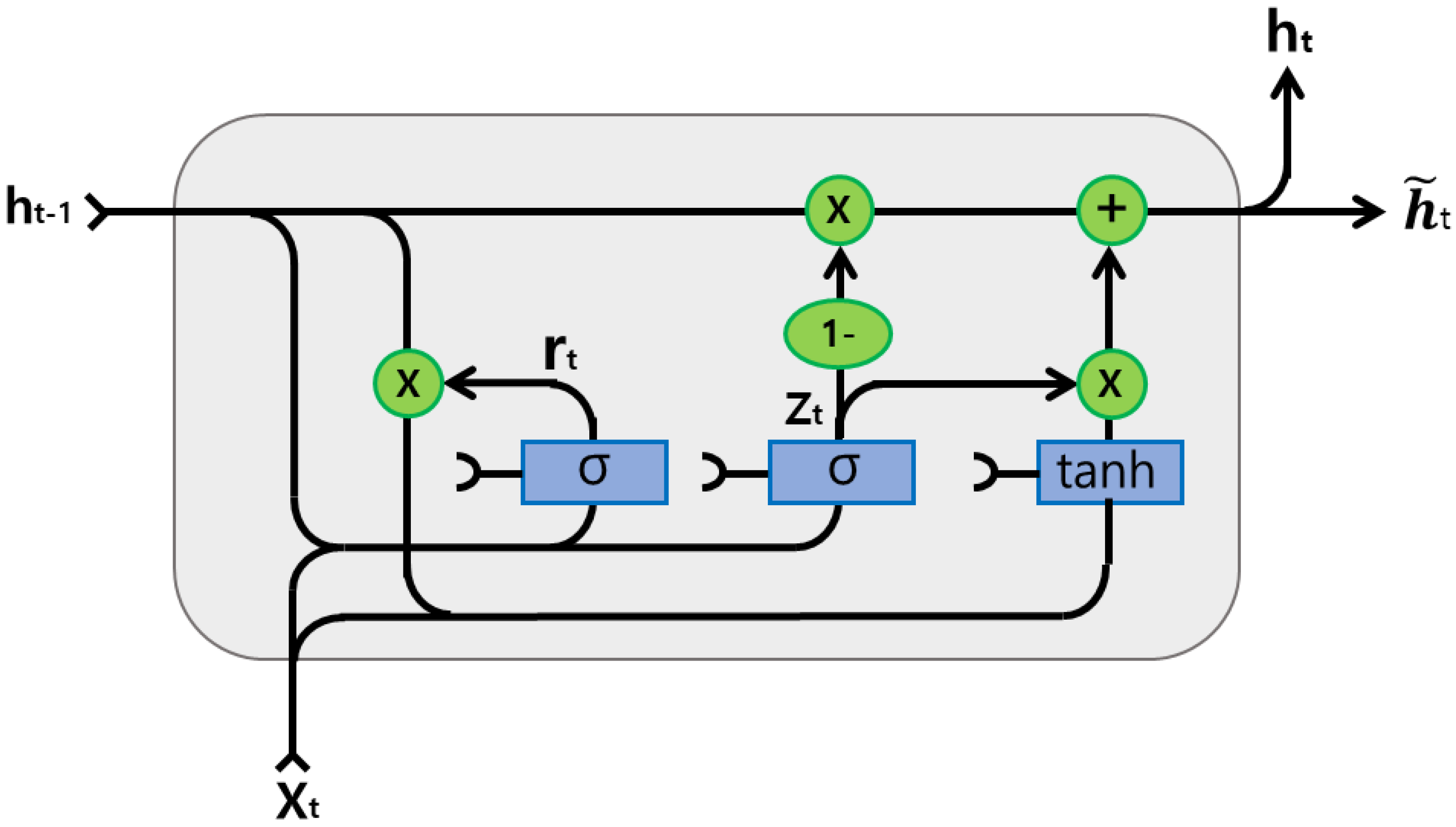
GRU developed to solve the long short dependency problem regarding vanishing and exploding gradients, which is another well-known version of LSTM [10]. GRU is concretely designed to handle sequential data that shows patterns over time steps, such as time-series data. The structure of GRU, which consists of an update gate and a reset gate, is simpler than LSTM which has three gates, an input gate, a forget gate, and an output gate. Thus, the train speed of GRU is a little bit faster than LSTM.
The update gate controls how much information should be added at the next state cell. More information moves into the next state cell when the value of the update gate is higher. The reset gate controls how much of the previous information should be forgotten. In this case, more information from the previous cell might be forgotten when the value of the reset gate is higher [27]. The equations for update gate and reset gate are explained below:
The hidden state related to current time step takes a linear interpolation between the previous activation function at previous time step and the candidate hidden state . Both the hidden state and the candidate hidden state are formulated as:
In Equations (1)–(4), the matrices , , and are the input weighted matrices, and , , and are the recurrent weight matrices. The vectors and are the bias vectors. The function is the activation function. Figure 1 shows the structure of GRU.
3.2. Genetic Algorithm
GA is one of the famous meta heuristic algorithms based on a stochastic optimization method. The major benefit of GA is to obtain an optimal or a near optimal solution of a large scale problem under reasonable computing time [28]. Holland [29] developed GA based on Darwin’s The Origin of Species, so it utilizes natural evolution. GA begins with a set population, which is the initial set of random solutions. And then, GA selects chromosomes to obtain a good fitness value. For this process, GA consists of three operators: selection, crossover, and mutation. Thus, the efficiency of GA depends on the initial population and those operators. The three operators and fitness functions of GA are described as follows.
3.2.1. Selection
Using the selection operator, GA picks good chromosomes for the next generation. Tournament selection is used in this paper. This selection is done by running several tournaments among certain chromosomes which are randomly picked from the population. The winning chromosome of each tournament with the best fitness value is selected, and those chromosomes move into the next generation.
3.2.2. Crossover
For producing offspring chromosomes, the crossover operator is performed between parent chromosomes. The two points crossover is applied in this paper. This crossover randomly picks two crossover points from parent chromosomes and swaps them [30].
3.2.3. Mutation
The mutation operator randomly changes one or more genes in a chromosome. Due to this operator, GA can escape the local optimum. We use the uniform mutation operator which changes the value of chosen genes to a random uniform value [31].
3.2.4. Fitness Function
Evaluating the performance of GA, we calculate a fitness value using a fitness function. We apply two kinds of evaluation functions; root mean square error (RMSE) and mean absolute error (MAE). Those equations are presented as follows:
In Equations (5) and (6), is the number of data values in the time-series. and denote the real value and predicted value, respectively. Finally, the process of GA is presented as follows:
- Step 1.
- (Initialization)
- Step 1.1
- Set = 1.
- Step 1.2
- Set length of chromosome , range of gene value , population size , probability of crossover , mutation factor , maximum iteration number .
- Step 1.3
- Search the initial population randomly.
where - Step 2.
- Calculate the fitness function an Equation (5) or (6) for each chromosome .
- Step 3.
- (Apply the tournament selection operator)
- Select two chromosomes and which have good fitness values.
- Step 4.
- (Apply the crossover operator with )
- Select two-points randomly and swap chromosomes, and .
- Step 5.
- (Apply the mutation operator)
- Step 5.1
- Set the definition domain of each gene, , as rand .
- Step 5.2
- For = 1 to , if the definition domain of < ,
- Step 6.
- If , and go to Step 2. Otherwise, stop GA.
3.3. Hyperparameter Optimization Using Genetic Algorithm
In this section, we develop a hybrid model GA-GRU to obtain the hyperparameters of GRU using GA. The NN based models, such as ANN, RNN, LSTM, GRU, etc., have a lot of hyperparameters which affect their performance. A decision maker sets hyperparameters using the rule of thumb method before the machine learning process is started. Regarding this, a decision maker who has less experience would be likely to obtain bad results. Finding optimal hyperparameters is one of the major issues in machine learning. However, finding optimal hyperparameters is a non-deterministic polynomial (NP) hard problem, which is difficult to solve. GA is a well-known powerful meta-heuristic algorithm used to solve NP problems in a variety of fields [32]. Therefore, we apply GA when searching for optimal hyperparameters for GRU.
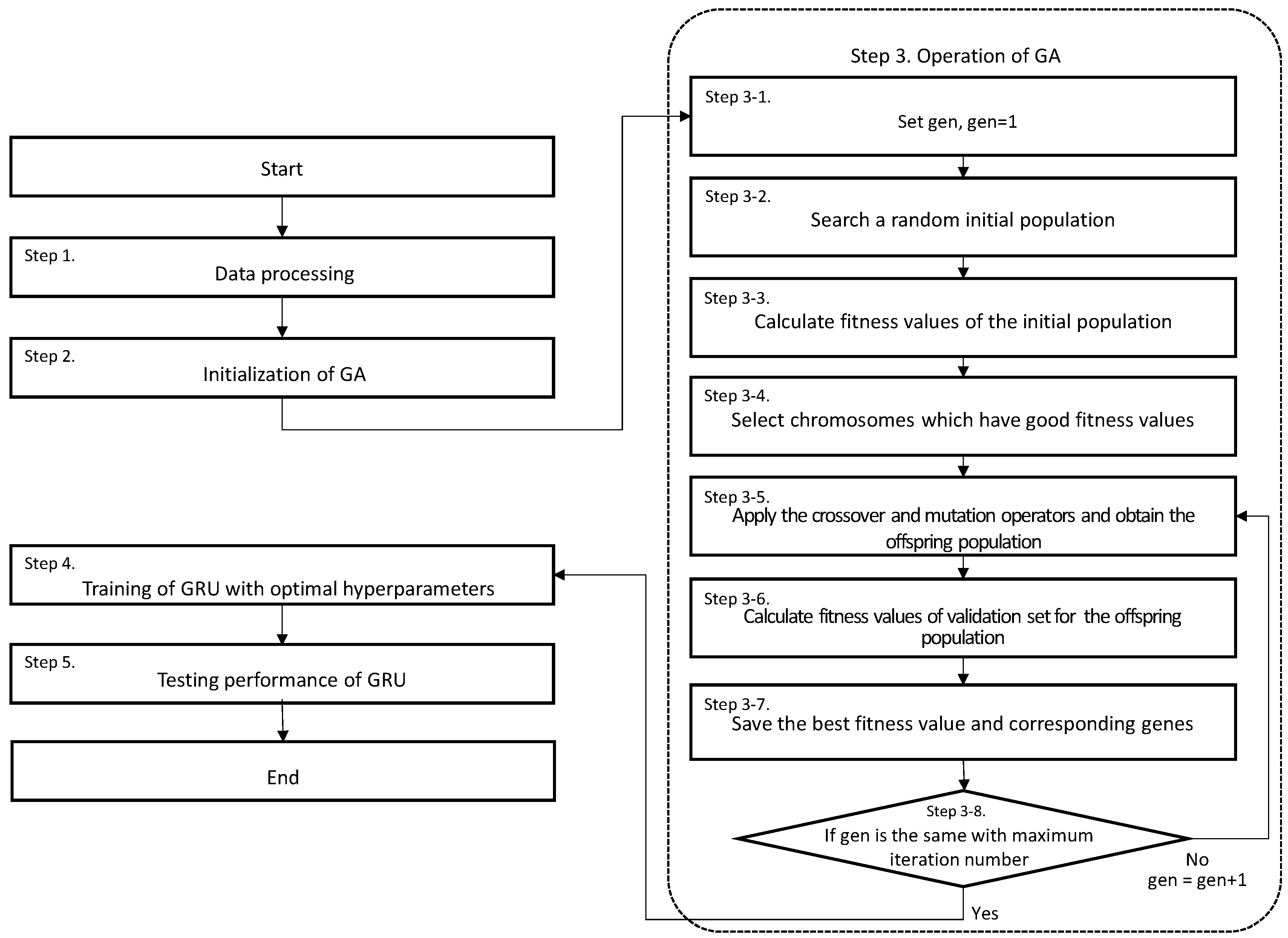
In this paper, we focus on five hyperparameters: window size, number of neurons in the hidden state, batch size, epoch size, and initial learning rate. First is the window size, which is normally called the length of the input. A suitable length of the input can keep necessary input data which reduces forecasting errors. Second is the number of neurons in the hidden state. Using few neurons in the hidden state causes underfitting, and vice versa. Third is the batch size. If the batch size is small, the training might be underfitted. If the batch size is large, we need a lot of required memory. Fourth is the epoch size. If the epoch size is small, the learning has difficulty converging. If the epoch size is large, the training might be overfitted. Fifth is the initial learning rate. An over or under sized learning rate can cause undesirable divergence in the short time and tapping in local minima with long time. Even though some methods, which change the learning rate during the learning process, are developed, setting the initial learning rate is still important. As we mentioned above, the performance of GRU can be affected by the five hyperparameters. Thus, the purpose of GA-GRU is to optimize those hyperparameters using GA. Figure 2 shows the flowchart of GA-GRU. The main procedure of GA-GRU is proposed as follows:
- Step 1.
- (Data processing)
- The dataset is normalized and then divided into training, validation, and test sets.
- Step 2.
- (Initialization of GA)
- Set
- Set length of chromosome , range of gene value , population size , probability of crossover, mutation factor, maximum iteration number .
- Step 3.
- (Operation of GA)
- Step 3.1 Set gen = 1
- Step 3.2 Search a random initial population.
- where
- Step 3.3 Calculate fitness values for the initial population using Equation (5) or (6).
- Step 3.4 Select chromosomes which have good fitness values.
- Step 3.5 (Apply the crossover and mutation operators and obtain the offspring population)
- Step 3.5.1 Select two-points randomly and swap chromosomes.
- Step 3.5.2 Set the definition domain of each gene, , as rand .
- Step 3.5.3 For = 1 to , if the definition domain of < ,
- Step 3.5.4 Generate new offspring population.
- Step 3.6 Using Equation (5) or (6), calculate the fitness values of the validation set for the offspring population.
- Step 3.7 Set
- Step 3.8 If gen = , GA is terminated. Otherwise, gen = gen + 1, and go to Step 3–5.
- Step 4.
- (Training of GRU with optimal hyperparameters)
- GRU with optimal hyperparameters is trained using the training and validation sets.
- Step 5.
- (Testing performance of GRU)
- Compare the test set with the forecasting outputs of GRU.
In Step 1, the dataset is normalized and then divided into three main datasets, training (70% of the dataset), validation (10% of the dataset), and test (20% of the dataset). In Step 2, the parameters of GA are initialized. In Step 3, GA searches hyperparameters and applies them to train a GRU model with the training set. While training a GRU model, we use mean squared error (MSE) as a loss function. Then, using the validation set, GA calculates a fitness function with the current hyperparameters. Equation (7) denotes the function of MSE.
GA ends when the current generation hits the maximum generation, otherwise GA moves to the next generation in order to find a better solution. Step 4 is to train a GRU model with optimal hyperparameters using the training and validation sets. In Step 5, GRU obtains the predicted vales and compares them with the test set.
4. Experiments
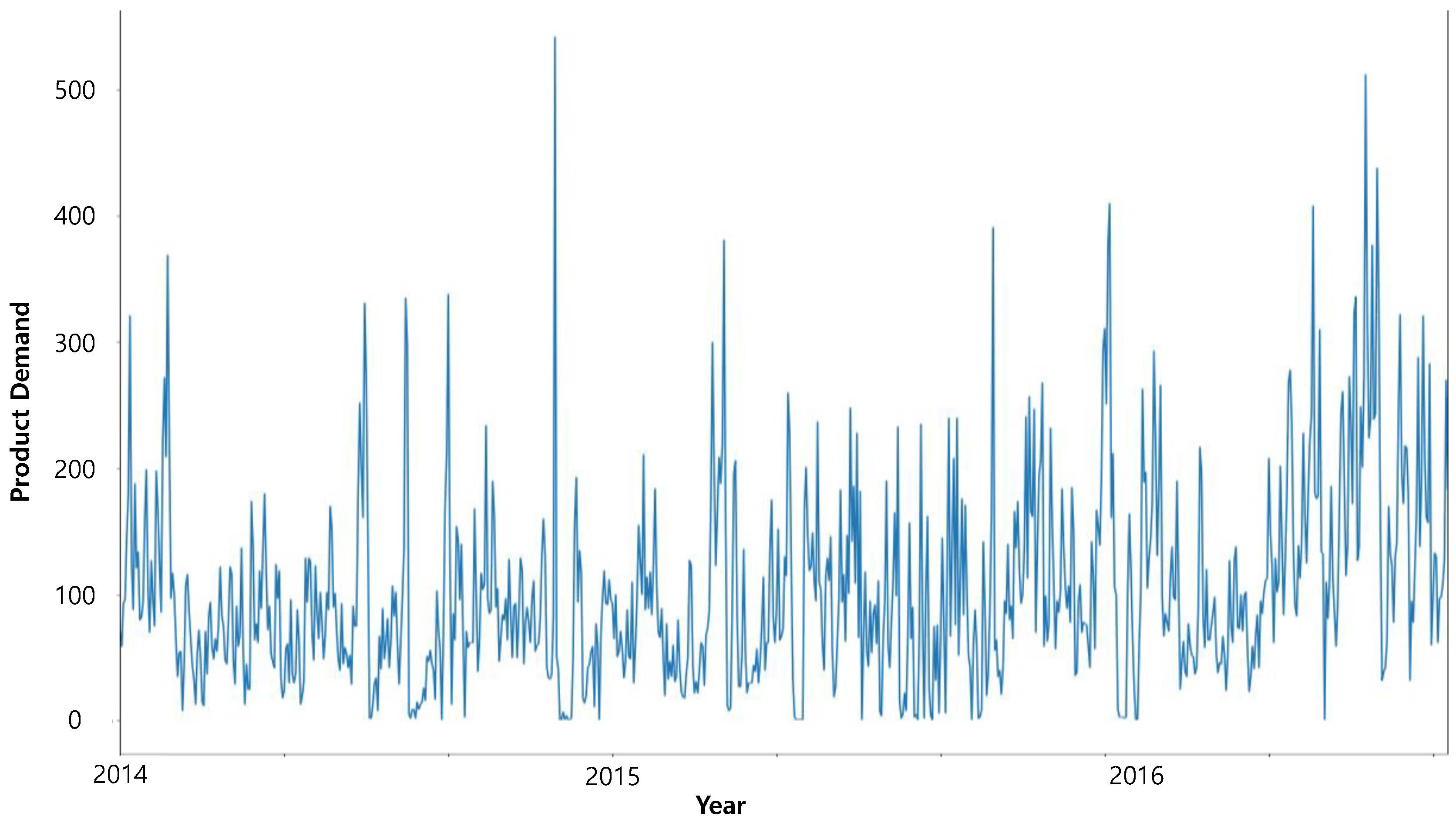
To check the performance of GA-GRU, we performed three experiments. The first experiment was to compare GA-GRU with other models, such as ARIMA, ANN, RNN, and GA-LSTM. The second experiment was to test k-fold cross validation. The third experiment was the sensitive analysis of the GA parameters. We took a Brazilian top retailer’s sales dataset, which included the customers’ daily product demand, from January 2014 to July 2016 (Retail Sales Forecasting, https://www.kaggle.com/tevecsystems/retail-sales-forecasting) as an example. The dataset was divided into three subsets: training set (70%, 564 observations), validation set (10%, 81 observations), and test set (20%, 162 observations). Because the dataset was daily demand data, 1-day-ahead (one-step-ahead) forecasting was performed. Figure 3 shows the time-series graph of daily product demand.
Before we performed the three experiments using the dataset, data preprocessing had to be applied. This work is one of the important steps for obtaining better performance and accuracy, because the data has some missing fields and noise. The data has different scales, so the features with a large scale might dominate other features. This situation weakens learning performance. Thus, using the normalization method, we made the data the same scale, which means each sample is equally important. In this paper, the raw dataset was preprocessed through the min-max normalization method. The equation of the min-max normalization method is presented as follows [24]:
In Equation (8), is the original data of the raw dataset. and are the maximum value of the features and the minimum value of the features, respectively. is the normalized value, scaled to be . The optimizer is an adaptive moment estimation (ADAM) optimizer. We used a computer with an Intel i7 3770 3.9GHZ, 16GB RAM, and a NVIDIA Geforce GTX 1060 graphics card. The development environment is Python 3.6 where GRU is implemented with Tensorflow 2.0. For GA, we utilized Distributed Evolutionary Algorithms in Python (DEAP). To obtain optimal hyperparameters, it is necessary to set the range for each hyperparameter on the search space of GA. It is recommended that the ranges of hyperparameters, such as window size, number of neurons in the hidden state, batch size, and epoch size, are set as less than the range of the training set (observation). The initial learning rate should be less than 1. It is better to decide those ranges based on personal computer performance, because large ranges require more memory and computational time. Table 1 shows the range of each hyperparameter of GRU used in this paper.
4.1. Comparison of the Performance of GA-GRU with other Forecasting Models
This test compared GA-GRU with five forecasting models including ARIMA, RNN, LSTM, GRU, and GA-LSTM. GA-LSTM is a hybrid model operated as the same manner as GA-GRU. We applied GA to LSTM to find five hyperparameters of LSTM. To evaluate the performance of those models, we used two measures, RMSE and MAE. Table 2 presents the parameters of GA used in this experiment.
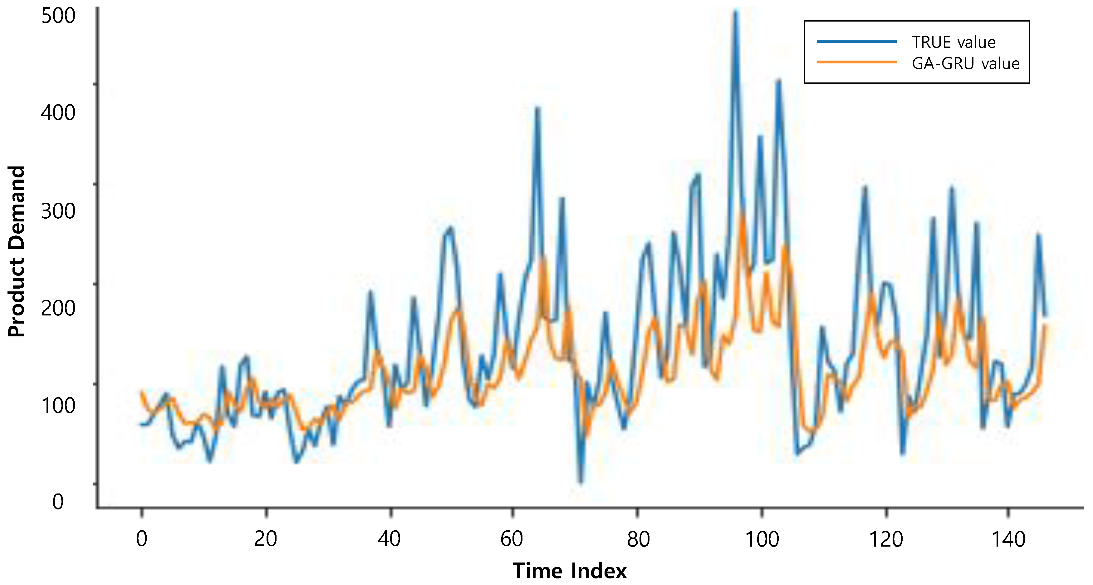
The parameters of GA were set based one previous research. GA obtains poor results with a very small population and small generation number. According to Kalyanmoy and Samir (1999), the population size and generations should be set to 5 or more and larger than the population size, respectively. Based on this, we set population size at 10 and number of generations at 15. In addition, the crossover probabilities and mutation factors in the literature are generally set as 0.5–1.0 and 0.005–0.05, respectively [33]. On the basis of similar work [24], crossover probability and mutation factor were set at 0.7 and 0.015, respectively. Table 3 reports the performance of the six forecasting models. Compared with different forecasting models, GA-GRU achieves higher accuracy in the cases of RMSE and MAE. The measure is defined as a percent deviation, where is the result of GA-GRU, and is the result of other forecasting models. This measure proves that GA can obtain optimal hyperparameters of GRU. In addition, the interesting point is that GA-GRU obtains better results than GA-LSTM although the hyperparameters of both models are optimized using GA. This result shows that GRU is more powerful than LSTM in our problem. In short, GA-GRU dominated other forecasting models. Figure 4 illustrates the comparison graph of actual demand and forecasted demand generated by GA-GRU.
4.2. Test the k-Fold Cross-Validation of GA-GRU
We checked the k-fold cross-validation which splits the time-series dataset into k-fold subsets. This method repeats the process of splitting the dataset into training and test sets k-times. The size of the test set is fixed while the size of the training set increases for every fold. Testing the cross-validation offers a robust performance estimation of demand forecasting when each data is used for training and testing at each k-fold [24]. We utilized 10-fold cross-validation using the best hyperparameters of GA-GRU obtained in Section 4.1.
Table 4 shows the result of the 10-fold cross-validation. The results of RMSE and MAE in each fold are different because both train and test sets are shuffled during the test of k-fold cross-validation. This test improved the confidence of forecasting efficiency even though the dataset is small. When the dataset is small, the overfitting will result. The k-fold cross-validation can check the overfitting of current GA-GRU model which obtains optimal hyperparameters. The mean of RMSE and MAE in the 10-fold cross-validation is less than the results of GA-GRU in Section 4.1. Thus, the GA-GRU with optimal hyperparameters is not overfitted even though we trained GA-GRU with small datasets.
4.3. Sensitivity Analysis of the Genetic Algorithm Parameters
The results of GA-GRU are affected by the GA parameters such as probability of crossover and mutation factor. In this experiment, we tested the forecasting accuracy between the performance of GA-GRU and the GA parameters. The results of the sensitivity analysis are presented in Table 5 and Table 6.
Table 5 shows the forecasting results at different mutation factors. When the mutation factor is 0.015, both RMSE and MAE are minimized. Table 6 shows the forecasting results of different crossover probabilities. When the probability of crossover is 0.70, both RMSE and MAE are minimized. It is important to calculate the proper crossover probability and mutation factor, because those parameters affect the performance of GA. According to the literature [33], large crossover probability can converge a population quickly but might miss the optimal solution. A large mutation factor changes GA to a purely random search algorithm. In this sensitivity analysis, the result suggests setting the mutation factor to 0.015 and the probability of crossover to 0.70. Even though the optimal values of those parameters might change depending on the dataset, this result will help a decision maker who sets GA parameters when he/she faces this kind of problem.
5. Implications
5.1. Academic Implications
This paper suggested a hybrid model that combined GRU and GA for product demand forecasting in SCM. Even though GRU has been a well-known NN model in the time-series forecasting area, it is quite difficult to set the initial hyperparameters for improved performance. Accordingly, we suggested that GA obtain the optimal hyperparameters of GRU. This is the first attempt to consider five hyperparameters including window size, number of neurons in the hidden state, batch size, epoch size, and initial learning rate. We believe that this research is an initiating academic research in the area of product demand forecasting and hyperparameter selection. Thus, this research will help other researchers who want to study related follow-up problems.
5.2. Managerial Implications
The proposed GA-GRU provides valuable implications for a company by predicting future product demand. Based on product demand forecasting, the company can do inventory control and make a cost-minimizing business plan. Because GA-GRU finds the optimal hyperparameters of GRU, GA-GRU has the advantages of flexibility and customization. As an example, a company can combine GA-GRU with a parallel computing technique and frameworks, such as MapReduce, Hadoop, and Spark. Applying a parallel computing technique to GA-GRU can handle time series data sets in real time. In addition, GA-GRU could be applied for forecasting any industry area such as inventory, demand, sales, and pricing. Accordingly, the company can apply GA-GRU to various complex business situations. Thus, the company could obtain the basis of decision making and respond to future uncertainty.
6. Conclusions and Future Researches
This paper presents a hybrid model called GA-GRU, which predicts future product demand in SCM. Due to false demand forecasting driving up a lot of supply chain costs, many companies and researchers have focused on methods of demand forecasting. In order to improve the performance of demand forecasting, we developed GA-GRU based on two research ideas. First is to utilize GRU. GRU is an upgraded version of LSTM and has an advantage in handling time-series data. Second is to apply GA to GRU. GA is a well-known meta-heuristic algorithm in various research areas. The performance of GRU is dependent on the initial hyperparameter values. If the hyperparameters of GRU are set incorrectly, the demand forecasting performance might be bad. We considered five hyperparameters of GRU, window size, number of neurons in the hidden state, batch size, epoch size, and initial learning rate. Thus, GA-GRU firstly obtains optimal hyperparameter values, then operates the process of demand forecasting.
To test the performance and accuracy of GA-GRU, we conducted three experiments. First, we compared GA-GRU with five forecasting models including ARIMA, RNN, LSTM, GRU, and GA-LSTM. Although GA-LSTM followed the same process as GA-GRU, GA-GRU gets better results. It suggests that GRU is more powerful than LSTM in our problem. Also, the result shows that GA-GRU dominates the other five forecasting models. Second, we performed 10-fold cross-validation testing. Based on this test, we showed the robust performance of GA-GRU. Third, we performed a sensitivity analysis of the GA parameters. GA-GRU is functionally an optimization-based model for product demand forecasting using GA and GRU. The performance of GA-GRU is dependent on the GA parameters. The result shows that setting the mutation factor of 0.015 and the crossover probability of 0.70 is the best option. This experiment might be useful for a decision maker who is a beginner in GA.
There are some limitations of our research and related future research topics. First, this paper only considers univariate time-series data. For handling more complex supply chain problems, we could consider multivariate time-series data. Second, we only focused on a single GRU model. In order to improve the performance of forecasting, GRU can be combined with other models such as ARIMA and convolutional NN, etc. Finally, other meta-heuristic algorithms can be applied in order to obtain optimal hyperparameter values.
Author Contributions
Conceptualization, J.N. and J.S.K.; Funding acquisition, S.-J.H.; Methodology, J.N. and S.-J.H.; Software, J.N.; Validation, H.-J.P.; Visualization, H.-J.P.; Writing—original draft, J.N.; Writing—review & editing, H.-J.P.. All authors have read and agreed to the published version of the manuscript.
Funding
This work was supported by the Ministry of Education of the Republic of Korea and the National Research Foundation of Korea (NRF-2019S1A5C2A04083153).
Conflicts of Interest
The author declares no conflict of interest.
References
- Chawla, A.; Singh, A.; Lamba, A.; Gangwani, N.; Soni, U. Demand forecasting using artificial neural networks—A case study of american retail corporation. In Applications of Artificial Intelligence Techniques in Engineering; Springer: Singapore, 2019; pp. 79–89. [Google Scholar]
- Kilimci, Z.H.; Akyuz, A.O.; Uysal, M.; Akyokus, S.; Uysal, M.O.; Atak Bulbul, B.; Ekmis, M.A. An improved demand forecasting model using deep learning approach and proposed decision integration strategy for supply chain. Complexity 2019, 2019, 9067367. [Google Scholar] [CrossRef] [Green Version]
- Weng, T.; Liu, W.; Xiao, J. Supply chain sales forecasting based on lightgbm and LSTM combination model. Ind. Manag. Data Syst. 2019, 120, 265–279. [Google Scholar] [CrossRef]
- Kim, M.; Jeong, J.; Bae, S. Demand Forecasting Based on Machine Learning for Mass Customization in Smart Manufacturing. In Proceedings of the 2019 International Conference on Data Mining and Machine Learning, Hong Kong, China, 28–30 April 2019; pp. 6–11. [Google Scholar]
- Chen, T.; Yin, H.; Chen, H.; Wang, H.; Zhou, X.; Li, X. Online sales prediction via trend alignment-based multitask recurrent neural networks. Knowl. Inf. Syst. 2019, 1–29. [Google Scholar] [CrossRef]
- Hochreiter, S.; Schmidhuber, J. Long short-term memory. Neural Comput. 1997, 9, 1735–1780. [Google Scholar] [CrossRef] [PubMed]
- Yousfi, S.; Berrani, S.-A.; Garcia, C. Contribution of recurrent connectionist language models in improving LSTM-based arabic text recognition in videos. Pattern Recognit. 2017, 64, 245–254. [Google Scholar] [CrossRef]
- Pham, T.; Tran, T.; Phung, D.; Venkatesh, S. Predicting healthcare trajectories from medical records: A deep learning approach. J. Biomed. Inform. 2017, 69, 218–229. [Google Scholar] [CrossRef]
- Evermann, J.; Rehse, J.-R.; Fettke, P. Predicting process behaviour using deep learning. Decis. Support Syst. 2017, 100, 129–140. [Google Scholar] [CrossRef] [Green Version]
- Cho, K.; Van Merriënboer, B.; Gulcehre, C.; Bahdanau, D.; Bougares, F.; Schwenk, H.; Bengio, Y. Learning phrase representations using rnn encoder-decoder for statistical machine translation. arXiv 2014, arXiv:1406.1078. [Google Scholar]
- Bandara, K.; Shi, P.; Bergmeir, C.; Hewamalage, H.; Tran, Q.; Seaman, B. International Conference on Neural Information Processing. In Sales Demand Forecast in E-Commerce Using a Long Short-Term Memory Neural Network Methodology; Springer: Cham, Switzerland, 2019; pp. 462–474. [Google Scholar]
- Peng, L.; Liu, S.; Liu, R.; Wang, L. Effective long short-term memory with differential evolution algorithm for electricity price prediction. Energy 2018, 162, 1301–1314. [Google Scholar] [CrossRef]
- Sagheer, A.; Kotb, M. Time series forecasting of petroleum production using deep LSTM recurrent networks. Neurocomputing 2019, 323, 203–213. [Google Scholar] [CrossRef]
- Bouktif, S.; Fiaz, A.; Ouni, A.; Serhani, M.A. Optimal deep learning LSTM model for electric load forecasting using feature selection and genetic algorithm: Comparison with machine learning approaches. Energies 2018, 11, 1636. [Google Scholar] [CrossRef] [Green Version]
- Kim, J.S.; Shin, K.Y.; Ahn, S.-E. A multiple replenishment contract with ARIMA demand processes. J. Oper. Res. Soc. 2003, 54, 1189–1197. [Google Scholar] [CrossRef]
- Shukla, M.; Jharkharia, S. ARIMA models to forecast demand in fresh supply chains. Int. J. Oper. Res. 2011, 11, 1–18. [Google Scholar] [CrossRef]
- Babai, M.Z.; Ali, M.M.; Boylan, J.E.; Syntetos, A.A. Forecasting and inventory performance in a two-stage supply chain with ARIMA (0, 1, 1) demand: Theory and empirical analysis. Int. J. Prod. Econ. 2013, 143, 463–471. [Google Scholar] [CrossRef]
- Ramos, P.; Santos, N.; Rebelo, R. Performance of state space and ARIMA models for consumer retail sales forecasting. Robot. Comput. Integr. Manuf. 2015, 34, 151–163. [Google Scholar] [CrossRef] [Green Version]
- Van Calster, T.; Baesens, B.; Lemahieu, W. ProfARIMA: A profit-driven order identification algorithm for ARIMA models in sales forecasting. Appl. Soft Comput. 2017, 60, 775–785. [Google Scholar] [CrossRef] [Green Version]
- Panapakidis, I.P.; Dagoumas, A.S. Day-ahead electricity price forecasting via the application of artificial neural network based models. Appl. Energy 2016, 172, 132–151. [Google Scholar] [CrossRef]
- Keles, D.; Scelle, J.; Paraschiv, F.; Fichtner, W. Extended forecast methods for day-ahead electricity spot prices applying artificial neural networks. Appl. Energy 2016, 162, 218–230. [Google Scholar] [CrossRef]
- Gensler, A.; Henze, J.; Sick, B.; Raabe, N. Deep learning for solar power forecasting—An approach using autoencoder and LSTM neural networks. In Proceedings of the 2016 IEEE international Conference on Systems, Man, and Cybernetics (SMC), Budapest, Hungary, 9–12 October 2016; pp. 2858–2865. [Google Scholar]
- Choi, J.Y.; Lee, B. Combining LSTM network ensemble via adaptive weighting for improved time series forecasting. Math. Probl. Eng. 2018, 2018, 2470171. [Google Scholar] [CrossRef] [Green Version]
- Almalaq, A.; Zhang, J.J. Evolutionary deep learning-based energy consumption prediction for buildings. IEEE Access 2018, 7, 1520–1531. [Google Scholar] [CrossRef]
- Su, H.; Zio, E.; Zhang, J.; Xu, M.; Li, X.; Zhang, Z. A hybrid hourly natural gas demand forecasting method based on the integration of wavelet transform and enhanced deep-rnn model. Energy 2019, 178, 585–597. [Google Scholar] [CrossRef] [Green Version]
- Kochak, A.; Sharma, S. Demand forecasting using neural network for supply chain management. Int. J. Mech. Eng. Obotics Res. 2015, 4, 96–104. [Google Scholar]
- Tang, Y.; Huang, Y.; Wu, Z.; Meng, H.; Xu, M.; Cai, L. Question detection from acoustic features using recurrent neural network with gated recurrent unit. In Proceedings of the 2016 IEEE International Conference on Acoustics, Speech and Signal Processing (ICASSP), Shanghai, China, 20–25 March 2016; pp. 6125–6129. [Google Scholar]
- Noh, J.; Kim, J.S. Cooperative green supply chain management with greenhouse gas emissions and fuzzy demand. J. Clean. Prod. 2019, 208, 1421–1435. [Google Scholar] [CrossRef]
- Holland, J.H. Adaptation in Natural and Artificial Systems: An Introductory Analysis with Applications to Biology, Control, and Artificial Intelligence; MIT Press: Cambridge, MA, USA, 1992. [Google Scholar]
- Kaya, M. The effects of two new crossover operators on genetic algorithm performance. Appl. Soft Comput. 2011, 11, 881–890. [Google Scholar] [CrossRef]
- Eiben, A.E.; Smith, J.E. Introduction to Evolutionary Computing; Springer: Berlin, Germany, 2003; Volume 53. [Google Scholar]
- Gen, M.; Lin, L. Genetic algorithms. In Wiley Encyclopedia of Computer Science and Engineering; Wiley-Interscience: Hoboken, NJ, USA, 2007; pp. 1–15. [Google Scholar]
- Kalyanmoy, D.; Samir, A. Understanding interactions among genetic algorithm parameters. In Foundations of Genetic Algorithms V; Morgan Kauffman: San Mateo, CA, USA, 1999; pp. 265–286. [Google Scholar]
Figure 1.
The structure of Gated Recurrent Unit.

Figure 2.
The flowchart of GA-GRU.

Figure 3.
Time-series graph of daily product demand.

Figure 4.
The graph of the forecasted demand generated by GA-GRU and real demand.


Table 1.
The range of hyperparameters of Gated Recurrent Unit.
| Hyperparameter | Range |
|---|---|
| Window size | |
| Number of neurons in the hidden state | |
| Batch size | |
| Epoch size | |
| Initial learning rate | |
| Loss function | MSE |
Table 2.
The parameters of Genetic Algorithm.
| Parameter | Value |
|---|---|
| Number of population size | 10 |
| Number of generations | 15 |
| Crossover probability | 0.70 |
| Mutation factor | 0.015 |
Table 3.
The performance of different forecasting models.
| Forecasting Model | RMSE | Percent Deviation | MAE | Percent Deviation |
|---|---|---|---|---|
| ARIMA | 96.494 | −24.312 | 69.723 | −27.013 |
| RNN | 84.900 | −13.985 | 61.380 | −17.092 |
| LSTM | 83.315 | −12.348 | 58.045 | −12.328 |
| GRU | 81.341 | −10.221 | 56.423 | −9.808 |
| GA-LSTM | 80.729 | −9.541 | 51.996 | −2.129 |
| GA-GRU | 73.027 | . | 50.889 | . |
Table 4.
The results of the 10-fold cross-validation.
| Number of Folds | RMSE | MAE |
|---|---|---|
| 1 | 53.214 | 39.660 |
| 2 | 47.354 | 37.817 |
| 3 | 60.134 | 43.875 |
| 4 | 71.770 | 42.149 |
| 5 | 53.064 | 40.836 |
| 6 | 64.976 | 52.274 |
| 7 | 75.330 | 60.632 |
| 8 | 63.977 | 48.907 |
| 9 | 50.466 | 37.180 |
| 10 | 96.630 | 63.324 |
| Mean | 63.692 | 46.665 |
| Standard deviation | 14.016 | 8.880 |
Table 5.
The forecasting results with different mutation factors.
| Probability of Crossover | Mutation Factor | RMSE | MAE |
|---|---|---|---|
| 0.70 | 0.005 | 74.315 | 51.957 |
| 0.010 | 73.673 | 51.086 | |
| 0.015 | 73.027 | 50.889 | |
| 0.020 | 74.272 | 51.391 | |
| 0.025 | 74.507 | 51.045 |
Table 6.
The forecasting results with different probabilities of crossover.
| Mutation Factor | Probability of Crossover | RMSE | MAE |
|---|---|---|---|
| 0.015 | 0.60 | 74.681 | 52.321 |
| 0.65 | 74.220 | 51.040 | |
| 0.70 | 73.027 | 50.889 | |
| 0.75 | 73.926 | 51.061 | |
| 0.80 | 74.261 | 51.582 |
© 2020 by the authors. Licensee MDPI, Basel, Switzerland. This article is an open access article distributed under the terms and conditions of the Creative Commons Attribution (CC BY) license (http://creativecommons.org/licenses/by/4.0/).
Share and Cite
MDPI and ACS Style
Noh, J.; Park, H.-J.; Kim, J.S.; Hwang, S.-J. Gated Recurrent Unit with Genetic Algorithm for Product Demand Forecasting in Supply Chain Management. Mathematics 2020, 8, 565. https://0-doi-org.brum.beds.ac.uk/10.3390/math8040565
AMA Style
Noh J, Park H-J, Kim JS, Hwang S-J. Gated Recurrent Unit with Genetic Algorithm for Product Demand Forecasting in Supply Chain Management. Mathematics. 2020; 8(4):565. https://0-doi-org.brum.beds.ac.uk/10.3390/math8040565
Chicago/Turabian StyleNoh, Jiseong, Hyun-Ji Park, Jong Soo Kim, and Seung-June Hwang. 2020. "Gated Recurrent Unit with Genetic Algorithm for Product Demand Forecasting in Supply Chain Management" Mathematics 8, no. 4: 565. https://0-doi-org.brum.beds.ac.uk/10.3390/math8040565
Note that from the first issue of 2016, this journal uses article numbers instead of page numbers. See further details here.