A Decentralized Framework for Parameter and State Estimation of Infiltration Processes

Abstract

The Richards’ equation is widely used in the modeling soil water dynamics driven by the capillary and gravitational forces in the vadose zone. Its state and parameter estimation based on field soil moisture measurements is important and challenging for field applications of the Richards’ equation. In this work, we consider simultaneous state and parameter estimation of systems described by the three dimensional Richards’ equation with multiple types of soil. Based on a study on the interaction between subsystems, we propose to use decentralized estimation schemes to reduce the complexity of the estimation problem. Guidelines for subsystem decomposition are discussed and a decentralized estimation scheme developed in the framework of moving horizon state estimation is proposed. Extensive simulation results are presented to show the performance of the proposed decentralized approach.

1. Introduction

Agriculture accounts for about 70% consumed fresh water according to the United Nations statistics [1]. However, the average water-use efficiency in agriculture irrigation is about 50% globally [2]. In order to achieve water sustainability, it is important to significantly improve the water-use efficiency in agriculture irrigation. If we examine the current irrigation practice from a systems engineering perspective, majority of irrigation currently is done in an open-loop manner, in which no real-time field measurement (e.g., soil moisture) is used in irrigation decision making. The current open-loop irrigation leads to excessive consumption of water resources. Closed-loop irrigation, in which real-time field measurements are used to determine the time and the amount of water to be applied, is a promising alternative to significantly reduce water consumption. In the implementation of a closed-loop irrigation system, the soil moisture information of the entire field is important. It is, however, very expensive to install sufficient number of sensors to cover one agriculture field. One approach to conquer this challenge is to use a model of the field and state estimate to reconstruct the soil moisture of the entire field based on the measurements of a small number of sensors. In this work, we focus on infiltration processes that can be described by the Richards’ equation and consider simultanesouly online estimation of soil moisture and soil parameters online.

For online soil state and parameter estimation, sequential data assimilation is one commonly used type of approaches. Generally, in this type of approaches, the first step is to use a dynamical model of the infiltration process to predict the current soil state; and then, in the second step, the prediction is corrected based on process measurements. Kalman filter and its variants are the most widely adopted algorithms in implementing the prediction-update approach (e.g., [3,4,5,6,7,8]). When estimating soil parameters using sequential data assimilation, parameters are typically augmented as extra states of the dynamical model. For example, Li and Ren [9] studied parameter estimation by augmenting parameters as states and used ensemble Kalman filter (EnKF) as the estimation algorithm. In [5], dual Kalman filter was used to first estimate the states using a standard Kalman filter and then to estimate the parameters using an unscented Kalman filter. In [7], three ensemble-based simultaneous state and parameter estimation methods, augmented ensemble Kalman filter, dual EnKF and simultaneous optimization and data assimilation were compared. The augmented EnKF was found to be the most robust method for general conditions. However, the above discussed methods do not handle constraints on the states or parameters in a systematical way. Constraints on the states and parameters may contain important information and may be used to significantly improve estimation performance. In our previous work [10], we compared the estimation performance of the moving horizon estimation (MHE), extended Kalman filter (EKF) and ensemble Kalman filter (EnKF) on a one-dimensional (1D) infiltration process. It showed that MHE outperforms the other two on parameter and state estimation due to the consideration of constraints on state and parameters.

Moving horizon estimation is an online optimization-based estimation method, which is widely used in state estimation of nonlinear systems [11,12]. Since MHE casts an estimation problem into an optimization-based problem, the computational complexity is typically much higher than that of other common estimation algorithms. Therefore, when dealing with systems/processes of medium to large scales, centralized MHE may fail to provide online estimates due to increasingly high computational load; this issue is especially significant for systems with complex nonlinearity like the infiltration processes considered in this work. In addition to concerns about the computational load, the centralized structure that exploits one single agent to handle plant-wide tasks is not favorable from the perspectives of fault tolerance, organizational and maintenance flexibility [13,14,15,16,17]. The above considerations have motivated the use of decentralized and distributed frameworks in advanced control [18,19,20,21] as well as state estimation [22,23,24,25]. In a decentralized/distributed context, the overall system/process is typically divided into smaller units (subsystems), and the original estimation problem which could be large and complex is typically decomposed into smaller sub-problems, which are handled by a number of local agents instead of using a single central agent. In this way, the computational burden for each agent is eased, and the fault tolerance and maintenance flexibility can be much enhanced at the same time. While the decentralized and the distributed frameworks are inherently similar, one primary difference between them is that the local agents of a decentralized scheme typically do not communicate with each other while the local agents of a distributed scheme coordinate with each other via communication. As a result, a distributed architecture can be advantageous when the sub-problems have significant interaction; that is, when the subsystems interact with each other significantly, since the interactions can be appropriately handled by exchanging information between the local agents [15,16]. In the literature, there have been some results on decentralized MHE (DeMHE) and distributed MHE (DMHE) designs. In [26], a DMHE scheme was developed for nonlinear systems based on the concept of sensor network. In [27,28,29], DMHE designs where local estimators are based on decomposed subsystems were proposed. More relevant results can be found in [12,22,30].

The objective of this work is to develop a systematic parameter and state estimation scheme that can provide accurate estimates of soil moisture. In particular, we consider fields that can be described by the three-dimensional (3D) Richards’ equation with spatially heterogeneous and temporally homogeneous parameters, which is an extension of our previous work [10]. In [10], only one-dimensional (1D) infiltration processes were studied. While distributed schemes can provide better overall performance as compared to their decentralized counterpart in many cases, it is worth pointing out that DeMHE serves as a preferable candidate for the problem considered in this work. In particular, we consider multiple soil profiles in a field. And it is found that several 1D models that have negligible dynamic interactions can be used jointly to characterize the 3D soil moisture dynamics in this circumstance. Therefore, distributed estimation is not a necessity due to the relatively weak interactions between two soil profiles, and decentralized estimation can be adopted so that fairly accurate estimates can be obtained while minimal information exchange between local agents can be achieved. In the remainder of this work, the investigated 3D system, the construction of the numerical model and augmented model are first introduced in Section 2. The subsystem decomposition guidelines and the formulation of DeMHE are presented in Section 3. The simulation results and discussion are shown in Section 4 including the simulation setup, a study on spatial discretization size, observability test and DeMHE estimation results. Section 5 summarizes the work covered in this work.

2. System Description and Problem Formulation

2.1. System Description and Modeling

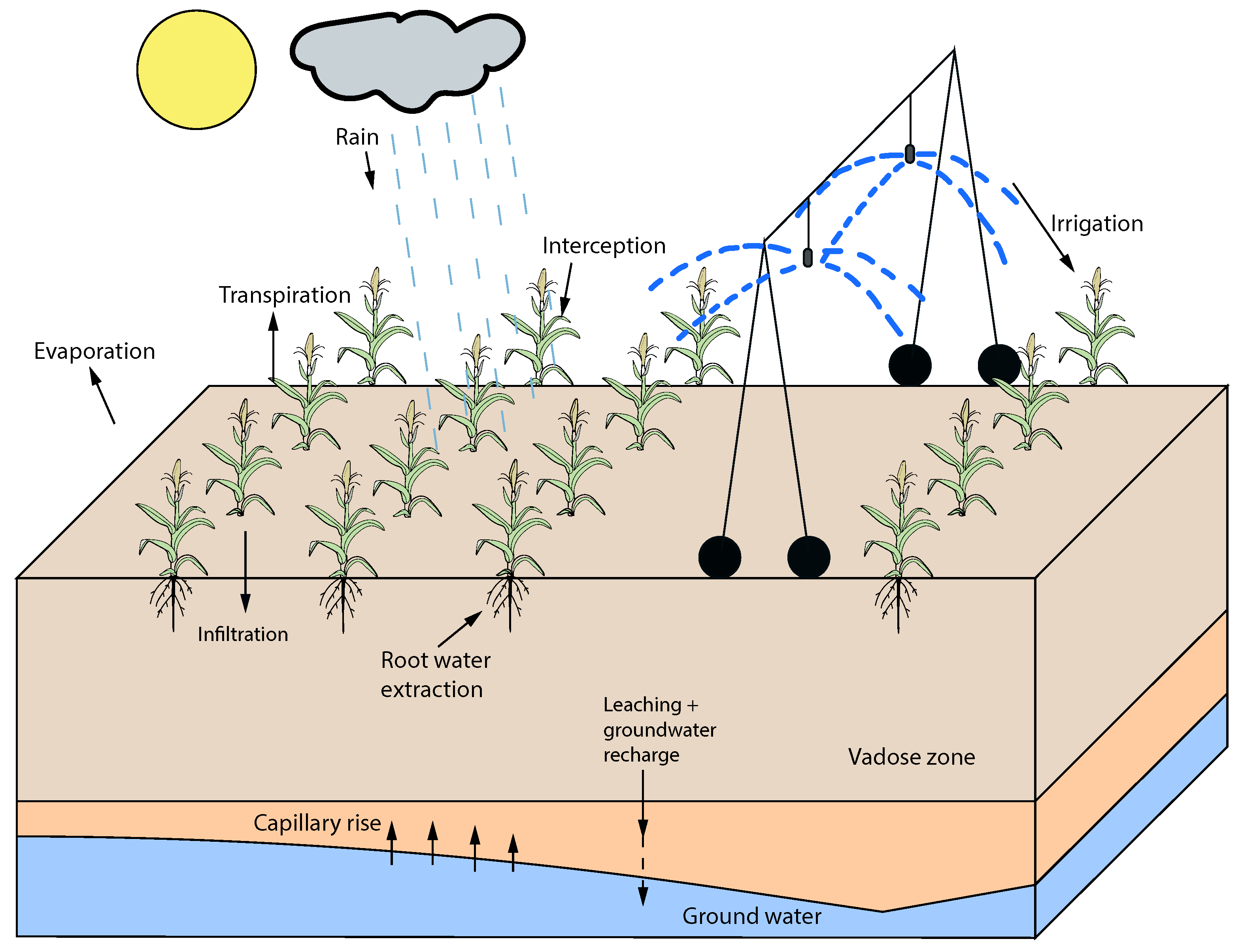
An agriculture field may have complex terrains, such as hill, valley, etc. It may contain more than one types of soil at different locations, for example, loam, clay, sand, etc. In order to capture the water dynamics of a field with multiple soil profiles, it is essential to introduce the 3D agro-hydrological system. In this work, we consider a simplified field with multiple types of soil with the following assumptions. First, the soil heterogeneity only presents in horizontal direction and the interface between two types of soil is vertical and flat. In other words, we assume that there is no mixture of different types of soil in the system. Second, for each type of soil, the irrigation is uniformly applied on the top surface. If the surface of one type of soil is significantly large and the irrigation equipment cannot cover the whole surface at the same time, this soil can be decomposed into sections with each section has the uniform irrigation/input. Third, the surface of the field is assumed to be flat, therefore, the effect of terrains is not studied in this work. A schematic of the 3D agro-hydrological system is shown in Figure 1, which is a modified version from [10]. In particular, we focus on the infiltration process in this work; that is, the water dynamics within the vadose zone of the soil. The water dynamics in the vadose zone of such a 3D field can be described using the following Richards’ equation:

$$c\left(h\right)\frac{\partial h}{\partial t}={\nabla }·\left[K\left(h\right){\nabla }\left(h+z\right)\right],$$

(1)

where h$\left(m\right)$ represents the capillary potential in the unsaturated soil, $K\left(h\right)$$(m/s)$ and $c\left(h\right)$$(1/m)$ are respectively the hydraulic conductivity and capillary capacity of the soil. The van Genuchten-Mualem soil hydraulic model $K\left(h\right)$ and $c\left(h\right)$ are utilized and shown in Equations (2) and (3), respectively [31]:

$$K\left(h\right)=K_s{\left[{\left(1+{\left(-\alpha h\right)}^n\right)}^{-\left(1-\frac{1}{n}\right)}\right]}^{\frac{1}{2}}{\left[1-{\left[1-{\left[{\left(1+{\left(-\alpha h\right)}^n\right)}^{-\left(1-\frac{1}{n}\right)}\right]}^{\frac{n}{n-1}}\right]}^{1-\frac{1}{n}}\right]}^2$$

(2)

$$c\left(h\right)=\left({\theta }_s-{\theta }_r\right)\alpha n\left(1-\frac{1}{n}\right){\left(-\alpha h\right)}^{n-1}{\left[1+{\left(-\alpha h\right)}^n\right]}^{-\left(2-\frac{1}{n}\right)},$$

(3)

where $K_s$ (m/s), ${\theta }_s$ (m${}^3$/m${}^3$) and ${\theta }_r$ (m${}^3$/m${}^3$) denote respectively the saturated hydraulic conductivity, the saturated soil moisture and the residual soil moisture of the considered soil, and $\alpha$ (1/m) and n are two more parameters that characterize the properties of the soil. For one type of soil, the parameter set ($K_s$, ${\theta }_s$, ${\theta }_r$, $\alpha$ and n) determines the properties of the soil. When more than one types of soil are considered, for each type of soil, it has its own set of parameters. Note that in the Richards’ Equation (1), the term z on the right-hand-side denotes the impact of gravitational force on water in the vertical $\left(z\right)$ direction and the vector differential operator (∇) in the 3D form summarizes the second derivatives of total pressure head with respect to x, y and z directions.

2.2. Model Discretization

The Richards’ equation in (1) is a nonlinear partial differential equation and is very difficult to solve analytically if ever possible. In order to find numerical approximations fo the solution of (1), we discretize the model using the finite difference (FD) method. The procedure to construct the FD model is detailed below.

First, the vector differential operation (∇) along the three spatial directions (x, y, z) is represented as the following:

$${\nabla }=\left[\frac{\partial }{\partial x}\frac{\partial }{\partial y}\frac{\partial }{\partial z}\right].$$

(4)

It is applied on Richards’ equation in (1), which results in the following form:

$$c\left(h\right)\frac{\partial h}{\partial t}=\frac{\partial }{\partial x}\left(K\left(h\right)\frac{\partial h}{\partial x}\right)+\frac{\partial }{\partial y}\left(K\left(h\right)\frac{\partial h}{\partial y}\right)+\frac{\partial }{\partial z}\left[K\left(h\right)\left(\frac{\partial h}{\partial z}+1\right)\right],$$

(5)

where the right-hand side is a summation of three terms, which are the second order derivatives of the total pressure head in x, y, and z directions, respectively. The first and second terms govern the water movements in x and y directions, respectively. Because the gravity force only applies to the water movement in the vertical (z) direction, $+1$ term does not present in the first and second terms.

Next, two-point central difference scheme and two-point forward difference scheme are used to approximate the derivatives with respect to spatial and temporal domains, respectively. Equations (6)–(8) below show the approximations of the derivative terms with respect to x, y, and z. Equation (9) illustrates how the derivative with respect to time is approximated.

$$\begin{array}{cc}\hfill {\left.\frac{\partial }{\partial x}\left(K\left(h\left(t\right)\right)\frac{\partial h\left(t\right)}{\partial x}\right)\right|}_{i,j,k}=& \frac{1}{{\Delta }{x}_i}\left[K_{i-\frac{1}{2},j,k}\left(h\left(t\right)\right)\left(\frac{h_{i-1,j,k}\left(t\right)-h_{i,j,k}\left(t\right)}{\frac{1}{2}({\Delta }{x}_{i-1}+{\Delta }{x}_i)}\right)\right.\hfill \\ & \left.-K_{i+\frac{1}{2},j,k}\left(h\left(t\right)\right)\left(\frac{h_{i,j,k}\left(t\right)-h_{i+1,j,k}\left(t\right)}{\frac{1}{2}({\Delta }{x}_i+{\Delta }{x}_{i+1})}\right)\right]\hfill \end{array}$$

(6)

$$\begin{array}{cc}\hfill {\left.\frac{\partial }{\partial y}\left(K\left(h\left(t\right)\right)\frac{\partial h\left(t\right)}{\partial y}\right)\right|}_{i,j,k}=& \frac{1}{{\Delta }{y}_j}\left[K_{i,j-\frac{1}{2},k}\left(h\left(t\right)\right)\left(\frac{h_{i,j-1,k}\left(t\right)-h_{i,j,k}\left(t\right)}{\frac{1}{2}({\Delta }{y}_{j-1}+{\Delta }{y}_j)}\right)\right.\hfill \\ & \left.-K_{i,j+\frac{1}{2},k}\left(h\left(t\right)\right)\left(\frac{h_{i,j,k}\left(t\right)-h_{i,j+1,k}\left(t\right)}{\frac{1}{2}({\Delta }{y}_j+{\Delta }{y}_{j+1})}\right)\right]\hfill \end{array}$$

(7)

$$\begin{array}{cc}\hfill {\left.\frac{\partial }{\partial z}\left[K\left(h\left(t\right)\right)\left(\frac{\partial h\left(t\right)}{\partial z}+1\right)\right]\right|}_{i,j,k}=& \frac{1}{{\Delta }{z}_k}\left[K_{i,j,k-\frac{1}{2}}\left(h\left(t\right)\right)\left(\frac{h_{i,j,k-1}\left(t\right)-h_{i,j,k}\left(t\right)}{\frac{1}{2}({\Delta }{z}_{k-1}+{\Delta }{z}_k)}+1\right)\right.\hfill \\ & \left.-K_{i,j,k+\frac{1}{2}}\left(h\left(t\right)\right)\left(\frac{h_{i,j,k}\left(t\right)-h_{i,j,k+1}\left(t\right)}{\frac{1}{2}({\Delta }{z}_k+{\Delta }{z}_{k+1})}+1\right)\right]\hfill \end{array}$$

(8)

$${\left.\frac{\partial h\left(t\right)}{\partial t}\right|}_{i,j,k}=\frac{h_{i,j,k}\left(t+1\right)-h_{i,j,k}\left(t\right)}{{\Delta }t}.$$

(9)

Note that in Equations (6)–(9), $i,j,k$ denote the locations of the discretized x, y, z directions, respectively, and t indicates the discrete time. Specifically, $i\in [1,N_{x,x}]\subset \mathbb{Z}$, $j\in [1,N_{x,y}]\subset \mathbb{Z}$, and $k\in [1,N_{x,z}]\subset \mathbb{Z}$, where $N_{x,x}$, $N_{x,y}$, and $N_{x,z}$ denote the number of compartments (or nodes) in x, y, and z directions. $t\in [0,N_t]\subset \mathbb{Z}$ where $N_t$ denotes the number of time instants considered. ${\Delta }t$ denotes the temporal step size. ${\Delta }{x}_i$, ${\Delta }{y}_j$, and ${\Delta }{z}_k$ represent the length (x direction), width (y direction), and depth (z direction) of the corresponding compartment, respectively.

The FD model that calculates the capillary pressure head at the position $i,j,k$ and the time instant $t+1$, is obtained by substituting Equations (6)–(9) into Equation (5) as shown below:

$$\begin{array}{cc}\hfill h_{i,j,k}(t+1)& =h_{i,j,k}\left(t\right)+\frac{{\Delta }t}{c_{i,j,k}\left(h\left(t\right)\right)}\{\frac{1}{{\Delta }{x}_i}\left[K_{i-\frac{1}{2},j,k}\left(h\left(t\right)\right)\left(\frac{h_{i-1,j,k}\left(t\right)-h_{i,j,k}\left(t\right)}{\frac{1}{2}({\Delta }{x}_{i-1}+{\Delta }{x}_i)}\right)\right.\hfill \\ \hfill & \left.-K_{i+\frac{1}{2},j,k}\left(h\left(t\right)\right)\left(\frac{h_{i,j,k}\left(t\right)-h_{i+1,j,k}\left(t\right)}{\frac{1}{2}({\Delta }{x}_i+{\Delta }{x}_{i+1})}\right)\right]+\frac{1}{{\Delta }{y}_j}\left[K_{i,j-\frac{1}{2},k}\left(h\left(t\right)\right)\left(\frac{h_{i,j-1,k}\left(t\right)-h_{i,j,k}\left(t\right)}{\frac{1}{2}({\Delta }{y}_{j-1}+{\Delta }{y}_j)}\right)\right.\hfill \\ \hfill & \left.-K_{i,j+\frac{1}{2},k}\left(h\left(t\right)\right)\left(\frac{h_{i,j,k}\left(t\right)-h_{i,j+1,k}\left(t\right)}{\frac{1}{2}({\Delta }{y}_j+{\Delta }{y}_{j+1})}\right)\right]+\frac{1}{{\Delta }{z}_k}\left[K_{i,j,k-\frac{1}{2}}\left(h\left(t\right)\right)\left(\frac{h_{i,j,k-1}\left(t\right)-h_{i,j,k}\left(t\right)}{\frac{1}{2}({\Delta }{z}_{k-1}+{\Delta }{z}_k)}+1\right)\right.\hfill \\ \hfill & \left.-K_{i,j,k+\frac{1}{2}}\left(h\left(t\right)\right)\left(\frac{h_{i,j,k}\left(t\right)-h_{i,j,k+1}\left(t\right)}{\frac{1}{2}({\Delta }{z}_k+{\Delta }{z}_{k+1})}+1\right)\right]\},\hfill \end{array}$$

(10)

where $c_{i,j,k}\left(h\right)=c\left(h_{i,j,k}\right)$ and the hydraulic conductivity is explicitly linearized as follows:

$$K_{i-\frac{1}{2},j,k}\left(h\right)=K\left(\frac{h_{i-1,j,k}+h_{i,j,k}}{2}\right),K_{i,j-\frac{1}{2},k}\left(h\right)=K\left(\frac{h_{i,j-1,k}+h_{i,j,k}}{2}\right),K_{i,j,k-\frac{1}{2}}\left(h\right)=K\left(\frac{h_{i,j,k-1}+h_{i,j,k}}{2}\right).$$

The Neumann boundary conditions are used to characterize the top, bottom, left, right, front, and back boundaries, which are shown below:

$$\begin{array}{ccccc}\hfill {\left.\frac{\partial h\left(t\right)}{\partial z}\right|}_{i,j,0}=& -1-\frac{q_{i,j,0}\left(t\right)}{K\left(h\left(t\right)\right)},\hfill & \hfill {\left.\frac{\partial h\left(t\right)}{\partial z}\right|}_{i,j,(N_{x,z}+1)}& =\hfill & \hfill -1-\frac{q_{i,j,(N_{x,z}+1)}\left(t\right)}{K\left(h\left(t\right)\right)}\\ \hfill {\left.\frac{\partial h\left(t\right)}{\partial x}\right|}_{0,j,k}=& -\frac{q_{0,j,k}\left(t\right)}{K\left(h\left(t\right)\right)},\hfill & \hfill {\left.\frac{\partial h\left(t\right)}{\partial x}\right|}_{(N_{x,x}+1),j,k}& =\hfill & \hfill -\frac{q_{(N_{x,x}+1),j,k}\left(t\right)}{K\left(h\left(t\right)\right)}\\ \hfill {\left.\frac{\partial h\left(t\right)}{\partial y}\right|}_{i,0,k}=& -\frac{q_{i,0,k}\left(t\right)}{K\left(h\left(t\right)\right)},\hfill & \hfill {\left.\frac{\partial h\left(t\right)}{\partial y}\right|}_{i,(N_{x,y}+1),k}& =\hfill & \hfill -\frac{q_{i,(N_{x,y}+1),k}\left(t\right)}{K\left(h\left(t\right)\right)}.\end{array}$$

(11)

In the above equations, if either of i, j or k equals to zero, it means the boundary is either of left, front or top boundary, respectively. On the other hand, if it equals to either of $N_{x,x}+1$, $N_{x,y}+1$ or $N_{x,z}+1$, the boundary is either of right, back, or bottom boundary. The variable q ($m/s$) denotes the water flow rate. In particular, $q_{i,j,0}$ represents the irrigation rate supplied at the surface point $i,j$. It is considered as the input of the system. By following the standard 3D Cartesian coordinate system, when the water flows in the same direction of one of positive axes, the flow rate is defined as a positive value. On the contrary, the flow rate has a negative value when the water flows in the opposite direction. The incorporation of flux based boundary conditions into the Richards’ equation is shown below with top boundary as an example.

By rearranging the 1st boundary condition in Equation (11), the irrigation rate can be represented as the following:

$$-q_{i,j,0}\left(t\right)=K\left(h\left(t\right)\right)\left({\left.\frac{\partial h\left(t\right)}{\partial z}\right|}_{i,j,0}+1\right).$$

(12)

Since only unsaturated case is considered in this work, it is not necessary to calculate the value of the capillary pressure head at the top boundary ($h_{i,j,0}$), when calculating the capillary pressure head at the top layer ($h_{i,j,1}$). Instead, the term $K_{i,j,\frac{1}{2}}\left(h\left(t\right)\right)\left(\frac{h_{i,j,0}\left(t\right)-h_{i,j,1}\left(t\right)}{{\Delta }{z}_0}+1\right)$ in Equation (10) can be substituted by Equation (12). Then $h_{i,j,1}$ is calculated by directly using the irrigation rate, $q_{i,j,0}$, instead of $h_{i,j,0}$.

2.3. Augmented Model

A compact form describing the 3D infiltration process can be obtained by combining Equations (10)–(12) of all the spatial discretization nodes and adding in process and measurement noise terms, which is represented as below:

$$\begin{array}{cc}\hfill x(t+1)& =F(x\left(t\right),u\left(t\right),p\left(t\right))+{\omega }_x\left(t\right)\hfill \\ \hfill y\left(t\right)& =Cx\left(t\right)+\nu \left(t\right),\hfill \end{array}$$

(13)

where $x\left(t\right)\subset {\mathbb{R}}^{N_x}$ is the state vector which is a collection of all the capillary pressure heads ($h_{i,j,k}$ in (10)) at each discretization point, $u\left(t\right)\subset {\mathbb{R}}^{N_u}$ is the input vector (a collection of irrigation rates at all the nodes of the top surface), $p\left(t\right)\subset {\mathbb{R}}^{N_p}$ denotes the parameter vector, ${\omega }_x\left(t\right)\subset {\mathbb{R}}^{N_{{\omega }_x}}$ represents the system noise, $y\left(t\right)\subset {\mathbb{R}}^{N_y}$ is the system output vector, and $\nu \left(t\right)\subset {\mathbb{R}}^{N_{\nu }}$ denotes the measurement noise. The state is the capillary pressure head and the total number ($N_x$) of the states is the product of $N_{x,x}$, $N_{x,y}$ and $N_{x,z}$. The size of the parameter vector ($N_p$) depends on the number of types of soil presented in the system. The output is obtained by directly measuring some of the states.

In order to estimate the states and parameters simultaneously, the parameters are augmented as extra system states assuming that the parameters are constant as follows:

$$p\left(k+1\right)=p\left(k\right).$$

(14)

The augmented process model is shown below:

$$\begin{array}{cc}\hfill x_a(t+1)& =F_a(x_a\left(t\right),u\left(t\right))+{\omega }_a\left(t\right)\hfill \\ \hfill y\left(t\right)& =C_a{x}_a\left(t\right)+\nu \left(t\right),\hfill \end{array}$$

(15)

where the subscript a denotes the augmentation, $x_a\left(t\right)\subset {\mathbb{R}}^{N_{x_a}}$ is the augmented state vector, which is $x_a={[x,p]}^T$. The augmented process noise is denoted as ${\omega }_a\left(t\right)\subset {\mathbb{R}}^{N_{w_a}}$.

3. Proposed Estimation Method

In our previous work [10], it was found that MHE outperforms EKF and EnKF due to its ability in handling constraints. In this work, we will adopt MHE as the estimation algorithm as well. We consider fields with more than one types of soil and propose to use decentralized MHE for simultaneously state and parameter estimation. In this section, we will first present the guidelines for subsystem decomposition in Section 3.1, then discuss how to use observability analysis and sensitivity analysis to pick the set of parameters for estimation. Following this, we will show why a decentralized framework is appropriate in Section 3.3. At last, Section 3.4 presents the proposed DeMHE design.

3.1. Guidelines for Subsystem Decomposition

In the development of a decentralized estimation scheme, the first step is to decompose the entire process into smaller subsystems. For a 3D infiltration system, we propose the following guidelines for subsystem decomposition:

• it is expected that the numbers of the states in the configured subsystems can be made similar, such that the computational and organizational complexity of the local estimators are not significantly different;
• it is desirable if each subsystem only accounts for one soil type;
• it is expected that the initial values of the states involved in each subsystem are relatively similar;
• it is expected that the areas that are subject to different irrigation schedules are assigned to different subsystems;
• it is expected that each configured subsystem is assigned sufficient sensors such that the subsystem is observable;
• it is important that the dynamical interaction between each two subsystems is made minimal.

Following the guidelines, each subsystem represents a relatively small 3D field, which contains only one type of soil and its irrigation is uniformly applied.

3.2. Significant Parameter Selection and Minimal Number of Sensors

Before conducting subsystem decomposition, it is necessary to conduct an observability test of the centralized augmented system of Equation (15) to ensure that the system is observable assuming that all the pressure head states are measured [10,16]. Based on the observability results, if the system of Equation (15) is not observable, it is essential to remove some of the parameters from the augmented system. This can be achieved by finding the most significant parameters that can ensure the observability of the augmented system. The significant parameter subset for estimation may be selected using sensitivity analysis. Once the significant parameters are identified, we can determine the the minimum number of sensors required to ensure the observability of the system using the maximum multiplicity method [32]. The detailed algorithms for testing the observability, finding the significant parameter subset and determining the minimal number of sensors are discussed in [10]. The application of these algorithms to a 3D infiltration process will be discussed in the simulations.

3.3. Subsystem Approximation and Motivation of Decentralized Estimation

It is favorable to use a 3D Richards’ equation to develop the state and parameter estimation algorithm. However, a 3D model with fine discretization leads to increased number of states, which MHE may not be able to handle in an online fashion. One of the benefits of the proposed subsystem guidelines is that the states on a horizontal layer within a subsystem are very similar. Therefore, it is possible to use, for example, the states at the center column (a 1D system) of a subsystem to approximate the vertical capillary potential dynamics of different nodes within the same subsystem. Based on this, we further propose to use a 1D Richards’ equation to approximate the dynamics of each 3D subsystem. This can significantly reduce the computational demand for each decentralized estimator. Specifically, we propose to use the center column of each subsystem to approximate the vertical water dynamcis of a subsystem.

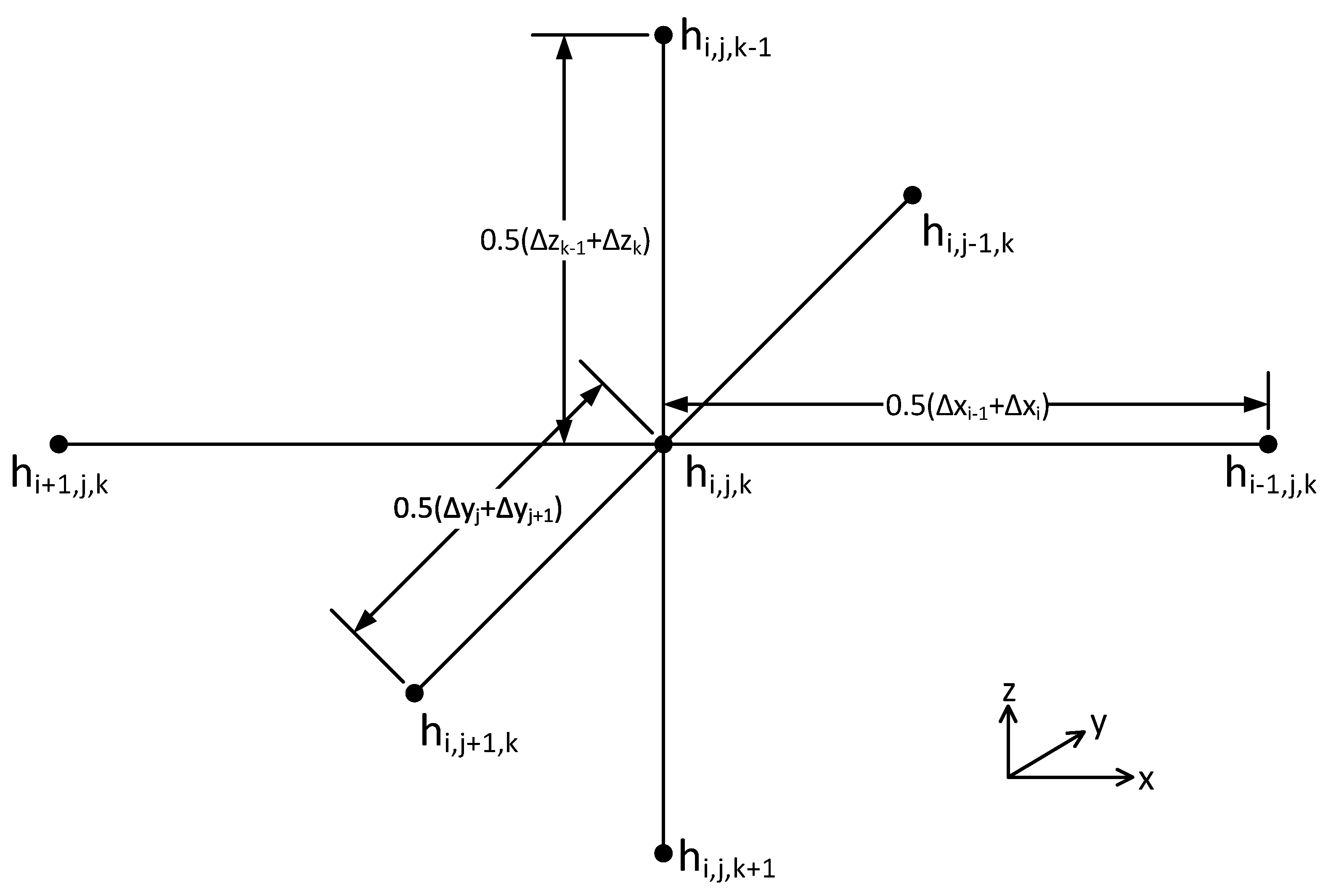
Based on this approximation, we study the significance of interaction between subsystems and motivate the use of a decentralized estimation framework. First, according to the FD model of Equation (10), the state at time instant $t+1$, $h_{i,j,k}(t+1)$ is dependent on itself and its adjacent states at time instant t. Figure 2 shows an illustration of the neighboring states of $h_{i,j,k}$. Let us assume that the states $h_{i,j,k}$, $h_{i,j,k-1}$ and $h_{i,j,k+1}$ belong to (a 1D approximation of) one subsystem, and $h_{i-1,j,k}$, $h_{i+1,j,k}$, $h_{i,j-1,k}$ and $h_{i,j+1,k}$ belong to the neighbouring subsystems. Let us examine the following term on the right-hand side of Equation (10):

$$\frac{1}{{\Delta }{x}_i}\left[K_{i-\frac{1}{2},j,k}\left(h\left(t\right)\right)\left(\frac{h_{i-1,j,k}\left(t\right)-h_{i,j,k}\left(t\right)}{\frac{1}{2}({\Delta }{x}_{i-1}+{\Delta }{x}_i)}\right)-K_{i+\frac{1}{2},j,k}\left(h\left(t\right)\right)\left(\frac{h_{i,j,k}\left(t\right)-h_{i+1,j,k}\left(t\right)}{\frac{1}{2}({\Delta }{x}_i+{\Delta }{x}_{i+1})}\right)\right].$$

Suppose that the discretization along x direction is equally spaced, the above term can be further simplified into the following:

$$\frac{K_{i-\frac{1}{2},j,k}\left(h\left(t\right)\right)\left[h_{i-1,j,k}\left(t\right)-h_{i,j,k}\left(t\right)\right]-K_{i+\frac{1}{2},j,k}\left(h\left(t\right)\right)\left[h_{i,j,k}\left(t\right)-h_{i+1,j,k}\left(t\right)\right]}{{\left({\Delta }x\right)}^2}.$$

(16)

This term quantitatively measures how the neighboring states along x direction ($h_{i-1,j,k}$ and $h_{i+1,j,k}$) contribute to the evolution of $h_{i,j,k}$. Similarly, the following two terms quantify how neighboring states in y and z directions affect the evolution of $h_{i,j,k}$, respectively:

$$\frac{K_{i,j-\frac{1}{2},k}\left(h\left(t\right)\right)\left[h_{i,j-1,k}\left(t\right)-h_{i,j,k}\left(t\right)\right]-K_{i,j+\frac{1}{2},k}\left(h\left(t\right)\right)\left[h_{i,j,k}\left(t\right)-h_{i,j+1,k}\left(t\right)\right]}{{\left({\Delta }y\right)}^2}$$

(17)

$$\frac{K_{i,j,k-\frac{1}{2}}\left(h\left(t\right)\right)\left[h_{i,j,k-1}\left(t\right)-h_{i,j,k}\left(t\right)+1\right]-K_{i,j,k+\frac{1}{2}}\left(h\left(t\right)\right)\left[h_{i,j,k}\left(t\right)-h_{i,j,k+1}\left(t\right)+1\right]}{{\left({\Delta }z\right)}^2}.$$

(18)

According to Equation (10), the summation of the above three terms contributes to the evolution of $h_{i,j,k}$. As mentioned before, ${\Delta }x$ and ${\Delta }y$ represent the horizontal distances between two subsystems. Their values can be a few meters or even larger. ${\Delta }z$ is the interval beween two vertical discretization nodes and its value typically is about 1 to 25 centimeters. For example, if ${\Delta }x={\Delta }y=10m$ and ${\Delta }z=1cm$, then, the denominator of term (18) is ${10}^6$ times smaller than those of terms (16) and (17). Because the seven states shown in Figure 2 have values of similar magnitudes, the numerators of the above three terms are of similar magnitudes. Hence, the term (18) is around ${10}^6$ times greater than terms (16) and (17), which implies that the contribution of the states in z direction ($h_{i,j,k-1}$ and $h_{i,j,k+1}$) to the evolution of $h_{i,j,k}$ is significantly larger than those in x and y directions. In other words, the horizontal interaction between the states is notably smaller, as compared to the vertical interaction between the states. This justifies the use a decentralized estimation framework.

3.4. Decentralized Moving Horizon Estimation Design

In the proposed DeMHE design, a 1D model that approximates the corresponding 3D subsystem is used in the local MHE design. For subsystem n, its 1D approximation is described as follows:

$$\begin{array}{cc}\hfill x_a^n(t+1)& =F_a^n(x_a^n\left(t\right),u^n\left(t\right))+{\omega }_a^n\left(t\right)\hfill \\ \hfill y^n\left(t\right)& =C_a^n{x}_a^n\left(t\right)+{\nu }^n\left(t\right),\hfill \end{array}$$

(19)

where the superscript $n\in [1,N_s]\subset \mathbb{Z}$ denotes the index of the subsystem, $x_a^n\left(t\right)\subset {\mathbb{R}}^{N_{x_a^n}}$ is the state vector of the 1D approximation of subsystem n augmented with the to-be-estimated parameters of subsystem n, $y^n\left(t\right)\subset {\mathbb{R}}^{N_{y^n}}$ is the $n^{th}$ subsystem’s output vector, and ${\omega }_a^n\left(t\right)\subset {\mathbb{R}}^{N_{{\omega }_a^n}}$ and ${\nu }^n\left(t\right)\subset {\mathbb{R}}^{N_{{\nu }^n}}$ represent the subsystem’s process and measurement noise.

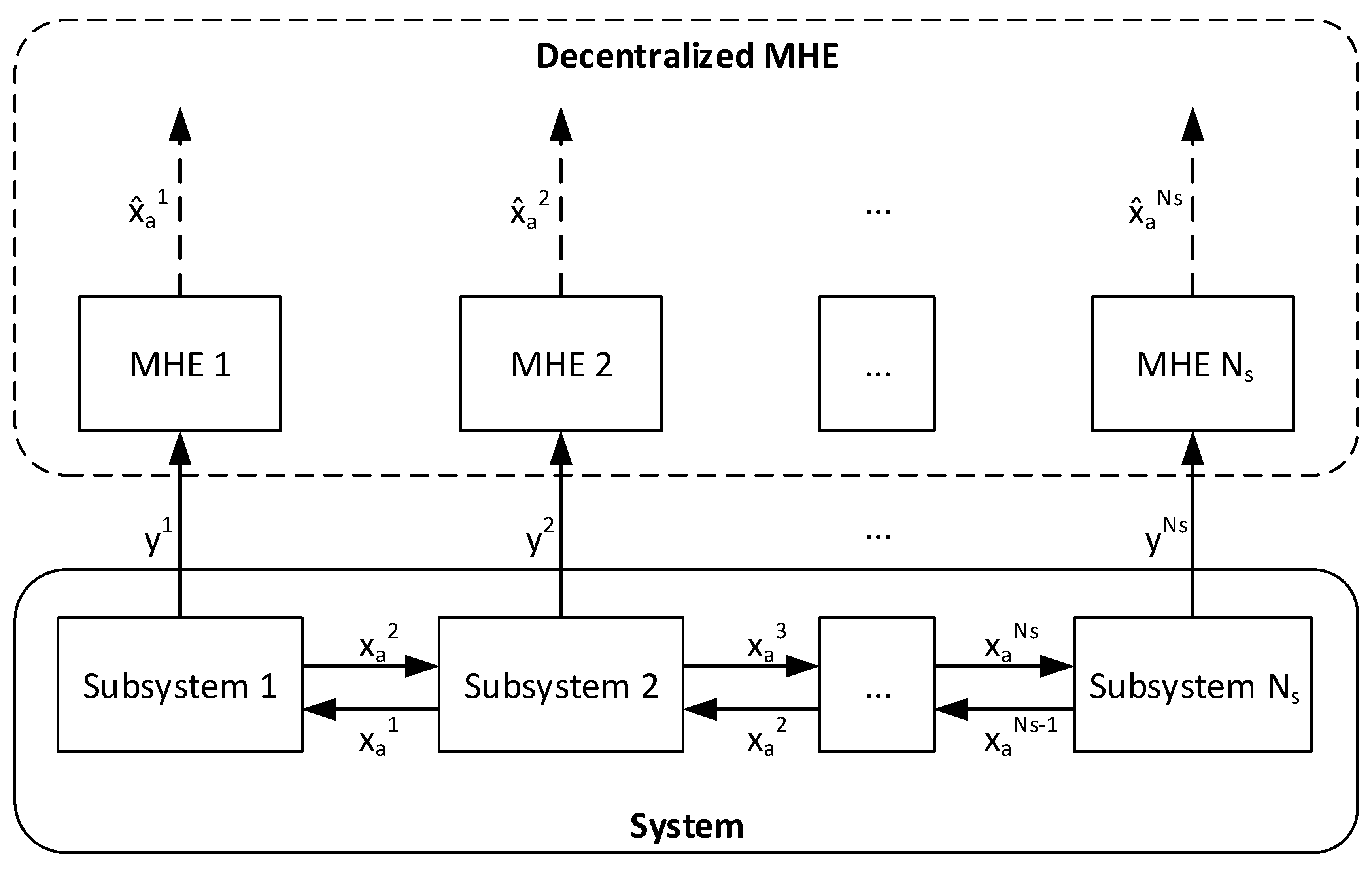
A schematic diagram of the proposed DeMHE is shown in Figure 3. At every sampling time, the measurements from the subsystems are measured and sent to the corresponding estimators. The estimator will only utilize the measurements from the corresponding subsystem and not from other subsystems. Each estimator is independent on each other in the proposed DeMHE. In each local estimator, the 1D approximation of the subsystem is used. The mathematical formulation of the MHE design of subsystem n is shown below:

$$\underset{\begin{array}{c}{\hat{x}}_a^n(t-N^n),\cdots ,{\hat{x}}_a^n\left(t\right),\\ {\hat{\omega }}_a^n(t-N^n),\cdots ,{\hat{\omega }}_a^n(t-1)\end{array}}{min}\left\{\begin{array}{c}{\displaystyle {∥{\hat{x}}_a^n(t-N^n)-{\overline{x}}_a^n(t-N^n)∥}_{{\left(P^n\right)}^{-1}}^2+\sum _{l=t-N^n}^{t-1}{∥{\hat{\omega }}_a^n\left(l\right)∥}_{{\left(Q^n\right)}^{-1}}^2}\\ {\displaystyle +\sum _{l=t-N^n}^t{∥{\hat{\nu }}^n\left(l\right)∥}_{{\left(R^n\right)}^{-1}}^2}\end{array}\right\}$$

(20)

$$\mathrm{s}.\mathrm{t}.{\hat{x}}_a^n(l+1)=F_a^n({\hat{x}}_a^n\left(l\right),u^n\left(l\right))+{\hat{\omega }}_a^n\left(l\right),l\in [t-N^n,t-1]\subset \mathbb{Z}$$

(21)

$${\hat{\nu }}^n\left(l\right)=y^n\left(l\right)-C_a^n{\hat{x}}_a^n\left(l\right),l\in [t-N^n,t]\subset \mathbb{Z}$$

(22)

$${\hat{x}}_a^n\left(l\right)\in {\mathbb{X}}_a^n,{\hat{\nu }}^n\left(l\right)\in {\mathbb{V}}^n,l\in [t-N^n,t]\subset \mathbb{Z}$$

(23)

$${\hat{\omega }}_a^n\left(l\right)\in {\mathbb{W}}_a^n,l\in [t-N^n,t-1]\subset \mathbb{Z}$$

(24)

where n denotes the index of the estimator, $N^n$ is the estimation window size of the estimator n, ${\hat{x}}_a^n$, ${\hat{\omega }}_a^n$, and ${\hat{\nu }}^n$ are the estimates of $x_a^n$, ${\omega }_a^n$, and ${\nu }^n$ within the estimation window. In the cost function (20), the matrices $P^n$, $Q^n$, and $R^n$ are the covariance matrices of the subsystem’s state uncertainty, model noise, and measurement noise. For different subsystems with different soil types, the design of the penalty matrices for each corresponding MHE could be different while the formulation of the MHE remains the same. In the design, (21) and (22) are the subsystem model. The constraints on the subsystem state, process and measurement noise are denoted as ${\mathbb{X}}_a^n$, ${\mathbb{W}}_a^n$, and ${\mathbb{V}}^n$, which are shown in Equations (23) and (24).

4. Simulation Results and Discussion

4.1. System Description

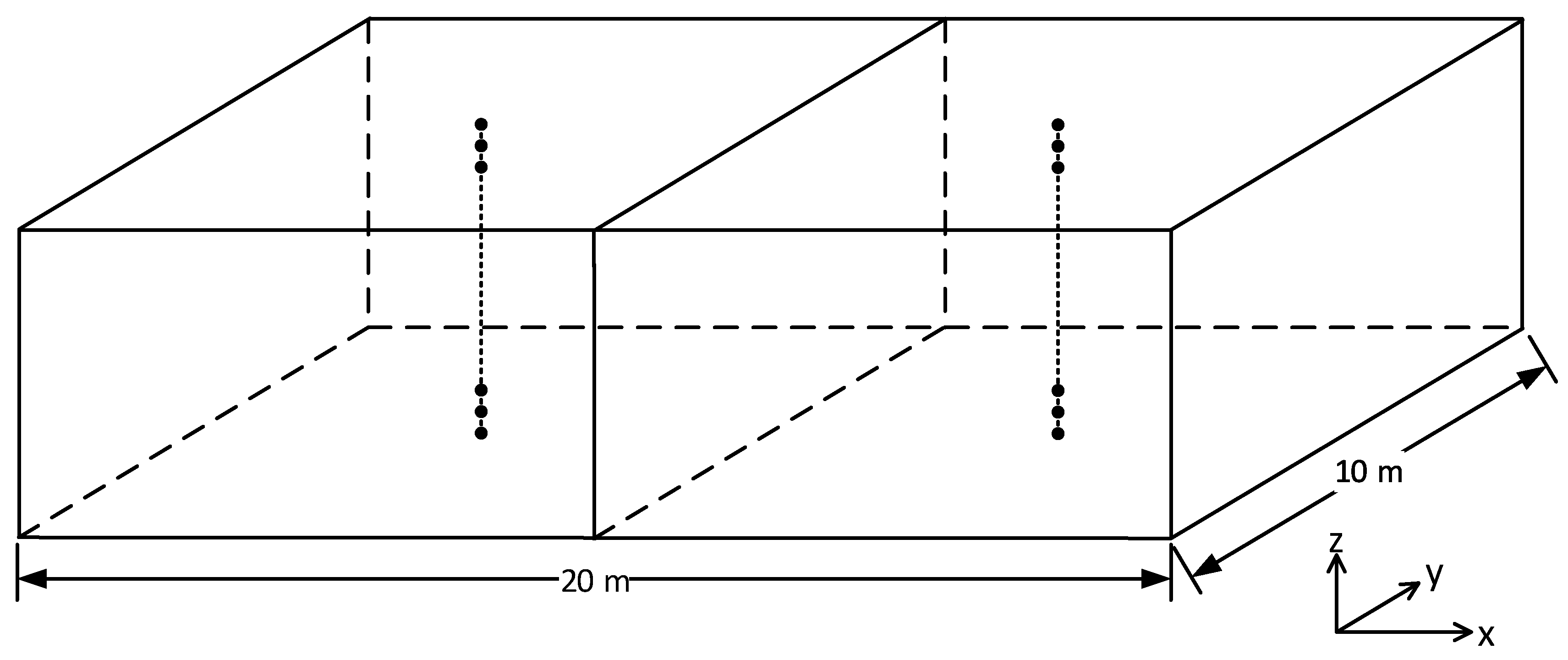
A field with 20 m ($L_x$) in x direction, 10 m ($L_y$) in y direction and a total depth ($L_z$) of 67 cm is investigated. A schematic of the field is shown in Figure 4. The soil type is loam on the left half of the field and is sandy clay loam (SCL) on the right half. The parameters of two types of soil are shown in

Table 1. The parameters of the investigated 3D field.

	${\mathit{K}}_{\mathit{s}}$ (m/s)	${\mathit{\theta }}_{\mathit{s}}$$({\mathbf{m}}^3/{\mathbf{m}}^3)$	${\mathit{\theta }}_{\mathit{r}}$$({\mathbf{m}}^3/{\mathbf{m}}^3)$	$\mathit{\alpha }$$(1/\mathbf{m})$	n
Loam	$2.89\times {10}^{-6}$	0.430	0.0780	3.60	1.56
Sandy clay loam	$3.64\times {10}^{-6}$	0.390	0.100	5.90	1.48

[33]. In the following simulations, the field is equally partitioned into 500 compartments in x direction ($N_{x,x}=500$), 250 compartments in y direction ($N_{x,y}=250$), and 32 compartments in z direction ($N_{x,z}=32$). Each discretization node (state) is centered at the corresponding compartment.

4.2. Observability Test on Original System

As described in Section 3.2, it is necessary to ensure the observability of the original system before performing decomposition, since the system contains two different types of soil, loam and sandy clay loam. There are in total 10 soil parameters (5 for each type of soil). Following the approach presented in [10], we determine the significant identifiable parameters, determine the minimum number of sensors required to ensure the identifiability of the parameters.

Initially, all the 10 parameters ($K_s$, ${\theta }_s$, ${\theta }_r$, $\alpha$, and n for loam and sandy clay loam) are augmented to the FD model of the field and all the states (soil moisture) are assumed to be measured. Based on the FD model of the field, a 4-day simulation is carried out under the following settings: (a) on the surface of the soil, the irrigation (u) is performed at the rate of 2.50 cm/day, from 12:00 PM to 4:00 PM daily; (b) at the bottom, the free drainage boundary condition is applied, and (c) the field has the homogeneous initial condition $\left(x\right(0\left)\right)$ of −0.514 m capillary pressure head. The generated data are used in the rest of the subsection. It is assumed that the measurements are available every hour.

Following the procedure discussed in [10], the PBH observability test is applied on the augmented system of Equation (15) to check the identifiability of the parameters. The system needs to be linearized every sampling time. It shows that the augmented system is not observable when all 10 parameters are augmented, even all the soil moisture states are measured. In order to look for an observable system, parameters are removed from the augmented system. It starts with removing only one of the parameters and this results in 10 different augmented systems with each one augmented with nine parameters. It is found that none of the systems are observable. Then, two parameters are removed from the system, which results in 45 different augmented systems. By checking their observability, it shows that there are four observable systems. The parameters removed from these four candidates are listed in

Table 2. Observable systems and their removed parameters.

Candidate #	Parameters Removed
1	${\theta }_s$ of loam and ${\theta }_s$ of SCL
2	${\theta }_r$ of loam and ${\theta }_r$ of SCL
3	${\theta }_s$ of loam and ${\theta }_r$ of SCL
4	${\theta }_r$ of loam and ${\theta }_s$ of SCL

. Since observable systems are found, the final parameter set is determined in the next step.

Sensitivity analysis described in [10] is conducted based on the original augmented system with all the parameters augmented. By comparing 1-norm of each column of the normalized sensitivity matrices $S_N$, it can be found that the 1-norm of the column $\frac{\partial y_i}{\partial {\theta }_s}$ of both loam (5050) and SCL (2.34) are bigger than 1-norm of $\frac{\partial y_i}{\partial {\theta }_r}$ of loam (916) and SCL (0.600), respectively. Based on this, ${\theta }_s$ of the two types of soil are considered as the more important parameters because they have more impacts on the output than ${\theta }_r$. It is worth mentioning that even the 1-norm of $\frac{\partial y_i}{\partial {\theta }_s}$ of SCL (2.34) is much smaller than 1-norm of $\frac{\partial y_i}{\partial {\theta }_r}$ of loam (916), ${\theta }_r$ of loam is neglected in estimation problem. The reason is that if both ${\theta }_s$ and ${\theta }_r$ of loam are augmented in the system, the system becomes unobservable. Therefore, the parameter set (Candidate 2) excluding both ${\theta }_r$ is selected and the final parameter set used in the remaining analysis is $\{K_s,{\theta }_s,\alpha ,n\}$ for both loam and sandy clay loam.

In the above, the identifiable and significant parameter set is determined based on the assumption that all states are measured. The minimum number of sensors (measurements) is determined, following the method described in [10] by using the maximum multiplicity method. It can be found that the minimum number of sensors is 8 to ensure the observability of the augmented system with 8 parameters.

4.3. Subsystem Decomposition

Following the guidelines for subsystem decomposition in Section 3.1, we can decompose the entire field into two subsystems. Subsystem 1 contains the loam on the left of the field and subsystem 2 contains the SCL on the right half of the field. Based on the discretization discussed in Section 4.1, each subsystem contains 2 million states representing the capillary potentials, 4 soil parameters to be augmented and estimated, and 4 measured outputs.

Because the soil property in each subsystem is homogeneous, initial state and input are uniform for each subsystem, it is reasonable to expect that the dynamics along x and y directions are minor and the dominant dynamics happens in the vertical direction. Therefore, it is reasonable to use the state at the center column of a subsystem to approximate the dynamics of the entire subsystem. Under this situation, each 3D subsystem can be approximated by a 1D model which contains only 32 states, 4 augmented parameters, 4 outputs and 1 input. In Figure 4, the column of black solid dots represents the states of the center column of each subsystem.

In order to ensure the above assumptions are valid, it is necessary to compare the numerical solutions of the original FD model and the 1D approximation of the two subsystems. In the original FD model, ${\Delta }x$ and ${\Delta }y$ both equal to 4 cm. We will refer to the original FD model as Model 1. In the scheme with 1D approximations of the two subsystems, we essentially have ${\Delta }x$ and ${\Delta }y$ both equal to 10 m. We will refer to this scheme as Model 2. Three scenarios are considered and the simulation settings are listed in

Table 3. Scenarios studying effects of sizes of ${\Delta }x$ and ${\Delta }y$ on numerical solution of the 3D Richards’ equation.

	$\mathit{x}\left(0\right)$$\left(\mathbf{m}\right)$		u$(\mathbf{cm}/\mathbf{day})$		Irrigation Schedule
Soil type	Loam	SCL	Loam	SCL	Loam	SCL
Scenario 1	−0.514	−0.514	2.5	2.5	12PM to 4PM	12PM to 4PM
Scenario 2	−0.514	−0.284	2.5	2.5	12PM to 4PM	12PM to 4PM
Scenario 3	−0.514	−0.514	2.5	2.5	12PM to 2PM	2PM to 4PM

. The numerical solutions of two models are compared in all three scenarios. Specifically, the setup of Scenario 1 is that at the surface of the soil, the irrigation (u) is performed at the rate of 2.50 cm/day, from 12:00 PM to 4:00 PM daily. At the bottom, the free drainage boundary condition is applied. The field has the homogeneous initial condition $\left(x\right(0\left)\right)$ of −0.514 m capillary pressure head. Scenario 2 studies the impact of initial conditions. The left half of the field has the homogeneous initial condition of −0.514 m capillary pressure head and the right half has the homogeneous initial condition of −0.284 m. The top and bottom boundary conditions of this scenario is the same as the setup of Scenario 1. Scenario 3 studies the impact of inputs on the numerical solution. It has the same initial condition and bottom boundary condition as Scenario 1. However, the irrigation is performed at the rate of 2.5 cm/day, from 12:00 PM to 2:00 PM daily on the left half of the field and from 2:00 PM to 4:00 PM daily on the right half.

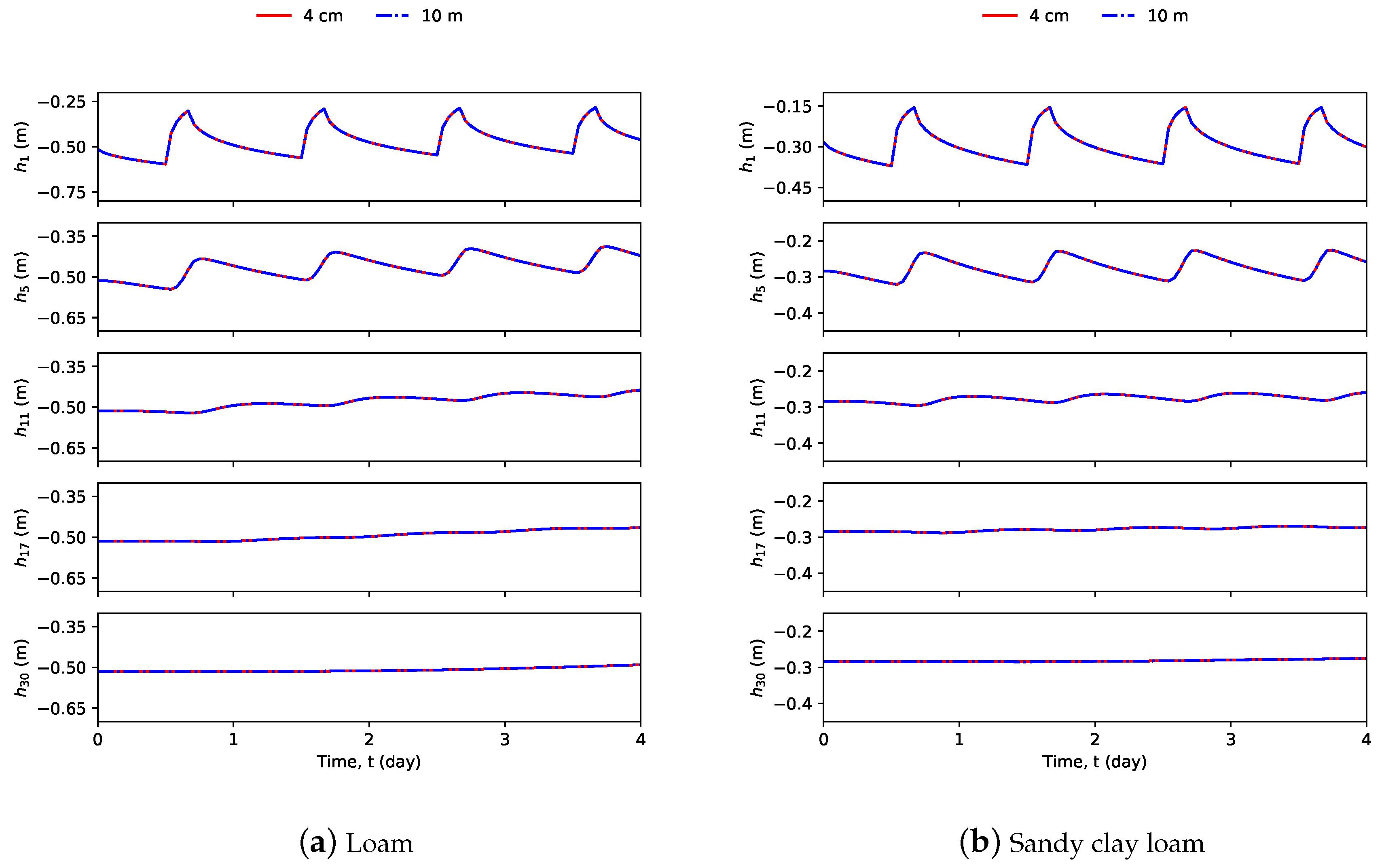
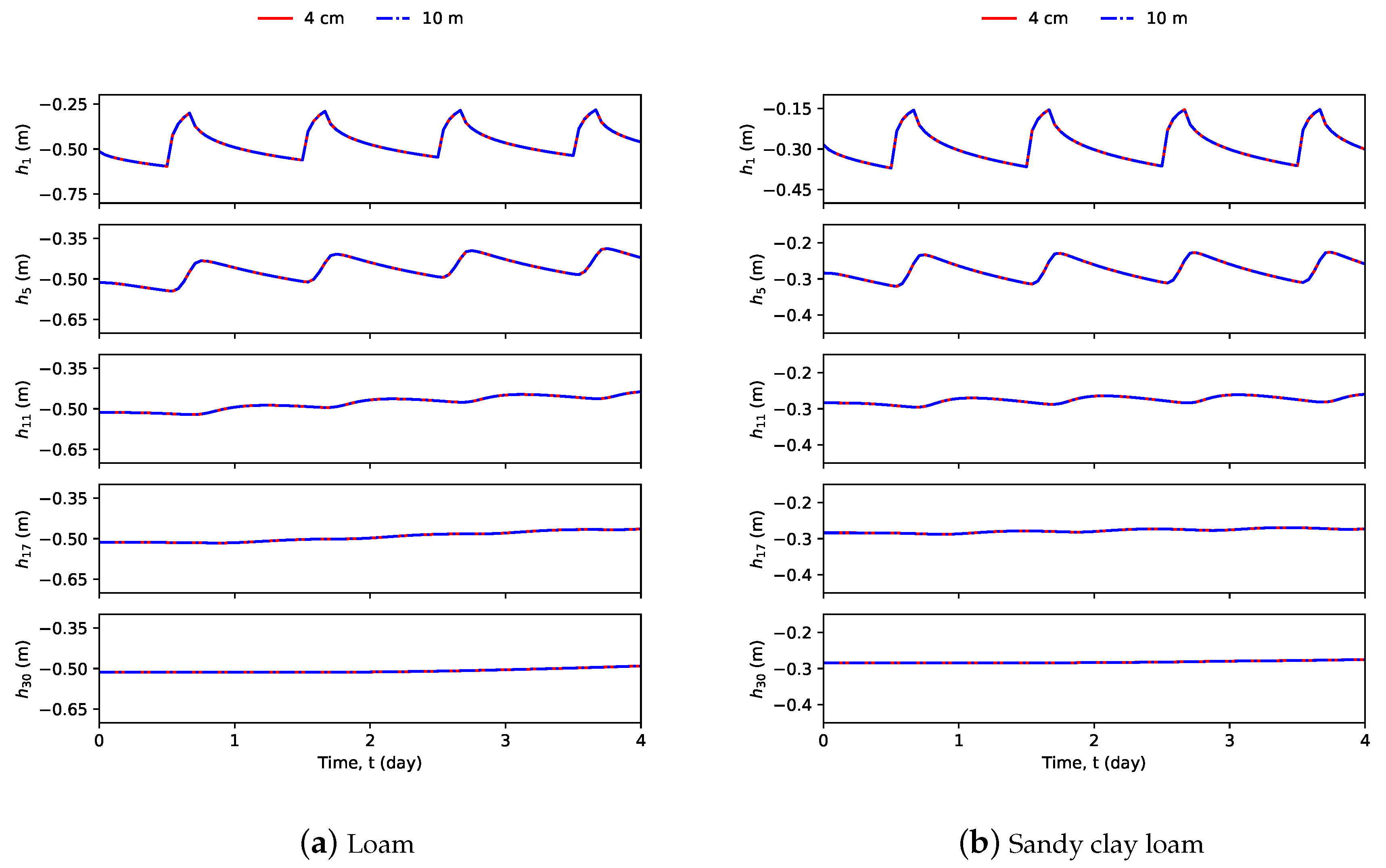
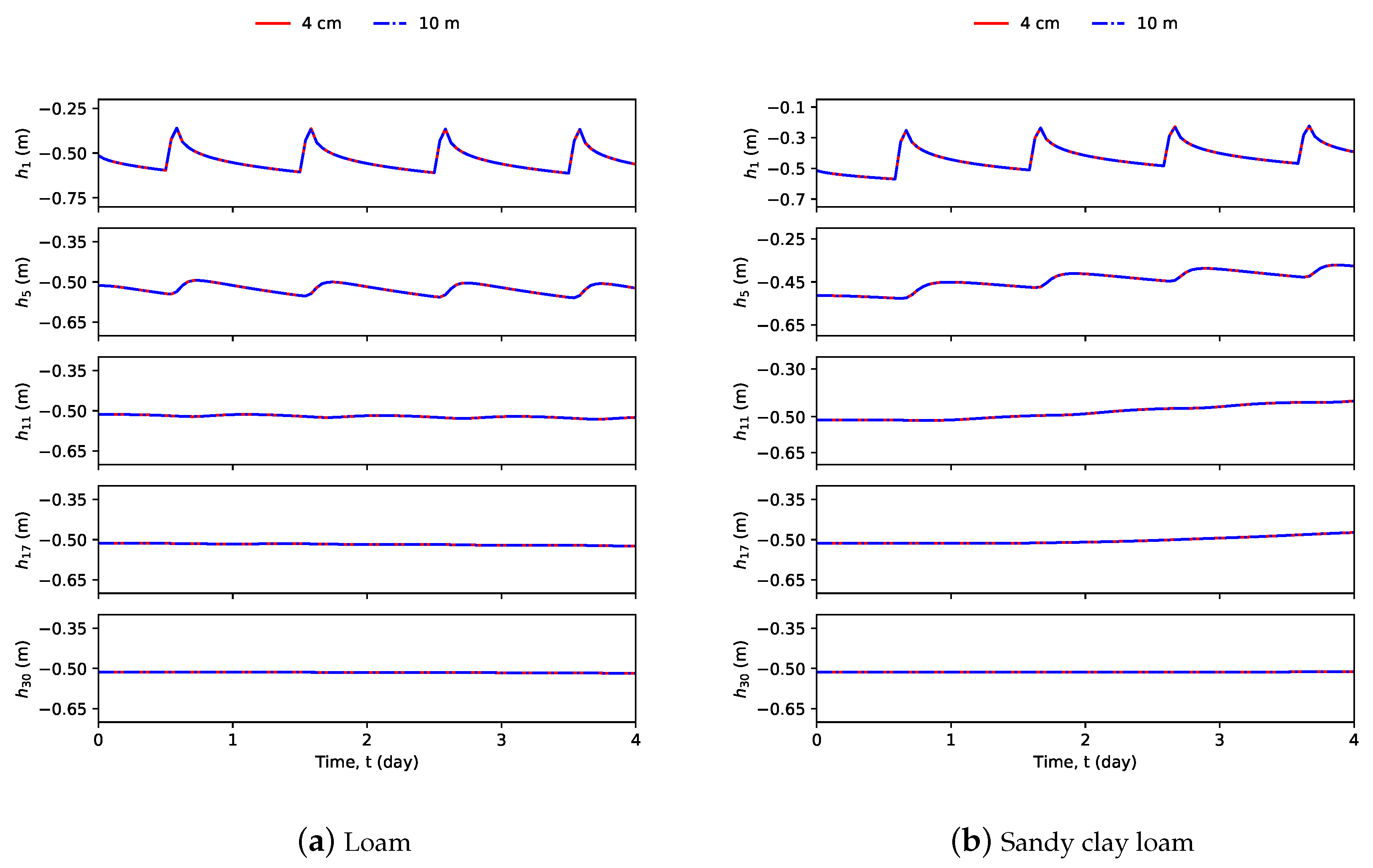
The three figures, Figure A1, Figure A2, and Figure A3 in Appendix A, show the selected state trajectories comparing two models under Scenario 1, 2, and 3, respectively. Within each figure, the subplot on the left shows the trajectories of the loam and the subplot on the right shows the trajectories of sandy clay loam. Under each scenario, the trajectories of Model 2 is almost the same as those of Model 1. Qualitatively speaking, the maximum percentage difference over the investigated time domain of Scenario 1, 2, and 3 is 0.01%, 0.03%, and 0.006%, respectively. This implies that Model 2 is a good approximation of the original FD model. In conclusion, for a subsystem that contains only 1 type of soil, receives uniform irrigation and is initialized uniformly, the capillary potential at the center of the subsystem (black dots) is able to represent the capillary potentials at other locations in the same horizontal layer. Hence, it is reasonable to only use an 1D model to simulate the subsystem.

4.4. Simultaneous Parameter and State Estimation

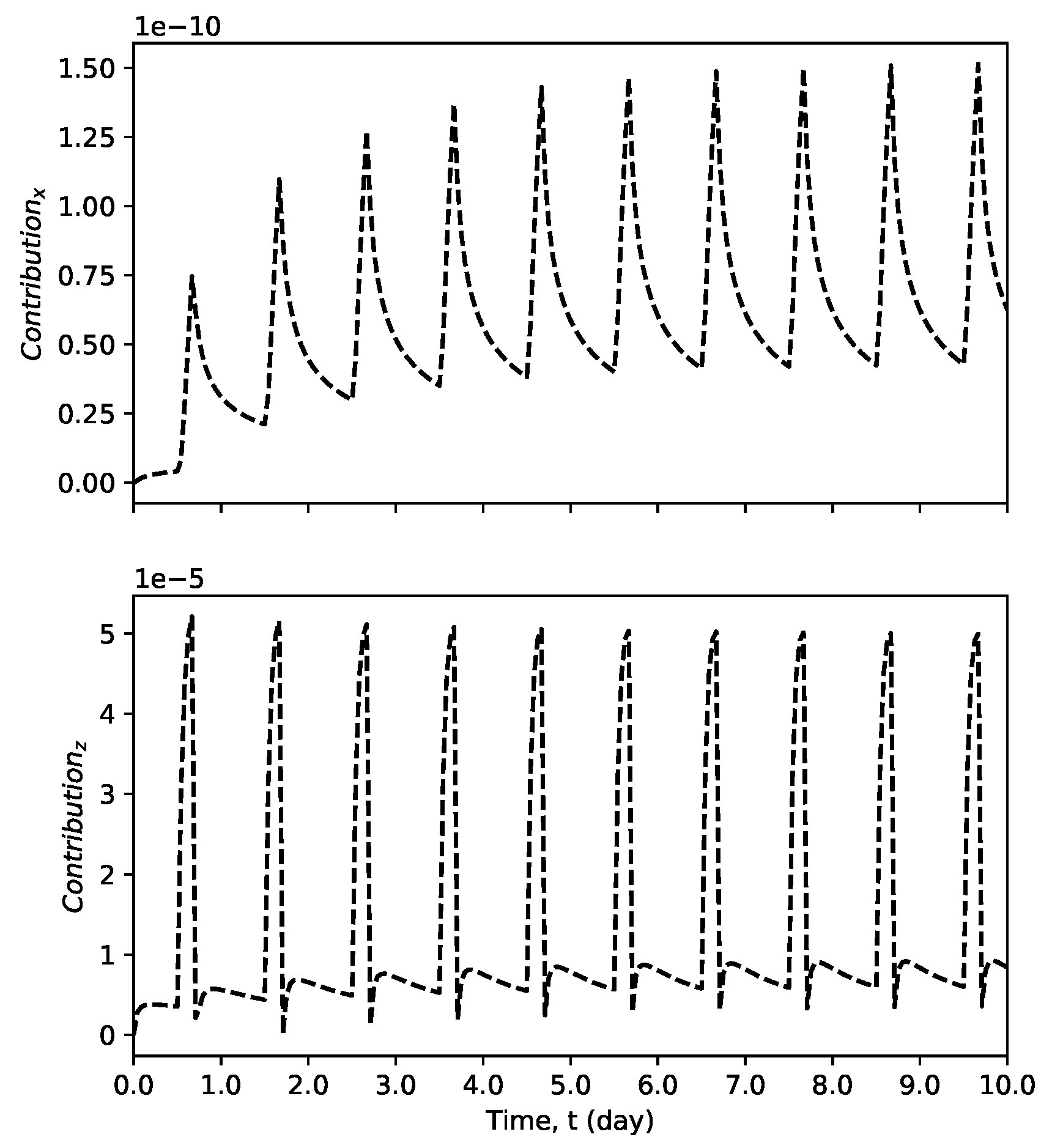
First, a quantitative result is shown to support the analysis in Section 3.3 and further motivate the decentralized framework. The trajectories of the magnitudes of terms (16) and (18) are generated under Scenario 1. The 2nd top state in the left subsystem of Model 2 is considered as $x_{i,j,k}$. The top plot of Figure A4 in Appendix A shows the trajectory of the magnitude of the term (16) and the bottom plot shows the trajectory of the magnitude of term (18). They show that the magnitude of term (18) is around $0.5\times {10}^6$ greater than the magnitude of term (16). Therefore, the horizontal interaction between the states are notably smaller, comparing to the vertical interaction between the states. This further justifies the use of DeMHE.

Next, we apply DeMHE to estimate the states and parameters of the studied field with two subsystems. The performance of DeMHE is studied under the three scenarios mentioned in Section 4.3. While the minimum number of sensors is 8, we consider that we have in total 16 sensors installed to further ensure the degree of observability. Specifically, we assume that 8 tensiometers ($N_y$) are installed in each subsystem. These sensors are installed at 5.23 cm, 13.6 cm, 22.0 cm, 30.4 cm, 38.7 cm, 47.1 cm, 55.5 cm, and 63.9 cm below the surface, which measure the 2nd, 6th, 10th, 14th, 18th, 22th, 26th and 30th states along the z direction, respectively. Eight parameters ($K_s$, ${\theta }_s$, $\alpha$, and n for both loam and sandy clay loam) of the system are to be estimated. The actual parameter values used to describe the system are shown in Table 1 and they are assumed to be constant within the investigated temporal domain. Process noise and measurement noise $({\omega }_x$ and $\nu )$ are considered in the simulations and they have zero mean and standard deviations $3\times {10}^{-6}$ m and $8\times {10}^{-3}$ m, respectively. In the design of DeMHE, MHE 1 and MHE 2 are designed for Subsystem 1 and Subsystem 2, respectively. The algorithm of MHE 1 and MHE 2 are introduced in Section 3. The initial guesses of the parameters and initial states in the estimator are listed in

Table 4. True values of initial states and parameters of the process and the initial guesses used in estimators.

	Variables	True Value	Initial Guess
MHE 1	$K_s$ (m/s)	$2.89\times {10}^{-6}$	$3.18\times {10}^{-6}$
	${\theta }_s$ (m${}^3$/m${}^3$)	0.430	0.387
	$\alpha$ (1/m)	3.60	3.24
	n	1.56	1.72
	${\theta }_r$ (m${}^3$/m${}^3$)	0.0780	0.0780
MHE 2	$K_s$ (m/s)	$3.64\times {10}^{-6}$	$4.00\times {10}^{-6}$
	${\theta }_s$ (m${}^3$/m${}^3$)	0.390	0.351
	$\alpha$ (1/m)	5.90	5.31
	n	1.48	1.62
	${\theta }_r$ (m${}^3$/m${}^3$)	0.100	0.100
MHE 1 & 2	$x_0$ (m)	−0.514	−0.617

and compared with those used in the actual system.

The estimation window sizes of both MHEs are 8 h. The weighting matrices $P^n$, $Q^n$, and $R^n$ of both MHEs are the same. Specifically, the matrices $Q^n$ and $R^n$ are designed as the covariance matrices of ${\omega }_x^n$ and ${\nu }^n$ with the standard deviations reported in Section 4.1. The diagonal elements of $Q^n$ corresponding to augmented parameters are 0, because the parameters are assumed to be temporally constant. In simulations, ${10}^{-20}$ is used to approximate the value 0 and to ensure the positive definiteness of $Q^n$. The diagonal elements of $P^n$ corresponding to the states are designed as ${(3\times {10}^{-3})}^2$ and those of parameters are configured as ${(3\times {10}^{-2})}^2$. Then by retaining the same ratio with respect to the matrices described before, $P^n$, $Q^n$, and $R^n$ are increased with a much bigger magnitude to ensure the numerical stability of the associated optimization problem. The $P^n$ matrix is constant for all the optimizations. One thing worth mentioning is that even the designed weighting matrices for the two MHEs are the same, the weighting matrices could be designed differently for different types of soil, especially when the parameter heterogeneity is significant. The constraints of the states, parameters and the model uncertainty used in the two MHEs are listed in

Table 5. Lower and upper bounds used in DeMHE.

	Variables	Lower Bounds	Upper Bounds
MHE 1	${\hat{K}}_s$$(\mathrm{m}/\mathrm{s})$	$2.31\times {10}^{-6}$	$3.47\times {10}^{-6}$
	${\hat{\theta }}_s$$({\mathrm{m}}^3/{\mathrm{m}}^3)$	0.344	0.516
	$\hat{\alpha }$$(1/\mathrm{m})$	2.88	4.32
	$\hat{n}$	1.25	1.87
MHE 2	${\hat{K}}_s$$(\mathrm{m}/\mathrm{s})$	$2.91\times {10}^{-6}$	$4.37\times {10}^{-6}$
	${\hat{\theta }}_s$$({\mathrm{m}}^3/{\mathrm{m}}^3)$	0.312	0.468
	$\hat{\alpha }$$(1/\mathrm{m})$	4.72	7.08
	$\hat{n}$	1.18	1.78
MHE 1 & 2	$\hat{x}$$\left(\mathrm{m}\right)$	−1.00	$-1.00\times {10}^{-4}$
	${\hat{\omega }}_x$	−∞	∞
	${\hat{\omega }}_p$	0.00	0.00

. The upper and lower bounds of the term ${\hat{\omega }}_p$ are 0 because the parameters are constant.

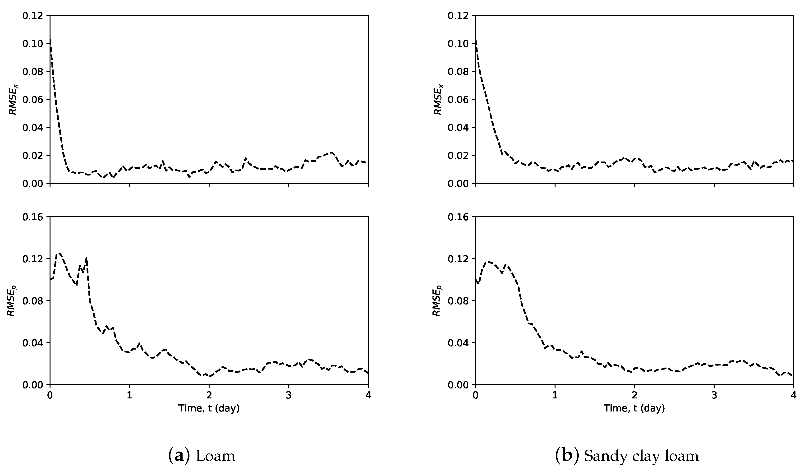
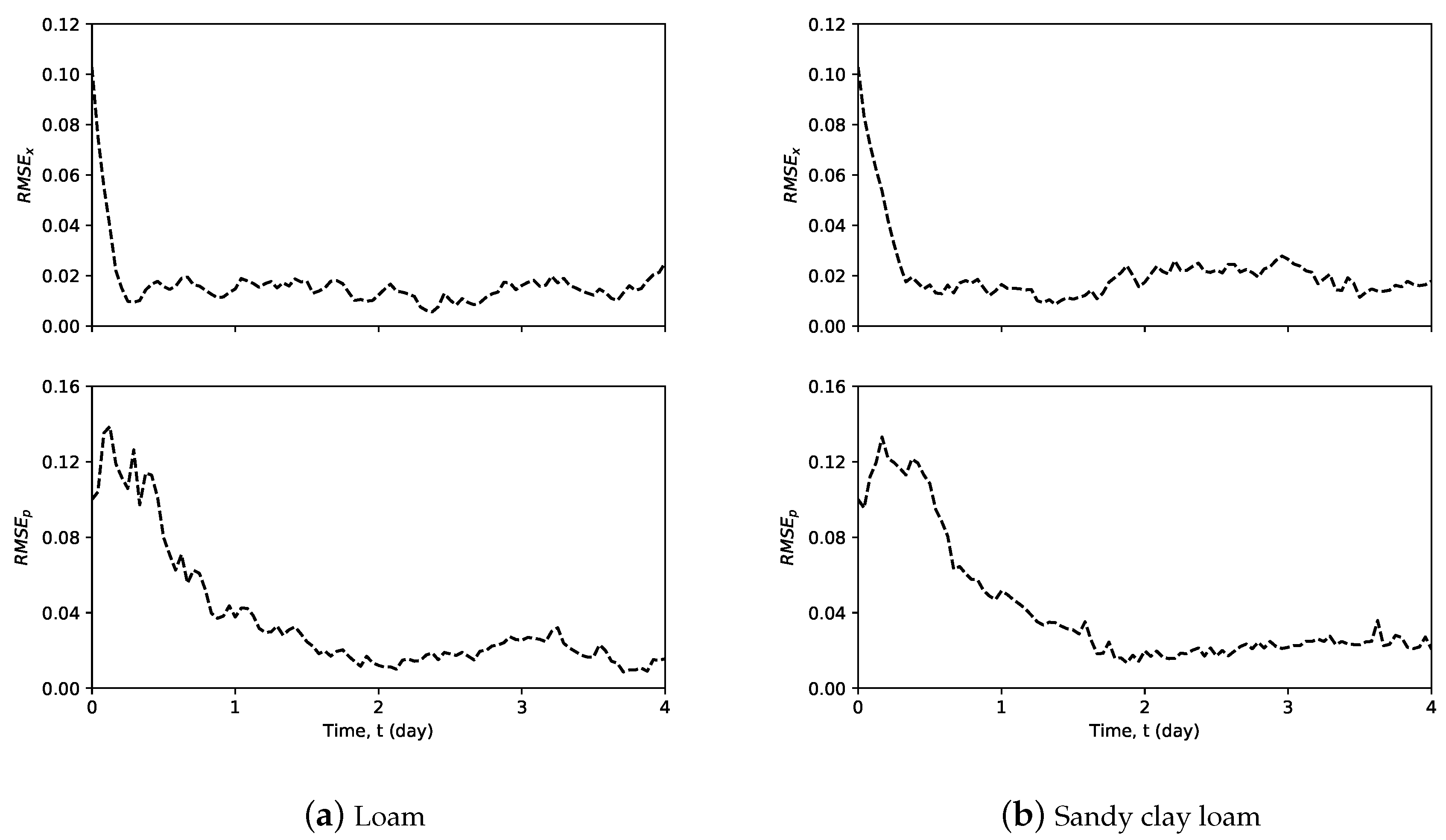
The root mean square errors [34], $RMS{E}_x$ and $RMS{E}_p$, are used to evaluate the performance of DeMHE on state and parameter estimation, respectively. They are defined as follows:

$$RMS{E}_x\left(k\right)=\sqrt{\frac{{\sum }_{i=1}^{N_x}{({\hat{x}}_i\left(k\right)-x_i\left(k\right))}^2}{N_x}}$$

(25)

$$RMS{E}_p\left(k\right)=\sqrt{\frac{{\sum }_{i=1}^{N_p}{({\hat{p}}_i\left(k\right)-p_i\left(k\right))}^2}{N_p}}.$$

(26)

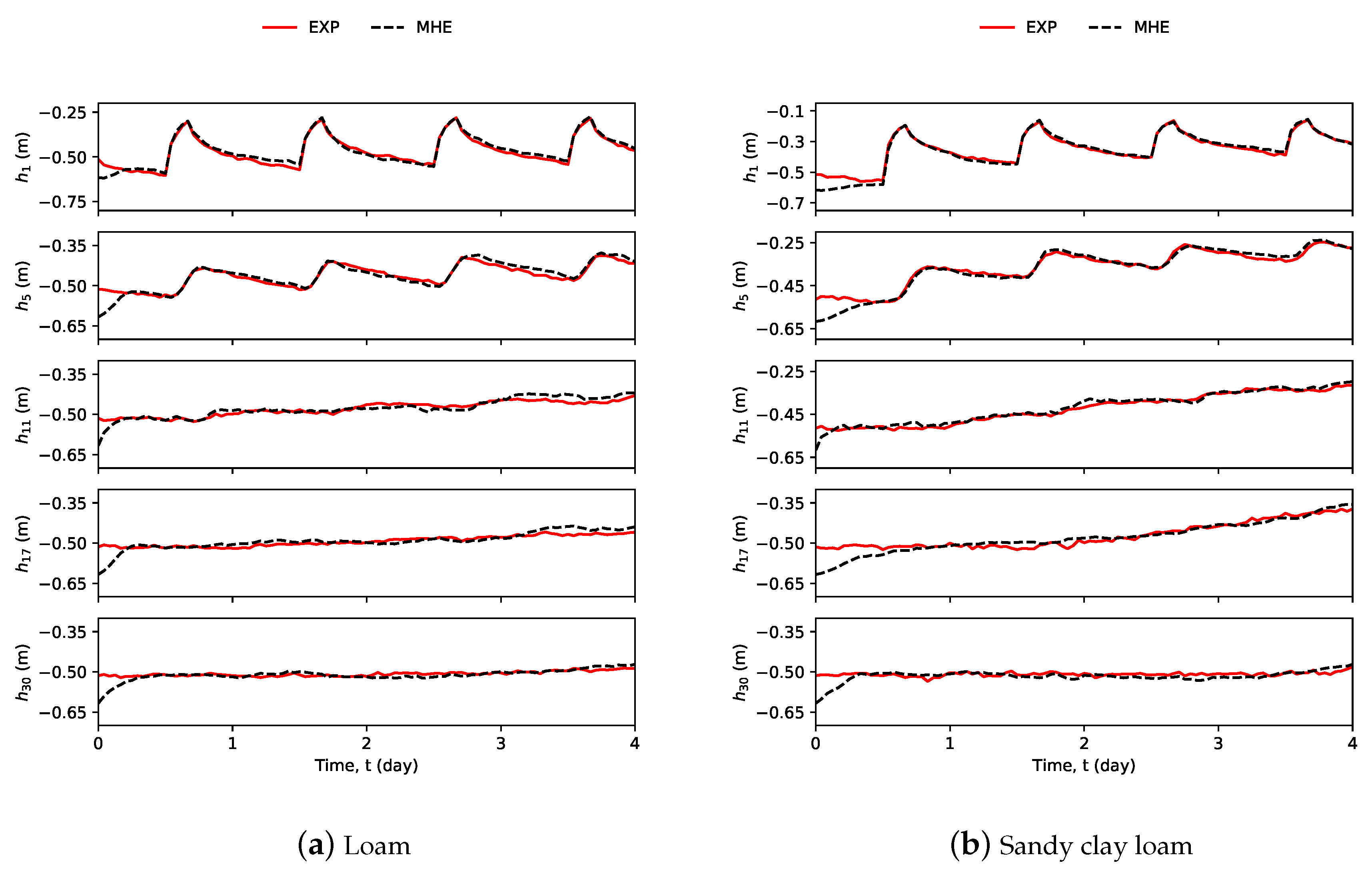
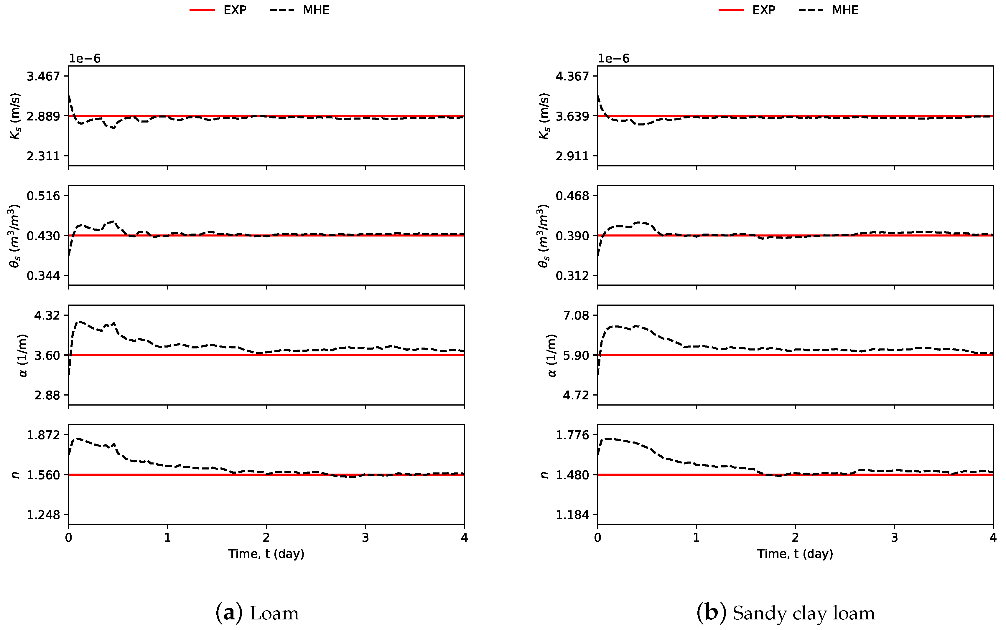
Figure 5 shows some representative estimated states and Figure 6 shows all estimated parameters using DeMHE in Scenario 1. The estimated values are also compared with their true values, which are obtained using Model 1 with both ${\Delta }x$ and ${\Delta }y$ equaling to 4 cm. In each figure, the subplot on the left side is for loam and the one on the right side is for sandy clay loam. Figure 5 shows the state trajectories of the top node and a few middle nodes and one bottom node. From the figure, it can be seen that the top node has more dynamics because it takes time for irrigated water to pass from the upper layers and to the lower layers. In terms of state estimation performance, it can be seen that DeMHE gives very good state estimates. Note that from Figure 5, it can also be seen that the estimates of the 11th state $\left(h_{11}\right)$ converge faster than the other estimates. This is because it is a sensor node. In terms of parameter estimation, Figure 6 shows the results. From the figure, it can be seen that DeMHE is capable of estimating the parameters. The trajectories of the performance indices $RMS{E}_x$ and $RMS{E}_p$ associated with the DeMHE are shown in Figure 7 and the indices for both types of soil decrease to values less than 0.02.

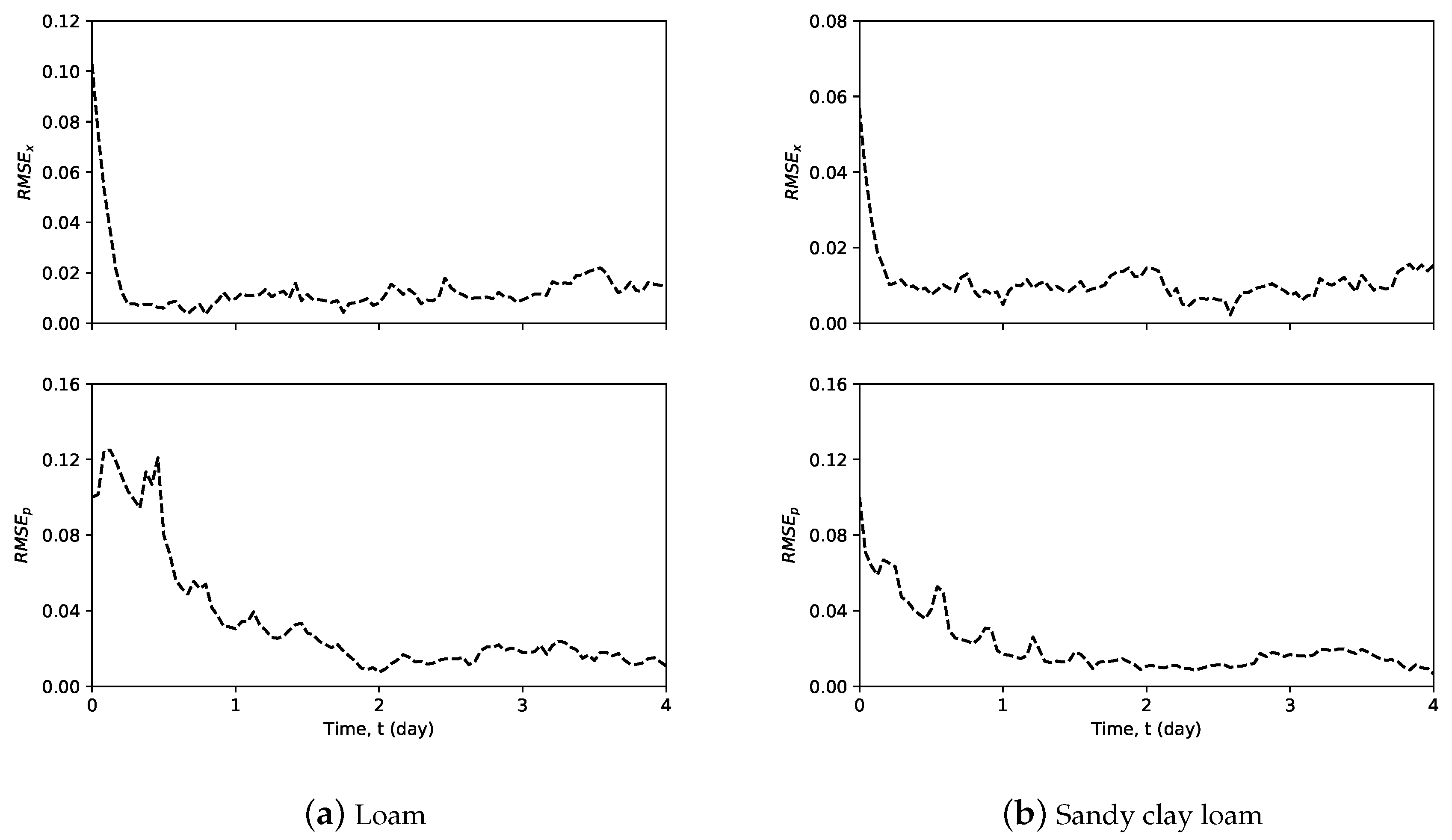
The performance of the DeMHE is also assessed under Scenarios 2 and 3. The trajectories of the performance indices $RMS{E}_x$ and $RMS{E}_p$ associated with the DeMHE under Scenario 2 and Scenario 3 are shown in Figure 8 and Figure 9, respectively. From these figures, it can be seen that the DeMHE continues to show good performance in both state and parameter estimation as in Scenario 1. The different initial conditions of the actual field in Scenario 2 or different irrigation patterns do not affect the performance of the DeMHE.

5. Conclusions

In this work, a distributed state and parameter estimation scheme developed in the framework of MHE was proposed for 3D infiltration processes with more than one types of soil. The soil parameters were assumed to be spatially heterogeneous and temporally homogeneous. Parameters were augmented as extra states for simultaneously state and parameter estimation. The appropriate parameter set which contains significant and identifiable parameters was determined based on the observability of the augmented system and the sensitivity of the outputs to the parameters. It was found that the augmented system was unobservable when a pair of saturated soil moisture and residual soil moisture of the same type of soil was presented in the system. With the sensitivity analysis showing the residual soil moisture was less important than the saturated soil moisture which is from the same soil, residual soil moistures of all presented soils were not considered in parameter estimation. For estimation, the system was decomposed into subsystems based on the soil types presented in the system. Each subsystem contained only one type of soil, hence, only four parameters (hydraulic conductivity, saturated soil moisture, and van Genuchten-Mualem parameters) of the same type of soil were presented in each subsystem. The performance of the proposed DeMHE was evaluated under the different scenarios. The simulated results showed that DeMHE was able to estimate the parameters and states very well under these scenarios. In the future, parameter and state estimation problem could be expanded and studied on an agro-hydrological system which consists of Richards’ equation, crop and atmospheric models, etc.

References

- Food and Agriculture Organization of The United Nations (FAO). AQUASTAT Main Database. Available online: http://www.fao.org/nr/water/aquastat/data/query/index.html?lang=en (accessed on 31 October 2019).
- Fischer, G.; Tubiello, F.N.; van Velthuizen, H.; Wiberg, D.A. Climate change impacts on irrigation water requirements: Effects of mitigation, 1990–2080. Technol. Forecast. Soc. Chang. 2007, 74, 1083–1107. [Google Scholar] [CrossRef] [Green Version]
- Montzka, C.; Moradkhani, H.; Weihermüller, L.; Franssen, H.J.H.; Canty, M.; Vereecken, H. Hydraulic parameter estimation by remotely-sensed top soil moisture observations with the particle filter. J. Hydrol. 2011, 399, 410–421. [Google Scholar] [CrossRef]
- Lü, H.; Yu, Z.; Zhu, Y.; Drake, S.; Hao, Z.; Sudicky, E.A. Dual state-parameter estimation of root zone soil moisture by optimal parameter estimation and extended Kalman filter data assimilation. Adv. Water Resour. 2011, 34, 395–406. [Google Scholar] [CrossRef]
- Medina, H.; Romano, N.; Chirico, G.B. Kalman filters for assimilating near-surface observations into the Richards equation–Part 2: A dual filter approach for simultaneous retrieval of states and parameters. Hydrol. Earth Syst. Sci. 2014, 18, 2521–2541. [Google Scholar] [CrossRef] [Green Version]
- Moradkhani, H.; Sorooshian, S.; Gupta, H.V.; Houser, P.R. Dual state–parameter estimation of hydrological models using ensemble Kalman filter. Adv. Water Resour. 2005, 28, 135–147. [Google Scholar] [CrossRef] [Green Version]
- Chen, W.; Huang, C.; Shen, H.; Li, X. Comparison of ensemble-based state and parameter estimation methods for soil moisture data assimilation. Adv. Water Resour. 2015, 86, 425–438. [Google Scholar] [CrossRef]
- Chaudhuri, A.; Franssen, H.J.H.; Sekhar, M. Iterative filter based estimation of fully 3D heterogeneous fields of permeability and Mualem-van Genuchten parameters. Adv. Water Resour. 2018, 122, 340–354. [Google Scholar] [CrossRef]
- Li, C.; Ren, L. Estimation of unsaturated soil hydraulic parameters using the ensemble Kalman filter. Vadose Zone J. 2011, 10, 1205–1227. [Google Scholar] [CrossRef]
- Bo, S.; Sahoo, S.R.; Yin, X.; Liu, J.; Shah, S.L. Parameter and State Estimation of One-Dimensional Infiltration Processes: A Simultaneous Approach. Mathematics 2020, 8, 134. [Google Scholar] [CrossRef] [Green Version]
- Rao, C.V.; Rawlings, J.B.; Mayne, D.Q. Constrained state estimation for nonlinear discrete-time systems: Stability and moving horizon approximations. IEEE Trans. Autom. Control 2003, 48, 246–258. [Google Scholar] [CrossRef] [Green Version]
- Yin, X.; Liu, J. Distributed moving horizon state estimation of two-time-scale nonlinear systems. Automatica 2017, 79, 152–161. [Google Scholar] [CrossRef]
- Christofides, P.D.; Scattolini, R.; de la Pena, D.M.; Liu, J. Distributed model predictive control: A tutorial review and future research directions. Comput. Chem. Eng. 2013, 51, 21–41. [Google Scholar] [CrossRef]
- Scattolini, R. Architectures for distributed and hierarchical model predictive control—A review. J. Process. Control 2009, 19, 723–731. [Google Scholar] [CrossRef]
- Daoutidis, P.; Zachar, M.; Jogwar, S.S. Sustainability and process control: A survey and perspective. J. Process. Control 2016, 44, 184–206. [Google Scholar] [CrossRef]
- Yin, X.; Liu, J. Subsystem decomposition of process networks for simultaneous distributed state estimation and control. AIChE J. 2019, 65, 904–914. [Google Scholar] [CrossRef]
- Stewart, B.T.; Venkat, A.N.; Rawlings, J.B.; Wright, S.J.; Pannocchia, G. Cooperative distributed model predictive control. Syst. Control Lett. 2010, 59, 460–469. [Google Scholar] [CrossRef]
- Venkat, A.N.; Rawlings, J.B.; Wright, S.J. Stability and optimality of distributed model predictive control. In Proceedings of the 44th IEEE Conference on Decision and Control, Seville, Spain, 12–15 December 2005; pp. 6680–6685. [Google Scholar]
- Heidarinejad, M.; Liu, J.; de la Peña, D.M.; Davis, J.F.; Christofides, P.D. Multirate Lyapunov-based distributed model predictive control of nonlinear uncertain systems. J. Process. Control 2011, 21, 1231–1242. [Google Scholar] [CrossRef]
- Dunbar, W.B. Distributed receding horizon control of dynamically coupled nonlinear systems. IEEE Trans. Autom. Control 2007, 52, 1249–1263. [Google Scholar] [CrossRef] [Green Version]
- Halvgaard, R.; Vandenberghe, L.; Poulsen, N.K.; Madsen, H.; Jørgensen, J.B. Distributed model predictive control for smart energy systems. IEEE Trans. Smart Grid 2016, 7, 1675–1682. [Google Scholar] [CrossRef]
- Zhang, J.; Liu, J. Distributed moving horizon state estimation for nonlinear systems with bounded uncertainties. J. Process. Control 2013, 23, 1281–1295. [Google Scholar] [CrossRef]
- Vadigepalli, R.; Doyle, F.J. A distributed state estimation and control algorithm for plantwide processes. IEEE Trans. Control Syst. Technol. 2003, 11, 119–127. [Google Scholar] [CrossRef]
- Yin, X.; Zeng, J.; Liu, J. Forming Distributed State Estimation Network From Decentralized Estimators. IEEE Trans. Control Syst. Technol. 2019, 27, 2430–2443. [Google Scholar] [CrossRef]
- Xie, L.; Choi, D.H.; Kar, S.; Poor, H.V. Fully distributed state estimation for wide-area monitoring systems. IEEE Trans. Smart Grid 2012, 3, 1154–1169. [Google Scholar] [CrossRef]
- Farina, M.; Ferrari-Trecate, G.; Scattolini, R. Distributed moving horizon estimation for nonlinear constrained systems. Int. J. Robust Nonlinear Control 2012, 22, 123–143. [Google Scholar] [CrossRef] [Green Version]
- Haber, A.; Verhaegen, M. Moving Horizon Estimation for Large-Scale Interconnected Systems. IEEE Trans. Autom. Control 2013, 58, 2834–2847. [Google Scholar] [CrossRef]
- Yin, X.; Decardi-Nelson, B.; Liu, J. Subsystem decomposition and distributed moving horizon estimation of wastewater treatment plants. Chem. Eng. Res. Des. 2018, 134, 405–419. [Google Scholar] [CrossRef]
- Schneider, R.; Marquardt, W. Convergence and Stability of a Constrained Partition-Based Moving Horizon Estimator. IEEE Trans. Autom. Control 2016, 61, 1316–1321. [Google Scholar] [CrossRef]
- Farina, M.; Ferrari-Trecate, G.; Scattolini, R. Distributed moving horizon estimation for sensor networks. IFAC Proc. Vol. 2009, 42, 126–131. [Google Scholar] [CrossRef]
- Van Genuchten, M.T. A closed-form equation for predicting the hydraulic conductivity of unsaturated soils. Soil Sci. Soc. Am. J. 1980, 44, 892–898. [Google Scholar] [CrossRef] [Green Version]
- Yuan, Z.; Zhao, C.; Di, Z.; Wang, W.X.; Lai, Y.C. Exact controllability of complex networks. Nat. Commun. 2013, 4, 1–9. [Google Scholar] [CrossRef] [Green Version]
- Carsel, R.F.; Parrish, R.S. Developing joint probability distributions of soil water retention characteristics. Water Resour. Res. 1988, 24, 755–769. [Google Scholar] [CrossRef] [Green Version]
- Chai, T.; Draxler, R.R. Root mean square error (RMSE) or mean absolute error (MAE)?—Arguments against avoiding RMSE in the literature. Geosci. Model Dev. 2014, 7, 1247–1250. [Google Scholar] [CrossRef] [Green Version]
Figure 1.
A schematic diagram of a 3D agro-hydrological system.
Figure 2.
A diagram illustrating spatial relation between center state and neighboring states.
Figure 3.
A schematic diagram of the proposed decentralized estimation scheme.
Figure 4.
A schematic diagram of the investigated field.
Figure 5.
Selected trajectories of the process states and estimated states using DeMHE.
Figure 6.
Trajectories of estimated parameters using DeMHE, compared with their actual values.
Figure 7.
Trajectories of RMSE measuring the estimation performance of DeMHE (Scenario 1).
Figure 8.
Trajectories of RMSE measuring the estimation performance of DeMHE for studying impact of initial conditions (Scenario 2).
Figure 9.
Trajectories of RMSE measuring the estimation performance of DeMHE for studying impact of inputs (Scenario 3).