An Extension of the Concept of Derivative: Its Application to Intertemporal Choice

Abstract

The framework of this paper is the concept of derivative from the point of view of abstract algebra and differential calculus. The objective of this paper is to introduce a novel concept of derivative which arises in certain economic problems, specifically in intertemporal choice when trying to characterize moderately and strongly decreasing impatience. To do this, we have employed the usual tools and magnitudes of financial mathematics with an algebraic nomenclature. The main contribution of this paper is twofold. On the one hand, we have proposed a novel framework and a different approach to the concept of relative derivation which satisfies the so-called generalized Leibniz’s rule. On the other hand, in spite of the fact that this peculiar approach can be applied to other disciplines, we have presented the mathematical characterization of the two main types of decreasing impatience in the ambit of behavioral finance, based on a previous characterization involving the proportional increasing of the variable “time”. Finally, this paper points out other patterns of variation which could be applied in economics and other scientific disciplines.

1. Introduction and Preliminaries

In most social and experimental sciences, such as economics, psychology, sociology, biology, chemistry, physics, epidemiology, etc., researchers are interested in finding, ceteris paribus, the relationship between the explained variable and one or more explaining variables. This relationship has not to be linear, that is to say, linear increments in the value of an independent variable does not necessarily lead to linear variations of the dependent variable. This is logical by taking into account the non-linearity of most physical or chemical laws. These circumstances motivate the necessity of introducing a new concept of derivative which, of course, generalizes the concepts of classical and directional derivatives. Consequently, the frequent search for new patterns of variations in the aforementioned disciplines justifies a new framework and a different approach to the concept of derivative, able to help in modelling the decision-making process. Let us start with some general concepts.

Let A be an arbitrary K-algebra (non necessarily commutative or associative), where K is a field. A derivation over A is a K-linear map $D:A\to A$ satisfying Leibniz’s identity:

$$D\left(ab\right)=D\left(a\right)b+aD\left(b\right).$$

It can be easily demonstrated that the sum, difference, scalar product and composition of derivations are derivations. In general, the product is not a derivation, but the so-called commutator, defined as $[D_1,D_2]=D_1{D}_2-D_2{D}_1$, is a derivation. We are going to denote by ${\mathrm{Der}}_K\left(A\right)$ the set of all derivations on A. This set has the structure of a K-module and, with the commutator operation, becomes a Lie Algebra. This algebraic notion includes the classical partial derivations of real functions of several variables and the Lie derivative with respect to a vector field in differential geometry. Derivations and differentials are important tools in algebraic geometry and commutative algebra (see [1,2,3]).

The notion of derivation was extended to the so-called $(\sigma ,\tau )$-derivation [4] for an associative $\mathbb{C}$-algebra A, where $\sigma$ and $\tau$ are two different algebra endomorphisms of A ($\sigma ,\tau \in {\mathrm{End}}_{\mathrm{Alg}}\left(A\right)$), as a $\mathbb{C}$-linear map $D:A\to A$ satisfying:

$$D\left(ab\right)=D\left(a\right)\tau \left(b\right)+\sigma \left(a\right)D\left(b\right).$$

If $\tau ={\mathrm{id}}_A$, we obtain $D\left(ab\right)=D\left(a\right)b+\sigma \left(a\right)D\left(b\right)$. In this case, we will say that D is a $\sigma$-derivation. There are many interesting examples of these generalized derivations. The q-derivation, as a q-differential operator, was introduced by Jackson [5]. In effect, let A be a $\mathbb{C}$-algebra (which could be $\mathbb{C}[z,z^{-1}]$ or various functions spaces). The two important generalizations of derivation are $D_q$ and $M_q:A\to A$, defined as:

$$\left(D_q\left(f\right)\right)\left(z\right)=\frac{f\left(qz\right)-f\left(z\right)}{qz-z}=\frac{f\left(qz\right)-f\left(z\right)}{(q-1)z}$$

and

$$M_q\left(f\right)\left(z\right)=\frac{f\left(qz\right)-f\left(z\right)}{q-1}.$$

These operations satisfy the q-deformed Leibniz’s rule, $D\left(fg\right)=D\left(f\right)g+{\sigma }_q\left(f\right)g$, where ${\sigma }_q\left(f\right)\left(z\right)=f\left(qz\right)$, i.e., the q-derivation is a $\sigma$-derivation. Observe that this formula is not symmetric as the usual one.

Now, we can compare this q-derivation with the classical h-derivation, defined by:

$$\left(D_h\left(f\right)\right)\left(z\right)=\frac{f(z+h)-f\left(z\right)}{h}.$$

In effect,

$$\underset{q\to 1}{lim}{D}_q\left(f\left(z\right)\right)=\underset{h\to 0}{lim}{D}_h\left(f\left(z\right)\right)=\frac{\mathrm{d}f\left(x\right)}{\mathrm{d}x},$$

provided that f is differentiable.

The q-derivation is the key notion of the quantum calculus which allows us to study those functions which are not differentiable. This theory has been developed by many authors and has found several applications in quantum groups, orthogonal polynomials, basic hypergeometric functions, combinatorics, calculus of variations and arithmetics [6,7].

In general, the q-derivation is more difficult to be computed. For instance, there is not a chain formula for this kind of derivation. We refer the interested reader to the books by Kac and Cheung [8], Ernst [9], and Annaby and Mansour [10] for more information about the q-derivations and q-integrals.

The q-derivation has been generalized in many directions within the existing literature. Recently, the $\beta$-derivative was introduced by Auch in his thesis [11], where $\beta \left(z\right)=az+b$, with $a\ge 1$, $b\ge 0$ and $a+b>1$, the general case being considered in [12] and continued by several scholars [13]:

$$D_{\beta }\left(f\right)\left(z\right)=\frac{f\left(\beta \right(z\left)\right)-f\left(z\right)}{\beta \left(z\right)-z},$$

where $\beta \ne z$ and $\beta :I\to I$ is a strictly increasing continuous function, $I\subseteq \mathbb{R}$. Thus, q-derivation is a particular case of this new concept. Moreover, the operator by Hahn [14,15], defined as:

$$D_{q,\omega }\left(f\right)\left(z\right)=\frac{f(qz+\omega )-f\left(z\right)}{(q-1)z+\omega },$$

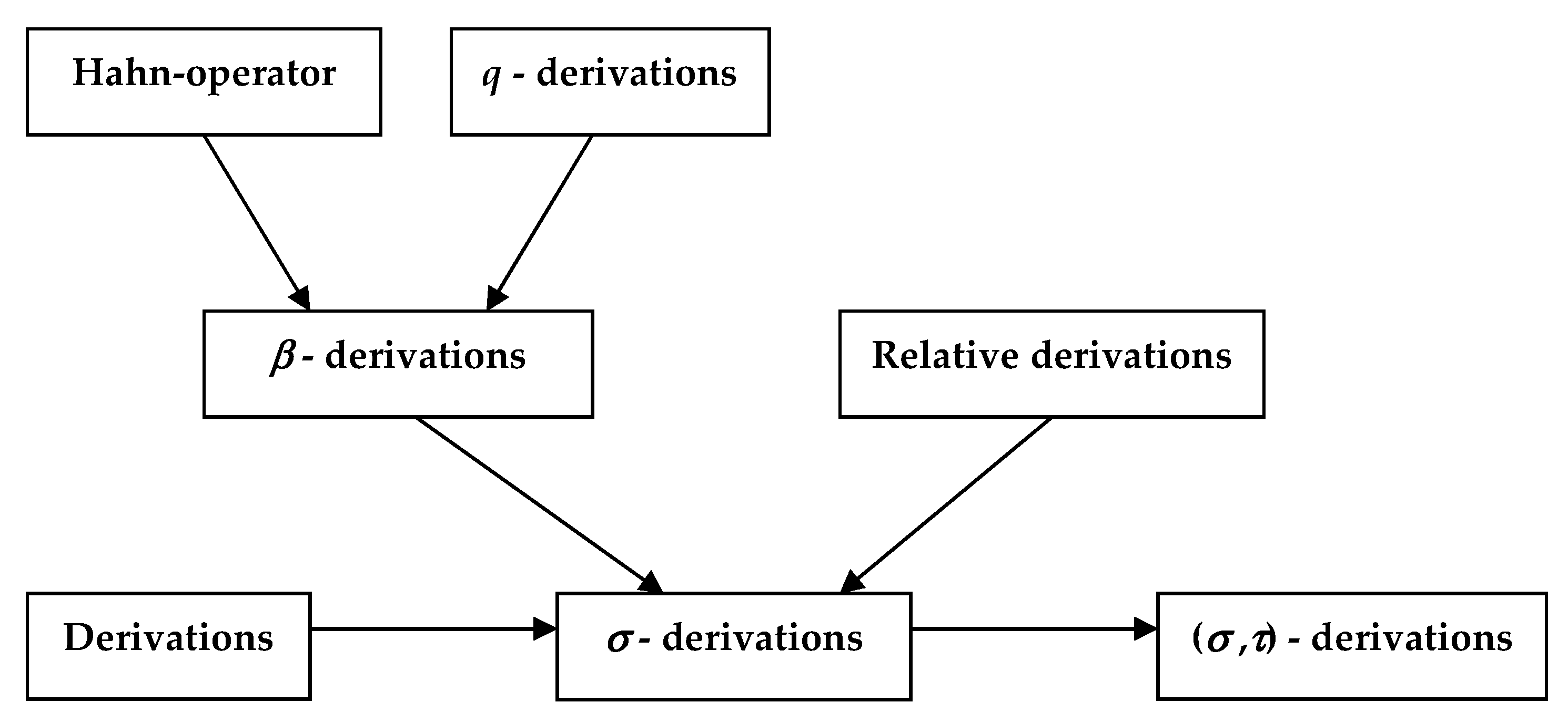
introduced to study orthogonal polynomials, is also a particular case. Another generalization of q-calculus is the so-called $(p,q)$-derivative which is a $(\sigma ,\tau )$-derivation [16].

Figure 1 summarizes the different types of derivations presented in this section and shows the relationships between them.

This paper has been organized as follows. After this Introduction, Section 2 presents the novel concept of derivation relative to a given function f. It is shown that this derivative can be embodied in the ambit of relative derivations and satisfies Leibniz’s rule. In Section 3, this new algebraic tool is used to characterize those discount functions exhibiting moderately and strongly decreasing impatience. In Section 4, the obtained results are discussed in the context of other variation patterns (quadratic, logarithmic, etc.) present in economics, finance and other scientific fields. Finally, Section 5 summarizes and concludes.

2. An Extension of the Concept of Derivative

2.1. General Concepts

Let A be a K-algebra and M be an A-module, where K is a field. Let $\sigma :A\to A$ an endomorphism of A. A $\sigma$-derivationD on M is an K-linear map

$$D:A⟶M,$$

such that

$$D\left(ab\right)=D\left(a\right)b+\sigma \left(a\right)D\left(b\right),$$

for every a and $b\in A$. From a structural point of view, let us denote by ${\mathrm{Der}}_K^{\sigma }(A,M)$ the set of all K-derivations on M. Obviously, ${\mathrm{Der}}_K^{\sigma }(A,M)$ is an A-module. In effect, if $D,D_1,D_2\in {\mathrm{Der}}_K^{\sigma }(A,M)$ and $a\in A$, then $D_1+D_2\in {\mathrm{Der}}_K^{\sigma }(A,M)$ and $aD\in {\mathrm{Der}}_K^{\sigma }(A,M)$.

In the particular case where $M=A$, D will be called a K-derivation on A, and

$${\mathrm{Der}}_K^{\sigma }(A,A):={\mathrm{Der}}_K^{\sigma }\left(A\right)$$

will be called the module of σ-derivations on A.

2.2. Relative Derivation

Let us consider the module of K-derivations on the algebra A, ${\mathrm{Der}}_K^{\sigma }\left(A\right)$. For every $D_0$ and $D\in {\mathrm{Der}}_K^{\sigma }\left(A\right)$ and $a\in A$, we can define the derivation relative to $D_0$ and a as

$$D_a(·):=D_0\left(a\right)D(·).$$

Lemma 1.

If A is commutative, then $D_a$ is a σ-derivation.

Proof. 

In effect, clearly D is K-linear and, moreover, satisfies the generalized Leibniz’s condition:

$$\begin{array}{ccc}\hfill D_a\left(xy\right)& =& D_0\left(a\right)D\left(xy\right)\hfill \\ & =& D_0\left(a\right)[D\left(x\right)y+\sigma \left(x\right)D\left(y\right)]\hfill \\ & =& D_0\left(a\right)D\left(x\right)y+\sigma \left(x\right)D_0\left(a\right)D\left(y\right)\hfill \\ & =& D_a\left(x\right)y+\sigma \left(x\right)D_a\left(y\right).\hfill \end{array}$$

This completes the proof. □

Given two $\sigma$-derivations, $D_0$ and $D\in De{r}_K^{\sigma }\left(A\right)$, we can define a map

$$\mathcal{D}:A\to De{r}_K^{\sigma }\left(A\right)$$

such that

$$\mathcal{D}\left(a\right)=D_a:=D_0\left(a\right)D.$$

Example 1.

Consider the polynomial ring $A:=K[x_1,x_2,\dots ,x_n,y_1,y_2,\dots ,y_n]$, $D_0={\partial }_{x_1}+\cdots +{\partial }_{x_n}$ and $D={\partial }_{y_1}+\cdots +{\partial }_{y_n}$. Then, for $a=x_1{y}_1+\cdots +x_n{y}_n$ and every $f\in \mathcal{D}$, one has:

$$\begin{array}{ccc}\hfill D_a\left(f\right)& =& D_0\left(a\right)D\left(f\right)\hfill \\ & =& D_0(x_1{y}_1+\cdots +x_n{y}_n)D\left(f\right)\hfill \\ & =& (y_1+\cdots +y_n)[{\partial }_{y_1}\left(f\right)+\cdots +{\partial }_{y_n}\left(f\right))].\hfill \end{array}$$

Proposition 1.

For a commutative ring A, $\mathcal{D}$ is a σ-derivation.

Proof. 

Firstly, let us see that $\mathcal{D}$ is K-linear. In effect, for every $a,b\in A$ and $k\in K$, one has:

$$\begin{array}{ccc}\hfill \mathcal{D}(a+b)& =& D_{a+b}=D_0(a+b)D\hfill \\ & =& D_0\left(a\right)D+D_0\left(b\right)D=D_a+D_b=\mathcal{D}\left(a\right)+\mathcal{D}\left(b\right)\hfill \end{array}$$

and

$$\begin{array}{ccc}\hfill \mathcal{D}\left(ka\right)& =& D_{ka}=D_0\left(ka\right)D\hfill \\ & =& k{D}_0\left(a\right)D=k{D}_a=k\mathcal{D}\left(a\right).\hfill \end{array}$$

Secondly, we are going to show that $\mathcal{D}$ satisfies the generalized Leibniz condition. In effect, for every $a,b\in A$, one has:

$$\begin{array}{ccc}\hfill \mathcal{D}\left(ab\right)& =& D_{ab}=D_0\left(ab\right)D=[D_0\left(a\right)b+\sigma \left(a\right)D_0\left(b\right)]D\hfill \\ & =& \left[D_0\left(a\right)D\right]b+\sigma \left(a\right)\left[D_0\left(b\right)D\right]=D_{a}b+\sigma \left(a\right)D_b={\mathcal{D}}_{a}b+\sigma \left(a\right)\mathcal{D}\left(b\right).\hfill \end{array}$$

Therefore, $\mathcal{D}$ is a $\sigma$-derivation. □

Now, we can compute the bracket of two relative $\sigma$-derivations $D_a$ and $D_b$, for every $a,b\in A$:

$$\begin{array}{ccc}\hfill [D_a,D_b]& =& D_a\circ D_b-D_b\circ D_a\hfill \\ & =& D_a\left[D_0\left(b\right)D\right]-D_b\left[D_0\left(a\right)D\right]\hfill \\ & =& D_0\left(a\right)D\left(D_0\left(b\right)D\right)-D_0\left(b\right)D\left(D_0\left(a\right)D\right)\hfill \\ & =& D_0\left(a\right)[D{D}_0\left(b\right)D+\sigma \left(D_0\left(b\right)\right)D^2]-D_0\left(b\right)[D{D}_0\left(a\right)D+\sigma \left(D_0\left(a\right)\right)D^2]\hfill \\ & =& [D_0\left(a\right)D{D}_0\left(b\right)-D_0\left(b\right)D{D}_0\left(a\right)]D+[D_0\left(a\right)\sigma \left(D_0\left(b\right)\right)-D_0\left(b\right)\sigma \left(D_0\left(a\right)\right])D^2.\hfill \end{array}$$

Observe that, although the bracket of two derivations is a derivation, in general it is not a relative derivation. However, if A is commutative and $\sigma$ is the identity, then the former bracket could be simplified as follows:

$$\begin{array}{ccc}[D_a,D_b]\hfill & =\hfill & [D_0\left(a\right)D{D}_0\left(b\right)-D_0\left(b\right)D{D}_0\left(a\right)]D+[D_0\left(a\right),D_0\left(b\right)]D^2\hfill \\ & =\hfill & [D_0\left(a\right)D{D}_0\left(b\right)-D_0\left(b\right)D{D}_0\left(a\right)]D.\hfill \end{array}$$

Moreover, if A is commutative and $\sigma$ is the identity, the double bracket of three derivations $D_a$, $D_b$ and $D_c$, for every $a,b,c\in A$, is:

$$\begin{array}{ccc}\hfill [[D_a,D_b],D_c]& =& [D_0\left(a\right)D{D}_0\left(b\right)-D_0\left(b\right)D{D}_0\left(a\right)]D{D}_c-D_c[D_0\left(a\right)D{D}_0\left(b\right)-D_0\left(b\right)D{D}_0\left(a\right)]D\hfill \\ & =& [D_0\left(a\right)D{D}_0\left(b\right)-D_0\left(b\right)D{D}_0\left(a\right)]D{D}_0\left(c\right)D-D_0\left(c\right)D[D_0\left(a\right)D{D}_0\left(b\right)-D_0\left(b\right)D{D}_0\left(a\right)]D\hfill \\ & =& [D_0\left(a\right)D{D}_0\left(b\right)-D_0\left(b\right)D{D}_0\left(a\right)]D{D}_0\left(c\right)D+[D_0\left(a\right)D{D}_0\left(b\right)-D_0\left(b\right)D{D}_0\left(a\right))]D_0\left(c\right)D^2\hfill \\ & =& D_0\left(c\right)\left\{D[D_0\left(a\right)D{D}_0\left(b\right)-D_0\left(b\right)D{D}_0\left(a\right)]\right\}D-D_0\left(c\right)\{D[D_0\left(a\right)D{D}_0\left(b\right)-D_0\left(b\right)D{D}_0\left(a\right)]D.\hfill \end{array}$$

Since the relative derivations are true derivations, they satisfy Jacobi’s identity, i.e., for every $a,b,c\in A$, the following identity holds:

$$[D_a,[D_b,D_c]]+[D_b,[D_c,D_a]]+[D_b,[D_a,D_b]]=0.$$

For $\sigma$ derivation one could modify the definition of the bracket as in [17] and then a Jacobi-like identity is obtained [17]. We left the details to the reader.

Given another derivation $D_1$, we can define a new relative $\sigma$-derivation $D_a^{\prime }:=D_1\left(a\right)D$. In this case, the new bracket is:

$$\begin{array}{ccc}\hfill [D_a,D_a^{\prime }]& =& D_a{D}_a^{\prime }-D_a^{\prime }{D}_a\hfill \\ & =& D_0\left(a\right)D\left(D_1\left(a\right)D\right)-D_1\left(a\right)D\left(D_0\left(a\right)D\right)\hfill \\ & =& D_0\left(a\right)[D{D}_1\left(a\right)D-\sigma \left(D_1\left(a\right)\right)D^2]-D_1\left(a\right)[D{D}_0\left(a\right)D-\sigma \left(D_0\left(a\right)\right)D^2]\hfill \\ & =& [D_0\left(a\right)D{D}_1\left(a\right)-D_1\left(a\right)D{D}_0\left(a\right)]D+[D_1\left(a\right)\sigma \left(D_0\left(a\right)\right)-D_0\left(a\right)\sigma \left(D_1\left(a\right)\right)]D^2.\hfill \end{array}$$

If A is commutative and $\sigma$ is the identity, then:

$$[D_a,D_a^{\prime }]=[D_0\left(a\right)D{D}_1\left(a\right)-D_1\left(a\right)D{D}_0\left(a\right)]D.$$

The chain rule is also satisfied for relative derivations when A is commutative. In effect, assume that, for every $f,g\in A$, the composition, $f\circ g$, is defined. Then

$$\begin{array}{ccc}\hfill D_a(f\circ g)& =& D_0(f\circ g)D(f\circ g)\hfill \\ & =& [D_0\left(f\right)\circ g]D_0\left(g\right)[D\left(f\right)\circ g]D\left(g\right)\hfill \\ & =& [D_0\left(f\right)\circ g][D\left(f\right)\circ g]D_0\left(g\right)D\left(g\right)\hfill \\ & =& [D_0\left(f\right)D\left(f\right)\circ g]D_0\left(g\right)D\left(g\right)\hfill \\ & =& [D_a\left(f\right)\circ g]D_a\left(g\right).\hfill \end{array}$$

2.3. Derivation Relative to a Function

Let $f(x,\Delta )$ be a real function of two variables x and $\Delta$ such that, for every a:

$$\underset{\Delta \to 0}{lim}f(a,\Delta )=a.$$

(1)

Let $F\left(x\right)$ be a real function differentiable at $x=a$. The derivative of F relative to f, at $x=a$, denoted by $D_f\left(F\right)\left(a\right)$, is defined as the following limit:

$$D_f\left(F\right)\left(a\right):=\underset{\Delta \to 0}{lim}\frac{F\left[f\right(a,\Delta \left)\right]-F\left(a\right)}{\Delta }.$$

(2)

In this setting, we can define $g(x,\Delta )$ as the new function, also of two variables x and $\Delta$, satisfying the following identity:

$$f(x,\Delta ):=x+g(x,\Delta ).$$

(3)

Observe that $g(x,\Delta )=f(x,\Delta )-x$ and, consequently,

$$\underset{\Delta \to 0}{lim}g(a,\Delta )=0.$$

The set of functions $g(x,\Delta )$, denoted by $\mathcal{S}$, is a subalgebra of the algebra of real-valued functions of two variables x and $\Delta$, represented by $\mathcal{A}$. In effect, it is obvious to check that, if $g,g_1,g_2\in \mathcal{S}$ and $\lambda \in \mathbb{R}$, then $g_1+g_2$, $g_1·g_2$, and $\lambda g$ belong to $\mathcal{S}$. Therefore, if $\mathcal{F}$ denotes the set of the so-defined functions $f(x,\Delta )$, we can write:

$$\mathcal{F}=\mathrm{id}+\mathcal{S},$$

(4)

where $\mathrm{id}\left(x\right)=x$ is the identity function of one variable. In $\mathcal{S}$, we can define the following binary relation:

$$g_1\sim g_2\mathrm{if},\mathrm{and}\mathrm{only}\mathrm{if},\underset{\Delta \to 0}{lim}\frac{g_1(x,\Delta )}{\Delta }=\underset{\Delta \to 0}{lim}\frac{g_2(x,\Delta )}{\Delta }.$$

(5)

Obviously, ∼ is an equivalence relation. Now, we can define $h(x,\Delta )$ as the new function also of two variables x and $\Delta$, satisfying the following identity:

$$g(x,\Delta ):=h(x,\Delta )\Delta .$$

(6)

Thus,

$$h(x,\Delta )=\frac{f(x,\Delta )-x}{\Delta }.$$

(7)

Therefore,

$$D_f\left(F\right)\left(a\right)=\underset{\Delta \to 0}{lim}\frac{F[a+h(a,\Delta )\Delta ]-F\left(a\right)}{h(a,\Delta )\Delta }\underset{\Delta \to 0}{lim}h(a,\Delta ).$$

(8)

Observe that now ${lim}_{\Delta \to 0}h(a,\Delta )$ only depends on a, whereby it can be simply denoted as $h\left(a\right)$:

$$h\left(a\right):=\underset{\Delta \to 0}{lim}h(a,\Delta ).$$

(9)

Thus, Equation (8) results in:

$$D_f\left(F\right)\left(a\right)=D\left(F\right)\left(a\right)·h\left(a\right).$$

(10)

If $f(x,\Delta )$ is derivable at $\Delta =0$, then $f(x,\Delta )$ is continuous at $\Delta =0$, whereby

$$f(a,0)=\underset{\Delta \to 0}{lim}f(a,\Delta )=a$$

(11)

and, consequently,

$$h\left(a\right)=\underset{\Delta \to 0}{lim}h(a,\Delta )=\underset{\Delta \to 0}{lim}\frac{f(a,\Delta )-f(a,0)}{\Delta }={\left.\frac{\partial f(a,\Delta )}{\partial \Delta }\right|}_{\Delta =0}.$$

(12)

Therefore,

$$D_f\left(F\right)\left(a\right)={\left.\frac{\partial f(a,\Delta )}{\partial \Delta }\right|}_{\Delta =0}D\left(F\right)\left(a\right).$$

(13)

Observe that we are representing by $D:{\mathcal{C}}^1\left(\mathbb{R}\right)\to {\mathcal{C}}^1\left(\mathbb{R}\right)$ the operator $D=\frac{\mathrm{d}}{\mathrm{d}x}$. If, additionally, the partial derivative ${\left.\frac{\partial f(a,\Delta )}{\partial \Delta }\right|}_{\Delta =0}$ is simply denoted by ${\partial }_{y=0}\left(f\right)\left(a\right)$, expression (13) remains as:

$$D_f\left(F\right)\left(a\right)={\partial }_{y=0}\left(f\right)\left(a\right)D\left(F\right)\left(a\right)={\partial }_{y=0}\left(g\right)\left(a\right)D\left(F\right)\left(a\right)$$

or, globally,

$$D_f\left(F\right)={\partial }_{y=0}\left(f\right)D\left(F\right)={\partial }_{y=0}\left(g\right)D\left(F\right).$$

Thus, $D_f:{\mathcal{C}}^1\left(\mathbb{R}\right)\to {\mathcal{C}}^1\left(\mathbb{R}\right)$ is really a derivation:

$$\begin{array}{ccc}\hfill D_f\left(FG\right)& =& {\partial }_{y=0}\left(f\right)D\left(FG\right)\hfill \\ & =& {\partial }_{y=0}\left(f\right)[D\left(F\right)G+FD\left(G\right)]\hfill \\ & =& \left[{\partial }_{y=0}\left(f\right)D\left(F\right)\right]G+F\left[{\partial }_{y=0}\left(f\right)D\left(G\right)\right]\hfill \\ & =& D_f\left(F\right)G+F{D}_f\left(G\right).\hfill \end{array}$$

Observe that $h\left(a\right)$ or ${\partial }_{y=0}\left(f\right)\left(a\right)$ represents the equivalence class including the function $g(a,\Delta )$. Moreover, the set of all suitable values of $D_f\left(F\right)\left(a\right)$ is restricted to the set

$$D\left(F\right)\left(a\right)(\mathcal{S}/\sim ),$$

where $\mathcal{S}/\sim$ is the quotient set derived from the equivalence relation ∼.

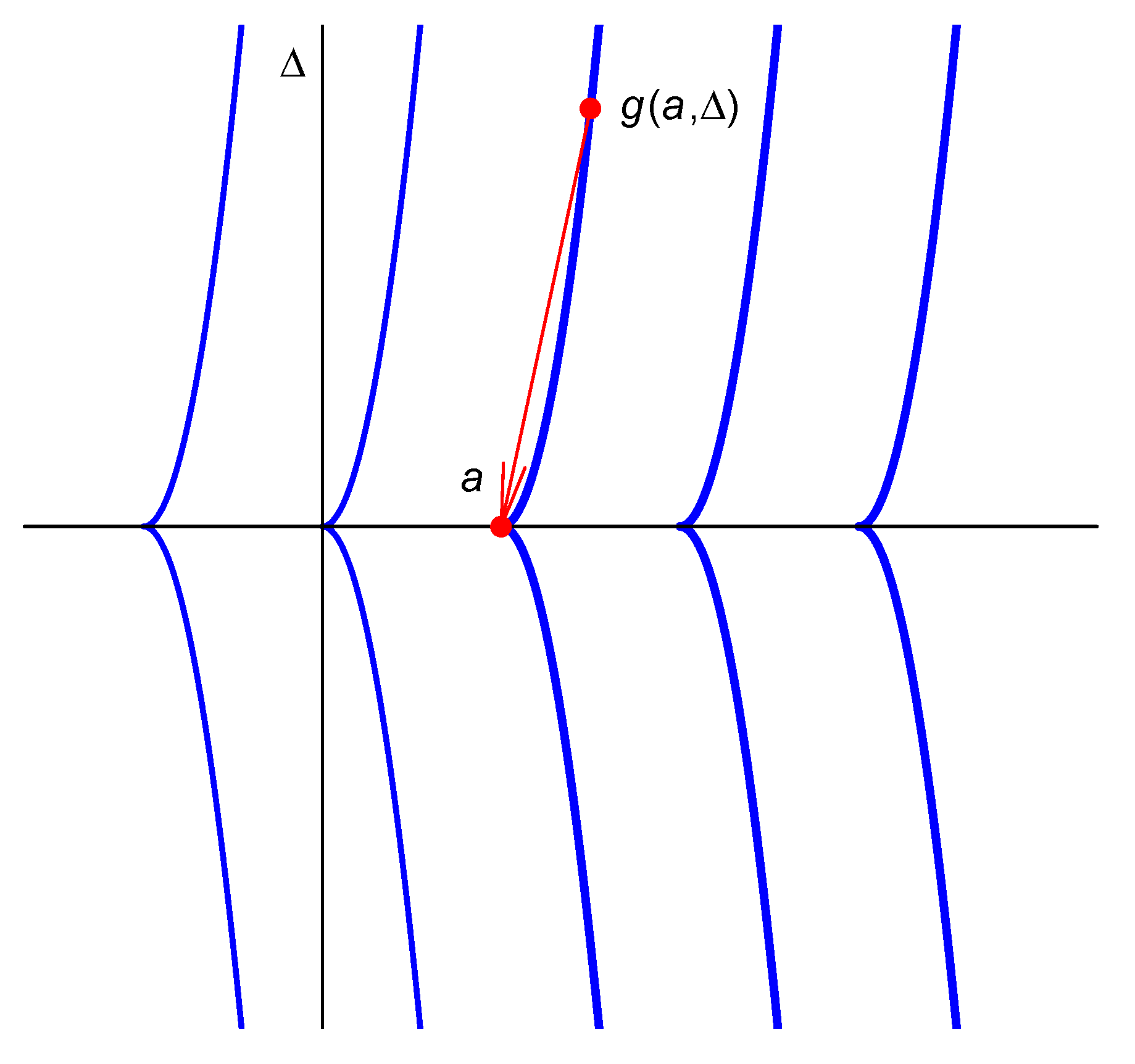
The name assigned to this derivative can be justified as follows. Observe that the graphic representation of $g(a,\Delta )$ is a surface which describes a kind of “valley” over the a-axis (that is to say, $\Delta =0$) (see Figure 2). Therefore, for every value of a, a path can be obtained by intersecting the surface with the vertical plane crossing the point $(a,0)$, giving rise to the function $g(a,\Delta )$, which represents the increment of a. As previously indicated, $g(a,\Delta )$ tend to zero as $\Delta$ approaches to zero (represented by the red arrow).

In the particular case in which

$$f(x,\Delta )=x+\Delta ,$$

(14)

obviously, one has:

$$D_f\left(F\right)\left(a\right)=D\left(F\right)\left(a\right),$$

(15)

that is to say, the derivative relative to the function $f(x,\Delta )=x+\Delta$ (absolute increments) coincides with the usual derivative.

Example 2.

Assume that (percentage increments of the variable):

$$f(x,\Delta )=x+\frac{\Delta }{x}.$$

In this case,

$$D_f\left(F\right)\left(a\right)=\frac{1}{a}D\left(F\right)\left(a\right).$$

In the context of certain scientific problems, it is interesting to characterize the variation (increase or decrease) of the so-defined derivative relative to a given function. In this case, the sign of the usual derivative of this relative derivative will be useful:

$$D\left[D_f\left(F\right)\right]=D\left[{\partial }_{y=0}\left(f\right)D\left(F\right)\right]=D\left[{\partial }_{y=0}\left(f\right)\right]D\left(F\right)+{\partial }_{y=0}\left(f\right)D^2\left(F\right).$$

(16)

Thus, if $D_f\left(F\right)$ must be increasing (resp. decreasing), then

$$D^2\left(F\right)>-\frac{D\left[{\partial }_{y=0}\left(f\right)\right]D\left(F\right)}{{\partial }_{y=0}\left(f\right)}$$

(17)

(resp. $D^2\left(F\right)<-\frac{D\left[{\partial }_{y=0}\left(f\right)\right]D\left(F\right)}{{\partial }_{y=0}\left(f\right)}$).

Example 3.

Assume that $f(x,\Delta )=ln(exp\{a\}+\Delta )$. In this case,

$$D_f\left(F\right)\left(a\right)=\frac{1}{exp\left\{a\right\}}D\left(F\right)\left(a\right).$$

The condition of increase of $D_f\left(F\right)$ leads to

$$D^2\left(F\right)>D\left(F\right).$$

3. An Application to Intertemporal Choice: Proportional Increments

This section is going to apply this new methodology to a well-known economic problem, more specifically to intertemporal choice. In effect, we are going to describe a noteworthy particular case of our derivative when the change in the variable is due to proportional instead to absolute increments. To do this, let us start with the description of the setting in which the new derivative will be applied (see [18,19]).

Let X be set ${\mathbb{R}}^{+}$ of non-negative real numbers and T a non-degenerate closed interval of $[0,+\infty )$. A dated reward is a couple $(x,t)\in X\times T$. In what follows, we will refer to x as the amount and t as the time of availability of the reward. Assume that a decision maker exhibits a continuous weak order on $X\times T$, denoted by ⪯, satisfying the following conditions (the relations ≺, ⪰, ≻ and ∼ can be defined as usual):

1.

For every $s\in T$ and $t\in T$, $(0,s)\sim (0,t)$ holds.

2.

Monotonicity: For every $t\in T$, $x\in X$ and $y\in X$, such that $x<y$, then $(x,t)\prec (y,t)$.

3.

Impatience: For every $s\in T$ and $t\in T$, such that $s<t$, and $x\in X$ then $(x,s)\succ (x,t)$.

The most famous representation theorem of preferences is due to Fishburn and Rubinstein [20]: If order, monotonicity, continuity, impatience, and separability hold, and the set of rewards X is an interval, then there are continuous real-valued functions u on X and F on the time interval T such that

$$(x,s)⪯(y,t)\mathrm{if},\mathrm{and}\mathrm{only}\mathrm{if},u\left(x\right)F\left(s\right)\le u\left(y\right)F\left(t\right).$$

Additionally, function u, called the utility, is increasing and satisfies $u\left(0\right)=0$. On the other hand, function F, called the discount function, is decreasing, positive and satisfies $F\left(0\right)=1$.

Assume that, for the decision maker, the rewards $(x,s)$ and $(y,t)$, with $s<t$, are indifferent, that is to say, $(x,s)\sim (y,t)$. Observe that, necessarily, $u\left(x\right)<u\left(y\right)$. The impatience in the interval $[s,t]$, denoted by $I(s,t)$, can be defined as the difference $u\left(y\right)-u\left(x\right)$ which is the amount that the agent is willing to loss in exchange for an earlier receipt of the reward. However, in economics the magnitudes should be defined in relative, better than absolute, terms. Thus, the impatience corresponding to the interval $[s,t]$, relatively to time and amount, should be:

$$I(s,t):=\frac{u\left(y\right)-u\left(x\right)}{(t-s)u\left(y\right)}.$$

According to [20], the following equation holds:

$$u\left(x\right)F\left(s\right)=u\left(y\right)F\left(t\right),$$

whereby

$$I(s,t)=\frac{F\left(s\right)-F\left(t\right)}{(t-s)F\left(s\right)}.$$

Observe that, in algebraic terms, $I(s,t)$ is the classical “logarithmic” derivative, with minus sign, of F at time s:

$$I(s,t)=-\left(\frac{D_{t-s}\left(F\right)}{F}\right)\left(s\right),$$

where $D_{t-s}$ is the classical h-derivation, with $h=t-s$. However, in finance, the most employed measure of impatience is given by the limit of $I(s,t)$ when t tends to s, giving rise to the well-known concept of instantaneous discount rate, denoted by $\delta \left(s\right)$:

$$\delta \left(s\right):=-\underset{t\to s}{lim}\left(\frac{D_{t-s}\left(F\right)}{F}\right)\left(s\right)=-D(lnF)\left(s\right).$$

For a detailed information about the different concepts of impatience in intertemporal choice, see [21]. The following definition introduces a central concept to analyze the evolution of impatience with the passage of time.

Definition 1

([19]). A decision-maker exhibiting preferences ⪯ has decreasing impatience (DI) if, for every $s<t$, $k>0$ and $0<x<y$, $(x,s)\sim (y,t)$ implies $(x,s+k)⪯(y,t+k)$.

A consequence is that, under the conditions of Definition 1, given $\sigma >0$, there exists $\tau =\tau \left(\sigma \right)>\sigma$ such that

$$(x,s+\sigma )\sim (y,t+\tau ).$$

The existence of $\tau$ is guaranteed when, as usual, the discount function is regular, i.e., satisfies ${lim}_{t\to \infty }F\left(t\right)=0$. A specific case of DI is given by the following definition.

Definition 2

([19]). A decision-maker exhibiting decreasing impatience has strongly decreasing impatience if $s\tau \ge t\sigma$.

The following proposition provides a nice characterization of strongly decreasing impatience.

Proposition 2

([22]). A decision-maker exhibiting preferences ⪯ has strongly decreasing impatience if, and only if, for every $s<t$, $\lambda >1$ and $0<x<y$, $(x,s)\sim (y,t)$ implies $(x,\lambda s)\prec (y,\lambda t)$.

Definition 3.

Let $F\left(t\right)$ be a discount function differentiable in its domain. The elasticity of $F\left(t\right)$ is defined as:

$${ϵ}_F\left(t\right):=t\frac{D\left(F\right)\left(t\right)}{F\left(t\right)}=tD(lnF)\left(t\right)=-t\delta \left(t\right).$$

Theorem 1.

A decision-maker exhibiting preferences ⪯ has strongly decreasing impatience if, and only if, $D^2\left(F\right)>-\frac{D\left(F\right)}{\mathrm{id}}$.

Proof. 

In effect, for every $s<t$, $\lambda >1$ and $0<x<y$, by Proposition 1, $(x,s)\sim (y,t)$ implies $(x,\lambda s)\prec (y,\lambda t)$. Consequently,

$$u\left(x\right)F\left(s\right)=u\left(y\right)F\left(t\right)$$

and

$$u\left(x\right)F\left(\lambda s\right)<u\left(y\right)F\left(\lambda t\right).$$

By dividing the left-hand sides and the right-hand sides of the former inequality and equality, one has:

$$\frac{F\left(\lambda s\right)}{F\left(s\right)}<\frac{F\left(\lambda t\right)}{F\left(t\right)},$$

from where:

$$lnF\left(\lambda s\right)-lnF\left(s\right)<lnF\left(\lambda t\right)-lnF\left(t\right).$$

As $\lambda >1$, we can write $\lambda :=1+\Delta$, with $\Delta >0$, and so:

$$lnF\left(\right(1+\Delta \left)s\right)-lnF\left(s\right)<lnF\left(\right(1+\Delta \left)t\right)-lnF\left(t\right).$$

By dividing both member of the former inequality by $\Delta$ and letting $\Delta \to 0$, one has:

$$D_f\left(F\right)\left(s\right)\le D_f\left(F\right)\left(t\right),$$

where $f(x,\Delta ):=(1+\Delta )x$. Therefore, the function $D_f\left(F\right)$ is increasing, whereby:

$$D\left[D_f\left(F\right)\right]\ge 0.$$

In order to calculate $D_f\left(F\right)$, take into account that now there is a proportional increment of the variable, that is to say:

$$f(x,\Delta )=(1+\Delta )x.$$

Thus,

$$D_f\left(F\right)\left(a\right)=aD\left(F\right)\left(a\right)$$

or, globally,

$$D_f\left(F\right)=\mathrm{id}D\left(F\right).$$

Consequently, $\mathrm{id}D\left(F\right)$ is increasing, whereby:

$$D\left[ID\left(F\right)\right]=D\left(F\right)+\mathrm{id}{D}^2\left(F\right)>0,$$

from where:

$$D^2\left(F\right)>-\frac{D\left(F\right)}{\mathrm{id}}.$$

The proof of the converse implication is obvious. □

Example 4.

The discount function $F\left(t\right)=exp\{-arctan(t\left)\right\}$ exhibits strongly decreasing impatience. In effect, simple calculation shows that:

• $D\left(F\right)\left(a\right)=-\frac{1}{1+a^2}exp\{-arctan\left(t\right)\}$.
• $D^2\left(F\right)\left(a\right)=\frac{1+2a}{1+a^2}exp\{-arctan\left(t\right)\}$.

In this case, the inequality $D^2\left(F\right)>-\frac{D\left(F\right)}{\mathrm{id}}$ results in $a^2+a-1>0$ which holds for $a>\frac{-1+\sqrt{5}}{2}$.

The following result can be derived from Theorem 1 [22].

Corollary 1.

A decision-maker exhibiting preferences ⪯ has strongly decreasing impatience if, and only if, ${ϵ}_F$ is decreasing.

Proof. 

It is immediate, taking into account that $\mathrm{id}D\left(F\right)$ is increasing. As F is decreasing, then $\mathrm{id}\frac{D\left(F\right)}{F}$ is increasing and

$$ϵ=-\mathrm{id}\delta$$

is decreasing. The proof of the converse implication is obvious. □

Another specific case of DI is given by the following definition.

Definition 4

([19]). A decision-maker exhibiting decreasing impatience has moderately decreasing impatience if $s\tau <t\sigma$.

The following corollary provides a characterization of moderately decreasing impatience.

Corollary 2

([22]). A decision-maker exhibiting preferences ⪯ has moderately decreasing impatience if, and only if, for every $s<t$, $k>0$, $\lambda >1$ and $0<x<y$, $(x,s)\sim (y,t)$ implies $(x,s+k)⪯(y,t+k)$ but $(x,\lambda s)⪰(y,\lambda t)$.

Corollary 3.

A decision-maker exhibiting preferences ⪯ has moderately decreasing impatience if, and only if, $\frac{{\left[D\left(F\right)\right]}^2}{F}<D^2\left(F\right)\le -\frac{D\left(F\right)}{id}$.

Proof. 

It is an immediate consequence of Theorem 1 and of the fact that, in this case, $\delta =-\frac{D\left(F\right)}{F}$ is decreasing. □

The following result can be derived from Corollary 3 [22].

Corollary 4.

A decision-maker exhibiting preferences ⪯ has moderately decreasing impatience f, and only if, ${ϵ}_F$ is increasing but δ is decreasing.

4. Discussion

In this paper, we have introduced a new modality of relative derivation, specifically the so-called derivation of $F\left(x\right)$ relative to a function $f(x,\Delta ):=x+g(x,\Delta )$, where $g(x,\Delta )$ represents the increments in the variable x. Obviously, this novel concept generalizes the two most important derivatives used in differential calculus:

• The classical derivative, whose increments are defined as $g(x,\Delta )=\Delta$.
• The directional derivative, characterized by linear increments: $g(x,\Delta )=k\Delta$, $k\in \mathbb{R}$.

It is easy to show that, in the former cases, Equation (13) leads to the well-known expressions of these two derivatives. In this paper, we have gone a step further and have considered proportional variations of the independent variable. These increments appear in the so-called sensitivity analysis which is a financial methodology which determines how changes of a variable can affect variations of another variable. This method, also called simulation analysis, is usually employed in financial problems under uncertainty contexts and also in econometric regressions.

In effect, in some economic contexts, percentage variations of the independent variable are analyzed. For example, the elasticity is the ratio of the percentage variations of two economic magnitudes. In linear regression, if the explanatory and the explained variables are affected by the natural logarithm, it is noteworthy to analyze the percentage variation of the dependent variable compared to percentage changes in the value of an independent variable. In this case, we would be interested in analyzing the ratio:

$$\frac{f(x+\Delta x)-f\left(x\right)}{f\left(x\right)},$$

when $\frac{\Delta x}{x}=\lambda$, for a given $\lambda$. Thus, the former ratio remains as:

$$\frac{f(x+\lambda x)-f\left(x\right)}{f\left(x\right)}.$$

In another economic context, Karpoff [23], when searching the relationship between the price and the volume of transactions of an asset in a stock market, suggests quadratic and logarithmic increments:

• Quadratic increments aim to determine the variation of the volume when quadratic changes in the price of an asset have been considered. In this case,

  $$g(x,\Delta )={(x+\Delta )}^2-x^2$$

  and so

  $${\partial }_{y=0}\left(f\right)\left(a\right)=2a.$$
• Logarithmic increments aim to find the variation of the volume when considering quadratic changes in the price of an asset. In this case,

  $$g(x,\Delta )=ln(x+\Delta )-lnx$$

  and so

  $${\partial }_{y=0}\left(f\right)\left(a\right)=\frac{1}{a}.$$

Figure 3 summarizes the different types of increments discussed in this section.

Indeed, some other variation models could be mentioned here. Take into account that some disciplines, such as biology, physics or economics, might be interested in explaining the increments in the dependent variable by using alternative patterns of variation. For example, think about a particle which is moving by following a given trajectory. In this context, researchers may be interested in knowing the behavior of the explained variable when the particle is continuously changing its position according to a given function.

5. Conclusions

This paper has introduced the novel concept of derivative of a function relative to another given function. The manuscript has been divided into two parts. The first part is devoted to the algebraic treatment of this concept and its basic properties in the framework of other relative derivatives. Moreover, this new derivative has been put in relation with the main variants of derivation in the field of abstract algebra. Given two $\sigma$-derivations over a K-algebra A, where K is a field, a relative $\sigma$-derivation has been associated to any function. This construction is, in fact, a derivation from A to the A-module of $\sigma$-derivations. Specifically, if $\sigma$ is the identity of the algebra, these derivations can be applied to the theory of intertemporal choice.

The second part deals with the mathematical characterization of the so-called “strongly” and “moderately decreasing impatience” based on previous characterizations involving the proportional increasing of the variable “time”. In effect, a specific situation, the case of proportional increments, plays a noteworthy role in economics, namely in intertemporal choice, where the analysis of decreasing impatience is a topic of fundamental relevance. In effect, the proportional increment of time is linked to the concept of strongly and moderately decreasing impatience. Therefore, the calculation of derivatives relatively to this class of increments will allow us to characterize these important modalities of decreasing impatience.

Moreover, after providing a geometric interpretation of this concept, this derivative has been calculated relatively to certain functions which represent different patterns of variability of the main variable involved in the problem.

Observe that, according to Fishburn and Rubinstein [20], the continuity of the order relation implies that functions F and u are continuous but not necessarily derivable. Indeed, this is a limitation of the approach presented in this paper which affects both function F and the variation pattern g. A further research could be to analyze the case of functions which are differentiable except at possibly a finite number of points in its domain.

Finally, apart from this financial application, another future research line is the characterization of other financial problems with specific models of variability. In this way, we can point out the proportional variability of reward amounts [24].

References

- Kunz, E. Kähler Differential; Springer: Berlin, Germany, 1986. [Google Scholar]
- Eisenbud, D. Commutative Algebra with a View toward Algebraic Geometry, 3rd. ed.; Springer: Berlin, Germany, 1999. [Google Scholar]
- Matsumura, H. Commutative Algebra; Mathematics Lecture Note Series; W. A. Benjamin: New York, NY, USA, 1970. [Google Scholar]
- Jacobson, N. Structure of Rings; Amer. Math. Soc. Coll. Pub. 37; Amer. Math. Soc: Providence, RI, USA, 1956. [Google Scholar]
- Jackson, F.H. q-difference equations. Am. J. Math 1910, 32, 305–314. [Google Scholar] [CrossRef]
- Chakrabarti, R.; Jagannathan, R.; Vasudevan, R. A new look at the q-deformed calculus. Mod. Phys. Lett. A 1993, 8, 2695–2701. [Google Scholar] [CrossRef]
- Haven, E. Itô’s lemma with quantum calculus (q-calculus): Some implications. Found. Phys. 2011, 41, 529–537. [Google Scholar] [CrossRef]
- Kac, V.; Cheung, P. Quantum Calculus; Springer: Berlin, Germany, 2002. [Google Scholar]
- Ernst, T. A Comprehensive Treatment of q-Calculus; Birkhäuser: New York, NY, USA, 2012. [Google Scholar]
- Annaby, M.; Mansour, Z.S. q-Fractional Calculus and Equations; Lecture Notes in Mathematics, 2056; Springer: New York, NY, USA, 2012. [Google Scholar]
- Auch, T. Development and Application of Difference and Fractional Calculus on Discrete Time Scales. Ph.D. Thesis, University of Nebraska-Lincoln, Lincoln, NE, USA, 2013. [Google Scholar]
- Hamza, A.; Sarhan, A.; Shehata, E.; Aldwoah, K.A. General quantum difference calculus. Adv. Differ. Equ. 2015, 2015, 1–19. [Google Scholar] [CrossRef] [Green Version]
- Faried, N.; Shehata, E.M.; El Zafarani, R.M. On homogeneous second order linear general quantum difference equations. J. Inequalities Appl. 2017, 2017, 198. [Google Scholar] [CrossRef] [PubMed]
- Hahn, W. On orthogonal polynomials satisfying a q-difference equation. Math. Nachr. 1949, 2, 4–34. [Google Scholar] [CrossRef]
- Hahn, W. Ein Beitrag zur Theorie der Orthogonalpolynome. Monatshefte Math. 1983, 95, 19–24. [Google Scholar] [CrossRef]
- Gupta, V.; Rassias, T.M.; Agrawal, P.N.; Acu, A.M. Basics of Post-Quantum Calculus. In Recent Advances in Constructive Approximation Theory. Springer Optimization and its Applications; Springer: Berlin, Germany, 2018; Volume 138. [Google Scholar]
- Hartwig, J.T.; Larsson, D.; Silvestrov, S.D. Deformations of Lie algebras using σ-derivations. J. Algebra 2006, 295, 314–361. [Google Scholar] [CrossRef] [Green Version]
- Baucells, M.; Heukamp, F.H. Probability and time trade-off. Manag. Sci. 2012, 58, 831–842. [Google Scholar] [CrossRef]
- Rohde, K.I.M. Measuring decreasing and increasing impatience. Manag. Sci. 2018, 65, 1455–1947. [Google Scholar] [CrossRef] [Green Version]
- Fishburn, P.C.; Rubinstein, A. Time preference. Int. Econ. Rev. 1982, 23, 677–694. [Google Scholar] [CrossRef]
- Cruz Rambaud, S.; Muñoz Torrecillas, M.J. Measuring impatience in intertemporal choice. PLoS ONE 2016, 11, e0149256. [Google Scholar] [CrossRef] [PubMed] [Green Version]
- Cruz Rambaud, S.; González Fernández, I. A measure of inconsistencies in intertemporal choice. PLoS ONE 2019, 14, e0224242. [Google Scholar] [CrossRef] [PubMed]
- Karpoff, J.M. The relation between price changes and trading volume: A survey. J. Financ. Quant. Anal. 1987, 22, 109–126. [Google Scholar] [CrossRef]
- Anchugina, N.; Matthew, R.; Slinko, A. Aggregating Time Preference with Decreasing Impatience; Working Paper; University of Auckland: Auckland, Australia, 2016. [Google Scholar]
Figure 1.
Chart of the different revised derivations.
Figure 2.
Plotting function .
Figure 3.
Chart of the different types of increments.
© 2020 by the authors. Licensee MDPI, Basel, Switzerland. This article is an open access article distributed under the terms and conditions of the Creative Commons Attribution (CC BY) license (http://creativecommons.org/licenses/by/4.0/).
Share and Cite
MDPI and ACS Style
Cruz Rambaud, S.; Torrecillas Jover, B. An Extension of the Concept of Derivative: Its Application to Intertemporal Choice. Mathematics 2020, 8, 696. https://0-doi-org.brum.beds.ac.uk/10.3390/math8050696
AMA Style
Cruz Rambaud S, Torrecillas Jover B. An Extension of the Concept of Derivative: Its Application to Intertemporal Choice. Mathematics. 2020; 8(5):696. https://0-doi-org.brum.beds.ac.uk/10.3390/math8050696
Chicago/Turabian StyleCruz Rambaud, Salvador, and Blas Torrecillas Jover. 2020. "An Extension of the Concept of Derivative: Its Application to Intertemporal Choice" Mathematics 8, no. 5: 696. https://0-doi-org.brum.beds.ac.uk/10.3390/math8050696
Note that from the first issue of 2016, this journal uses article numbers instead of page numbers. See further details here.