Preview Control for MIMO Discrete-Time System with Parameter Uncertainty

Abstract

We consider the problems of state feedback and static output feedback preview controller (PC) for uncertain discrete-time multiple-input multiple output (MIMO) systems based on the parameter-dependent Lyapunov function and the linear matrix inequality (LMI) technique in this paper. First, for each component of a reference signal, an augmented error system (AES) containing previewed information is constructed via the difference operator and state augmentation technique. Then, for the AES, the state feedback and static output feedback are introduced, and when considering the output feedback, a previewable reference signal is utilized by modifying the output equation. The preview controllers’ parameter matrices can be achieved from the solution of LMI problems. The superiority of the PC is illustrated via two numerical examples.

1. Introduction

In the field of control, there are many effective control methods, for example, optimal control [1], learning control [2], tracking control [3], and repetitive control [4] and so on. In many practical problems, future information is always known completely or partially, such as a vehicle driving path, scheduled flight route of an aircraft, and machining rules of a machine tool. Preview control can fully utilize the future values of these previewed signals to improve the control performance [5,6]. The preview control was first proposed by Sheridan in 1966 [7], and Bender [8] applied preview control theory to a vehicle suspension system. The field of preview control has attracted researchers and has been studied since the 1970s (see, the papers [9,10,11,12,13]). For a linear constant preview control system, LQR-based design methods have been most widely studied, e.g., [14,15,16,17,18,19,20]. However, the presence of an unknown disturbance or uncertain system model can cause degraded performance or even loss of closed-loop stability. To deal with this problem, robust preview control has received considerable attention [21,22,23,24,25,26,27]. In recent years, the integration of preview control and other control methods has attracted much attention. For example, in [28,29], the analysis and design problems of preview repetitive control for discrete system have been investigated. A fault-tolerant control theory was combined with preview control in [30,31]. In [32], the preview control concept was added to the Lipschitz non-linear system to consider the preview tracking control problems. Of course, preview control has attracted researchers for its applications in varied areas, e.g., wind turbine blade-pitch control [33], autonomous vehicle guidance [34], robotics [35], and so on.

With the rapid development of computer, electronics and information technology, industrial systems are becoming larger and more complex. Therefore, it is more interesting to consider the control problem of MIMO systems. For example, the preview control problem of MIMO systems was studied in [36] by combining linear quadratic optimal theory with the AES method. However, the dimension of an AES is high and the calculation is complex. In addition, through numerical simulations, we find that the preview control effect is not ideal when the reference signal is a vector, as in [11,13,15,36,37]. The components of the reference signal influence each other, and the influence is often negative. However, for a high-dimensional reference signal, the AES constructed in [11,13,15,36,37] not only has a high dimension, but the component signals also share the same preview length.

In this paper, robust PC design methods are proposed for MIMO discrete systems. First, the construction of an AES including previewable signals is carried out. Then, sufficient conditions of closed-loop systems and the PC design methods are proposed. The main contributions of our preview control scheme are summarized as follows: (i) The AES of a MIMO uncertain discrete-time system is successfully constructed from a new perspective. It not only constructs a lower-dimensional error system, but it also provides optional preview lengths. (ii) Our desired PC design method can avoid the negative influence of reference signal components on each other, and then effectively improve the tracking performance. (iii) Our design additionally allows the system output matrices to be non-common and have uncertainties. Finally, the simulation results clearly validate the superiority of the proposed PC.

Notation. $A>0$: symmetric and positive definite matrix $A$. $A^T$ denotes the matrix transposition of $A$. The symbol $\ast$ denotes the entries of matrices implied by symmetry. $sym(A)$ means $A+A^T$. $I$ and $0$: identity matrix and zero matrix of appropriate dimensions, respectively.

2. Problem Formulation

Consider the uncertain discrete-time system

$$\{\begin{array}{c}x(k+1)=A(\theta )x(k)+B(\theta )u(k),\\ y(k)=C(\theta )x(k)+D(\theta )u(k),\end{array}$$

(1)

where $x(k)\in R^n$, $u(k)\in R^m$ and $y(k)\in R^q$ are respectively the state vector, input control vector, and output vector.

$y(k)={\left[\begin{array}{cccc}{y}_1(k)& y_2(k)& \cdots & y_q(k)\end{array}\right]}^T$, $C^i(\theta )$, and $D^i(\theta )$ represent the $i$ $(i=1,2,\cdots ,q)$ row of matrices $C(\theta )$ and $D(\theta )$, respectively. Then, we can have

$$y_i(k)=C^i(\theta )x(k)+D^i(\theta )u(k)$$

(2)

A1: The uncertain matrices are given by

$$\left[\begin{array}{cccc}A(\theta )& B(\theta )& C(\theta )& D(\theta )\end{array}\right]={\displaystyle \sum _{j=1}^s{\theta }_j}\left[\begin{array}{cccc}{A}_j& B_j& C_j& D_j\end{array}\right]$$

(3)

where $A_j$, $B_j$, $C_j$, and $D_j$ $(j=1,2,\cdots ,s)$ are matrices with appropriate dimensions. $\theta ={\left[\begin{array}{cccc}{\theta }_1& {\theta }_2& \cdots & {\theta }_s\end{array}\right]}^T\in R^s$ is the parameter vector and satisfies

$$\theta \in \Theta :=\left\{\theta \in R^s|{\theta }_j\ge 0,(j=1,2,\cdots ,s),{\displaystyle \sum _{j=1}^s{\theta }_j}=1\right\}$$

(4)

A2: Let $r(k)={\left[\begin{array}{cccc}{r}_1(k)& r_2(k)& \cdots & r_q(k)\end{array}\right]}^T\in R^q$ be the reference signal. Assume that the component reference signal $r_i(k)$ $(i=1,2,\cdots q)$ is available from current time $k$ to $k+{\mathrm{h}}_i$. The future values are assumed not to change beyond $k+{\mathrm{h}}_i$, namely,

$$r_i(k+j)=r_i(k+{\mathrm{h}}_i),(j\ge {\mathrm{h}}_i+1)$$

where ${\mathrm{h}}_i$ is the preview length.

Remark 1.

It should be noted that A2 is an assumption about $r_i(k)$ $(i=1,2,\cdots ,q)$ rather than $r(k)$. There are two advantages of A2: (1) Each component $r_i(k)$ can have its own preview length ${\mathrm{h}}_i$ instead of sharing one preview length $\mathrm{h}$. (2) It can avoid the negative effects of other signals.

The objective is to design preview controller such that

(i)

The output tracks the reference signal without steady-state error, that is,

$$\underset{k\to \infty }{\lim }{e}_i(k)=0$$

(5)

where $e_i(k)=y_i(k)-r_i(k)$.

(ii)

The closed-loop system is robustly stable and exhibits acceptable transient responses for all $\theta \in \Theta$.

3. Derivation of AES

Here, we derived an AES that contains previewed information. Employing the difference operator $\Delta$ as:

$$\Delta \delta (k)=\delta (k+1)-\delta (k)$$

(6)

and applying the difference operator to (1) and (2), one obtains:

$$\{\begin{array}{c}\Delta x(k+1)=A(\theta )\Delta x(k)+B(\theta )\Delta u(k),\\ \Delta y_i(k)=C^i(\theta )\Delta x(k)+D^i(\theta )\Delta u(k).\end{array}$$

(7)

Considering (5)–(7), it is obtained that:

$$e_i(k+1)=e_i(k)+C^i(\theta )\Delta x(k)+D^i(\theta )\Delta u(k)-\Delta r_i(k)$$

(8)

It follows from (6) and (8) that:

$${\tilde{x}}_i(k+1)={\tilde{A}}_i(\theta ){\tilde{x}}_i(k)+{\tilde{B}}_i(\theta )\Delta u_i(k)+G\Delta r_i(k)$$

(9)

where

$${\tilde{x}}_i(k)=\left[\begin{array}{c}{e}_i(k)\\ \Delta x(k)\end{array}\right],{\tilde{A}}_i(\theta )=\left[\begin{array}{cc}I& C^i(\theta )\\ 0& A(\theta )\end{array}\right],{\tilde{B}}_i(\theta )=\left[\begin{array}{c}{D}^i(\theta )\\ B(\theta )\end{array}\right],G=\left[\begin{array}{c}-1\\ 0\end{array}\right]$$

From A1, ${\tilde{A}}_i(\theta )$ and ${\tilde{B}}_i(\theta )$ can be given by:

$${\tilde{A}}_i(\theta )=\left[\begin{array}{cc}I& {\displaystyle \sum _{j=1}^s{\theta }_j{C}_j^i}\\ 0& {\displaystyle \sum _{j=1}^s{\theta }_j{A}_j}\end{array}\right]={\displaystyle \sum _{j=1}^s{\theta }_j}\left[\begin{array}{cc}I& C_j^i\\ 0& A_j\end{array}\right]={\displaystyle \sum _{j=1}^s{\theta }_j{\tilde{A}}_{i,j}^{}}$$

(10)

$${\tilde{B}}_i(\theta )=\left[\begin{array}{c}{\displaystyle \sum _{j=1}^s{\theta }_j{D}_j^i}\\ {\displaystyle \sum _{j=1}^s{\theta }_j{B}_j}\end{array}\right]={\displaystyle \sum _{j=1}^s{\theta }_j}\left[\begin{array}{c}{D}_j^i\\ B_j\end{array}\right]={\displaystyle \sum _{j=1}^s{\theta }_j{\tilde{B}}_{i,j}^{}}$$

(11)

Note that, in (10) and (11), $C_j^i$ and $D_j^i$ represent the $i$ row of matrices $C_j$ and $D_j$, respectively, where $i\in \left\{1,2,\cdots ,q\right\},j\in \left\{1,2,\cdots ,s\right\}$.

From A2, $r_i(k)$, $r_i(k+1)$, $\cdots$, $r_i(k+{\mathrm{h}}_i)$ are available at time $k$. Defining

$$x_{ri}(k)=\left[\begin{array}{c}\Delta r_i(k)\\ \Delta r_i(k+1)\\ ⋮\\ ⋮\\ \Delta r_i(k+{\mathrm{h}}_i)\end{array}\right],A_{R,i}=\left[\begin{array}{ccccc}0& 1& & & 0\\ 0& \ddots & \ddots & & \\ ⋮& & \ddots & \ddots & \\ 0& \cdots & \cdots & 0& 1\\ 0& \cdots & \cdots & 0& 0\end{array}\right]$$

then, it can be obtained:

$$x_{ri}(k+1)=A_{R,i}{x}_{ri}(k)$$

(12)

where $x_{ri}(k)\in R^{{\mathrm{h}}_i+1}$ and $A_{R,i}\in R^{({\mathrm{h}}_i+1)\times ({\mathrm{h}}_i+1)}$.

Each component $r_i(k)$ can have its own preview length ${\mathrm{h}}_i$; therefore, ${\mathrm{h}}_i$ can be selected appropriately as needed.

Based on (8) and (12), we obtain:

$${\widehat{x}}_i(k+1)={\widehat{A}}_i(\theta ){\widehat{x}}_i(k)+{\widehat{B}}_i(\theta )\Delta u_i(k)$$

(13)

where

$$\begin{gathered} {\widehat{x}}_i(k)=\left[\begin{array}{c}{\tilde{x}}_i(k)\\ x_{ri}(k)\end{array}\right],{\widehat{A}}_i(\theta )=\left[\begin{array}{cc}{\tilde{A}}_i(\theta )& W_i\\ 0& A_{R,i}\end{array}\right],{\widehat{B}}_i(\theta )=\left[\begin{array}{c}{\tilde{B}}_i(\theta )\\ 0\end{array}\right], \\ {W}_i=\left[\begin{array}{cc}G& \underset{{\mathrm{h}}_i}{\underbrace{\begin{array}{ccc}0& \cdots & 0\end{array}}}\end{array}\right] \end{gathered}$$

System (13) is the AES and the future information of $r_i(k)$ is added to System (13).

Based on (10) and (11), ${\widehat{A}}_i(\theta )$ and ${\widehat{B}}_i(\theta )$ are written as:

$${\widehat{A}}_i(\theta )=\left[\begin{array}{cc}{\displaystyle \sum _{j=1}^s{\theta }_j{\tilde{A}}_{i,j}}& W_i\\ 0& A_{R,i}\end{array}\right]={\displaystyle \sum _{j=1}^s{\theta }_j}\left[\begin{array}{cc}{\tilde{A}}_{i,j}& W_i\\ 0& A_{R,i}\end{array}\right]={\displaystyle \sum _{j=1}^s{\theta }_j{\widehat{A}}_{i,j}}$$

(14)

$${\widehat{B}}_i(\theta )=\left[\begin{array}{c}{\displaystyle \sum _{j=1}^s{\theta }_j{\tilde{B}}_{i,j}}\\ 0\end{array}\right]={\displaystyle \sum _{j=1}^s{\theta }_j}\left[\begin{array}{c}{\tilde{B}}_{i,j}\\ 0\end{array}\right]={\displaystyle \sum _{j=1}^s{\theta }_j{\widehat{B}}_{i,j}}$$

(15)

Remark 2.

System (13) is the so-called AES. The future information of $r_i(k)$ is added to the AES (13) rather than the future information of $r_1(k)$, $r_2(k)$, $\cdots$, $r_q(k)$. The benefits of this treatment are: (i) the size of the AES in this paper is smaller. Our proposed AES has $1+n+({\mathrm{h}}_i+1)$ states, whereas the AES in refs. [5,10,11,26,27] has $q+n+(\mathrm{h}+1)q$. (ii) Based on the theoretical analysis and numerical simulations, we found that, if we added the future information of $r(k)$ to the AES as usual, the control effect of the PC is poor.

4. PC Design

Consider the following system

$${\widehat{x}}_i(k)={\widehat{A}}_i(\theta ){\widehat{x}}_i(k)$$

(16)

Lemma 1.

Lemma 1: System (16) is asymptotically stable, if there exists $P_i(\theta )>0$ and matrices $F_{1i}$ and $F_{2i}$ with appropriate dimensions such that:

$$\begin{gathered} {\Omega }_i(\theta )=\left[\begin{array}{cc}-P_i(\theta )-F_{1i}{\widehat{A}}_i(\theta )-{\widehat{A}}_i{(\theta )}^T{F}_{1i}{}^T& \ast \\ F_{1i}{}^T-F_{2i}{\widehat{A}}_i(\theta )& P_i(\theta )+F_{2i}+F_{2i}{}^T\end{array}\right]<0 \\ (i=1,2,\cdots ,q) \end{gathered}$$

(17)

Proof. 

Consider the Lyapunov function

$$V_i(k)={\widehat{x}}_i{(k)}^T{P}_i(\theta ){\widehat{x}}_i(k)$$

We have

$$\Delta V_i(k)={\widehat{x}}_i{(k+1)}^T{P}_i(\theta ){\widehat{x}}_i(k+1)-{\widehat{x}}_i{(k)}^T{P}_i(\theta ){\widehat{x}}_i(k)$$

(18)

From (17), the following equation holds:

$$2\left[{\widehat{x}}_i{(k)}^T{F}_{1i}+{\widehat{x}}_i{(k+1)}^T{F}_{2i}\right]\left[{\widehat{x}}_i(k+1)-{\widehat{A}}_i(\theta ){\widehat{x}}_i(k)\right]=0$$

(19)

where $F_{1i}$ and $F_{2i}$ are matrices with appropriate dimensions.

Obviously, if (17) holds, then it can be concluded that $\Delta V_i(k)<0$, which implies that System (16) is asymptotically stable. This completes the proof. □

4.1. State Feedback PC

The state feedback control is presented as follows:

$$\Delta u_i(k)=\left({\displaystyle \sum _{j=1}^s{\gamma }_j{K}_{i,j}}\right){\widehat{x}}_i(k)(i=1,2,\cdots ,q)$$

(20)

where, $K_{i,j}$ and ${\gamma }_j$ $(i=1,2,\cdots ,s)$ are matrices and adjustable variables to be determined, and ${\gamma }_j\ge 0$, ${\displaystyle \sum _{j=1}^s{\gamma }_j}=1$. For convenience, we note that $K_i(\gamma )={\displaystyle \sum _{j=1}^s{\gamma }_j}{K}_{i,j}$.

Substituting (20) into (13), we obtain:

$${\widehat{x}}_i(k+1)=\left[{\widehat{A}}_i(\theta )+{\widehat{B}}_i(\theta )K_i(\gamma )\right]{\widehat{x}}_i(k)$$

(21)

Theorem 1.

If there exist matrices $X_i(\theta )>0$, $Y_i(\gamma )$, and $H_i$ and scalars ${\alpha }_i$ and ${\beta }_i$ such that

$$\begin{gathered} {\Pi }_i(\theta ,\gamma )=\left[\begin{array}{cc}-{\alpha }_i{}^2{X}_i(\theta )-sym({\alpha }_i{\widehat{A}}_i(\theta )H_i+{\alpha }_i{\widehat{B}}_i(\theta )Y_i(\gamma ))& \ast \\ -{\beta }_i{H}_i{}^T-{\alpha }_i({\widehat{A}}_i(\theta )H_i+{\widehat{B}}_i(\theta )Y_i(\gamma ))& {\beta }_i{}^2{X}_i(\theta )-2{\beta }_i{H}_i\end{array}\right]<0, \\ (i=1,2,\cdots ,q) \end{gathered}$$

(22)

then System (21) is asymptotically stable.

Proof. 

For the closed-loop System (21), from Lemma 1 we know that, if there exists $P_i(\theta )>0$, $F_{1i}$ and $F_{2i}$ with appropriate dimensions satisfies:

$$\left[\begin{array}{cc}-P_i(\theta )-sym(F_{1i}({\widehat{A}}_i(\theta )+{\widehat{B}}_i(\theta )K_i(\gamma )))& \ast \\ F_{1i}{}^T-F_{2i}({\widehat{A}}_i(\theta )+{\widehat{B}}_i(\theta )K_i(\gamma ))& P_i(\theta )+F_{2i}+F_{2i}{}^T\end{array}\right]<0$$

(23)

To obtain LMI conditions [38,39], let

$$F_{1i}=a_i{R}_i,F_{2i}=-b_i{R}_i$$

(24)

where $a_i\ne 0$ and $b_i\ne 0$. Then, by applying a congruence transformations by $diag\left\{F_{1i}{}^{-1},F_{2i}{}^{-1}\right\}$ to (23) and denoting $R_i{}^{-T}=H_i$, $R_i{}^{-T}{P}_i{(\theta )}^{-1}{R}_i{}^{-1}=X_i(\theta )$, $K_i(\gamma )R_i{}^{-T}=Y_i(\gamma )$, ${\alpha }_i=1/a_i$, and ${\beta }_i=1/b_i$, we arrive at the condition in Theorem 1. □

Theorem 2.

Given scalars ${\alpha }_i$ and ${\beta }_i$, if there exist matrices $X_{i,j}>0$, $Y_{i,d}$, and $H_i$ such that:

$${\Pi }_{j,d}^i<0i,j,d:i\in \left\{1,2,3,\cdots ,q\right\},j,d\in \left\{1,2,3,\cdots ,s\right\}$$

(25)

then System (21) is robustly stabilizable via (20), and the control input is given by

$$\Delta u_i(k)=K_i(\gamma ){\widehat{x}}_i(k)={\displaystyle \sum _{d=1}^s{\gamma }_d{Y}_{i,d}}{H}_i{}^{-1}{\widehat{x}}_i(k)$$

(26)

In (25),

$${\Pi }_{j,d}^i=\left[\begin{array}{cc}-{\alpha }_i{}^2{X}_{i,j}-sym({\alpha }_i{\widehat{A}}_{i,j}{H}_i+{\alpha }_i{\widehat{B}}_{i,j}{Y}_{i,d})& \ast \\ -{\beta }_i{H}_i{}^T-{\alpha }_i({\widehat{A}}_{i,j}{H}_i+{\widehat{B}}_{i,j}{Y}_{i,d})& {\beta }_i{}^2{X}_{i,j}-2{\beta }_i{H}_i\end{array}\right]$$

Proof. 

Multiplying (25) by ${\theta }_j{\gamma }_d$ for $1\le j\le s$ and $1\le d\le s$ and summing them, according (14) and (15), we obtain

$${\Pi }_i(\theta ,\gamma )={\displaystyle \sum _{j=1}^s{\displaystyle \sum _{d=1}^s{\theta }_j{\gamma }_d{\Pi }_{j,d}^i}}$$

(27)

and, thus, (25) can imply ${\Pi }_i(\theta ,\gamma )<0$. From (22), Theorem 2 holds. □

If the system model parameter can be available, the state feedback for System (20) to be designed

$$\Delta u_i(k)=\left({\displaystyle \sum _{j=1}^s{\theta }_j{K}_{i,j}}\right){\widehat{x}}_i(k)$$

(28)

The matrices $K_{i,j}$ $(j=1,2,\cdots ,s)$ are gain matrices, and we let $K_i(\theta )={\displaystyle \sum _{j=1}^s{\theta }_j}{K}_{i,j}$.

Applying (28) to System (13) yields

$${\widehat{x}}_i(k+1)=\left[{\widehat{A}}_i(\theta )+{\widehat{B}}_i(\theta )K_i(\theta )\right]{\widehat{x}}_i(k)$$

(29)

Based on Theorems 1 and 2, the following corollaries are presented.

Corollary 1.

The System (29) is asymptotically stable if there exist matrices $X_i(\theta )>0$ and $Y_i(\theta )$ and scalars ${\alpha }_i$ and ${\beta }_i\in \left(0,2\right)$, such that:

$$\begin{gathered} {\Pi }_i(\theta )=\left[\begin{array}{cc}-{\alpha }_i{}^2{X}_i(\theta )-sym({\alpha }_i{\widehat{A}}_i(\theta )X_i(\theta )+{\alpha }_i{\widehat{B}}_i(\theta )Y_i(\theta ))& \ast \\ -{\beta }_i{X}_i(\theta )-{\alpha }_i({\widehat{A}}_i(\theta )X_i(\theta )+{\widehat{B}}_i(\theta )Y_i(\theta ))& ({\beta }_i{}^2-2{\beta }_i)X_i(\theta )\end{array}\right]<0, \\ (i=1,2,\cdots ,q) \end{gathered}$$

(30)

Proof. 

In Theorem 1, let $F_{1i}(\theta )=a_i{P}_i(\theta )$, $F_{2i}(\theta )=b_i{P}_i(\theta )$, $P_i{(\theta )}^{-1}=X_i(\theta )$, $K_i(\theta )X_i(\theta )=Y_i(\theta )$, ${\alpha }_i=\frac{1}{a_i}$, ${\beta }_i=\frac{1}{b_i}$, then (30) can be obtained. □

Corollary 2.

For known scalars ${\beta }_i\in (0,2)$ and ${\alpha }_i$, if there exist matrices $X_{i,d}>0$ and $Y_{i,d}$ such that

$${\Pi }_{j,d}^i+{\Pi }_{d,j}^i<0,j\le d:j,d\in \left\{1,2,3,\cdots ,s\right\},i\in \left\{1,2,3,\cdots ,q\right\}$$

(31)

then the System (29) is asymptotically stable, and the control input is given by

$$\Delta u_i(k)=\left({\displaystyle \sum _{d=1}^s{\theta }_d{Y}_{i,d}}\right){\left({\displaystyle \sum _{d=1}^s{\theta }_d{X}_{i,d}}\right)}^{-1}{\widehat{x}}_i(k)$$

(32)

In (31),

$${\Pi }_{j,d}^i=\left[\begin{array}{cc}-{\alpha }_i{}^2{X}_{i,d}-sym({\alpha }_i{\widehat{A}}_{i,j}{X}_{i,d}+{\alpha }_i{\widehat{B}}_{i,j}{Y}_{i,d})& \ast \\ -{\beta }_i{X}_{i,d}-{\alpha }_i({\widehat{A}}_{i,j}{X}_{i,d}+{\widehat{B}}_{i,j}{Y}_{i,d})& ({\beta }_i{}^2-2{\beta }_i)X_{i,d}\end{array}\right]$$

The gain matrix $K_{i,j}$ in (20) is divided as follows:

$$K_{i,j}=\left[\begin{array}{cccccc}{K}_{ej}^i& K_{xj}^i& K_{Rj}^i(0)& K_{Rj}^i(1)& \cdots & K_{Rj}^i({\mathrm{h}}_i)\end{array}\right]$$

(33)

Equation (20) is then written as

$$\Delta u_i(k)={\displaystyle \sum _{j=1}^s{\gamma }_j\left[K_{ej}^i{e}_i(k)+K_{xj}^i\Delta x(k)+{\displaystyle \sum _{d=0}^{{\mathrm{h}}_i}{K}_{Rj}^i(d)\Delta r_i(k+d)}\right]}$$

Therefore, the control input of System (1) is given by

$$u_i(k)=K_e^i{\displaystyle \sum _{h=0}^{k-1}{e}_i(h)}+K_x^{i}x(k)+{\displaystyle \sum _{d=0}^{{\mathrm{h}}_i}{K}_R^i(d)r_i(k+d)}$$

(34)

where $K_e^i={\displaystyle \sum _{j=1}^s{\gamma }_j}{K}_{ej}^i$, $K_x^i={\displaystyle \sum _{j=1}^s{\gamma }_j}{K}_{xj}^i$, and $K_R^i(d)={\displaystyle \sum _{j=1}^s{\gamma }_j}{K}_{Rj}^i(d)$.

4.2. Static Output Feedback PC

To obtain the control law with preview compensation, for System (13), the output equation is modified as

$$z_i(k)=C_{Zi}(\theta ){\widehat{x}}_i(k)$$

(35)

where

$$C_{Zi}(\theta )=\left[\begin{array}{ccc}{I}_{q_i}& & \\ & {\displaystyle \sum _{j=1}^s{C}_j^i}& \\ & & I_{(M_{R,i}+1)}\end{array}\right]={\displaystyle \sum _{j=1}^s{\theta }_j{C}_{Zi,j}}$$

(36)

We consider a output feedback controller

$$\Delta u_i(k)=\left({\displaystyle \sum _{j=1}^s{\gamma }_j{K}_{i,j}}\right)z_i(k),(i=1,2,\cdots ,q)$$

(37)

Based on (13), (35), and (37), we obtain the following system:

$${\widehat{x}}_i(k+1)=\left[{\widehat{A}}_i(\theta )+{\widehat{B}}_i(\theta )K_i(\gamma )C_{Zi}(\theta )\right]{\widehat{x}}_i(k)$$

(38)

Lemma 2.

[40]: For appropriately dimensioned matrices $F$, $R$, $S$, and $N$ and scalar $\beta$, $F+S^T{R}^T+RS<0$ is fulfilled if the following condition holds:

$$\left[\begin{array}{cc}F& \ast \\ \beta R^T+NS& -\beta N-\beta N^T\end{array}\right]<0$$

Theorem 3.

For given ${\alpha }_i$, ${\beta }_i$, and ${\rho }_i$, the System (38) is asymptotically stable if there exist matrices $X_i(\theta )>0$ and matrices $Q_i$, $L_i(\gamma )$, $U_i$, and $H_i$, such that:

$$\begin{gathered} {\Pi }_i(\theta ,\gamma )=\left[\begin{array}{ccc}-{\alpha }_i{}^2{X}_i(\theta )-sym({\alpha }_i{\widehat{A}}_i(\theta )H_i+{\widehat{B}}_i(\theta )L_i(\gamma )Q_i)& \ast & \ast \\ -{\beta }_i{H}_i{}^T-{\alpha }_i({\widehat{A}}_i(\theta )H_i+{\widehat{B}}_i(\theta )L_i(\gamma )Q_i)& {\beta }_i{}^2{X}_i(\theta )-2{\beta }_i{H}_i& \ast \\ -{\rho }_i{\alpha }_i{L}_i{(\gamma )}^T{\widehat{B}}_i{(\theta )}^T+C_{Zi}(\theta )H_i-U_i{Q}_i& -{\rho }_i{\alpha }_i{L}_i{(\gamma )}^T{\widehat{B}}_i{(\theta )}^T& -{\rho }_{i}sym(U_i)\end{array}\right]<0, \\ (i=1,2,\cdots ,q) \end{gathered}$$

(39)

Proof. 

Equation (39) is written as

$$\left[\begin{array}{cc}\underset{F}{\underbrace{\left[\begin{array}{cc}-{\alpha }_i{}^2{X}_i(\theta )-sym({\alpha }_i{\widehat{A}}_i(\theta )H_i+{\widehat{B}}_i(\theta )L_i(\gamma )Q_i)& \ast \\ -{\beta }_i{H}_i{}^T-{\alpha }_i({\widehat{A}}_i(\theta )H_i+{\widehat{B}}_i(\theta )L_i(\gamma )Q_i)& {\beta }_i{}^2{X}_i(\theta )-2{\beta }_i{H}_i\end{array}\right]}}& \ast \\ \underset{{\rho }_i{R}^T}{\underbrace{-{\rho }_i{\alpha }_i{L}_i{(\gamma )}^T{\widehat{B}}_i{(\theta )}^T\left[\begin{array}{cc}I& I\end{array}\right]}}+\underset{N}{\underbrace{U_i}}\underset{S}{\underbrace{U_i{}^{-1}(C_{Zi}(\theta )H_i-U_i{Q}_i)\left[\begin{array}{cc}I& 0\end{array}\right]}}& \underset{-{\rho }_{i}N-{\rho }_i{N}^T}{\underbrace{-{\rho }_{i}sym(U_i)}}\end{array}\right]<0.$$

(40)

According to Lemma 2, (40) can guarantee

$$\begin{array}{l}\left[\begin{array}{cc}-{\alpha }_i{}^2{X}_i(\theta )-{\alpha }_{i}sym({\widehat{A}}_i(\theta )H_i+{\widehat{B}}_i(\theta )L_i(\gamma )Q_i)& \ast \\ -{\beta }_i{H}_i{}^T-{\alpha }_i({\widehat{A}}_i(\theta )H_i+{\widehat{B}}_i(\theta )L_i(\gamma )Q_i)& {\beta }_i{}^2{X}_i(\theta )-2{\beta }_i{H}_i\end{array}\right]\\ -sym\left(\left[\begin{array}{c}I\\ I\end{array}\right]{\alpha }_i{\widehat{B}}_i(\theta )L_i(\gamma )U_i{}^{-1}(C_{Zi}(\theta )H_i-U_i{Q}_i)\left[\begin{array}{cc}I& 0\end{array}\right]\right)\\ =\left[\begin{array}{cc}-{\alpha }_i{}^2{X}_i(\theta )-{\alpha }_{i}sym({\widehat{A}}_i(\theta )H_i)& \ast \\ -{\beta }_i{H}_i{}^T-{\alpha }_i({\widehat{A}}_i(\theta )H_i)& {\beta }_i{}^2{X}_i(\theta )-2{\beta }_i{H}_i\end{array}\right]\\ -sym\left(\left[\begin{array}{c}I\\ I\end{array}\right]{\alpha }_i{\widehat{B}}_i(\theta )L_i(\gamma )U_i{}^{-1}(C_{Zi}(\theta )H_i-U_i{Q}_i+U_i{Q}_i)\left[\begin{array}{cc}I& 0\end{array}\right]\right)\\ <0.\end{array}$$

(41)

Letting $K_i(\gamma )=L_i(\gamma )U_i{}^{-1}$, we have

$$\left[\begin{array}{cc}-{\alpha }_i{}^2{X}_i(\theta )-sym({\alpha }_i{\widehat{A}}_i(\theta )H_i)& \ast \\ -{\beta }_i{H}_i{}^T-{\alpha }_i({\widehat{A}}_i(\theta )H_i)& {\beta }_i{}^2{X}_i(\theta )-2{\beta }_i{H}_i\end{array}\right]-{\alpha }_{i}sym\left(\left[\begin{array}{c}I\\ I\end{array}\right]{\widehat{B}}_i(\theta )K_i(\gamma )C_{Zi}(\theta )H_i\left[\begin{array}{cc}I& 0\end{array}\right]\right)<0,$$

and therefore

$$\left[\begin{array}{cc}-{\alpha }_i{}^2{X}_i(\theta )-{\alpha }_{i}sym(({\widehat{A}}_i(\theta )+{\widehat{B}}_i(\theta )K_i(\gamma )C_{Zi}(\theta ))H_i)& \ast \\ -{\beta }_i{H}_i{}^T-{\alpha }_i(({\widehat{A}}_i(\theta )+{\widehat{B}}_i(\theta )K_i(\gamma )C_{Zi}(\theta ))H_i)& {\beta }_i{}^2{X}_i(\theta )-2{\beta }_i{H}_i\end{array}\right]<0$$

From Theorem 1, Theorem 3 holds. □

Theorem 4.

For given scalars ${\alpha }_i$, ${\beta }_i$, and ${\rho }_i$ and matrix $Q_i$, if there exist $X_{i,j}>0$, $L_{i,d}$, $H_i$, and $U_i$ such that

$${\Pi }_{j,d}^i<0(i,j,d:i\in \left\{1,2,3,\cdots ,q\right\},j,d\in \left\{1,2,3,\cdots ,s\right\})$$

(42)

then the System (38) is robust asymptotically stable. The controller is given by

$$\Delta u_i(k)=K_i(\gamma )Z_i(k)={\displaystyle \sum _{d=1}^s{\gamma }_d{L}_{i,d}{U}_i{}^{-1}}{Z}_i(k)$$

(43)

In (42),

$${\Pi }_{j,d}^i=\left[\begin{array}{ccc}-{\alpha }_i{}^2{X}_{i,d}-{\alpha }_{i}sym({\widehat{A}}_{i,j}{H}_i+{\widehat{B}}_{i,j}{L}_{i,d}{Q}_i)& \ast & \ast \\ -{\beta }_i{H}_i{}^T-{\alpha }_i({\widehat{A}}_{i,j}{H}_i+{\widehat{B}}_{i,j}{L}_{i,d}{Q}_i)& {\beta }_i{}^2{X}_{i,d}-2{\beta }_i{H}_i& \ast \\ -{\rho }_i{\alpha }_i{L}_{i,d}{}^T{\widehat{B}}_{i,j}{}^T+C_{Zi,j}{H}_i-U_i{Q}_i& -{\rho }_i{\alpha }_i{L}_{i,d}{}^T{\widehat{B}}_{i,j}{}^T& -{\rho }_{i}sym(U_i)\end{array}\right]$$

Similarly, if the uncertain parameters of the system model are known, we consider the following form of the parameter-dependent output controller:

$$\Delta u_i(k)=\left({\displaystyle \sum _{d=1}^s{\theta }_d{K}_{i,d}}\right)z_i(k)$$

(44)

where $K_{i,d}$ $(d=1,2,\cdots ,s)$ are gain matrices, and $K_i(\theta )={\displaystyle \sum _{d=1}^s{\theta }_d}{K}_{i,d}$.

Based on (13) and (44), we obtain

$${\widehat{x}}_i(k+1)=\left[{\widehat{A}}_i(\theta )+{\widehat{B}}_i(\theta )K_i(\theta )C_{Zi}(\theta )\right]{\widehat{x}}_i(k)$$

(45)

According to Theorem 3 and 4, Corollary 3 and 4 are given as follows:

Corollary 3.

For given scalars ${\alpha }_i$, ${\rho }_i$ and ${\beta }_i\in \left(0,2\right)$, a sufficient condition for the proposed controller (44) that ensures the uncertain discrete-time closed system (45) to be asymptotically stable, if there exist matrices $X_i(\theta )>0$, $L_i(\theta )$, $Q_i$, and $U_i(\theta )$ such that Equation (46) hold:

$$\begin{gathered} {\Pi }_i(\theta )=\left[\begin{array}{ccc}-{\alpha }_i{}^2{X}_i(\theta )-{\alpha }_{i}sym({\widehat{A}}_i(\theta )X_i(\theta )+{\widehat{B}}_i(\theta )L_i(\theta )Q_i)& \ast & \ast \\ -{\beta }_i{X}_i(\theta )-{\alpha }_i({\widehat{A}}_i(\theta )X_i(\theta )+{\widehat{B}}_i(\theta )L_i(\theta )Q_i)& ({\beta }_i{}^2-2{\beta }_i)X_i(\theta )& \ast \\ -{\rho }_i{\alpha }_i{L}_i{(\theta )}^T{\widehat{B}}_i{(\theta )}^T+C_{Zi}(\theta )X_i(\theta )-U_i{Q}_i& -{\rho }_i{\alpha }_i{L}_i{(\theta )}^T{\widehat{B}}_i{(\theta )}^T& -{\rho }_{i}sym(U_i)\end{array}\right]<0, \\ (i=1,2,\cdots ,q) \end{gathered}$$

(46)

Corollary 4.

For given ${\beta }_i\in (0,2)$, ${\alpha }_i$, ${\rho }_i$, and matrix $Q_i$, if there exist matrices $X_{i,d}>0$, $L_{i,d}$ and $U_i$ such that

$${\Pi }_{j,d}^i+{\Pi }_{d,j}^i<0,(j\le d:j,d\in \left\{1,2,3,\cdots ,s\right\},i\in \left\{1,2,3,\cdots ,q\right\})$$

(47)

hold, then the closed-loop System (45) is robustly asymptotically stable, and the controller is given by

$$\Delta u_i(k)={\displaystyle \sum _{d=1}^s{\theta }_d{L}_{i,d}}{U}_i{}^{-1}{Z}_i(k)$$

(48)

In (47),

$${\Pi }_{jd}^i=\left[\begin{array}{ccc}-{\alpha }_i{}^2{X}_{i,d}-{\alpha }_{i}sym({\widehat{A}}_{i,j}{X}_{i,d}+{\widehat{B}}_{i,j}{L}_{i,d}{Q}_i)& \ast & \ast \\ -{\beta }_i{X}_{i,d}-{\alpha }_i({\widehat{A}}_{i,j}{X}_{i,d}+{\widehat{B}}_{i,j}{L}_{i,d}{Q}_i)& {\beta }_i{}^2{X}_{i,j}-2{\beta }_i{X}_{i,j}& \ast \\ -{\rho }_i{\alpha }_i{L}_{i,d}{}^T{\widehat{B}}_{i,j}{}^T+C_{Zi,j}{X}_{i,d}-U_i{Q}_i& -{\rho }_i{\alpha }_i{L}_{i,d}{}^T{\widehat{B}}_{i,j}{}^T& -{\rho }_{i}sym(U_i)\end{array}\right]$$

We decompose the gain matrix $K_{i,j}$ as

$$K_{i,j}=\left[\begin{array}{cccccc}{K}_{ej}^i& K_{yj}^i& K_{Rj}^i(0)& K_{Rj}^i(1)& \cdots & K_{Rj}^i({\mathrm{h}}_i)\end{array}\right]$$

(49)

and then (37) is

$$\Delta u_i(k)={\displaystyle \sum _{j=1}^s{\gamma }_j\left[K_{ej}^i{e}_i(k)+K_{yj}^i\Delta y(k)+{\displaystyle \sum _{d=0}^{{\mathrm{h}}_i}{K}_R^i(d)\Delta r_i(k+d)}\right]}$$

The controller of System (1) can be taken as

$$u_i(k)=K_e^i{\displaystyle \sum _{h=0}^{k-1}{e}_i(h)}+K_y^i{y}_i(k)+{\displaystyle \sum _{d=0}^{{\mathrm{h}}_i}{K}_R^i(d)r_i(k+d)}$$

(50)

where

$$K_e^i={\displaystyle \sum _{j=1}^s{\gamma }_j}{K}_{ej}^i,K_y^i={\displaystyle \sum _{j=1}^s{\gamma }_j}{K}_{yj}^i,K_R^i(d)={\displaystyle \sum _{j=1}^s{\gamma }_j}{K}_{Rj}^i(d)$$

Remark 3.

In light of (34) and (50), it is clear that the preview controller of System (1) consists of three terms. The first term is the integral action on the tracking error, the second term represents the state feedback or output feedback, the third term represents the feedforward or preview action based on the future information on $r_i(k)$.

Remark 4.

If the construction method of AES proposed by [11,13,14,26] is used in this paper. In the other word, the future information of the reference signal $r(k)$ has been added to augmented state vector. The preview compensation term in PC will be the form of

$${\displaystyle \sum _{d=0}^{\mathrm{h}}{K}_R(d)r(k+d)}={\displaystyle \sum _{d=0}^{\mathrm{h}}{K}_R(d){\left[\begin{array}{cccc}{r}_1{(k+d)}^T& r_2{(k+d)}^T& \cdots & r_q{(k+d)}^T\end{array}\right]}^T}$$

(51)

It follows from the theoretical analysis and numerical simulations that the future information of $r_1(k)$, $r_2(k)$$\cdots$, $r_q(k)$ interacts with each other. This may lead to poor tracking performance.

5. Numerical Example

In (1), let

$$A(\theta )=\left[\begin{array}{cccc}1& -0.6& -0.8& -1\\ 0& 0& -0.1& 0.5\\ 0.2& 0& 0.9& -0.3\\ 0.1& -0.3& -0.3& 0.1\end{array}\right]{\theta }_1+\left[\begin{array}{cccc}0.9& 1.2& 0.4& -0.3\\ 0& 1& 0& 0.2\\ -0.6& 0.3& 1& 0\\ 0.3& -0.5& 0& 1\end{array}\right]{\theta }_2$$

$$B(\theta )=\left[\begin{array}{cc}-0.5& 0.1\\ -0.2& 0.1\\ 0.5& 0\\ 0& 0.5\end{array}\right]{\theta }_1+\left[\begin{array}{cc}-0.3& 0.2\\ -0.1& 0\\ -0.6& 0.2\\ 0.2& 0.5\end{array}\right]{\theta }_2$$

$$C(\theta )={\theta }_1\left[\begin{array}{cccc}0.2& 1.2& 0.3& 0\\ -0.1& 1.5& 0.2& 0.4\end{array}\right]+{\theta }_2\left[\begin{array}{cccc}0.3& 0.8& 0& 0\\ -0.7& -2& 0.5& -0.3\end{array}\right],D(\theta )=0.$$

For $s=2$, the scalars are taken as ${\alpha }_1=4$, ${\beta }_1=0.6$, ${\alpha }_2=0.8$, and ${\beta }_2=0.5$ and ${\gamma }_1=0.3$ and ${\gamma }_2=0.7$. In this example, we selected the preview lengths as ① ${\mathrm{h}}_1=6,({\mathrm{h}}_2=5)$, ② ${\mathrm{h}}_1=2,({\mathrm{h}}_2=1)$, and ③ ${\mathrm{h}}_1=0,({\mathrm{h}}_2=0)$. By solving the LMIs (25) using the MatLab LMI control toolbox, the gains were obtained as follows.

When ${\mathrm{h}}_1=2$, we had

$$K_1=[\begin{array}{ccccc}0.31429& 0.94275& 2.01847& -0.33257& -0.82234\\ -0.36601& 1.14616& -1.09108& -1.71517& -3.31321\end{array}\begin{array}{ccc}-0.31382& -0.31125& -0.29639\\ 0.36385& 0.34914& 0.28267\end{array}],$$

When ${\mathrm{h}}_1=6$, we obtained

$$\begin{array}{l}{K}_1=[\begin{array}{cccccc}0.30753& 0.95324& 1.98948& -0.34762& -0.82702& -0.30735\\ -0.45000& 1.08942& -1.29829& -1.74390& -3.308732& 0.4487631\end{array}\\ \begin{array}{cccccc}-0.30500& -0.29540& -0.28696& -0.26726& -0.24118& -0.20619\\ 0.43397& 0.36963& 0.27278& 0.22070& 0.18295& 0.16303\end{array}].\end{array}$$

When ${\mathrm{h}}_1=0$, we had

$$K_1=\left[\begin{array}{ccccc}0.29017& 0.95022& 1.99563& -0.37000& -0.83099\\ -0.37170& 1.20180& -1.19541& -1.80608& -3.39788\end{array}\right]$$

When ${\mathrm{h}}_2=1$, we had

$$K_2=\left[\begin{array}{ccccccc}-0.11796& 0.80069& 1.46557& -0.53132& -0.62061& 0.11759& 0.11951\\ -0.12550& 0.91854& -0.11027& -1.29944& -2.73462& 0.11732& 0.12856\end{array}\right].$$

When ${\mathrm{h}}_2=5$, we obtained

$$\begin{array}{l}{K}_2=[\begin{array}{cccccc}-0.11978& 0.79657& 1.46443& -0.53304& -0.61610& 0.11975\\ -0.12802& 0.91029& -0.11878& -1.29739& -2.73190& 0.12520\end{array}\\ \begin{array}{ccccc}0.11903& 0.11962& 0.11649& 0.11441& 0.10747\\ 0.13164& 0.13769& 0.12484& 0.12282& 0.11164\end{array}],\end{array}$$

When ${\mathrm{h}}_2=0$, we had

$$K_2=\left[\begin{array}{ccccc}-0.11994& 0.81063& 1.46822& -0.53765& -0.62579\\ -0.13216& 0.94764& -0.09604& -1.31084& -2.74898\end{array}\right]$$

The reference signal was selected as

$$r_1(k)=\{\begin{array}{c}0,k\le 10,\\ 0.05(k-10),10<k<50,\\ 2,k\ge 50.\end{array}$$

(52)

$$r_2(k)=\{\begin{array}{c}0,k\le 40,\\ 0.0375(k-40),40<k<80,\\ 1.5,k\ge 80.\end{array}$$

(53)

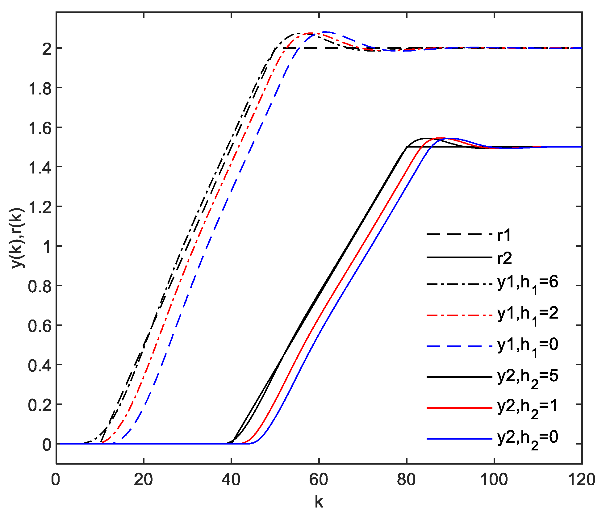
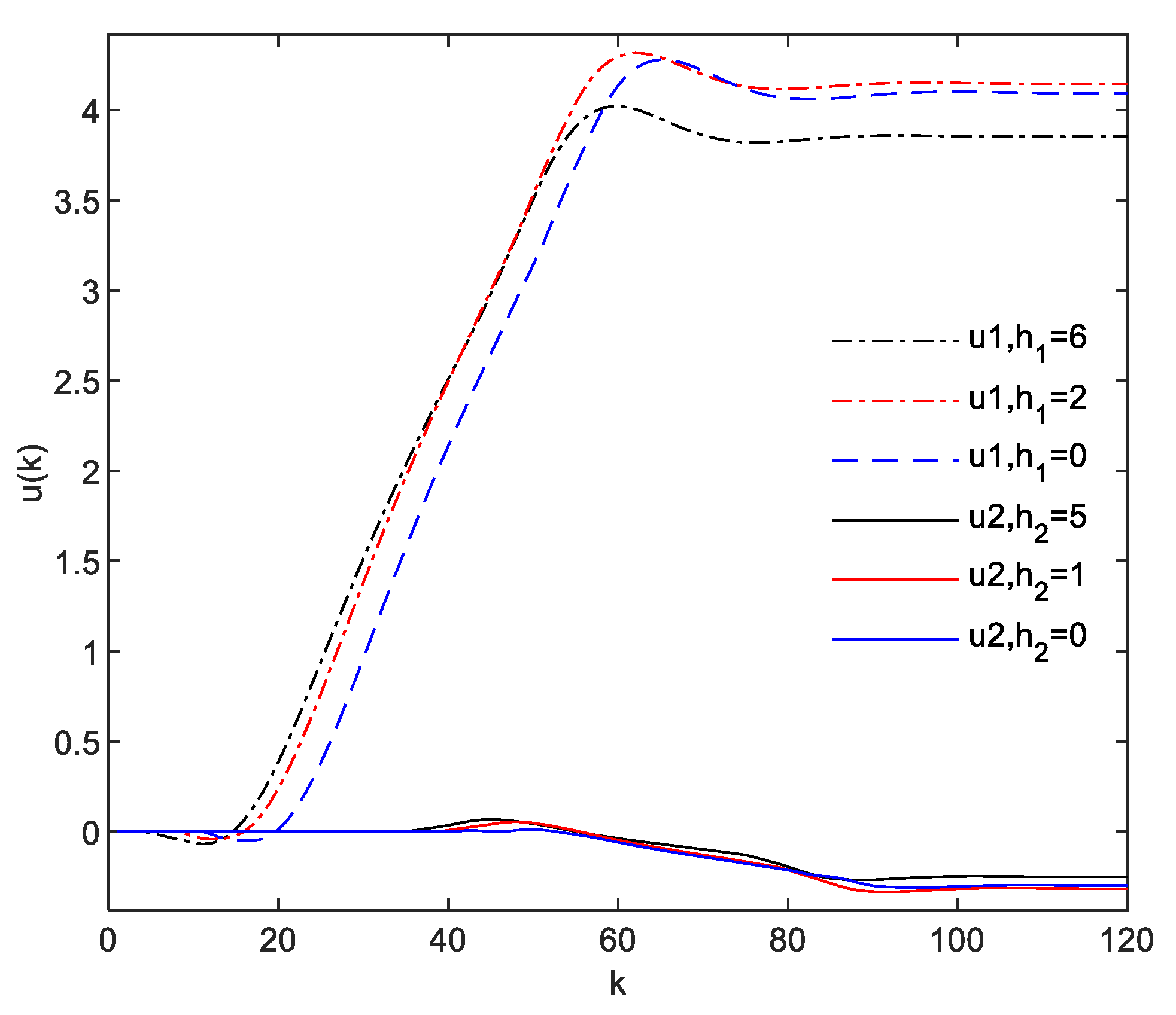
The outputs and the reference signals are depicted in Figure 1. Figure 2 plots the control input. As can be seen in Figure 1 and Figure 2, the existence of the preview compensation accelerated the response speed, which reduced the tracking error.

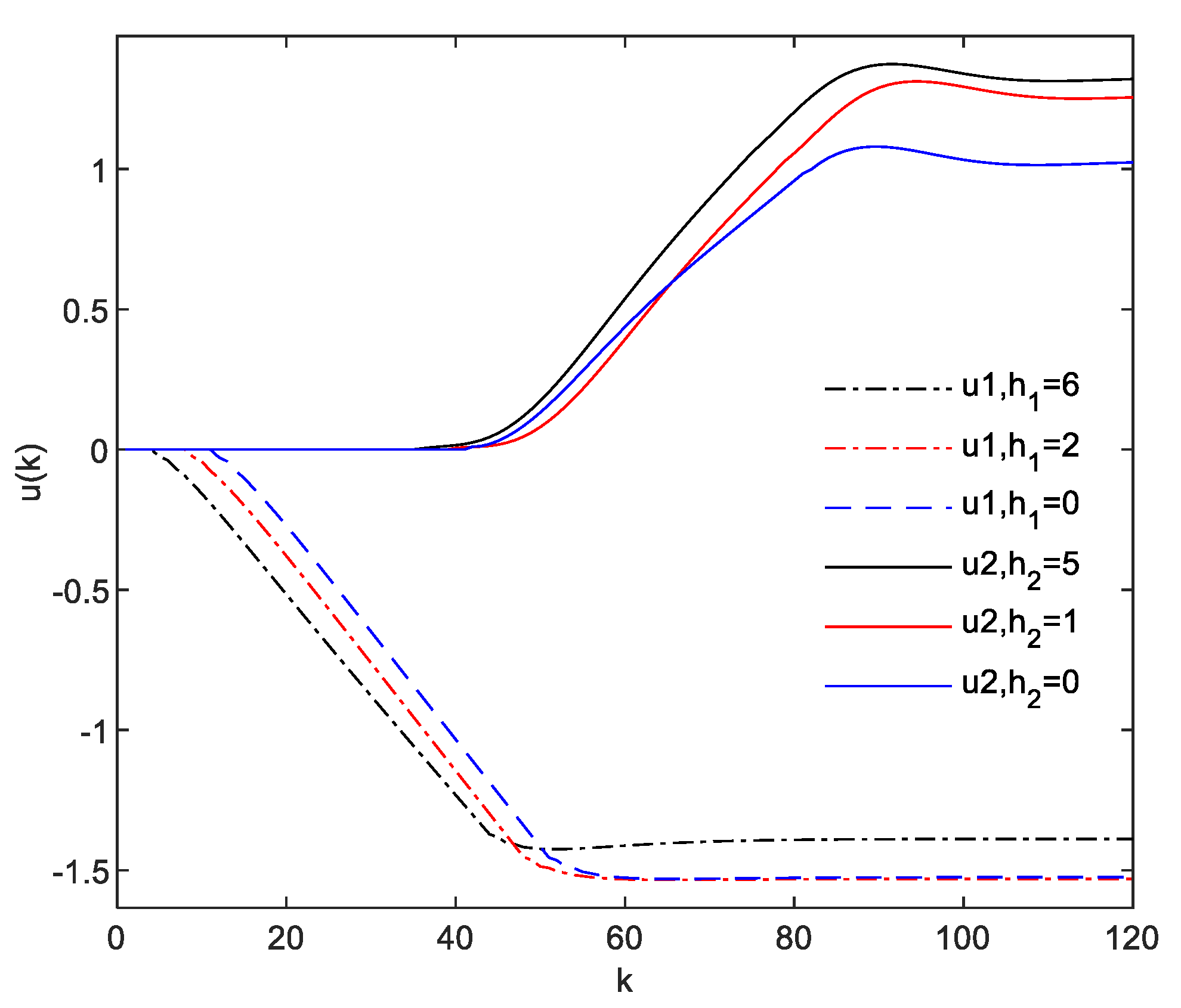
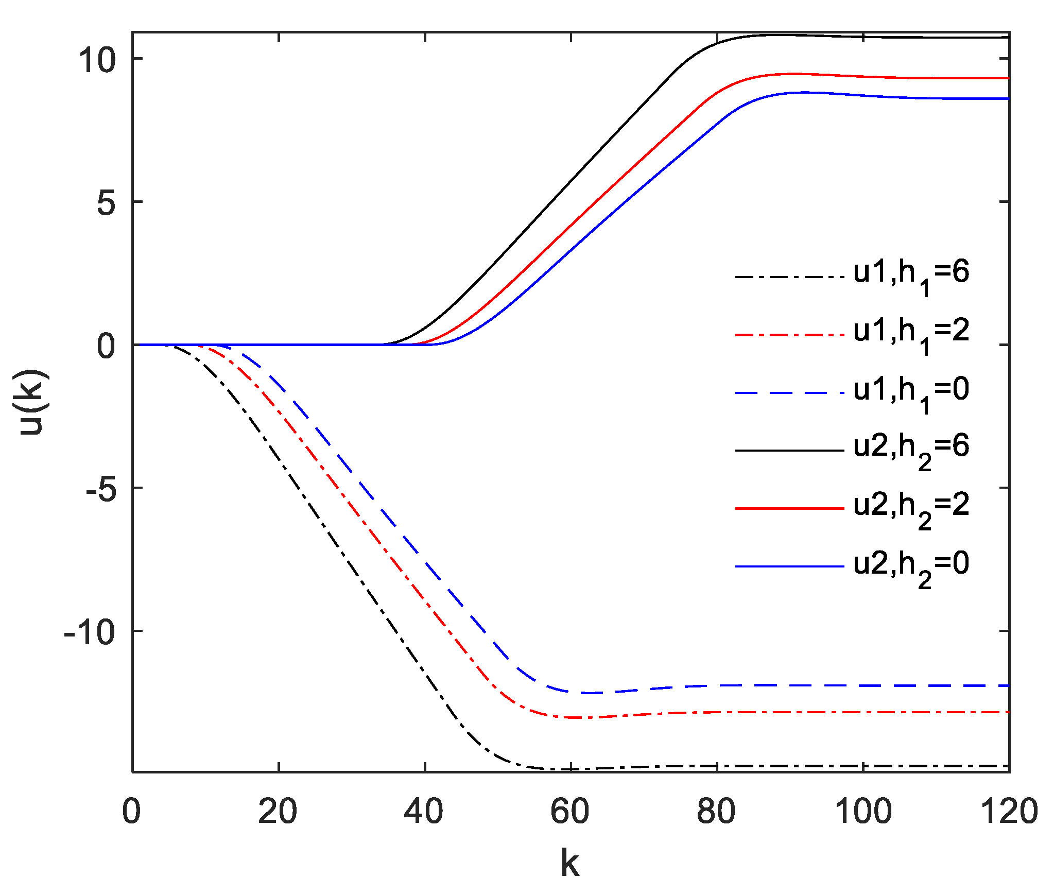
To consider the robustness of the proposed PC, the simulations were completed with different ${\theta }_1$ and ${\theta }_2$ as long as they met A1. Here, the simulation results about ${\theta }_1=1$ and ${\theta }_1=0$ would be given separately. We depicted the output and control input of system (1) with ${\theta }_1=1$ and ${\theta }_2=0$ in Figure 3 and Figure 4. Figure 5 plotted the output of System (1) with ${\theta }_1=0$ and ${\theta }_2=1$. The corresponding input control is shown in Figure 6. One can see from Figure 3, Figure 4, Figure 5 and Figure 6 that the PC made the closed-loop system have a faster dynamic response speed compared with no preview.

The construction methods of AES in [11,13,15,26] were employed, or, equivalently, the future information of $r(k)$ was added to the augmented state vector to derive the AES. For comparison, we performed simulations for this case in [11,13,15,26] by using the same example. From Figure 1 and Figure 7, it can be seen that the future information of the signal components $r_1(k)$ and $r_2(k)$ interacted with each other. This led to poor tracking performance of System (1). In addition, From Figure 1, Figure 2, Figure 7 and Figure 8, we could easily see that our proposed PC provided better tracking performance than those in [11,13,15,26].

Output Feedback Case

In System (1), we let

$$\begin{gathered} A(\theta )=\left[\begin{array}{ccc}1& -0.4& 0.8\\ 1& 0& 0\\ 0& 1& 0\end{array}\right]{\theta }_1+\left[\begin{array}{ccc}1.2& -0.6& 0.7\\ 1& 0& 0\\ 0& 1& 0\end{array}\right]{\theta }_2, \\ B(\theta )=\left[\begin{array}{cc}1& 1\\ 0.3& 0.3\\ 0& 0\end{array}\right]{\theta }_1+\left[\begin{array}{cc}1& 1\\ 1.1& 1\\ 0& 0\end{array}\right]{\theta }_2,C(\theta )={\theta }_1\left[\begin{array}{ccc}1& 0& 0\\ 1& 0& 0\end{array}\right]+{\theta }_2\left[\begin{array}{ccc}1& 0& 0\\ 1& 0& 0\end{array}\right], \\ D(\theta )=0 \end{gathered}$$

Letting ${\alpha }_1={\alpha }_2=4$, ${\beta }_1={\beta }_2=0.6$, and ${\rho }_1={\rho }_2=1$ and ${\gamma }_1=0.3$ and ${\gamma }_2=0.7$, we had matrices $Q_1=6(C_{Z1,1}+C_{Z2,1})$ and $Q_2=6(C_{Z1,2}+C_{Z2,2})$. According to Theorem 4, the static output feedback gain matrices were obtained as follows.

When ${\mathrm{h}}_1={\mathrm{h}}_2=2$, we obtained

$$K_1=\left[\begin{array}{ccccc}1.26358& -0.40042& -1.26358& -1.26358& -1.26358\\ -1.32911& -0.14526& 1.32911& 1.32911& 1.32911\end{array}\right]$$

$$K_2=\left[\begin{array}{ccccc}1.26358& -0.40042& -1.26358& -1.26358& -1.26358\\ -1.32911& -0.14526& 1.32911& 1.32911& 1.32911\end{array}\right]$$

When ${\mathrm{h}}_1={\mathrm{h}}_2=6$, $K_1$ and $K_2$ are given, respectively, by

$$\begin{array}{l}{K}_1=[\begin{array}{cccccc}1.31567& -0.30661& -1.31567& -1.31567& -1.31567& -1.31567\\ -1.38506& -0.24404& 1.38506& 1.38506& 1.38506& 1.38506\end{array}\\ \begin{array}{ccc}-1.31567& -1.31567& -1.31567\\ 1.38506& 1.38506& 1.38506\end{array}],\end{array}$$

$$\begin{array}{l}{K}_2=[\begin{array}{cccccc}1.31567& -0.30661& -1.31567& -1.31567& -1.31567& -1.31567\\ -1.38506& -0.24404& 1.38506& 1.38506& 1.38506& 1.38506\end{array}\\ \begin{array}{ccc}-1.31567& -1.31567& -1.31567\\ 1.38506& 1.38506& 1.38506\end{array}],\end{array}$$

When ${\mathrm{h}}_1={\mathrm{h}}_2=0$, we obtained

$$K_1=\left[\begin{array}{cc}1.18156& -0.45238\\ -1.24364& -0.09158\end{array}\right]$$

$$K_2=\left[\begin{array}{cc}1.18156& -0.45238\\ -1.24364& -0.09158\end{array}\right]$$

For the Signal (52) and (53), Figure 9 depicts the output and the reference Signals (52) and (53). Figure 10 indicates the control input for different preview lengths. From Figure 9 and Figure 10, we found that the output response could reach a steady state faster when using the output controller with preview compensation.

For the static output feedback case, two extreme cases, namely, ${\theta }_1=1$ and ${\theta }_1=0$ have also been considered. Figure 11 and Figure 12, respectively, show the output response and control input of System (1) by static output controller under ${\theta }_1=0$. When ${\theta }_1=1$, Figure 13 and Figure 14 show the response and the control input curves, respectively. It is evident from Figure 11, Figure 12, Figure 13 and Figure 14 that the tracking effect was still remarkable under the reference input preview compensation.

Similarly, for the output feedback case, the simulations were completed when the design methods in [11,13,15,26] were used. From these simulation results, we could find that the proposed output feedback PC had more advantages. Simulation and analysis were made separately under different situations of parameters ${\theta }_1$ and ${\theta }_2$. Considering length limitations, the figures for these results would not be provided here.

6. Conclusions

The PC problem for MIMO discrete-time systems with polytopic uncertainties was discussed in this paper. We derived the AES including previewed information on $r_i(k)$ by using classical difference method. The parameter-dependent state feedback and output feedback were proposed and the conditions of the design methods of PCs were given by using parameter-dependent quadratic Lyaounov functions and LMI approach. The robust controllers with preview actions using LMIs were presented.

References

- Zheng, D.Z. Linear System Theory; Tsinghua University Press: Beijing, China, 2012. [Google Scholar]
- Tan, K.K.; Zhao, S.; Xu, J.X. Online automatic tuning of a proportional integral derivative controller based on an iterative learning control approach. IET Control Theory A 2007, 1, 90–96. [Google Scholar] [CrossRef]
- Li, Y.; Zhao, S.; He, W.; Lu, R. Adaptive finite-time tracking control of full state constrained nonlinear systems with dead-zone. Automatica 2019, 100, 99–107. [Google Scholar] [CrossRef]
- Wang, Y.; Wang, R.; Xie, X.; Zhang, H. Observer-based H∞ fuzzy control for modified repetitive control. Neurocomputing 2018, 286, 141–149. [Google Scholar] [CrossRef]
- Birla, N.; Swarup, A. Optimal preview control: A review. Optim. Control Appl. Methods 2015, 36, 241–268. [Google Scholar] [CrossRef]
- Zhen, Z.Y. Research development in preview control theory and applications. Acta Autom. Sin. 2016, 42, 172–188. [Google Scholar]
- Sheridan, T.B. Three models of preview control. IEEE Trans. Hum. Factors Electron. 1996, 7, 91–102. [Google Scholar] [CrossRef]
- Bender, E.K. Optimum linear preview control with application to vehicle suspension. J. Basic Eng. 1968, 90, 213–221. [Google Scholar] [CrossRef]
- Tomizuka, M. Optimal continuous finite preview problem. IEEE Trans. Autom. Control 1975, 20, 362–365. [Google Scholar] [CrossRef]
- Tomizuka, M. Optimal discrete finite preview problem (Why and how is future information important?). J. Dyn. Syst. ASME 1975, 97, 319–325. [Google Scholar] [CrossRef]
- Katayama, T.; Ohki, T.; Inoue, T.; Kato, T. Design of an optimal controller for a discrete-time system subject to previewable demand. Int. J. Control 1985, 41, 677–699. [Google Scholar] [CrossRef]
- Katayama, T.; Hirono, T. Design of an optimal servomechanism with preview action and its dual problem. Int. J. Control 1987, 45, 407–420. [Google Scholar] [CrossRef]
- Tsuchiya, T.; Egami, T. Digital Preview and Predictive Control; Beijing Science and Technology Press: Beijing, China, 1994. [Google Scholar]
- Wu, J.; Liao, F.; Tomizuka, M. Optimal preview control for a linear continuous-time stochastic control system in finite-time horizon. Int. J. Syst. Sci. 2017, 48, 129–137. [Google Scholar] [CrossRef]
- Wang, D.; Liao, F.; Tomizuka, M. Adaptive preview control for piecewise discrete-time systems using multiple models. Appl. Math. Model 2016, 40, 9932–9946. [Google Scholar] [CrossRef]
- Lu, Y.; Liao, F.; Deng, J.; Pattinson, C. Cooperative optimal preview tracking for linear descriptor multi-agent systems. J. Frankl. Inst. 2019, 356, 908–934. [Google Scholar] [CrossRef] [Green Version]
- Lu, Y.; Liao, F.; Deng, J.; Liu, H. Cooperative global optimal preview tracking control of linear multi-agent systems: An internal model approach. Int. J. Syst. Sci. 2017, 48, 2451–2462. [Google Scholar] [CrossRef] [Green Version]
- Running, K.D.; Martins, N.C. Optimal preview control of Markovian jump linear systems. IEEE Trans. Autom. Control 2009, 54, 2260–2266. [Google Scholar] [CrossRef]
- Liao, F.; Wang, Y.; Lu, Y.; Deng, J. Optimal preview control for a class of linear continuous-time large-scale systems. Trans. Inst. Meas. Control 2018, 40, 4004–4013. [Google Scholar] [CrossRef] [Green Version]
- Bidyadhar, S.; Ogeti, P.S. Optimal preview stator voltage-oriented control of DFIG WECS. IET Gener. Transm. Distrib. 2018, 12, 1004–1013. [Google Scholar]
- Kojima, A. H∞ controller design for preview and delayed systems. IEEE Trans. Autom. Control 2015, 60, 404–419. [Google Scholar] [CrossRef]
- Gershon, E.; Shaked, U. H∞ preview tracking control of retarded state- multiplicative stochastic systems. Int. J. Robust Nonlinear Control 2014, 24, 2119–2135. [Google Scholar] [CrossRef]
- Kristalny, M.; Mirkin, L. On the H2 two-sided model matching problem with preview. IEEE Trans. Autom. Control 2012, 57, 207–212. [Google Scholar] [CrossRef]
- Hamada, Y. Preview feedforward compensation: LMI synthesis and flight simulation. IFAC-Pap. 2016, 49, 397–402. [Google Scholar] [CrossRef]
- Li, L.; Liao, F. Robust preview control for a class of uncertain discrete-time systems with time-varying delay. ISA Trans. 2018, 73, 11–21. [Google Scholar] [CrossRef] [PubMed]
- Li, L.; Yuan, Y. Output feedback preview control for polytopic uncertain discrete-time systems with time-varying delay. Int. J. Robust Nonlinear Control 2019, 29, 2619–2638. [Google Scholar] [CrossRef]
- Shao, Y.-F.; Gao, S.-J. Robust preview control of uncertain discrete systems based on an internal model approach. Sci. Technol. Vis. 2018, 1–3. [Google Scholar] [CrossRef]
- Lan, Y.; Xia, J. Observer based design of preview repetitive control for linear discrete systems. Comput. Integr. Manuf. Syst. 2019, 1–18. [Google Scholar]
- Lan, Y.; Xia, J.; Shi, Y. Robust guaranteed-cost preview repetitive control for polytopic uncertain discrete-time systems. Algorithms 2019, 12, 20. [Google Scholar] [CrossRef] [Green Version]
- Han, K.; Feng, J.; Li, Y.; Li, S. Reduced-order simultaneous state and fault estimator based fault tolerant preview control for discrete-time linear time-invariant systems. IET Control Theory A 2018, 12, 1601–1610. [Google Scholar] [CrossRef]
- Han, K.; Feng, J. Data-driven robust fault tolerant linear quadratic preview control of discrete-time linear systems with completely unknown dynamics. Int. J. Control 2019, 1–11. [Google Scholar] [CrossRef]
- Yu, X.; Liao, F. Preview tracking control for a class of discrete-time Lipschitz non-linear time-delay systems. IMA J. Math. Control Inf. 2019, 36, 849–867. [Google Scholar] [CrossRef]
- Lio, W.H.; Jones, B.L.; Rossiter, J.A. Preview predictive control layer design based upon known wind turbine blade-pitch controllers: MPC layer design based upon known blade-pitch controllers. Wind Energy 2017, 20, 1207–1226. [Google Scholar] [CrossRef] [Green Version]
- Zhao, Y.; Cai, Y.; Song, Q. Energy control of plug-in hybrid electric vehicles using model predictive control with route preview. IEEE/CAA J. Autom. Sin. 2018, 1–8. [Google Scholar] [CrossRef] [Green Version]
- Al Khudir, K.; Halvorsen, G.; Lanari, L.; De Luca, A. Stable torque optimization for redundant robots using a short preview. IEEE Robot. Autom. Lett. 2019, 4, 2046–2053. [Google Scholar] [CrossRef] [Green Version]
- Pak, H.A.; Shieh, R. On mimo optimal preview tracking control for known trajectory models. Optim. Control Appl. Methods 1991, 12, 119–130. [Google Scholar] [CrossRef]
- Li, L.; Liao, F. Parameter-dependent preview control with robust tracking performance. IET Control Theory Appl. 2017, 11, 38–46. [Google Scholar] [CrossRef]
- Chen, Y.; Fei, S.; Li, Y. Stabilization of neutral time-delay systems with actuator saturation via auxiliary time-delay feedback. Automatic 2015, 52, 242–247. [Google Scholar] [CrossRef]
- He, Y.; Wu, M.; She, J.-H. Improved bounded-real-lemma representation and H∞ control of systems with polytopic uncertainties. IEEE Trans. Circuits Syst. II Express Briefs 2005, 52, 380–383. [Google Scholar]
- Chang, X.H.; Zhang, L.; Park, H.P. Robust static output feedback H∞ control for uncertain fuzzy systems. Fuzzy Sets Syst. 2015, 273, 87–104. [Google Scholar] [CrossRef]
Figure 1.
The output response and the reference signals.
Figure 2.
The control input.
Figure 3.
The output response of System (1) with .
Figure 4.
The control input of System (1) with
Figure 5.
The output response of System (1) .
Figure 6.
The control input of System (1) with .
Figure 7.
The output response.
Figure 8.
Figure 9.
The output of System (1) with different .
Figure 10.
The control input of System (1) with different .
Figure 11.
, output response of system (1) with different .
Figure 12.
, control of system (1) with different .
Figure 13.
Figure 14.
, control input of system (1) with different .
© 2020 by the authors. Licensee MDPI, Basel, Switzerland. This article is an open access article distributed under the terms and conditions of the Creative Commons Attribution (CC BY) license (http://creativecommons.org/licenses/by/4.0/).
Share and Cite
MDPI and ACS Style
Li, L.; Liao, F. Preview Control for MIMO Discrete-Time System with Parameter Uncertainty. Mathematics 2020, 8, 756. https://0-doi-org.brum.beds.ac.uk/10.3390/math8050756
AMA Style
Li L, Liao F. Preview Control for MIMO Discrete-Time System with Parameter Uncertainty. Mathematics. 2020; 8(5):756. https://0-doi-org.brum.beds.ac.uk/10.3390/math8050756
Chicago/Turabian StyleLi, Li, and Fucheng Liao. 2020. "Preview Control for MIMO Discrete-Time System with Parameter Uncertainty" Mathematics 8, no. 5: 756. https://0-doi-org.brum.beds.ac.uk/10.3390/math8050756
Note that from the first issue of 2016, this journal uses article numbers instead of page numbers. See further details here.