Random Homogenization in a Domain with Light Concentrated Masses

Abstract

In the paper, we consider an elliptic problem in a domain with singular stochastic perturbation of the density located near the boundary, depending on a small parameter. Using the boundary homogenization methods, we prove the compactness theorem and study the behavior of eigenelements to the initial problem as the small parameter tends to zero.

1. Introduction

Boundary value problems in domains with concentrated masses attracted the attention of scientists at the turn of XIX-th and XX-th centuries. The first mathematical paper [1] devoted to studying this problem was published in 1913. There Krylov considers the problem of vibrations of a string with concentrated masses. A study of the eigenfrequencies of vibrations of a string with a concentrated mass at one point is also given in Appendix to Ch. 2 in [2], including the limit behaviour of solutions as the mass goes to zero or infinity. The paper [3] was the first to consider the problem where the concentrated mass belongs to an $\epsilon$-neighbourhood of an interior point, å being a small parameter that describes the concentration and size of the mass. Another approach was used in [4,5,6]. Oleinik introduced a new basic parameter of a body with concentrated masses, the ratio between the adjoined additional mass and the mass of the whole system. She described local oscillations in the vicinity of the concentrated mass. In [4,5,6], this was done for all dimensions and arbitrary masses. The one-dimensional case with one concentrated mass was studied in [7]. The case of finitely many concentrated masses was considered in [8]. The analogous problem for the elasticity system of equations was studied in [9,10] (see also [11,12,13]). In the papers [14,15] the authors constructed the asymptotic expansions of eigenvalues and eigenfunctions to the problem. The case of a three-dimensional linear stationary elasticity system is considered in [16] (see also [17]). A problem on oscillations of a membrane is analyzed in [18].

Papers [19,20,21,22,23,24] deal with to the asymptotic analysis of vibrations of a body with many small dense inclusions situated periodically along the boundary. Analogous problems are considered in [25,26,27]. The paper [28] is devoted to asymptotic analysis of the problem for a linear stationary elasticity system with non-periodic rapidly alternating boundary conditions and with many concentrated masses near the boundary. A problem on the linear stationary elasticity system in domains with stiff concentrated masses is studied in [29]. Paper [30] (see also [31]) is devoted to a detailed study of the behaviour of the eigenelements of the Laplace operator in a domain with non-periodic “light” concentrated masses. A multi-dimensional problem in a domain with periodic “light” masses is considered in [32] (see also [33]). The authors presented estimates for the rate of convergence of the eigenvalues and eigenfunctions of the given problem to the corresponding eigenvalues and eigenfunctions of the homogenized problem. In the paper [34] one can find non-periodic problem with rapidly changing type of boundary conditions.

In [35,36], the authors studied close problems for complex medium and nonlinear situation modeled transport in porous materials including regions with both high and low diffusivities.

In papers [37,38] the authors constructed complete asymptotic expansions for eigenpairs of two-dimensional spectral problems in domains with periodically situated “light” masses. Some of these results were mentioned in [39,40].

In papers [41,42,43,44,45], the authors studied spectral problems in thick cascade junctions with concentrated masses. There is a complete classification of homogenized spectral problems in such domains, as well as local vibrations of the masses.

In this paper, we consider randomly situated “light” concentrated masses on the boundary and prove the convergence results for the spectrum. It appears that the limit (homogenized) problem is deterministic (non random). Some results were shown in [46].

2. Compactness Theorem

Suppose that D is a bounded domain in ${\mathbb{R}}^n,n\ge 2$ with a sufficiently smooth boundary. We consider a family of boundary value problems depending on the small parameter $\epsilon >0$.

$$\left\{\begin{array}{cc}-\Delta u_{\epsilon }={\rho }_{\epsilon }f\hfill & \mathrm{in}D,\\ u_{\epsilon }=0\hfill & \mathrm{on}\hspace{1em}{\Gamma }_{\epsilon }\cup \gamma \subset \partial D,\\ \epsilon \frac{\partial u_{\epsilon }}{\partial \nu }=g\hfill & \mathrm{on}\hspace{1em}\partial D\backslash ({\Gamma }_{\epsilon }\cup \gamma ),\end{array}\right.$$

(1)

where ${\Gamma }_{\epsilon }$ is a piece of the boundary $\partial D$ of the domain D, having a fine-grained structure with $\epsilon$-scale, and $\gamma$ is a fixed part of the boundary $\partial D$. On this part of the boundary, we set the homogeneous Dirichlet boundary condition. On the remaining part of the boundary we set a Neumann boundary condition with the right-hand side $g\left(x\right)$ independent of the small parameter, and $\nu$ is the outward normal vector to the boundary $\partial D$. Here,

$${\rho }_{\epsilon }\left(x\right)=\left\{\begin{array}{cc}{\epsilon }^{-m}\hfill & \mathrm{in}{B}_{\epsilon },\\ 1\hfill & \mathrm{in}D\backslash \overline{B_{\epsilon }}\end{array}\right.,0<m<2,$$

(2)

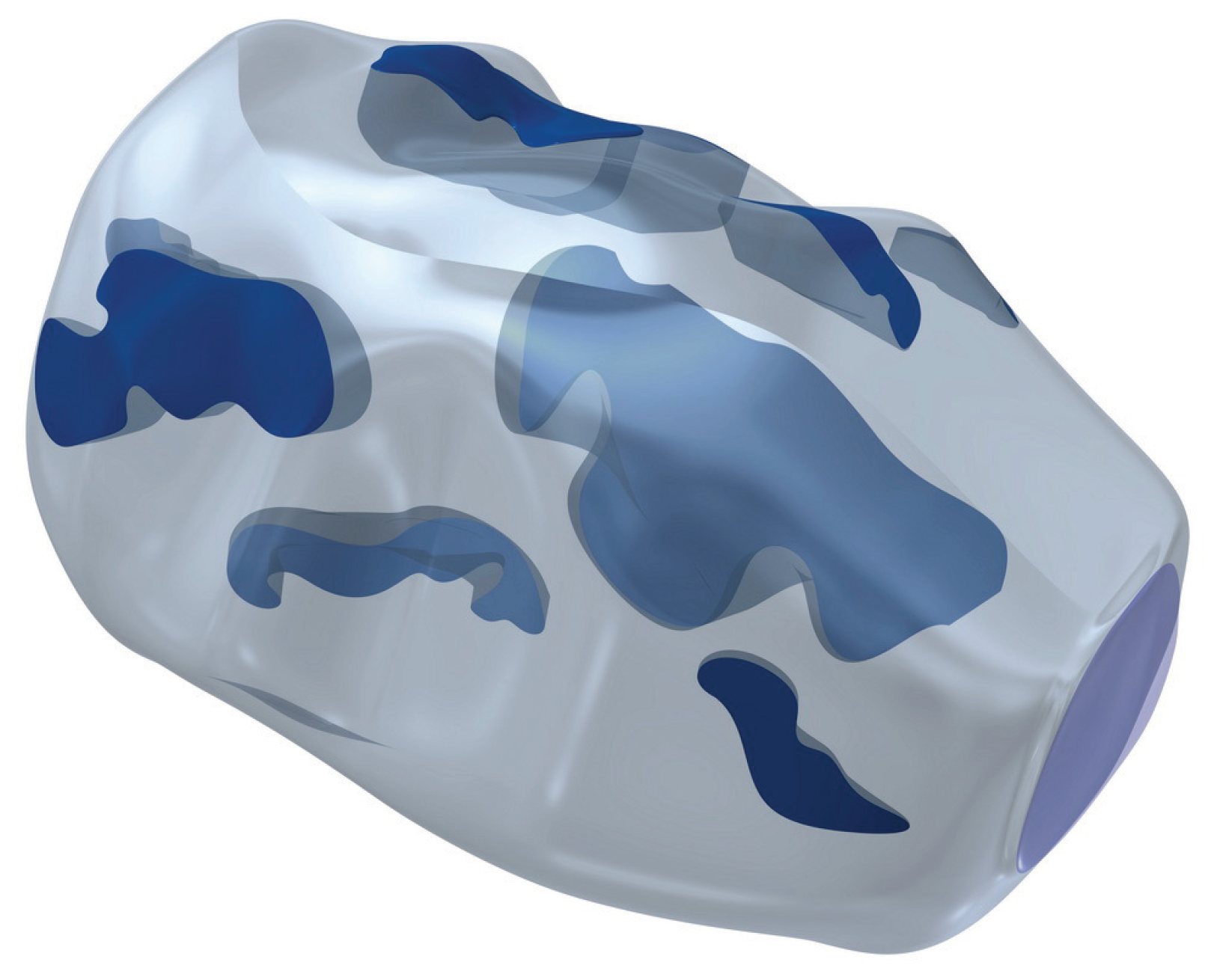
where f is sufficiently smooth function and $B_{\epsilon }$ is a small domain with sufficiently smooth boundary, $\overline{B_{\epsilon }}\cap \partial D={\Gamma }_{\epsilon }$. We assume that the thickness of $B_{\epsilon }$ is of order $\mathcal{O}\left(\epsilon \right)$, i.e., $\mathrm{dist}(x,\partial D)\le \varkappa \epsilon$, if $x\in B_{\epsilon }$, where $\varkappa =const$ (see Figure 1).

Within the paper we use the definition from [47].

Definition 1.

A family of closed sets ${\Gamma }_{\epsilon }\subset \partial D$ we call SELFSIMILAR, if there exist constants $C_1>0$ and $s,1<s\le 2$ independent of ε, such that for any $\epsilon ,0<\epsilon \le {\epsilon }_0$ and for any smooth function $\phi \in C^{\infty }\left(\overline{D}\right)$ with support not intersecting with ${\Gamma }_{\epsilon }$, the following inequality

$${\left(\underset{\partial D}{\int }{\left|\phi \right|}^{s}d{\sigma }_x\right)}^{\frac{1}{s}}\le C_1{\left(\epsilon \underset{D}{\int }{|\nabla \phi |}^{2}dx\right)}^{\frac{1}{2}}$$

(3)

holds true.

We also use the Poincaré and the Friedrichs inequalities in the following form. There exists a constant $C_2$ which only depends on the domain D such that for any function $\phi$ which is continuously differentiable on D the inequality

$$\underset{D}{\int }{\phi }^{2}dx\le C_2\left({\left(\underset{\partial D}{\int }\left|\phi \right|d{\sigma }_x\right)}^2+\underset{D}{\int }{|\nabla \phi |}^{2}dx\right),$$

(4)

holds true, and the inequality

$$\underset{D}{\int }{\phi }^{2}dx\le C_2\underset{D}{\int }{|\nabla \phi |}^{2}dx$$

(5)

holds true whenever $\phi$ also vanishes on $\gamma$.

Our requirements for the smoothness of the boundary $\partial D$ and of the regularity of the set ${\Gamma }_{\epsilon }\subset \partial D$ are necessary only to the extent that the inequalities (3) and (4) are satisfied.

The following asymptotic properties take place.

Theorem 1.

Assume that the family $\left\{{\Gamma }_{\epsilon }\right\}$ is selfsimilar, $g\in L_{s^{\prime }}(\partial D)$, where $s^{\prime }$ is the mutual number to the number s from Definition 1, i.e., $\frac{1}{s}+\frac{1}{s^{\prime }}=1.$ Then

(i) 

the sequence $u_{\epsilon }$, the solutions to problem (1) is bounded in the space $L_s(\partial D)$ as $\epsilon \to 0$;

(ii) 

there exists a measurable function $\mathcal{C}:\partial D\to [0,+\infty )$ and a subsequence ${\epsilon }_k\to 0$ independent of $g\in L_{s^{\prime }}(\partial D)$, such that $u_{{\epsilon }_k}$ weakly converges to $\mathcal{C}\left(x\right)g\left(x\right)$ in $L_s(\partial D)$ as ${\epsilon }_k\to 0$;

(iii) 

the sequence $u_{\epsilon }$ is compact in $L_p\left(D\right),$ where $p<\frac{ns}{n-1}$, and the subsequence $u_{{\epsilon }_k}$ strongly converges in $L_p\left(D\right)$ to the function $u_0$ which satisfies the problem

$$\left\{\begin{array}{cc}-\Delta u_0=f\hfill & inD,\\ u_0=\mathcal{C}g\hfill & on\partial D.\end{array}\right.$$

(6)

Proof. 

To prove (iii) we use the following Lemma from [47].

Lemma 1.

Let D be a domain with a smooth boundary. If the sequence of solutions $v_{\epsilon }$ of the Poisson equation with sufficiently smooth right-hand side in D, is weakly compact in $L_s(\partial D)$, $s>1$. Then it is strongly compact in $L_p\left(D\right)$, $p<\frac{ns}{n-1}$.

Remark 1.

In [47], this statement is proved for a sequence of harmonic functions but the proof can be easily modified for the sequence of solutions to the Poisson equation in D.

Now the statement (iii) follows form this Lemma and both (i), (ii).

To show (i) we write down the integral identity of the problem (1). We have

$$\epsilon \underset{D}{\int }\nabla u_{\epsilon }\nabla vdx=\epsilon \underset{D}{\int }{\rho }_{\epsilon }fvdx+\underset{\partial D}{\int }gvd{\sigma }_x$$

(7)

for any smooth v with compact support in $\overline{D}\backslash {\Gamma }_{\epsilon }$. Denote by $H_0^1(D,{\Gamma }_{\epsilon }\cup \gamma )$ the closure by the Sobolev norm of $W_2^1\left(D\right)$ the set of smooth functions with compact support in $\overline{D}\backslash ({\Gamma }_{\epsilon }\cup \gamma )$. By means of the Lax–Milgram Lemma (see, for instance [48]) applied to the functionals in left- and right-hand sides of (7) on $H_0^1(D,{\Gamma }_{\epsilon }\cup \gamma )$, using (3) and (4), we conclude that there exists a unique solution $u_{\epsilon }\in H_0^1(D,{\Gamma }_{\epsilon }\cup \gamma )$.

Remark 2.

It should be noted, that due to the continuity, the inequalities (3), (4) and (7) are valid for functions from $H_0^1(D,{\Gamma }_{\epsilon }\cup \gamma )$. Moreover, there is a continuous trace operator from $H_0^1(D,{\Gamma }_{\epsilon }\cup \gamma )$ to $L_s(\partial D)$.

Substituting $v=u_{\epsilon }$ in (7), we get

$$\begin{array}{cc}\hfill \epsilon \underset{D}{\int }{|\nabla u_{\epsilon }|}^{2}dx\le & {\left(\underset{\partial D}{\int }{\left|g\right|}^{s^{\prime }}d{\sigma }_x\right)}^{\frac{1}{s^{\prime }}}{\left(\underset{\partial D}{\int }{\left|u_{\epsilon }\right|}^{s}d{\sigma }_x\right)}^{\frac{1}{s}}+\hfill \\ \hfill & +\sqrt{\epsilon \underset{D}{\int }{f}^{2}dx}\sqrt{\epsilon \underset{D}{\int }{u}_{\epsilon }^{2}dx}+{\epsilon }^{1-m}\sqrt{\underset{B_{\epsilon }}{\int }{f}^{2}dx}\sqrt{\underset{B_{\epsilon }}{\int }{u}_{\epsilon }^{2}dx}.\hfill \end{array}$$

(8)

Note that ${\displaystyle \underset{B_{\epsilon }}{\int }{f}^{2}dx=\mathcal{O}\left(\epsilon \right)}$. Using (3), the Friedrichs type inequalities (5) and

$$\underset{B_{\epsilon }}{\int }{u}_{\epsilon }^{2}dx\le K{\epsilon }^2\underset{D}{\int }{|\nabla u_{\epsilon }|}^{2}dx,$$

we deduce the following estimates:

$$\epsilon \underset{D}{\int }|\nabla u_{\epsilon }{|}^{2}dx\le C_3,\underset{\partial D}{\int }{|u_{\epsilon }|}^{s}d{\sigma }_x\le C_3.$$

(9)

here, the constant $C_3$ does not depend on $\epsilon$. Thus, we proved the statement (i).

Let us consider an auxiliary problem (same as problem (1) with $g=1$)

$$\left\{\begin{array}{c}-\Delta w_{\epsilon }={\rho }_{\epsilon }f\mathrm{in}D,\hfill \\ w_{\epsilon }=0\mathrm{on}{\Gamma }_{\epsilon },\hfill \\ \epsilon \frac{\partial w_{\epsilon }}{\partial \nu }=1\mathrm{on}\partial D\backslash {\Gamma }_{\epsilon },\hfill \end{array}\right.$$

(10)

The integral identity of this problem in $H_0^1(D,{\Gamma }_{\epsilon }\cup \gamma )$ has the form

$$\epsilon \underset{D}{\int }\nabla w_{\epsilon }\nabla vdx=\epsilon \underset{D}{\int }{\rho }_{\epsilon }fvdx+\underset{\partial D}{\int }vd{\sigma }_x.$$

(11)

The solution $w_{\epsilon }\in H_0^1(D,{\Gamma }_{\epsilon }\cup \gamma )$ satisfies the bounds analogous to (9), i.e.,

$$\epsilon \underset{D}{\int }|\nabla w_{\epsilon }{|}^{2}dx\le C_4,\underset{\partial D}{\int }{|w_{\epsilon }|}^{s}d{\sigma }_x\le C_4$$

(12)

with the constant $C_4$ independent of $\epsilon$. From (12) we conclude that it is possible to choose a sequence ${\left\{{\epsilon }_k\right\}}_{k\in \mathbb{N}}$ which converges to 0, such that the restrictions of $w_{{\epsilon }_k}$ to $\partial D$ weakly converge in $L_s(\partial D)$. Denote by $\mathcal{C}\left(x\right)$ the limit function on $\partial D$. It is easy to show, that $\mathcal{C}\in L_s(\partial D).$ The nonnegativity of this function follows from the maximum principle for solutions of elliptic equations.

Let us substitute in the identities (7) and (11) $v=\theta w_{\epsilon }$ and $v=\theta u_{\epsilon }$ respectively, where $\theta \in C^{\infty }\left(\overline{D}\right)$ is an arbitrary function. Subtracting these identities from each other, we obtain

$$\epsilon \underset{D}{\int }(w_{\epsilon }\nabla u_{\epsilon }-u_{\epsilon }\nabla w_{\epsilon })\nabla \theta dx=\epsilon \underset{D}{\int }{\rho }_{\epsilon }f\theta (w_{\epsilon }-u_{\epsilon })dx+\underset{\partial D}{\int }(g{w}_{\epsilon }-u_{\epsilon })\theta d{\sigma }_x.$$

(13)

It can be shown that the left-hand side and the first term in the right-hand side of (13) converge to zero as $\epsilon \to 0.$ In fact the boundedness of $\sqrt{\epsilon }{u}_{\epsilon }$ and $\sqrt{\epsilon }{w}_{\epsilon }$ in $W_2^1\left(D\right)$ follow from (9) and (12) and the Poincaré inequality; hence, sequences of these functions of the form $\sqrt{{\epsilon }_k}{u}_{{\epsilon }_k}$ and $\sqrt{{\epsilon }_k}{w}_{{\epsilon }_k}$ are strongly compact in $L_2\left(D\right),$ and converge to zero in the $L_p\left(D\right)$-norm, $p<\frac{ns}{n-1}$. Therefore, the sequence converge to zero in $L_2\left(D\right)$. Thus, in the products under the integrals of the left-hand side of (13) one multiplier is bounded in $L_2\left(D\right)$ as $\epsilon \to 0,$ and another tends to zero, and the first term in the right-hand side also converges to zero, since $m<2$ and the sequences $\sqrt{{\epsilon }_k}{u}_{{\epsilon }_k}$ and $\sqrt{{\epsilon }_k}{w}_{{\epsilon }_k}$ converge to zero.

In the second term of the right-hand side of (13) we pass to the limit as ${\epsilon }_k\to 0$. The function $w_{{\epsilon }_k}$ weakly converges to $\mathcal{C}\left(x\right)$ in $L_s(\partial D).$ The functions $u_{{\epsilon }_k}$ are bounded in $L_s(\partial D)$. Taking a subsequence from the subsequence ${\epsilon }_k$ such that $u_{{\epsilon }_k}$ weakly converges in $L_s(\partial D)$ to some limit function $u_0$ on $\partial D$, and pass to the limit on this subsubsequence. We get

$$\underset{\partial D}{\int }\left(g(x)\mathcal{C}(x)-u_0\left(x\right)\right)\theta \left(x\right)d{\sigma }_x=0.$$

Since $\theta \in C\left(\overline{D}\right)$ is an arbitrary function on $\partial D$, the function $u_0=gC$, i.e., $u_0$ is independent of the choice of the subsubsequence. Therefore, the whole subsequence $u_{{\epsilon }_k}$ has a unique limit. This proves Theorem 1.  □

3. Random Structure

In this section, we describe the structure of micro inhomogeneous sets near the boundary. To describe the family $\left\{{\Gamma }_{\epsilon }\right\}$ in detail we use an approach from [48,49].

3.1. Notation

Let $(\mathsf{\Omega },\mathfrak{B},\mu )$ be a probability space with a semigroup of mappings $T_{\xi }:\mathsf{\Omega }\to \mathsf{\Omega },$ measurable in $\omega \in \mathsf{\Omega },\xi \in {\mathbb{R}}^{n-1}$ and preserving the measure $\mu$ on $\mathsf{\Omega }$. We assume the following group property to be satisfied: for any $\xi ,\eta \in {\mathbb{R}}^{n-1}$ and any $\omega \in \mathsf{\Omega }$

$$T_{\xi }\circ T_{\eta }\omega =T_{\xi +\eta }\omega ,T_0\omega =\omega .$$

Definition 2.

A measurable function $\phi :\mathsf{\Omega }\times {\mathbb{R}}^{n-1}\to \mathbb{R}$ is called a RANDOM STATISTICALLY HOMOGENEOUS, if it has the form $\phi (\omega ,\xi )=\varphi \left(T_{\xi }\omega \right),(\omega ,\xi )\in \mathsf{\Omega }\times {\mathbb{R}}^{n-1})$, where ϕ is a Borel measurable function on ${\mathbb{R}}^{n-1}$.

Definition 3.

A random subset of ${\mathbb{R}}^{n-1}$ is called HOMOGENEOUS, if its indicator function is statistically homogeneous.

The family $T=\{T_{\xi }:\xi \in {\mathbb{R}}^{n-1}\}$ on $\mathsf{\Omega }$ forms an $(n-1)$-dimensional dynamical system. In the further analysis we assume T to be ERGODIC, i.e., any $\mu$-measurable function on $\mathsf{\Omega }$, invariant with respect to this semigroup T, is almost everywhere a constant. Under this assumption, the following Birkhoff theorem holds true (see, for instance, [48,49]).

Theorem 2

(The Birkhoff theorem). For any function $\varphi \in L_{\alpha }\left(\mathsf{\Omega }\right)(\alpha \ge 1)$ and any bounded domain $D\subset {\mathbb{R}}^{n-1}$ we have

$$\underset{\epsilon \to 0}{lim}\frac{1}{|D|}\underset{D}{\int }\varphi \left(T_{\frac{x}{\epsilon }}\omega \right)dx=\underset{\mathsf{\Omega }}{\int }\varphi \left(\omega \right)\mu \left(d\omega \right)\equiv \langle \varphi \rangle$$

almost surely.

Here, we used the notation $\langle ·\rangle$ for the mathematical expectation and $|·|$ for the volume of a domain. From the Birkhoff theorem, one can conclude that the family of functions $\left\{\varphi \left(T_{\frac{x}{\epsilon }}\omega \right):\epsilon >0\right\}$ weakly converges almost surely to $\langle \varphi \rangle$ in $L_{\alpha }^{loc}\left({\mathbb{R}}^{n-1}\right)$ as $\epsilon \to 0$, i.e., for any function $\psi \in L_{\beta }\left({\mathbb{R}}^{n-1}\right)$, $\left(\frac{1}{\alpha }+\frac{1}{\beta }=1\right)$ and any bounded domain $D\subset {\mathbb{R}}^{n-1}$ we have

$$\underset{\epsilon \to 0}{lim}\underset{D}{\int }\varphi \left(T_{\frac{x}{\epsilon }}\omega \right)\psi \left(x\right)dx=\langle \varphi \rangle \underset{D}{\int }\psi \left(x\right)dx$$

for almost all $\omega \in \mathsf{\Omega }$.

3.2. Some Examples

3.2.1. Periodic Case

Let $\mathsf{\Omega }$ be the unit cube $\{\omega \in {\mathbb{R}}^{n-1},0\le {\omega }_j\le 1,j=1,\dots ,n-1\}$. On $\mathsf{\Omega }$ we have a dynamical system $T_{\xi }\omega =\omega +\xi \left(\mathrm{mod}1\right)$. The Lebesque measure is invariant and ergodic due to this dynamical system. The realization of the function $f\left(\omega \right)\in L_{\alpha }\left(\mathsf{\Omega }\right)$ has the form $f(\xi +\omega )$.

3.2.2. Quasi-Periodic Case

Let $\mathsf{\Omega }$ be a unit cube in ${\mathbb{R}}^{n-1}$, $\mu$ be a Lebesque measure on it. For $\xi \in {\mathbb{R}}^m$ we set $T_{\xi }\omega =\omega +\lambda \xi \left(\mathrm{mod}1\right)$, where $\lambda ={\left\{{\lambda }_{ij}\right\}}_{i,j=1}^{n-1}$ is a matrix $m\times (n-1)$. Obviously, the mapping $T_{\xi }$ preserve the measure $\mu$ on $\mathsf{\Omega }$. The dynamical system is ergodic if and only if ${\lambda }_{ij}{k}_j\ne 0$ for any integer vector $k\ne 0$.

Thus, $L_{\alpha }\left(\mathsf{\Omega }\right)$ is the space of periodic functions of d variables, and the realizations have the form $f(\omega +\lambda \xi )$. These realizations are called QUASI-PERIODIC FUNCTIONS, if $f\left(\omega \right)$ is continuous on $\mathsf{\Omega }$.

3.3. Structure of ${\Gamma }_{\epsilon }$

In this subsection, we use the results from [47]. We use statistically homogeneous functions to construct families $\left\{{\Gamma }_{\epsilon }\right\}$ of micro inhomogeneous sets with cellular structure. if $V\left(\omega \right)\in {\mathbb{R}}^{n-1}$ is statistically homogeneous, then its homothetic contractions in $\frac{1}{\epsilon }$ times $\left\{\epsilon V\right(\omega \left)\right\}$ form such a family on $(n-1)$-dimensional manifold $\partial D$. Onwards we use the notation $\epsilon V\left(\omega \right)$ for statistically homogeneous sets in ${\mathbb{R}}^{n-1}$ as well as for sets in ${\mathbb{R}}^n$, defined by $\left\{\right(x,z)\in \partial D,x\in \epsilon V(\omega ),z=0\},$ where x is a local coordinate on $\partial D$, and z is a coordinate along the normal to $\partial D$.

To avoid some simple technical difficulties, we consider $D=\{(x,z),0<x_i<1,0<z<1\},$ and consider the case, when rapidly changing boundary conditions in (1) are set only on one (lower) face of the cube, on other faces we assume homogeneous Dirichlet boundary condition to be satisfied. Thus ${\Gamma }_{\epsilon }=Q\cap \epsilon V\left(\omega \right),$ where $Q=\{(x,z),0<x_i<1,z=0\}$ is the lower face of the cube. Also we denote by $\gamma$ the other faces of the cube $\partial D\backslash Q$.

For having the family $\left\{{\Gamma }_{\epsilon }\right\}$ to be selfsimilar in the sense of Definition 1, we demand the statistically homogeneous set $V\left(\omega \right)$ to satisfy an additional property, which we call nondegeneracy.

Definition 4.

A random statistically homogeneous closed subset $V\left(\omega \right)\subset {\mathbb{R}}^{n-1}$ is called NONDEGENERATE, if there exists a positive statistically homogeneous function $h=h\left(\omega \right)$, such that for almost all ω and for any function $\phi \in C_0^{\infty }\left({\mathbb{R}}^n\backslash V\left(\omega \right)\right)$ with support of φ disjoint from $V\left(\omega \right)$, the following inequality:

$$\underset{{\mathbb{R}}^{n-1}}{\int }h\left(T_x\omega \right){\phi }^2(x,0)dx\le \underset{0}{\overset{\infty }{\int }}\underset{{\mathbb{R}}^{n-1}}{\int }{|\nabla \phi (x,z)|}^{2}dxdz$$

(14)

holds true, wherein

$$\langle h^{-1-\delta }\rangle <+\infty ,$$

(15)

with some $\delta ,0<\delta \le +$.

The non-degeneracy condition of $V\left(\omega \right)$ we use below for studying the auxiliary problem (24). The estimates (14) and (15) guarantee its solvability. In [50] the author used analogous conditions for porous medium.

Assume that $V\left(\omega \right)$ is a union in ${\mathbb{R}}^{n-1}$ of balls with radii ${\rho }_i>0$ centered in isolated points $y_i$. And respectively $B\left(\omega \right)$ is a union in ${\mathbb{R}}^n$ of semiballs ($z>0$) with radii ${\rho }_i>0$ centered in the same isolated points $y_i$. The balls are allowed to intersect (see Figure 2). Denote by $\mathit{r}=r_{\omega }\left(y\right)$ the distance from $y\in {\mathbb{R}}^{n-1}$ to the nearest center $y_i$, $\mathit{\rho }={\rho }_{\omega }\left(y\right)$ is the radius of the ball centered in $y_i$, nearest to y. If $V\left(\omega \right)$ is statistically homogeneous domain, then the random functions $\mathit{r}$ and $\rho$ are also statistically homogeneous.

Let us construct h from (14) using the functions $\mathit{r}$ and $\rho$.

Lemma 2.

The inequality (14) holds true, if

$$h=\frac{1}{\mathit{\rho }}H\left(\frac{\mathit{r}}{\mathit{\rho }}\right),H\left(t\right)=\left\{\begin{array}{cc}\frac{1}{2t^3},\hfill & n=2,\hfill \\ \frac{1}{8t^{3}log(t+1)},\hfill & n=3,\hfill \\ \frac{n-3}{4t^{2n-3}},\hfill & n>3.\hfill \end{array}\right.$$

(16)

Proof. 

We split ${\mathbb{R}}^{n-1}$ into measurable subsets $V_i$, consisting of points for which $y_i$ is the nearest center (see Figure 3). According to our assumption, the set $\left\{y_i\right\}$ has no accumulation points, hence $V_i$ are polyhedra. In each of them we set the polar system of coordinates $(r,\theta ),$ where $r=|y-y_i|$ and $\theta$ are polar angles. Obviously, the polyhedra are starshaped with respect to the center, hence their boundaries are defined in polar coordinates by unique functions $r=R\left(\theta \right).$ Inside the polyhedra the function ${\rho }_{\omega }\left(y\right)$ are equal to the respective constants $\mathit{\rho }>0.$

For any point $M\in V_i$ with coordinates $(\mathit{r},\theta )$, $\mathit{r}>\mathit{\rho },$ we set $\mathit{a}=\frac{{\rho }^2}{\mathit{r}}$ and construct a point $\mathit{M}\in V_i$ with coordinates $(\mathit{a},\theta ),$$0<\mathit{a}<\mathit{\rho }.$ Connect the points M and $\mathit{M}$ by the curve l in the cylinder $V_i\times [0,\infty ),$ which is defined in the cylindrical coordinates $(r,\theta ,z)$ by the equation

$$z=\frac{(\mathit{r}-r)(r-\mathit{a})}{\mathit{r}-\mathit{a}},\theta =const,\mathit{a}\le r\le \mathit{r}.$$

(17)

Consider an arbitrary function $\phi \in C_0^{\infty }\left({\mathbb{R}}^n\backslash V\left(\omega \right)\right)$ with compact support, for which we verify the inequality (14). In each cylinder $V_i\times [0,\infty )$ we have $\phi (r,\theta ,0)\equiv 0$ if $r<\mathit{\rho }.$ We represent the value of $\phi$ in the point $(\mathit{r},\theta ,0),\mathit{r}>\mathit{\rho },$ in the form of the integral over the curve l, i.e.,

$$\phi (\mathit{r},\theta ,0)=\underset{\mathit{a}}{\overset{\mathit{r}}{\int }}\frac{d\phi }{dr}dr,$$

(18)

where $\frac{d\phi }{dr}=\frac{\partial \phi }{\partial r}+\frac{\partial \phi }{\partial z}\frac{dz}{dr}$ is the derivative along the curve $l.$ Obviously, $|\frac{d\phi }{dr}|\le |\nabla \phi |\sqrt{1+{\left(\frac{dz}{dr}\right)}^2}.$ Using the Cauchy–Schwartz–Bunjakovskii inequality, we deduce

$${\phi }^2(\mathit{r},\theta ,0)\le \underset{\mathit{a}}{\overset{\mathit{r}}{\int }}{|\nabla \phi |}^2\left[1+{\left(\frac{dz}{dr}\right)}^2\right]r^{n-2}dr\underset{\mathit{a}}{\overset{\mathit{r}}{\int }}\frac{dt}{t^{n-2}}.$$

(19)

Denote

$$I=I\left(\theta \right)=\underset{\mathit{\rho }}{\overset{R\left(\theta \right)}{\int }}{\phi }^2(\mathit{r},\theta ,0)\frac{1}{\mathit{\rho }}H\left(\frac{\mathit{r}}{\mathit{\rho }}\right){\mathit{r}}^{n-2}d\mathit{r}.$$

Integrating $I\left(\theta \right)$ with respect to the polar angles and taking the summation over all polyhedra $V_i$, we get the left hand side of the inequality (14). Due to (19) we derive the estimate

$$I\le \underset{\mathit{\rho }}{\overset{R\left(\theta \right)}{\int }}\left(\underset{\mathit{a}}{\overset{\mathit{r}}{\int }}\left({|\nabla \phi |}^2\left[1+{\left(\frac{dz}{dr}\right)}^2\right]r^{n-2}\frac{1}{\mathit{\rho }}H\left(\frac{\mathit{r}}{\mathit{\rho }}\right){\mathit{r}}^{n-2}\left(\underset{\mathit{a}}{\overset{\mathit{r}}{\int }}\frac{dt}{t^{n-2}}\right)\right)dr\right)d\mathit{r}.$$

In this estimate we replace the variables $(\mathit{r},r)$ by the variables $(z,r).$ The Jacobian has the form

$$\frac{dz}{d\mathit{r}}=\frac{\mathit{r}{(r-\mathit{a})}^2+\mathit{a}{(\mathit{r}-r)}^2}{\mathit{r}{(\mathit{r}-\mathit{a})}^2}>0.$$

It is easy to prove the following inequalities:

$$1+{\left(\frac{dz}{dr}\right)}^2{|}_{\mathit{a}\le r\le \mathit{r}}\le 2,\frac{dz}{d\mathit{r}}{|}_{\mathit{a}\le r\le \mathit{r}}\ge \frac{\mathit{a}}{\mathit{r}+\mathit{a}}.$$

Thus,

$$I\le 2\underset{\mathit{\rho }}{\overset{R}{\int }}\left(\underset{\mathit{a}}{\overset{\mathit{r}}{\int }}\left({|\nabla \phi |}^2{r}^{n-2}\frac{dz}{d\mathit{r}}\underset{\mathit{r},\mathit{\rho }\le \mathit{r}\le R}{max}\left[\frac{1}{\mathit{\rho }}H\left(\frac{\mathit{r}}{\mathit{\rho }}\right){\mathit{r}}^{n-2}{\left(\frac{\mathit{a}}{\mathit{r}+\mathit{a}}\right)}^{-1}\underset{\mathit{a}}{\overset{\mathit{r}}{\int }}\frac{dt}{t^{n-2}}\right]\right)dr\right)d\mathit{r}.$$

The choice of $H\left(t\right)$ leads to

$$2\underset{\mathit{r},\mathit{\rho }\le \mathit{r}\le R}{max}\left[\frac{1}{\mathit{\rho }}H\left(\frac{\mathit{r}}{\mathit{\rho }}\right){\mathit{r}}^{n-2}{\left(\frac{\mathit{a}}{\mathit{r}+\mathit{a}}\right)}^{-1}\underset{\mathit{a}}{\overset{\mathit{r}}{\int }}\frac{dt}{t^{n-2}}\right]\le 1$$

(20)

for any $\mathit{\rho }$ and R. Keeping in mind (20), replacing the variables $(\mathit{r},r)$ by $(z,r)$ and increasing the domain of integration, we derive

$$I\le \underset{\mathit{\rho }}{\overset{R\left(\theta \right)}{\int }}\left(\underset{\mathit{a}}{\overset{\mathit{r}}{\int }}\left({|\nabla \phi |}^2{r}^{n-2}\frac{dz}{d\mathit{r}}\right)dr\right)d\mathit{r}\le \underset{0}{\overset{\infty }{\int }}\left(\underset{0}{\overset{R\left(\theta \right)}{\int }}{|\nabla \phi |}^2{r}^{n-2}dr\right)dz.$$

Finally, integrating over the polar angles and taking the summation on i, we obtain (14). Lemma is proved. □

4. Deterministic Homogenized Problem

4.1. Statement of the Main Theorem

In this section we give more precise asymptotics of solutions to the problem (1) in the case ${\Gamma }_{\epsilon }\subset \partial D$ is taken as the non-degenerate statistically homogeneous set $V\left(\omega \right)$. In addition, the set $B_{\epsilon }$ is taken as the non-degenerate statistically homogeneous set $B\left(\omega \right)$.

Recall that we consider D, the unit cube with ${\Gamma }_{\epsilon }=Q\cap \epsilon V\left(\omega \right)$, where Q is the lower face of the cube and $\gamma =\partial D\backslash Q$.

The following statement describe the solution of the homogenized problem.

Theorem 3.

Suppose that in Definition 4 $V\left(\omega \right)\subset {\mathbb{R}}^{n-1}$ is a non-degenerate closed subset with $\delta >0$. Then the family $\left\{{\Gamma }_{\epsilon }\right\}$ is selfsimilar with $s=1+\frac{\delta }{(2+\delta )}$ and the solutions $u_{\epsilon }$ to the problem in (1) satisfy the conditions of Theorem 1. In addition the limit function $u_0$ is unique and deterministic (nonrandom). The boundary function $\mathcal{C}\left(x\right)$ does not depend on the choice of the limiting subsequence ${\left\{u_{{\epsilon }_k}\right\}}_{k\in \mathbb{N}}$, it is equal to zero on $\partial D\backslash Q,$ and on Q it is equal to a positive constant.

4.2. Auxiliary Results

Let $({\xi }_1,\dots ,{\xi }_{n-1},\zeta )$ be the Descartes coordinate in ${\mathbb{R}}_{+}^n$ ($\zeta >0$). Denote by $\mathit{S}$ the linear space of those functions $W:\mathsf{\Omega }\times [0,+\infty )\to \mathbb{R},$ with realizations $W(T_x\omega ,\zeta )$ which are smooth functions in ${\mathbb{R}}^n,$ and which together with their derivatives are uniformly bounded in $\omega \in \mathsf{\Omega }$. Moreover, these functions have their support in ${\mathbb{R}}_{+}^n\backslash V\left(\omega \right),$ and are bounded in the $\zeta$-direction.

For non-degenerate domains $V\left(\omega \right)$ the functions from $\mathit{S}$ have the following properties.

Lemma 3.

For any functions $W\in \mathit{S}$ the following estimates

$$\langle W^2(\omega ,0)h\left(\omega \right)\rangle \le \underset{0}{\overset{\infty }{\int }}\langle |\nabla W(T_x\omega ,\zeta ){|}^2\rangle d\zeta ,$$

(21)

$${\left(\langle |W(\omega ,0){|}^t\rangle \right)}^{\frac{1}{t}}\le C\left(t\right){\left(\langle W^2(\omega ,0)h\left(\omega \right)\rangle \right)}^{\frac{1}{2}}$$

(22)

hold true. Here $h\left(\omega \right)$ is a weight–function as in Definition 4, t is a number $1\le t\le s=1+\frac{\delta }{2+\delta },$ and $C\left(t\right)$ is a positive constant, $C\left(1\right)={\langle h^{-1}\rangle }^{\frac{1}{2}}.$

Proof. 

Denote by B and $B_1$ balls in ${\mathbb{R}}^{n-1}$ centered in the same point with radii R and $R(1+r)$, $r>0,$ respectively. Construct smooth cut–off function $\psi \in C_0^{\infty }\left({\mathbb{R}}^{n-1}\right)$ with the support in $B_1$, such that $\psi \equiv 1$ on B, $|\psi |\le 1$, $|\nabla \psi |\le \frac{2}{rR}.$ Substituting $\phi (x,\zeta )=\psi \left(x\right)W(T_x\omega ,\zeta )$, $W\in$$\mathit{S}$, in the inequality (14), we get

$$\underset{B_1}{\int }h\left(T_x\omega \right){\psi }^2\left(x\right)W^2(T_x\omega ,0)dx\le \underset{0}{\overset{\infty }{\int }}\underset{B_1}{\int }|\nabla \left(\psi \left(x\right)W(T_x\omega ,\zeta )\right){|}^{2}dxd\zeta ,$$

which leads to the following estimate:

$$\underset{B}{\int }h\left(T_x\omega \right)W^2(T_x\omega ,0)dx\le \underset{0}{\overset{\infty }{\int }}\underset{B_1}{\int }\left[(1+m)|\nabla W(T_x\omega ,\zeta ){|}^2+{\left(\frac{2}{rR}\right)}^2\left(1+\frac{1}{m}\right)W^2(T_x\omega ,\zeta )\right]dxd\zeta .$$

(23)

here we used the inequality ${(a+b)}^2\le (1+m)a^2+\left(1+\frac{1}{m}\right)b^2$ for an arbitrary $m>0$ and the properties of the cut–off function $\psi .$ Dividing both sides of (23) by the volume of the ball B and passing to the limit as $R\to \infty$, we deduce

$$\langle h(·)W^2(·,0)\rangle \le (1+m){(1+r)}^{n-1}\underset{0}{\overset{\infty }{\int }}\langle |\nabla W(T_x·,\zeta )\rangle d\zeta .$$

According to the ergodic theorem both limits do exist. Then, passing to the limit as m and r go to zero, we obtain (21). The estimate (22) is obtained by means of the Hölder inequality

$${\langle |W(·,0)|}^t{\rangle =\langle |W(·,0)|}^t{h}^{\frac{t}{2}}(·)h^{-\frac{t}{2}}(·)\rangle \le {\langle W^2(·,0)h(·)\rangle }^{\frac{t}{2}}{\langle h^{-\frac{t}{2-t}}(·)\rangle }^{\frac{2-t}{2}}.$$

Keeping in mind that $\frac{t}{2-t}\le 1+\delta ,$ we conclude that the second multiplier in the right–hand side is bounded due to (15). Lemma 3 is proved now. □

Let us consider an auxiliary problem in ${\mathbb{R}}_{+}^n={\mathbb{R}}^{n-1}\times [0,+\infty )$:

$$\left\{\begin{array}{ccc}{\displaystyle \sum _{i=1}^{n-1}}\frac{{\partial }^{2}W}{\partial {\xi }_i^2}+\frac{{\partial }^{2}W}{\partial {\zeta }^2}={\epsilon }^2\rho f\hfill & \mathrm{in}\hfill & {\mathbb{R}}_{+}^n,\hfill \\ W=0\hfill & \mathrm{on}\hfill & V\left(\omega \right),\hfill \\ \frac{\partial W}{\partial \zeta }=-1\hfill & \mathrm{on}\hfill & {\mathbb{R}}^{n-1}\backslash V\left(\omega \right),\hfill \end{array}\right.$$

(24)

where

$$\rho \left(\xi \right)=\left\{\begin{array}{cc}{\epsilon }^{-m}\hfill & \mathrm{in}B,\\ 1\hfill & \mathrm{in}{\mathbb{R}}_{+}^n\backslash \overline{B}\end{array}\right.,0<m<2$$

(25)

The equations and boundary conditions in (24) correspond to the auxiliary problem (10) and formally can be obtained by the change of variables $(x,z)\to (\xi ,\zeta )\equiv \left(\frac{x}{\epsilon },\frac{z}{\epsilon }\right)$. The solution is defined in the closure of $\mathit{S}$ with respect to an appropriate norm.

Note that due to the invariance of the measure $\mu$ with respect to $T_{\xi }$ the right–hand side of (21) does not depend on $\xi$. We take this expression as the square of the new norm. Denote by $\overline{\mathit{S}}$ the completion of $\mathit{S}$ with respect to this new norm. The inequality (22) shows us, that for functions $W\in \overline{\mathit{S}}$ one can define the trace $W(\omega ,0)$, and the trace operator continuously maps $\overline{\mathit{S}}$ to $L_s(\partial \mathsf{\Omega })$.

The realization $W(T_{\xi }\omega ,\zeta )$ of the function $W\in \overline{\mathit{S}},$ we call a solution of the auxiliary problem (24), if it satisfies the integral identity

$$\underset{0}{\overset{\infty }{\int }}\langle \nabla W(T_{\xi }\omega ,\zeta )\nabla \tilde{W}(T_{\xi }\omega ,\zeta )\rangle d\zeta ={\epsilon }^2\underset{0}{\overset{\infty }{\int }}\rho (\xi ,\zeta )f(\epsilon \xi ,\epsilon \zeta )\langle \tilde{W}(T_{\xi }\omega ,\zeta )\rangle d\zeta +\langle \tilde{W}(T_{\xi }\omega ,0)\rangle$$

(26)

for any function $\tilde{W}\in \mathit{S}.$

Due to Lemma 3 the bilinear form and the linear functional in (26) satisfy the conditions of the Lax–Milgram lemma (see, for instance [48]). Thus, the unique solution $W\in \overline{\mathit{S}}$ to the problem (24) does exist. Besides, substituting $\tilde{W}=W$ in (26), applying the Cauchy–Swartz–Bunjakovski inequality, the Friedrichs inequality and (21), we derive the estimate

$$\langle W(\omega ,0)\rangle \le \langle h^{-1}\rangle .$$

(27)

The realization $W(T_{\xi }\omega ,\zeta )$ of the solution to problem (24) does not only satisfy the equation in (26), but also as a function from $W_{loc}^{1,2}\left({\mathbb{R}}_{+}^n\right).$

Lemma 4.

For almost all $\omega \in \mathsf{\Omega }$ the realization $W(T_x\omega ,z)$ of the solution to the problem (24) belongs to $W_{loc}^{1,2}\left({\mathbb{R}}_{+}^n\right)$ and satisfies the integral identity

$$\underset{{\mathbb{R}}_{+}^n}{\int }\nabla W(T_{\xi }\omega ,\zeta )\nabla \psi (\xi ,\zeta )d\xi d\zeta ={\epsilon }^2\underset{{\mathbb{R}}_{+}^n}{\int }\rho (\xi ,\zeta )f(\epsilon \xi ,\epsilon \zeta )\psi (\xi ,\zeta )d\xi d\zeta +\underset{{\mathbb{R}}^{n-1}}{\int }\psi (\xi ,0)d\xi$$

(28)

for sufficiently small ε and any smooth function $\psi (x,z)$ with compact support in ${\mathbb{R}}_{+}^n\backslash V\left(\omega \right).$

The proof can be found in [49] (see also [47]).

We use the identity (28) in modified form

$$\epsilon \underset{{\mathbb{R}}_{+}^n}{\int }\nabla W\left(T_{\frac{x}{\epsilon }}\omega ,\frac{z}{\epsilon }\right)\nabla v(x,z)dxdz=\epsilon \underset{{\mathbb{R}}_{+}^n}{\int }{\rho }_{\epsilon }(x,z)f(x,z)v(x,z)dxdz+\underset{{\mathbb{R}}^{n-1}}{\int }v(x,0)dx.$$

(29)

here $v(x,z)$ is a smooth function with compact support in ${\mathbb{R}}_{+}^n\backslash \epsilon V\left(\omega \right).$ The identity (29) is obtained from (28) by scaling of the coordinates.

4.3. Proof of Theorem 3

Proof. 

Let us prove the selfsimilarity of the family $\left\{{\Gamma }_{\epsilon }\right\}.$ Consider a smooth function $\phi$ in $\overline{D}$ with its support in $\overline{D}\backslash ({\Gamma }_{\epsilon }\cup \gamma ).$ Assume that $s=1+\frac{\delta }{(2+\delta )}$, $\alpha =\frac{2}{s}$, $\beta =\frac{2}{2-s}\left(\frac{1}{\alpha }+\frac{1}{\beta }=1\right).$ Using the Hölder inequality, we get

$$\underset{Q}{\int }{|\phi |}^{s}dx\le {\left(\underset{Q}{\int }h\left(T_{\frac{x}{\epsilon }}\omega \right){|\phi |}^{2}dx\right)}^{\frac{1}{\alpha }}{\left(\underset{Q}{\int }{h}^{-\frac{\beta }{\alpha }}\left(T_{\frac{x}{\epsilon }}\omega \right)dx\right)}^{\frac{1}{\beta }},$$

(30)

where Q is the lower face of the cube D, and $h\left(\omega \right)$ is the weight–function from the definition (19).

Changing variables $(x,z)\to (\frac{x}{\epsilon },\frac{z}{\epsilon })$ in the inequality (14), we estimate the first multiplier in the right–hand side of (30) by the integral over the cube D. We have

$$\underset{Q}{\int }h\left(T_{\frac{x}{\epsilon }}\omega \right){\phi }^2(x,0)dx\le \epsilon \underset{D}{\int }{|\nabla \phi |}^{2}dxdz.$$

Due to the Birkhoff theorem the second multiplier has almost surely the finite limit ${\langle h^{-(1+\delta )}\rangle }^{\frac{1}{\beta }},$ since $\frac{\beta }{\alpha }=1+\delta .$ Thus (30) leads to the inequality (3). Hence, the family $\left\{{\Gamma }_{\epsilon }\right\}$ is almost surely selfsimilar, and for the solutions $u_{\epsilon }$ satisfies the conditions of the Theorem 1.

The boundary function $\mathcal{C}\left(x\right)$ is the limit for the solutions $w_{\epsilon }$ of the auxiliary problem (10). Under the conditions of the Theorem 3 $w_{\epsilon }=0$ on $\gamma$, hence $\mathcal{C}\left(x\right)\equiv 0$ on the faces of D, except Q, independent of the choice of the subsequence ${\epsilon }_k\to 0.$ Let us show, that on Q the boundary function $\mathcal{C}\left(x\right)$ is defined uniquely and is equal to a positive nonrandom constant.

Suppose $\theta \in C^{\infty }\left(\overline{D}\right)$ is a smooth function in the cube D with its support contained in $D\cup Q$, i.e., $\theta \equiv 0$ on all faces of the cube, except Q.

Substituting $v=\theta (x,z)w_{\epsilon }(x,z)$ in the identity (29), where $w_{\epsilon }$ is a solution of the problem (10), and $v=\theta (x,z)W\left(T_{\frac{x}{\epsilon }}\omega ,\frac{z}{\epsilon }\right)$ in the identity (11), subtracting them from each other, we deduce

$$\epsilon \underset{D}{\int }\left[w_{\epsilon }(x,z)\nabla W\left(T_{\frac{x}{\epsilon }}\omega ,\frac{z}{\epsilon }\right)-W\left(T_{\frac{x}{\epsilon }}\omega ,\frac{z}{\epsilon }\right)\nabla w_{\epsilon }(x,z)\right]\theta (x,z)dxdz=$$

$$=\epsilon \underset{D}{\int }{\rho }_{\epsilon }(x,z)f(x,z)\theta (x,z)\left(w_{\epsilon }(x,z)-W\left(T_{\frac{x}{\epsilon }}\omega ,\frac{z}{\epsilon }\right)\right)dxdz+\underset{Q}{\int }\left(w_{\epsilon }(x,0)-W\left(T_{\frac{x}{\epsilon }}\omega ,\frac{z}{\epsilon }\right)\right)\theta (x,0)dx.$$

Passing to the limit as $\epsilon \to 0$, we conclude that the left-hand side and the first term in the right–hand side converge to zero as we have got in (13) (see the proof of Theorem 1). Now let us study the behavior of the second term in the right-hand side. The function $W(T_{\frac{x}{\epsilon }}\omega ,0)$ weakly converges to $\langle W(\omega ,0)\rangle$ in $L_s\left(Q\right)$ due to the ergodicity, and the function $w_{\epsilon }(x,0)$ converges to $\mathcal{C}\left(x\right)$ on some subsequence ${\epsilon }_k\to 0$ due to Theorem 1. The function $\theta (x,z)$ has been chosen arbitrarily on Q, hence $\mathcal{C}\left(x\right)\equiv \langle W(·,0)\rangle$ independently of the choice of the subsequence. Consequently, the whole sequence $w_{\epsilon }(x,0)$ on Q converges to this nonrandom limit. Finally, substituting $\tilde{W}=W$ in the identity (26), we get $\langle W(·,0)\rangle \ge 0.$ Moreover, $\langle W(·,0)\rangle =0$ in the case, when $V\left(\omega \right)$ almost surely coincides with ${\mathbb{R}}^{n-1}.$ The function $\mathcal{C}\left(x\right)$ satisfies the estimate (27).

Theorem 3 is proved. □

5. Convergence of the Spectrum

In this section, we use the approach from [51] to the spectral problem associated with the boundary–value problem (1) with $g\equiv 0$. We consider the following spectral problems:

$$\left\{\begin{array}{cc}\hfill {\displaystyle \Delta \left(u_{\epsilon }^k\right)+{\lambda }_{\epsilon }^k{\rho }_{\epsilon }{u}_{\epsilon }^k}=0& \mathrm{in}D,\hfill \\ \hfill u_{\epsilon }^k=0& \mathrm{on}{\Gamma }_{\epsilon }\cup \gamma ,\hfill \\ \hfill {\displaystyle \frac{\partial u_{\epsilon }^k}{\partial \nu }}=0& \mathrm{on}\partial D\backslash ({\Gamma }_{\epsilon }\cup \gamma ),k=1,2\dots \hfill \end{array}\right.$$

(31)

and

$$\left\{\begin{array}{cc}\hfill {\displaystyle \Delta \left(u^k\right)+{\lambda }_0^k{u}^k}=0& \hfill \mathrm{in}D,\\ \hfill u^k=0& \hfill \mathrm{on}\partial D,k=1,2\dots \end{array}\right.$$

(32)

here, $u_{\epsilon }^k\in H_0^1(D,{\Gamma }_{\epsilon }\cup \gamma ),u^k\in H_0^1\left(D\right),k=1,2,\dots$ are orthogonal bases in $L^2\left(D\right)$. The sets $\left\{{\lambda }_{\epsilon }^k\right\},\left\{{\lambda }_0^k\right\},k=1,2,\dots$ are the corresponding eigenvalues such that

$$0<{\lambda }_{\epsilon }^1\le {\lambda }_{\epsilon }^2\le \dots \le {\lambda }_{\epsilon }^k\le \dots ,0\le {\lambda }_0^1\le {\lambda }_0^2\le \dots \le {\lambda }_0^k\le \dots$$

and they repeat with respect to their multiplicities.

For the sake of completeness, we state here the results on spectral convergence for positive, selfadjoint and compact operators on Hilbert spaces (see [51], Section 3.1, for the proof).

Theorem 4.

Let ${\mathit{H}}_{\epsilon }$ and ${\mathit{H}}_{\mathbf{0}}$ be two separable Hilbert spaces with the scalar products ${(·,·)}_{\epsilon }$ and ${(·,·)}_0$, respectively. Let ${\mathit{A}}_{\epsilon }\in \mathcal{L}\left({\mathit{H}}_{\epsilon }\right)$ and ${\mathit{A}}_{\mathbf{0}}\in \mathcal{L}\left({\mathit{H}}_{\mathbf{0}}\right)$. Let $\mathit{V}$ be a linear subspace of ${\mathit{H}}_{\mathbf{0}}$ such that $\{v:v={\mathit{A}}_{\mathbf{0}}u,u\in {\mathit{H}}_{\mathbf{0}}\}\subset \mathit{V}$. We assume that the following properties are satisfied:

• $C1$ There exists ${\mathit{R}}_{\epsilon }\in \mathcal{L}({\mathit{H}}_{\mathbf{0}},{\mathit{H}}_{\epsilon })$ such that ${({\mathit{R}}_{\epsilon }F,{\mathit{R}}_{\epsilon }F)}_{{\mathit{H}}_{\epsilon }}{\displaystyle \stackrel{\hspace{1em} \epsilon \to 0 \hspace{1em}}{⟶}}{\varkappa }_0{(F,F)}_{{\mathit{H}}_{\mathbf{0}}}$, for all $F\in \mathit{V}$ and certain positive constant ${\varkappa }_0$.
• $C2$ The operators ${\mathit{A}}_{\epsilon }$ and ${\mathit{A}}_{\mathbf{0}}$ are positive, compact and selfadjoint. Moreover, $\parallel {\mathit{A}}_{\epsilon }{\parallel }_{\mathcal{L}\left({\mathit{H}}_{\epsilon }\right)}$ are bounded by a constant, independent of ε.
• $C3$$\parallel {\mathit{A}}_{\epsilon }{\mathit{R}}_{\epsilon }F-{\mathit{R}}_{\epsilon }{\mathit{A}}_{\mathbf{0}}{F\parallel }_{{\mathit{H}}_{\epsilon }}{\displaystyle \stackrel{\hspace{1em} \epsilon \to 0 \hspace{1em}}{\to }}0$ for all $F\in \mathit{V}.$
• $C4$ The family of operators ${\mathit{A}}_{\epsilon }$ is uniformly compact, i.e., for any sequence $F^{\epsilon }$ in ${\mathit{H}}_{\epsilon }$ such that ${sup}_{\epsilon }{\parallel F^{\epsilon }\parallel }_{{\mathit{H}}_{\epsilon }}$ is bounded by a constant independent of ε, we can extract a subsequence $F^{{\epsilon }^{\prime }}$, that verifies the following:

  $$\parallel {\mathit{A}}_{{\epsilon }^{\prime }}{F}^{{\epsilon }^{\prime }}-{\mathit{R}}_{{\epsilon }^{\prime }}{v}^0{\parallel }_{{\mathit{H}}_{{\epsilon }^{\prime }}}\to 0,$$

  as ${\epsilon }^{\prime }\to 0,$ for certain $v^0\in {\mathit{H}}_{\mathbf{0}}$.

Let ${\left\{{\mu }_i^{\epsilon }\right\}}_{i=1}^{\infty }$ and ${\left\{{\mu }_i^0\right\}}_{i=1}^{\infty }$ be the sequences of the eigenvalues of ${\mathit{A}}_{\epsilon }$ and ${\mathit{A}}_{\mathbf{0}}$, respectively, with the classical convention of repeated eigenvalues. Let ${\left\{w_i^{\epsilon }\right\}}_{i=1}^{\infty }$ and (${\left\{w_i^0\right\}}_{i=1}^{\infty }$, respectively) be the corresponding eigenfunctions in ${\mathit{H}}_{\epsilon }$, which are assumed to be orthonormal (${\mathit{H}}_{\mathbf{0}}$, respectively).

Then, for each k, there exists a constant $C_8^k$, independent of ε, such that

$$|{\mu }_k^{\epsilon }-{\mu }_k^0|\le C_8^k\underset{\genfrac{}{}{0pt}{}{u\in \mathcal{N}({\mu }_0^k,{\mathit{A}}_{\mathbf{0}}),}{{\parallel u\parallel }_{{\mathit{H}}_{\mathbf{0}}}=1}}{sup}{\parallel {\mathit{A}}_{\epsilon }{\mathit{R}}_{\epsilon }u-{\mathit{R}}_{\epsilon }{\mathit{A}}_{\mathbf{0}}u\parallel }_{{\mathit{H}}_{\epsilon }},$$

where $\mathcal{N}({\mu }_0^k,{\mathit{A}}_{\mathbf{0}})=\{u\in {\mathit{H}}_{\mathbf{0}},{\mathit{A}}_{\mathbf{0}}u={\mu }_0^{k}u\}$. Moreover, if ${\mu }_k^0$ has multiplicity s (${\mu }_k^0={\mu }_{k+1}^0=\cdots ={\mu }_{k+s-1}^0$), then for any w eigenfunction associated with ${\mu }_k^0$, with ${\parallel w\parallel }_{{\mathit{H}}_{\mathbf{0}}}=1$, there exists a linear combination $w^{\epsilon }$ of eigenfunctions of ${\mathit{A}}_{\epsilon }$, ${\left\{w_j^{\epsilon }\right\}}_{j=k}^{j=k+s-1}$ associated with ${\left\{{\mu }_j^{\epsilon }\right\}}_{j=k}^{j=k+s-1}$ such that

$$\parallel w^{\epsilon }-{\mathit{R}}_{\epsilon }{w\parallel }_{{\mathit{H}}_{\epsilon }}\le C_9^k{\parallel {\mathit{A}}_{\epsilon }{\mathit{R}}_{\epsilon }w-{\mathit{R}}_{\epsilon }{\mathit{A}}_{\mathbf{0}}w\parallel }_{{\mathit{H}}_{\epsilon }},$$

where the constant $C_9^k$ is independent on ε.

We denote by ${\mathit{H}}_{\epsilon }$ the weighted space $L_{2,{\rho }_{\epsilon }}\left(D\right)$ with the scalar product

$${(f^{\epsilon },g^{\epsilon })}_{{\mathit{H}}_{\epsilon }}\equiv \underset{D}{\int }{\rho }_{\epsilon }\left(x\right)f^{\epsilon }\left(x\right)g^{\epsilon }\left(x\right)dx.$$

We denote by ${\mathit{H}}_{\mathbf{0}}$ the space $L_2\left(D\right)$, the scalar product being

$${(f^0,g^0)}_{{\mathit{H}}_{\mathbf{0}}}\equiv \underset{D}{\int }{f}^0{g}^{0}dx.$$

We define the operator

$${\mathit{A}}_{\epsilon }:L_{2,{\rho }_{\epsilon }}\left(D\right)\to H_0^1(D,{\Gamma }_{\epsilon }\cup \gamma ),{\mathit{A}}_{\epsilon }f=u_{\epsilon },$$

where $u_{\epsilon }$ is the solution of problem

$$\left\{\begin{array}{cccc}\hfill -\Delta u_{\epsilon }& =& {\rho }_{\epsilon }f& \mathrm{in}D,\hfill \\ \hfill u_{\epsilon }& =& 0& \mathrm{on}{\Gamma }_{\epsilon }\cup \gamma ,\hfill \\ \hfill {\displaystyle \frac{\partial u_{\epsilon }}{\partial \nu }}& =& 0& \mathrm{on}\partial D\backslash ({\Gamma }_{\epsilon }\cup \gamma ).\hfill \end{array}\right.$$

(33)

We define the operator

$${\mathit{A}}_{\mathbf{0}}:L_2\left(D\right)\to H_0^1\left(D\right),{\mathit{A}}_{\mathbf{0}}f=u,$$

where u is the solution of problem

$$\left\{\begin{array}{cccc}\hfill -\Delta u_0& =& f& \mathrm{in}D,\hfill \\ \hfill u_0& =& 0& \mathrm{on}\partial D.\hfill \end{array}\right.$$

(34)

In fact, ${\mathit{A}}_{\epsilon }$ and ${\mathit{A}}_{\mathbf{0}}$ are operators associated with the eigenvalue problems (31) and (32), respectively.

Now, considering the operators ${\mathit{A}}_{\epsilon }:{\mathit{H}}_{\epsilon }\to {\mathit{H}}_{\epsilon }$ and ${\mathit{A}}_{\mathbf{0}}:{\mathit{H}}_{\mathbf{0}}\to {\mathit{H}}_{\mathbf{0}}$, it is easy to establish the positiveness, self–adjointness and compactness of the operators ${\mathit{A}}_{\epsilon }$ and ${\mathit{A}}_{\mathbf{0}}$, respectively. In particular, the compactness of both operators follows from the compactness of the imbedding of $H^1\left(D\right)$ into the space $L_2\left(D\right).$

Let $\mathit{V}$ be $H_0^1\left(D\right)$, which satisfies $Im{\mathit{A}}_{\mathbf{0}}\subseteq \mathit{V}\subset {\mathit{H}}_{\mathbf{0}}$, and let ${\mathit{R}}_{\epsilon }:L_2\left(D\right)\to L_{2,{\rho }_{\epsilon }}\left(D\right)$ be the operator ${\mathit{R}}_{\epsilon }f=f(1-{\chi }_{\epsilon })$, where ${\chi }_{\epsilon }$ is the indicator function of $B_{\epsilon }$.

Let us verify the conditions $C1-C4$ of Theorem 4 (Theorem 1.4 from [51], Section 3.1).

$C1$. Obviously,

$${({\mathit{R}}_{\epsilon }F,{\mathit{R}}_{\epsilon }F)}_{{\mathit{H}}_{\epsilon }}=\underset{D\backslash B_{\epsilon }}{\int }{F}^{2}dx⟶\underset{D}{\int }{F}^{2}dx={(F,F)}_{{\mathit{H}}_{\mathbf{0}}}$$

as $\epsilon \to 0$. Hence, we conclude that this condition is fulfilled with ${\varkappa }_0=1.$

Let us prove that norms $\parallel {\mathit{A}}_{\epsilon }{\parallel }_{\mathcal{L}\left({\mathit{H}}_{\epsilon }\right)}$ are uniformly bounded with respect to $\epsilon .$ Keeping in mind the equivalence of norms and using the Friedrichs inequalities, we obtain

$$\parallel {\mathit{A}}_{\epsilon }{f\parallel }_{{\mathit{H}}_{\epsilon }}^2=\underset{D}{\int }{u}_{\epsilon }^2\left(x\right){\rho }_{\epsilon }\left(x\right)dx\le C_{10}\parallel u_{\epsilon }{\parallel }_{H^1\left(D\right)}^2\le C_{11}{\parallel f\parallel }_{{\mathit{H}}_{\epsilon }}^2.$$

(35)

Thus, $\parallel {\mathit{A}}_{\epsilon }{f\parallel }_{{\mathit{H}}_{\epsilon }}\le C_{12}{\parallel f\parallel }_{{\mathit{H}}_{\epsilon }}$ holds true and Condition $C2$ is fulfilled.

By Theorem 3 Condition $C3$ is satisfied. Let us consider this condition in more detail. Using the definitions of the operators ${\mathit{A}}_{\epsilon }$, ${\mathit{A}}_{\mathbf{0}}$ for any $f\in \mathit{V}$ and applying the Friedrichs inequality for $B_{\epsilon }$, we have

$$\parallel {\mathit{A}}_{\epsilon }{\mathit{R}}_{\epsilon }f-{\mathit{R}}_{\epsilon }{\mathit{A}}_{\mathbf{0}}{f\parallel }_{{\mathit{H}}_{\epsilon }}^2=\underset{B_{\epsilon }}{\int }{\rho }_{\epsilon }\left(x\right)u_{\epsilon }^2\left(x\right)dx\le {\epsilon }^{2-m}\underset{B_{\epsilon }}{\int }{|\nabla u_{\epsilon }|}^{2}dx⟶0\mathrm{as}\epsilon \to 0.$$

Thus, Condition $C3$ is valid.

Let us verify the last condition, $C4$. If a sequence $\left\{f_{\epsilon }\right\}$ is bounded in ${\mathit{H}}_{\epsilon }$, then by standard arguments we deduce that the solutions ${\{u_{\epsilon }={\mathit{A}}_{\epsilon }{f}_{\epsilon }\}}_{\epsilon }$ to the problem (33) are uniformly bounded with respect to $\epsilon$ in $H^1\left(D\right).$ Therefore, there exists $w\in H^1\left(D\right)$ and a subsequence ${\epsilon }^{\prime }\to 0$ such that $u_{{\epsilon }^{\prime }}\to w$ in $L^2\left(D\right)$ and weakly in $H^1\left(D\right)$. Thus,

$$\parallel {\mathit{A}}_{\epsilon }{f}_{\epsilon }-{\mathit{R}}_{\epsilon }{w\parallel }_{{\mathit{H}}_{\epsilon }}^2=\underset{D}{\int }{(u_{\epsilon }\left(x\right)-w\left(x\right))}^{2}dx$$

and, then, we obtain that:

$$\parallel {\mathit{A}}_{{\epsilon }^{\prime }}{f}_{{\epsilon }^{\prime }}-{\mathit{R}}_{{\epsilon }^{\prime }}{w\parallel }_{{\mathit{H}}_{{\epsilon }^{\prime }}}\to 0\mathrm{as}{\epsilon }^{\prime }\to 0,$$

and Condition $C4$ is fulfilled.

Now, we consider the spectral problems:

$${\mathit{A}}_{\epsilon }{u}_{\epsilon }^k={\mu }_{\epsilon }^k{u}_{\epsilon }^k,u_{\epsilon }^k\in {\mathit{H}}_{\epsilon },$$

$${\mu }_{\epsilon }^1\ge {\mu }_{\epsilon }^2\ge \dots \ge {\mu }_{\epsilon }^k\ge \cdots >0,k=1,2,\dots ,$$

$${(u_{\epsilon }^l,u_{\epsilon }^k)}_{{\mathit{H}}_{\epsilon }}={\delta }_{lk}$$

and

$${\mathit{A}}_{\mathbf{0}}{u}_0^k={\mu }_0^k{u}_0^k,u_0^k\in {\mathit{H}}_{\mathbf{0}},$$

$${\mu }_0^1\ge {\mu }_0^2\ge \dots \ge {\mu }_0^k\ge \cdots >0,k=1,2,\dots ,$$

$${(u_0^l,u_0^k)}_{{\mathit{H}}_{\mathbf{0}}}={\delta }_{lk}.$$

According to our definitions ${\mu }_{\epsilon }^k=\frac{1}{{\lambda }_{\epsilon }^k},$ and ${\mu }_0^k=\frac{1}{{\lambda }_0^k}$, where ${\lambda }_{\epsilon }^k$ and ${\lambda }_0^k$ are the eigenvalues of problems (31) and (32), respectively.

Finally, applying Theorem 4 (Theorems 1.4 and 1.7 in [51], Section 3.1), we prove the following statements.

Theorem 5.

For the eigenvalues ${\lambda }_{\epsilon }^k,{\lambda }_0^k$ of problems (31) and (32), respectively, the convergence

$${\lambda }_{\epsilon }^k\to {\lambda }_0^k$$

is valid as $\epsilon \to 0$.

Theorem 6.

Let us consider the same hypothesis as in Theorem 5. Suppose that $k,l$ are integers, $k\ge 0,l\ge 1$, and ${\lambda }_0^k<{\lambda }_0^{k+1}=\dots ={\lambda }_0^{k+l}<{\lambda }_0^{k+l+1}.$ Then, for any eigenfunction w of (32), associated with the eigenvalue ${\lambda }_0^{k+1}$, there exists a linear combination ${\overline{u}}_{\epsilon }$ of the eigenfunctions $u_{\epsilon }^{k+1},\dots ,u_{\epsilon }^{k+l}$ of problem (31) such that:

$${\overline{u}}_{\epsilon }\to {\mathit{R}}_{\epsilon }w\mathrm{as}\epsilon \to 0.$$

6. Discussion

The obtained results show that, due to the Birkhoff theorem, the behavior of random statistically homogeneous concentrated masses distributed on the boundary of the domain has similar type as the behavior of locally periodic concentrated masses on the boundary.

7. Materials and Methods

In the paper, we used boundary homogenization methods as well as methods of stochastic analysis. It should be noted that the obtained inequalities allowed us to prove the embedding theorems and trace theorems for the random functional spaces.

References

- Krylov, A.N. On some differential equations of mathematical physics having applications in technical questions. Trans. Nikolay Marit. Acad. 1913, 2, 325–348. (In Russian) [Google Scholar]
- Tikhonov, A.N.; Samarskii, A.A. Equations of Mathematical Physics, 4th ed.; Pergamon Press: Oxford, UK, 1963. [Google Scholar]
- Sanchez-Palencia, É. Perturbation of eigenvalues in thermoelasticity and vibration of systems with concentrated masses. In Lecture Notes in Phys. No. 195; Springer: Berlin, Germany, 1984; pp. 346–368. [Google Scholar]
- Oleinik, O.A. On eigenvibrations of bodies with concentrated masses. In Current Problems of Applied Math. and Mathematical Physics; Nauka: Moscow, Russia, 1988; pp. 101–128. (In Russian) [Google Scholar]
- Oleinik, O.A. On spectra of some singularly perturbed operators. Uspekhi Mat. Nauk 1987, 3, 221–222. [Google Scholar]
- Oleinik, O.A. Homogenization problems in elasticity. Spectra of singularly perturbed operators. In Non-Classical Continuum Mechanics, London MATH. Soc. Lecture Notes Series No. 122; Cambridge University Press: Cambridge, UK, 1987; pp. 188–205. [Google Scholar]
- Golovaty, Y.D.; Nazarov, S.A.; Oleinik, O.A.; Soboleva, T.S. Eigenoscillations of a string with an additional mass. Sibirsk. Mat. Zh. 1988, 5, 71–91. [Google Scholar] [CrossRef]
- Oleinik, O.A.; Soboleva, T.S. On eigenvibrations of a nonhomogenious string with a finite number of adjoined masses. Uspekhi Mat. Nauk 1988, 4, 187–188. [Google Scholar]
- Golovaty, Y.D. On the eigenvibrations and eigenfrequencies of an elastic rod with adjoined mass. Uspekhi Mat. Nauk 1988, 4, 173–174. [Google Scholar]
- Golovaty, Y.D. On the characteristic frequencies of a clamped plate with adjoined mass. Uspekhi Mat. Nauk 1988, 5, 185–186. [Google Scholar] [CrossRef]
- Nazarov, S.A. Concentrated masses problems for a spatial elastic body. C. R. Acad. Sci. Paris Sér. I Math. 1993, 316, 627–632. [Google Scholar]
- Argatov, I.I.; Nazarov, S.A. Junction problems of shashlik (skewer) type. C. R. Acad. Sci. Paris Sér. I Math. 1993, 316, 1329–1334. [Google Scholar]
- Golovaty, Y.D. Spectral properties of oscillatory systems with adjoined masses. Trudy Moskov. Mat. Obshch. 1992, 54, 29–72. [Google Scholar]
- Golovaty, Y.D.; Nazarov, S.A.; Oleinik, O.A. The asymptotic behaviour of eigenvalues and eigenfunctions in problems on vibrations of a medium with singular perturbation of the density. Uspekhi Mat. Nauk 1988, 5, 189–190. [Google Scholar] [CrossRef]
- Golovaty, Y.D.; Nazarov, S.A.; Oleinik, O.A. Asymptotic expansions of eigenvalues and eigenfunctions in problems on oscillations of a medium with concentrated perturbations. Trudy Mat. Inst. Steklov. 1990, 192, 42–60. [Google Scholar]
- Sanchez-Palencia, É.; Tchatat, H. Vibration de systèmes élastiques avec masses concentrées. Rend. Sem. Mat. Univ. Politec. Torino 1984, 42, 43–63. [Google Scholar]
- Golovaty, Y.D.; Lavrenyuk, A.S. Asymptotic expansions of local eigenvibrations for a plate with density perturbed in a neighbourhood of a one-dimensionalmanifold. Mat. Stud. 2000, 1, 51–62. [Google Scholar]
- Leal, C.; Sanchez-Hubert, J. Perturbation of the eigenvalue of a membrane with a concentrated mass. Q. J. Appl. Math. 1989, 1, 93–103. [Google Scholar] [CrossRef] [Green Version]
- Lobo, M.; Pérez, E. On vibrations of a body with many concentrated masses near the boundary. Math. Models Methods Appl. Sci. 1993, 3, 249–273. [Google Scholar] [CrossRef]
- Lobo, M.; Pérez, E. Vibrations of a membrane with many concentrated masses near the boundary. Math. Models Methods Appl. Sci. 1995, 5, 565–585. [Google Scholar] [CrossRef]
- Lobo, M.; Pérez, E. High frequency vibrations in a stiff problem. Math. Models Methods Appl. Sci. 1997, 7, 291–311. [Google Scholar] [CrossRef]
- Lobo, M.; Pérez, E. A skin effect for systems with many concentrated masses. C. R. Acad. Sci. Paris Sér. IIb 1999, 327, 771–776. [Google Scholar] [CrossRef]
- Gómez, D.; Lobo, M.; Pérez, E. On the eigenfunctions associated with the high frequencies in systems with a concentratedmass. J. Math. Pures Appl. 1999, 78, 841–865. [Google Scholar] [CrossRef] [Green Version]
- Lobo, M.; Pérez, E. The skin effect in vibrating systems with many concentrated masses. Math. Methods Appl. Sci. 2001, 24, 59–80. [Google Scholar] [CrossRef]
- Oleinik, O.A.; Sanchez-Hubert, J.; Yosifian, G.A. On vibration of a membrane with concentrated masses. Bull. Sci. Math. 1991, 1, 1–27. [Google Scholar]
- Sanchez-Hubert, J.; Sanchez-Palencia, É. Vibration and Coupling of Continuous Systems. Asymptotic Methods; Springer: Berlin/Heidelberg, Germany, 1989. [Google Scholar]
- Sanchez-Hubert, J. Perturbation des valeurs propres pour des systèmes avec masse concentrée. C. R. Acad. Sci. Paris Sér. II 1989, 309, 507–510. [Google Scholar]
- Doronina, E.I.; Chechkin, G.A. On natural oscillations of a body with many concentrated masses located nonperiodically along the boundary. Trudy Mat. Inst. Steklov. 2002, 236, 158–166. [Google Scholar]
- Rybalko, V. Vibration of elastic systems with a large number of tiny heavy inclusions. Asymptot. Anal. 2002, 1, 27–62. [Google Scholar] [CrossRef]
- Chechkin, G.A.; Pérez, E.; Yablokova, E.I. Non-periodic boundary homogenization and light concentrated masses. Indiana Univ. Math. J. 2005, 54, 321–348. [Google Scholar] [CrossRef]
- Pérez, E.; Chechkin, G.A.; Yablokova, E.I. On eigenvibrations of a body with light concentrated masses on the surface. Uspekhi Mat. Nauk 2002, 6, 195–196. [Google Scholar] [CrossRef]
- Chechkin, G.A. On an estimate of solutions of boundary-value problems in domains with concentrated masses periodically situated along the boundary. The case of light masses. Mat. Zametki 2004, 76, 928–944. [Google Scholar]
- Chechkin, G.A. On vibrations of bodies with concentratedmasses placed on the boundary. Uspekhi Mat. Nauk 1995, 4, 105–106. [Google Scholar]
- Chechkin, G.A.; Oleinik, O.A. On Asymptotics of Solutions and Eigenvalues of the Boundary Value Problems with Rapidly Alternating Boundary Conditions for the System of Elasticity. Rend. Lincei Mat. Appl. Ser. IX 1996, 1, 5–15. [Google Scholar]
- Van Noorden, T.L.; Muntean, A. Homogenisation of a locally periodic medium with areas of low and high diffusivity. Eur. J. Appl. Math. 2010, 5, 493–516. [Google Scholar] [CrossRef] [Green Version]
- Khoa, V.A.; Muntean, A. Asymptotic analysis of a semi-linear elliptic system in perforated domains: Well-posedness and correctors for the homogenization limit. J. Math. Anal. Appl. 2016, 439, 271–295. [Google Scholar] [CrossRef] [Green Version]
- Chechkin, G.A. Asymptotic Expansion of Eigenvalues and Eigenfunctions of an Elliptic Operator in a Domain with Many “Light” Concentrated Masses Situated on the Boundary. Two-Dimensional Case. Izv. Math. 2005, 4, 805–846. [Google Scholar] [CrossRef]
- Chechkin, G.A. Asymptotic Expansion of Eigenelements of the Laplace Operator in a Domain with a Large Number of “Light” Concentrated Masses Sparsely Situated on the Boundary. Two-Dimensional Case. Trans. Moscow Math. Soc. 2009, 70, 71–134. [Google Scholar] [CrossRef] [Green Version]
- Chechkin, G.A. On the vibration of a partially fastened membrane with many light concentrated masses on the boundary. C. R. Acad. Sci. Paris Sér. II 2004, 332, 949–954. [Google Scholar] [CrossRef]
- Chechkin, G.A. Splitting a multiple eigenvalue in the problem on concentrated masses. Uspekhi Mat. Nauk 2004, 4, 205–206. [Google Scholar] [CrossRef]
- Chechkin, G.A.; Mel’nyk, T.A. Asymptotics of eigenelements to spectral problem in thick cascade junction with concentrated masses. Appl. Anal. 2012, 6, 1055–1095. [Google Scholar] [CrossRef]
- Mel’nik, T.A.; Chechkin, G.A. On new types of vibrations of thick cascade junctions with concentrated masses. Dokl. Akad. Nauk 2013, 6, 642–647. [Google Scholar] [CrossRef]
- Chechkin, G.A.; Mel’nyk, T.A. Spatial-skin effect for eigenvibrations of a thick cascade junction with “heavy” concentrated masses. Math. Methods Appl. Sci. 2014, 1, 56–74. [Google Scholar] [CrossRef]
- Chechkin, G.A.; Mel’nyk, T.A. High frequency cell-vibrations and spatial skin-effect in thick cascade junction with heavy concentrated masses. C. R. Méc. 2014, 4, 221–228. [Google Scholar] [CrossRef]
- Mel’nik, T.A.; Chechkin, G.A. Eigenvibrations of Thick Cascade Junctions with “Super Heavy” Concentrated Masses. Izv. Math. 2015, 3, 467–511. [Google Scholar]
- Chechkin, G.A.; Chechkina, T.P. Asymptotic Behavior of Spectrum of an Elliptic Problem in a Domain with Aperiodically Distributed Concentrated Masses. C. R. Méc. 2017, 10, 671–677. [Google Scholar] [CrossRef]
- Beliaev, A.Y.; Chechkin, G.A. Averaging Operators with Boundary Conditions of Fine—Scaled Structure. Math. Notes 1999, 4, 418–429. [Google Scholar] [CrossRef]
- Chechkin, G.A.; Piatnitski, A.L.; Shamaev, A.S. Homogenization. Methods and Applications; American Mathematical Society: Providence, RI, USA, 2007. [Google Scholar]
- Jikov, V.V.; Kozlov, S.M.; Oleinik, O.A. Homogenization of Differential Operators and Integral Functionals; Springer: Berlin, Germany, 1994. [Google Scholar]
- Beliaev, A.Y.; Kozlov, S.M. Darcy Equation for Random Porous Media. Comm. Pure Appl. Math 1996, 1, 1–34. [Google Scholar] [CrossRef]
- Oleinik, O.A.; Shamaev, A.S.; Yosifian, G.A. Mathematical Problems in Elasticity and Homogenization; North-Holland: Amsterdam, The Netherlands, 1992. [Google Scholar]
Figure 1.
Domain with non-trivial micro structure near the boundary.
Figure 2.
Cube with concentrated masses near the boundary.
Figure 3.
The Voronoy diagram.
© 2020 by the authors. Licensee MDPI, Basel, Switzerland. This article is an open access article distributed under the terms and conditions of the Creative Commons Attribution (CC BY) license (http://creativecommons.org/licenses/by/4.0/).
Share and Cite
MDPI and ACS Style
Chechkin, G.A.; Chechkina, T.P. Random Homogenization in a Domain with Light Concentrated Masses. Mathematics 2020, 8, 788. https://0-doi-org.brum.beds.ac.uk/10.3390/math8050788
AMA Style
Chechkin GA, Chechkina TP. Random Homogenization in a Domain with Light Concentrated Masses. Mathematics. 2020; 8(5):788. https://0-doi-org.brum.beds.ac.uk/10.3390/math8050788
Chicago/Turabian StyleChechkin, Gregory A., and Tatiana P. Chechkina. 2020. "Random Homogenization in a Domain with Light Concentrated Masses" Mathematics 8, no. 5: 788. https://0-doi-org.brum.beds.ac.uk/10.3390/math8050788
Note that from the first issue of 2016, this journal uses article numbers instead of page numbers. See further details here.