Effects of the Angled Blades of Extremely Small Wind Turbines on Energy Harvesting Performance


Department of Mechanical Engineering, Graduate School, Chung-Ang University, 84 Heukseok-ro, Dongjak-gu, Seoul 06974, Korea
*
Author to whom correspondence should be addressed.
Mathematics 2020, 8(8), 1295; https://0-doi-org.brum.beds.ac.uk/10.3390/math8081295
Submission received: 22 June 2020
/
Revised: 31 July 2020
/
Accepted: 3 August 2020
/
Published: 5 August 2020
(This article belongs to the Special Issue Modeling and Numerical Analysis of Energy and Environment)
Abstract
:Low-intensity winds can be useful power sources in the context of energy harvesting. This study aims to enhance the power generation capacity of a super micro wind turbine (SMWT) in low-intensity winds by modifying the blade geometry, which cannot be realized in conventional wind turbines owing to the stress concentration. By controlling the curved angle (θ) in the middle of the blade, the rotor performance can be improved, and the rotor diameter can be reduced to increase installation density. Experimental results indicated that the optimal θ value was 105°, at which the AC voltage was improved by 7.4% compared to that in the case of the basic model with θ = 0°. The maximum electric power output was 9.333 μW and the load resistance was 47.62 kΩ. Moreover, a computational fluid dynamics analysis was performed to clarify the pressure field and streamlines on and around the blade to demonstrate the aerodynamic performance of the SMWT. The proposed blade geometry is one of many possible designs that can enhance extremely small wind turbines for energy harvesting.
1. Introduction
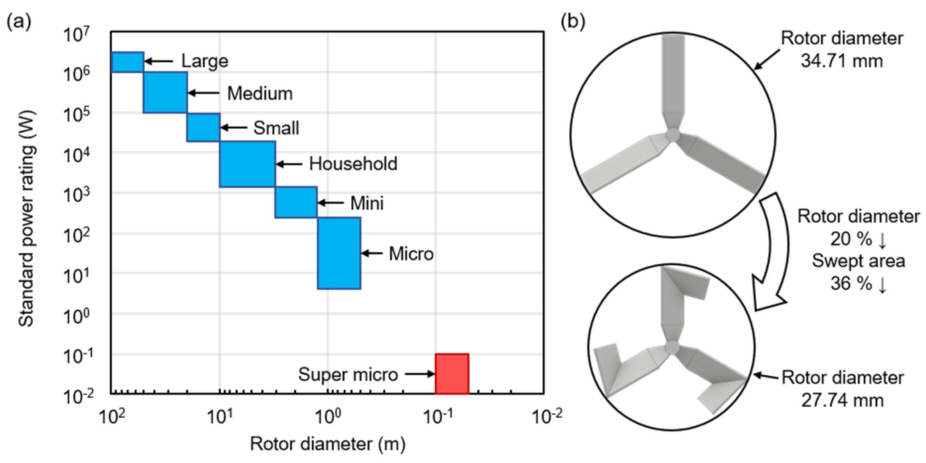
With the increasing resource depletion and global warming, renewable energy sources are being increasingly used as an auxiliary energy source to reduce the use of conventional energy resources based on fossil fuels. Wind energy, as a representative renewable energy source, is used in wind turbines that generate electricity via the wind-induced rotation of the rotor blades. Wind turbines can be classified according to their rotor diameter and generating power (Figure 1a). Large wind turbines, which have a diameter of 50–100 m and generating power of 1–3 MW, generate considerable energy at a relatively low cost; however, the initial cost is extremely high, and such turbines can only be installed in large open onshore or offshore areas. Conversely, small wind turbines with a diameter of less than 10 m and generating power of 20 kW have a considerably low initial cost and can be applied in several regions. Consequently, small wind turbines can generate useful energy even if they are located far from the power grid [1,2].
In this regard, engineers have attempted to use extremely small wind turbines with a diameter of less than 100 mm as an energy harvesting tool for wasted wind energy. An example of such an application is a wireless sensor system operated using a small wind turbine to predict the spread direction of wildfires [3]; specifically, a rotor with a diameter of 60 mm is used to generate electric power for the sensors. In addition, a wind turbine (rotor diameter of 127 mm) was developed to drive a piezoelectric bimorph, which is commonly used in energy harvesting devices, to generate electricity [4,5]. These studies successfully demonstrated that even low-intensity winds can be utilized as an energy source for energy harvesting. However, a considerable scope of improvement remains in terms of space, efficiency, operational scheme, and application strategies of such small turbines.
To improve the conversion efficiency of wind energy to mechanical power, modifying the turbine blades’ shapes is an effective strategy. Hence, it is reasonable to assume that this approach is also valid for extremely small wind turbines. It was noted that for micro wind turbines (with a diameter of 1 m), using a curved blade, mimicking the shape of a bird wing, resulted in an efficiency improvement of 8.1% [6]. Some researchers reported that using a small wind turbine blade having two parts with different pitch angles led to performance enhancement of 16%, compared to that of a model with a constant pitch angle [7]. Thus, modifying the blade geometry is expected to be a valuable strategy in enhancing the performance of extremely small wind turbines for energy harvesting. However, this type of study has not, thus far, been conducted quantitatively.
To this end, a parametric study for the curved blade of an extremely small wind turbine, hereinafter referred to as the “super micro wind turbine” (SMWT), was conducted to quantify the influence of the change in blade geometry on the energy harvesting performance of the turbine, via experimental and three-dimensional (3D) numerical analyses. In this study, a horizontal axis wind turbine was used as it is generally more popular, accessible, and easy to construct and exhibits a higher efficiency than that of a vertical axis turbine [2]. A curved blade design (Figure 1b) was adopted to improve the performance and reduce the rotor diameter of the SMWT. Blades with nine different curved angles were manufactured using a 3D printer, which is often used for fabricating small blades [8], and the output of the SMWT equipped with these blades was measured. The output voltages were measured using an oscilloscope, and the AC was converted to DC using an AC–DC conversion circuit [9]. In addition, to predict the detailed local flows near the curved blade, a 3D standard k-ε turbulence model was applied with steady-state rotation. The pressure distribution and streamlines near the blades were confirmed to evaluate the rotor characteristics according to each angle.
2. Theoretical Background
The governing equations for the flow used in the model during this study are the continuity equation (Equation (1)) and Navier–Stokes equation (Equation (2)) [6,10]. The heat effect is not important in our study, so the energy equation was not used.
The turbulence model selected in this study is a standard k-ε model, which is expressed as follows (Equations (3) and (4)) [10]:
where k is turbulence kinetic energy, ε is dissipation rate, Gk is the generation of turbulence kinetic energy due to the mean velocity gradients (calculated by ), and u’ is turbulence fluctuations. The turbulent (or eddy) viscosity, μt, was calculated as . The constants C1ε, C2ε, Cμ, σk, and σε had the values of 1.44, 1.92, 0.09, 1, and 1.3, respectively. These values have been found to work fairly well for a wide range of wall-bounded and free shear flows [10].
3. Methodology
3.1. Blade Design
In general, the performance of wind turbines often cannot be improved beyond a certain limit by modifying the blade geometry, as the aerodynamic design of the blades must ensure structural safety. Equation (5) shows that a larger blade requires a higher structural stability. Specifically, the axial force acting on the disk (rotor) is proportional to the squared rotor radius [11].
X = ρ·π·r2·c2 (c1 − c3)
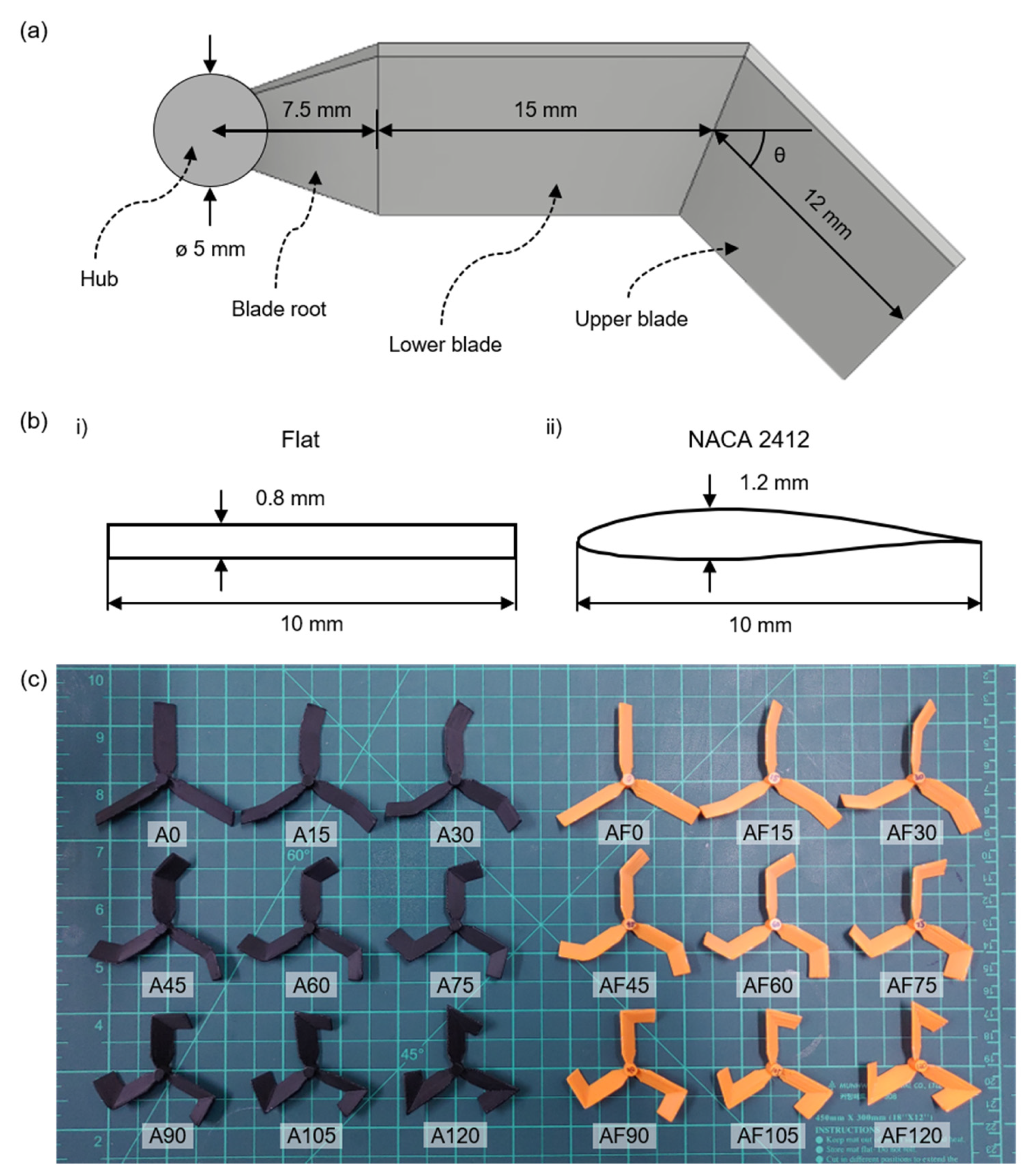
In particular, the rotor used in this work consists of a hub with a diameter of 5 mm and three blades with a length of 34.5 mm. To realize the curved blade, the blade is divided into three parts in the radial direction, namely, blade root, lower blade, and upper blade. The blade root has a length of 7.5 mm in the radial direction from the rotational axis, the lower blade has a length of 15 mm, and the remaining length of 12 mm above the lower blade corresponds to the upper blade. The curved angle θ between the upper and lower blades is a critical design parameter in this study (Figure 2a). The blade profile is that of a flat airfoil with a width, thickness, and angle of attack of 10 mm, 0.8 mm, and 45°, respectively (Figure 2(bi)). Nine models were developed with θ ranging from 0° to 120° in increments of 15°. Each rotor was named as a combination of the letter “A” implying “angle” and the actual θ value (Figure 2c). In addition, to identify any potential effects of the different blade profiles on the results, we compared the abovementioned rotors (with the flat profile) with rotors having the profile of a NACA 2412 airfoil, with the same cross-sectional areas (Figure 2(bii)). The rotors with the NACA 2412 profile are named using the prefix “AF” instead of “A” (Figure 2c).
3.2. Experimental Setup
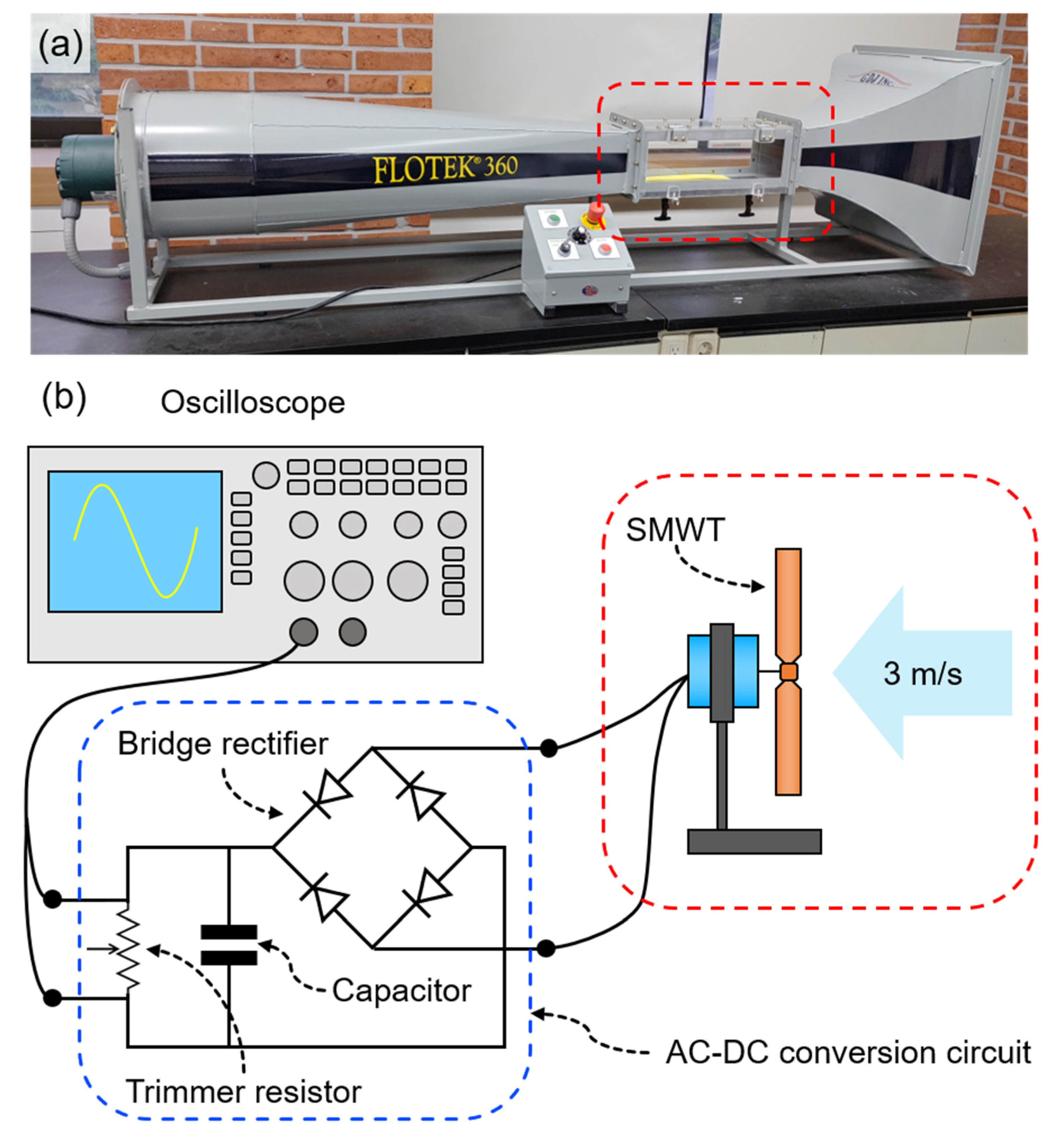
A blade fabricated using 3D printers has been often used in wind turbine experiments [8,12]. In our study, to fabricate the rotors, 3D modeling was performed using Autodesk Inventor 2018 (Autodesk Inc., Mill Valley, CA, USA). The rotors were fabricated using a 3D printer (Style 3DP-210F, Cubicon, Seongnam, Korea). Acrylonitrile butadiene styrene copolymer (ABS, density of 1.04 g/cm3, diameter of 1.75 mm) was used as the printing material. The rotor was fitted to a brushless DC (BLDC) motor (16 × 13.5 × 16 mm, 0.01–15 V, 0.001–0.2 A, AIYIMA, Shenzhen, China). Wind with a speed of 3 m/s was generated using a wind tunnel (Flotek 360, GDJ, Inc., Tyler, OH, USA) and measured using a hot wire anemometer (TES-1341, TES Electrical Electronic Corp., Taiwan). The output voltage was measured using an oscilloscope (TDS2002B, Tektronix, Inc., Beaverton, OR, USA). The average rotational speed was measured using a laser-type tachometer (G8905; Benetech, Shenzhen Jumaoyuan Science and Technology Co., Ltd., Shenzhen, China) to realize the performance evaluation and computational fluid dynamics (CFD) analysis. Figure 3 illustrates the experimental setup. The power consumption cannot be measured at the alternating current (AC) output and was, thus, rectified using a single-phase silicon bridge rectifier (W06M; Dc Components Co, Taiwan). In addition, the voltage was stabilized using a polyester film capacitor (MF 0.1 μF/100 V DC; HyunDai Condenser, Korea). The circuit was configured to adjust the load resistance at 100 kΩ intervals in the range of 100–1000 kΩ using a trimmer resistor (3362P-1-105; Bourns, Inc., Riverside, CA, USA) to identify the change in the electrical power with the load resistance (blue dashed line, Figure 3). This configuration was referred to as the alternating current to direct current (AC–DC) conversion circuit.
3.3. CFD Analysis
CFD analysis has been a popular tool to gain better understanding and visualization in the flow-pressure field around wind turbine blades [13,14]. In this study, a CFD analysis was performed using ANSYS 19.2 Fluent (Ansys, Inc., Canonsburg, PA, USA) to analyze the aerodynamic characteristics of the curved blades. Six representative rotors (i.e., A0, A30, A60, A90, A105, and A120) were analyzed. The flow domain for the analysis was a cylindrical region with a length and diameter of 800 mm and 800 mm, respectively, as shown in Figure 4. The domain diameter was approximately 11 times larger than the rotor diameter to prevent the occurrence of any unwanted boundary effects on the flow near the rotor. The working fluid was air with a density of 1.225 kg/m3 and dynamic viscosity of 1.7894 × 10⁻⁵ kg/m-s. The steady state was assumed, and the k-ε turbulence model was selected to simulate the turbulence. In terms of boundary conditions, a velocity inlet of 3 m/s and pressure outlet of 0 Pa (gauge pressure) were applied. The operating pressure was 101,325 Pa, and the actual rotational speeds measured from the experiments were applied to the CFD analysis.
To realize an accurate simulation, the composition and characterization of the mesh are critical aspects. Herein, a 3D tetrahedral mesh was constructed using Ansys Meshing (Ansys 19.2, Inc., Canonsburg, PA, USA) (Figure 4). Denser meshes were carefully introduced near the blade surface, where complex flow patterns occur, and coarser meshes were used in other areas to increase the computational efficiency (Figure 4b). To verify the reliability of the mesh system, a mesh test was performed for the A0 rotor under three mesh system densities with 671,815 (Grid #1), 1,130,312 (Grid #2), and 2,099,837 (Grid #3) elements. The rotational speed was 1,121 RPM, which was provided in the experiment using the A0 rotor. The surface pressure at a radial distance of 10 mm for the Grid #1 and Grid #3 mesh systems was 5.58% lower and 2.23% higher than that of the Grid #2 mesh system, respectively (Figure S1 in the Supplementary Materials). Therefore, considering the computational efficiency and accuracy, the Grid #2 mesh system was selected.
4. Results and Discussion
4.1. Electrical Power Measurement and Estimation
To fabricate the 3D rotors, including the support, ABS polymer between 1.89 g (for A120, minimum) and 2.12 g (for A15, maximum) was consumed (Figure 2c). The printing time was approximately 30 min per rotor. The mechanical properties of the 3D-printed ABS are about 27% weaker than those of the injection-molded ABS [15,16,17]. However, the rotors fabricated herein operate at low wind speeds (3 m/s), so the difference in mechanical properties due to processing is not significant. In addition, 3D printing has faster processing speed and is more convenient. The target velocity was set to 3.0 m/s in this study. This target velocity value was selected because we focused on an energy harvesting wind turbine system that can react to winds as low as possible and because the small turbine used in this study had a cut-in speed of approximately 2.5 m/s. The rotating speed was measured using a laser-type tachometer (G8905; Benetech, Shenzhen Jumaoyuan Science and Technology Co., Ltd., China).
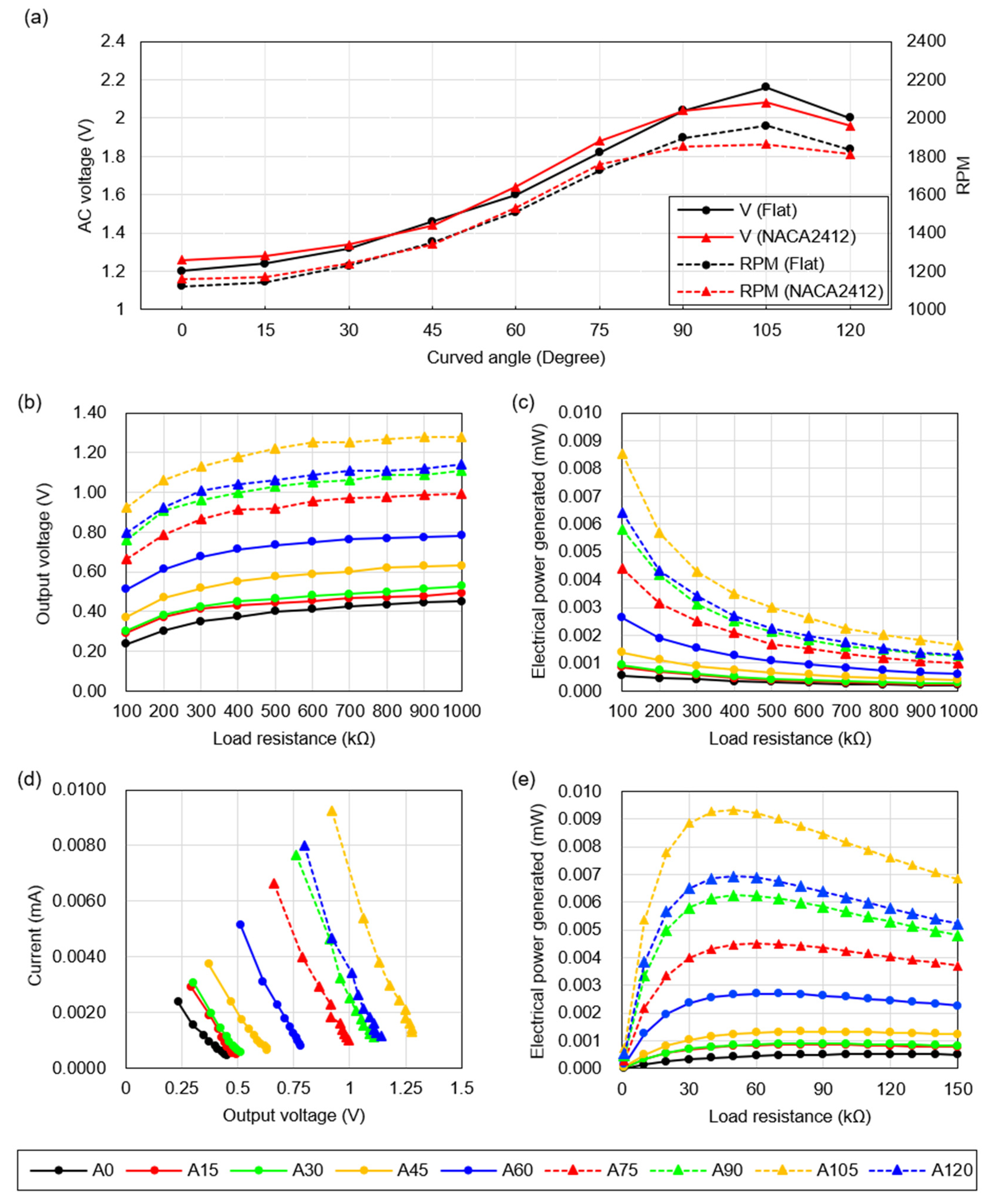
As shown in Figure 5a, for A0, the average rotational speed was 1,120.6 RPM and AC was 1.20 V, which increased to 1,959.4 RPM and 2.16 V for A105, respectively. A particularly rapid increase in the RPM and AC was noted between A30 and A90, in which the blade radius decreased sharply (Table 1). When θ was further increased from 105° to 120°, both the RPM (1,835.7) and AC (2.00 V) for A120 decreased, compared to 1,959.4 RPM and 2.16 V for A105, respectively, as shown in Figure 5a. This result is related to the radius of the rotor (r) and the law of angular momentum conservation. In particular, when the rotor reaches a steady state (i.e., the total rotational force becomes 0), the angular momentum conservation equation, Equation (6), is satisfied [18].
where L is the angular momentum, mi is the element mass of the blades, ri is the rotating radius of a particle, and ω is the angular velocity. According to Equation (6), when ri decreases, ω increases. As shown in Table 1, the radius or the rotor, r, decreases as the curved angle, θ, increases to 105° (A105). However, with further increases in θ to 120° (A120), r increases owing to the geometric interaction of upper and lower blades (Figure S2 of the Supplementary Materials).
ΔL = ∑ mi·ri2·ω
To measure the power, P, the DC voltage must be measured; thus, the AC–DC conversion circuit was used to convert AC to DC. Ohm’s law and the electrical power equation are expressed as in Equations (7) and (8), respectively.
where I is the calculated current, V is the measured output DC voltage, and R is the load resistance. As shown in Figure 5b, the measured DC voltages exhibited the same pattern as that for the AC voltage; a rapid increase was noted from A45 to A105, and the value reduced at A120. The DC voltage increased with the load resistance, R, in the AC–DC conversion circuit, and its slope plateaued at a higher load resistance (Figure 5b). The value of P for each rotor, calculated using Equation (8) exhibited the same pattern as that for the AC, as shown in Figure 5c; a rapid increase occurred from A45 to A105, but the value reduced at A120. With a decrease in R, P increased, and the maximum experimental value occurred at 100 kΩ. To design an actuator operating with the SMWT, the maximum value of power and the load resistance corresponding to this value must be determined. Figure 5c indicates that P is larger at a lower load resistance. Therefore, an estimation model was established to obtain the maximum power, Pmax. The determined I–V curves can be observed to be linear (Figure 5d). Therefore, the estimation model for the linear curve was obtained as given in Equation (9), and Equations (8) and (9) were combined to yield Equation (10).
where Ic, Vc, and Pc denote the calculated current, voltage, and power, respectively; a and b are coefficients that are different for each rotor (Table 2). As mentioned previously, Pmax, depending on the load resistance, must be identified to realize the actuator design. To obtain the Pc–R curve, Vc in Equation (10) should be replaced by the suitable expression for R. The relation for Vc and R is expressed in Equation (11), obtained by combining Equations (7) and (9). Furthermore, by combining Equations (10) and (11), the relation between Pc and R can be established, as expressed in Equation (12).
Ic = a − bVc
Pc = aVc − bVc2
As shown in Figure 5e, Pc exhibited the same pattern as that for the AC voltage: a rapid increase from A45 to A105 and subsequent reduction at A120. In addition, Pc exhibited a local maximum point corresponding to Pmax (μW) for each rotor (Figure 5e). Equation (12) was differentiated to determine the load resistance at the local maximum point to obtain Pmax. The values of Pc and Pmax are listed in Table 2. A105 exhibits the highest Pmax (9.3333 μW) at 47.62 kΩ, which corresponds to the experimental result (Figure 5). As the power of each rotor decreases, the load resistance at Pmax increases, from 47.62 kΩ (A105) to 117.65 kΩ (A0).
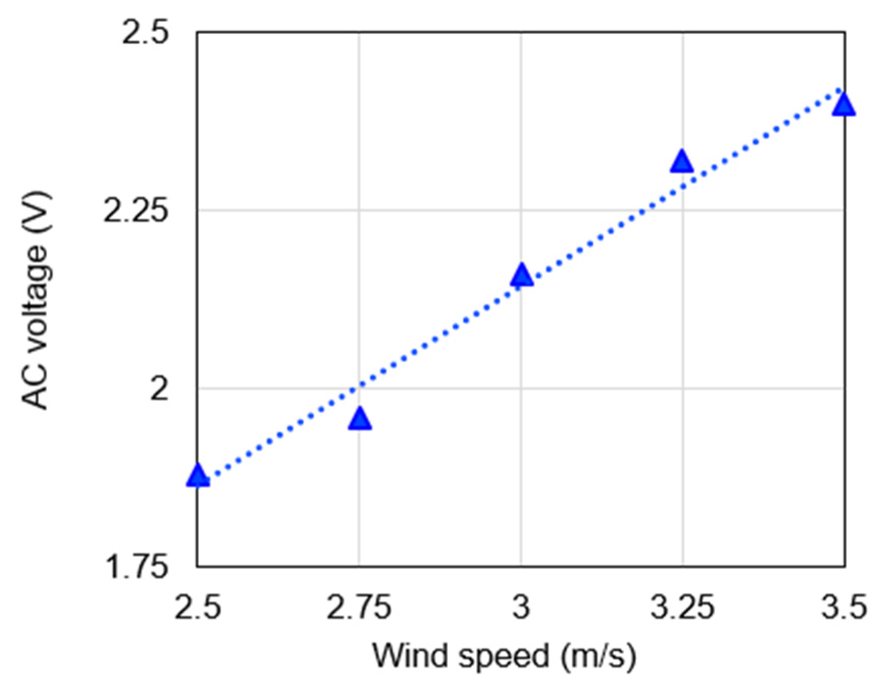
It was set to 3m/s for all experiments and simulations in this paper, however, the wind in real life has a significant amount of variation as the change in wind speed is stochastic. Therefore, it is necessary to investigate the response of our SMWT to these wind speed changes. For this, additional experiments were performed to analyze the change in the output of AC voltage of A105 (as a representative case) according to various wind speeds ranging from 2.5 to 3.5 m/s at 0.25 m/s intervals (Figure 6). The monitored AC voltages were 1.88, 1.96, 2.16, 2.32 and 2.40 V for 2.5, 2.75, 3, 3.25 and 3.5 m/s, respectively, and exhibited a first-order linear relationship (VAC = 0.56u + 0.464 where VAC is the AC voltage and u is the wind speed). This data will be useful in practical energy harvesting applications of our SMWT.
In addition, to inspect the fracture wind speed of the 3D-printed rotor, the A105 rotor, which had the best performance, was tested at high wind speeds (5–27 m/s). The rotor broke at approximately 25 m/s (Video S1), which is the cut-out wind speed of a commercial wind turbine [19,20,21], and the fractured rotor and its cross section are shown in Figure S3 (see the Supplementary Materials).
4.2. CFD Analysis
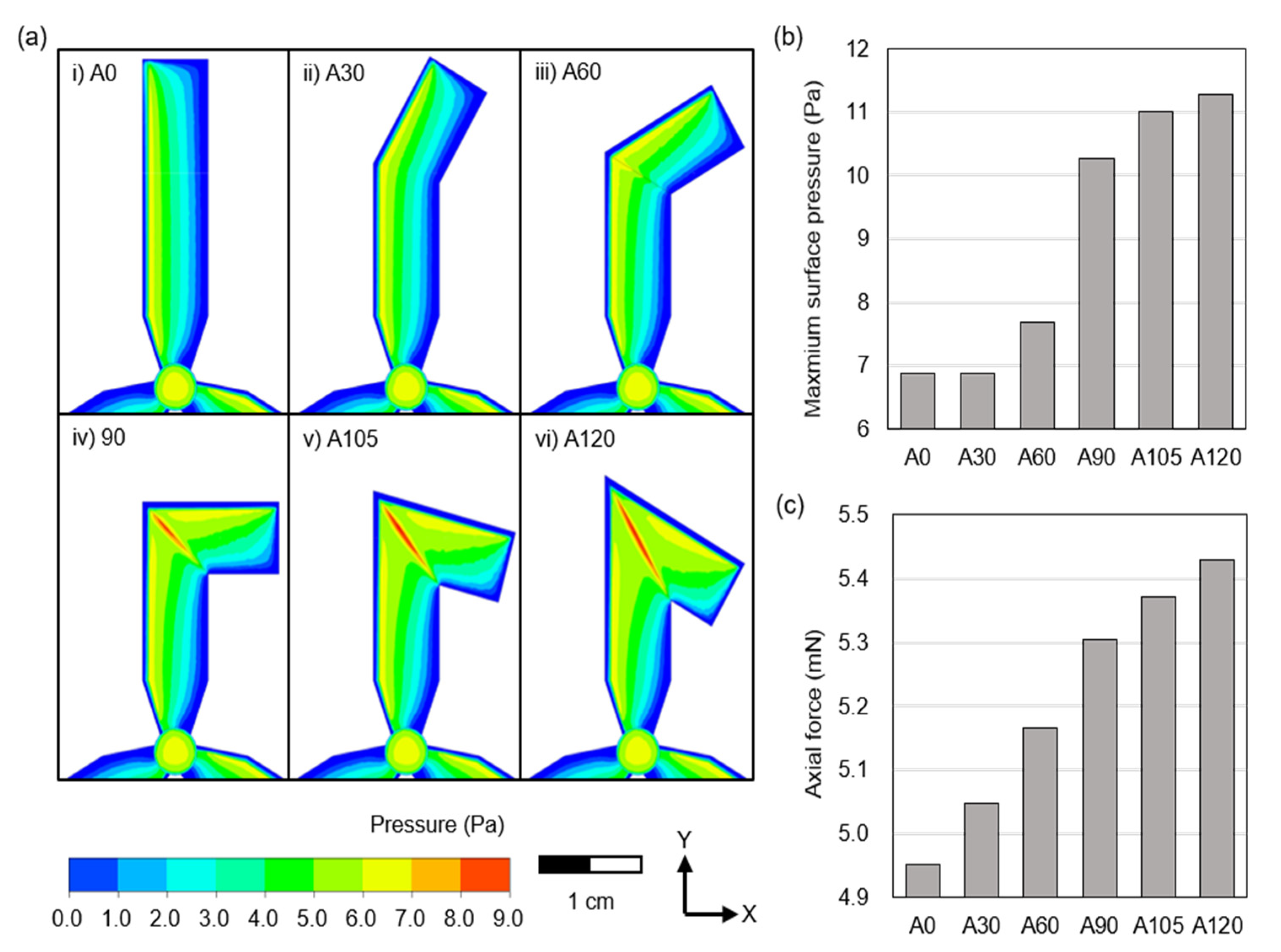
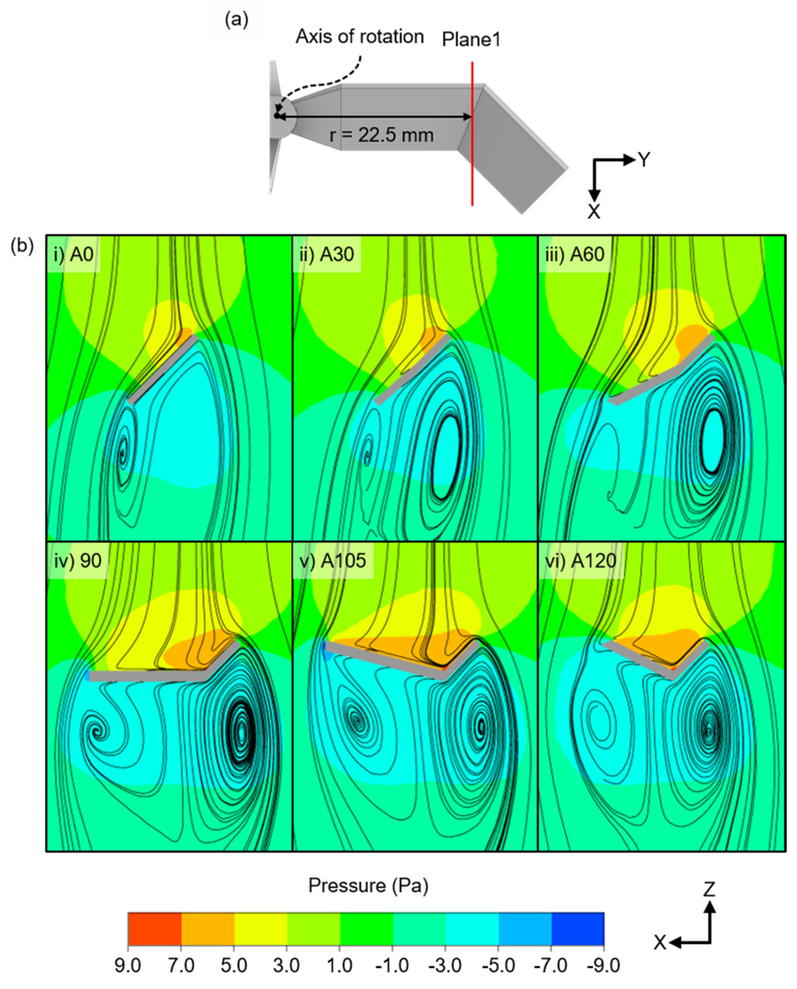
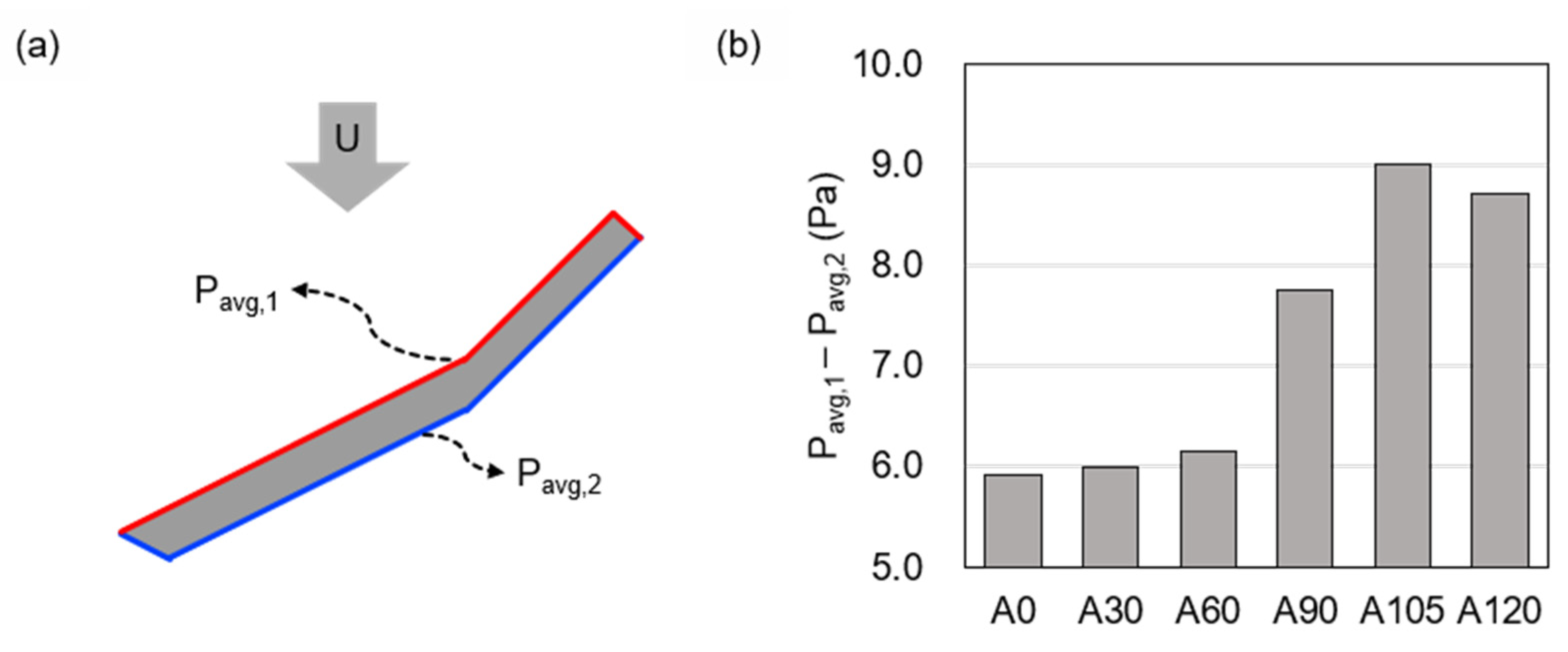
To understand the relationship between θ and the output parameters, a CFD analysis was performed, and the pressure distribution on the blade surface and the streamlines and pressure distribution near the blade were evaluated. A notable characteristic was the increased pressure at the boundary of the upper and lower blades. The pressure contour appeared as a vertical stripe in A0, which is a basic rotor. In A30 and A60, the stripe appeared to be curved along the blade. However, in A90, A105, and A120, the stripe collapsed around the boundary of the upper and lower blades, and the area of the intermediate pressure region (4.0–7.0 Pa) increased. Furthermore, a high-pressure region (7.0–9.0 Pa) was generated along this boundary (Figure 7a). This phenomenon indicates that the force that the wind transmits to the rotor increases with an increase in θ. To clarify the quantitative value of pressure, the maximum surface pressure and axial force acting on the rotor were analyzed. It was noted that the maximum surface pressure gradually increases with θ. However, a large increase occurs between A60 and A90, which is consistent with the experimental result (Figure 7b). In addition, the axial force increases with θ, which indicates that the rotor blades convert the wind to power more efficiently at a large θ (Figure 7c). However, the CFD results (Figure 7) indicated that the value increased between A105 and A120, which is not consistent with the experimental findings, indicating that the value decreased between A105 and A120 (Figure 5). This discrepancy can be understood by confirming the flow around the blade. The streamlines were plotted on plane 1 located 22.5 mm from the axis of rotation, equivalent to the blade curve point (Figure 8a). In the case of A0, which corresponds to the basic rotor whose blades are not curved, a typical form of a streamline and pressure contour passing through an angled plate in the direction of the mainstream is observed (Figure 8(bi)); the wind arrives at the leading edge, creating high pressure, and splits into the right stream moving to the right of the leading edge and the left stream passing outward along the blade surface. In the case of A30 and A60, the high pressure (0.5 < P < 7.0 Pa) region became larger. However, the streamlines were reasonably similar to those of A0 because the angle of the curved section was not sufficiently large to cause a substantial distortion of the streamlines (Figure 8(bii,iii)). In the case of A90, however, a significant difference was noted (Figure 8(biv)) in the streamline, showing that the wind arrived at the trailing edge, which is perpendicular to the mainstream and proceeded to the leading edge instead of moving along the blade surface. Meanwhile, the high pressure (0.5 < P < 7.0 Pa) region extended to the trailing edge, and the pressure difference between the front and rear of the blade was increased. The streamlines and pressure distribution were more prominent in the case of A105 and A120, that is, the blades with a higher θ value (Figure 8(bv,vi)). The streamline and pressure contour near the blade of A90, A105, and A120 implies that the local flow near the blade has a positive effect on improving the rotational speed. Further, the pressure difference between the front and rear of the blade should be investigated since it is closely related to the lift force and, thus, the blade performance. For convenience, the averaged pressure on the front of the blade was called Pavg,1 (red, Figure 9a) and that on the rear of the blade was called Pavg,2 (blue, Figure 9b). The pressure difference of Pavg,1−Pavg,2 increased with θ for A0 ~ A105 and decreased for A120 (Figure 9b), which is similar to the experiment results (Figure 5a–e).
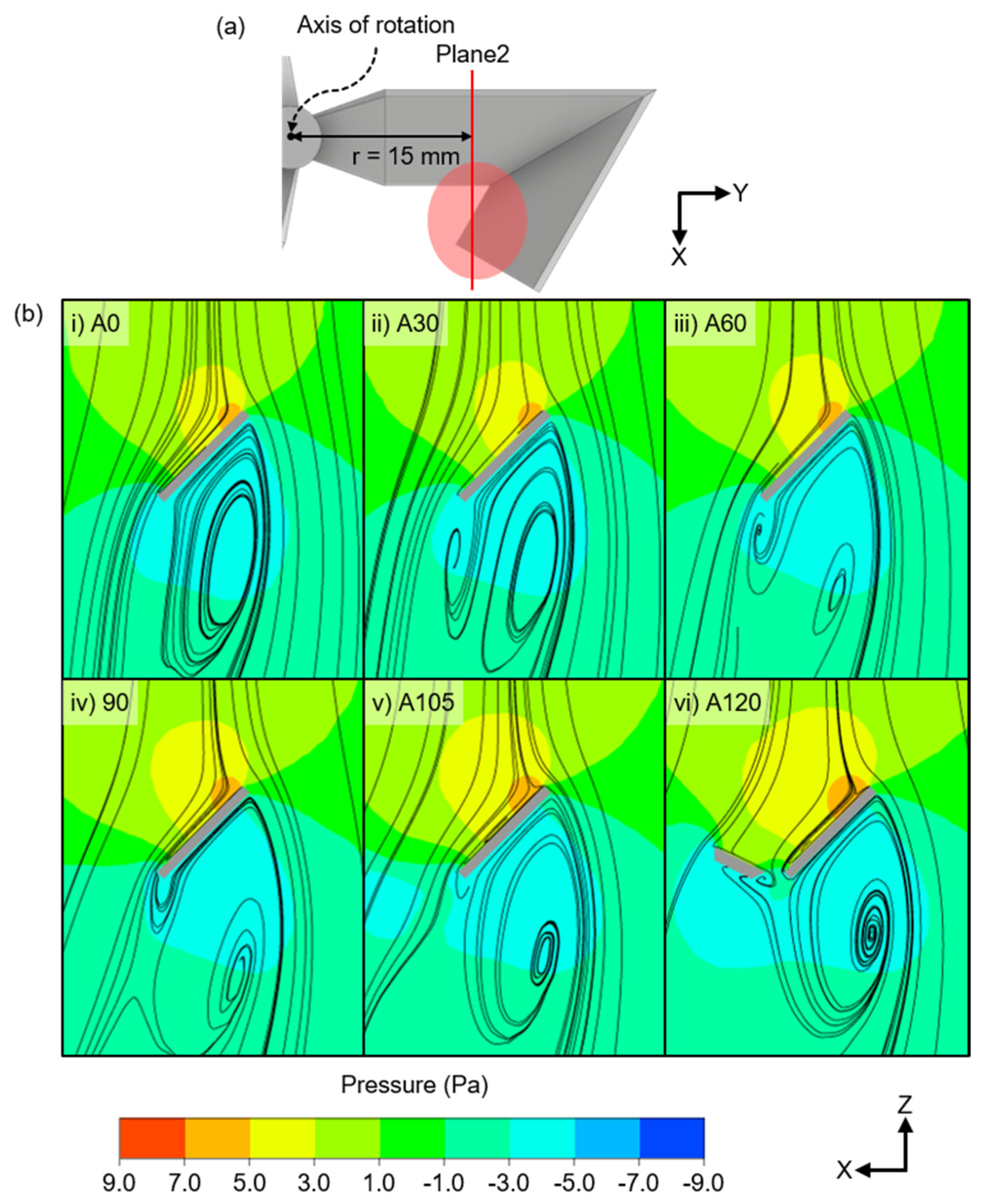
As shown in Figure 10a, at a large θ value, such as in the case of A105 and A120, the tip of the upper blade was located below plane 1. This unique characteristic likely influences the overall streamline pattern. To observe the streamline near this area, the streamlines were plotted on plane 2, located 15 mm from the axis of rotation (Figure 10a). As shown in Figure 10(bi–v), the streamlines and pressure contours for the A0–A105 models exhibit the same characteristics as those for A0 (Figure 8(bi)), except for small differences caused by the upper blade. As shown in Figure 10(bvi), the cross section of the blade was divided into the left and right parts, which were the upper and lower blades, respectively. For both parts, the typical streamline and pressure contour corresponding to a plate being angled to the mainstream were observed. However, because the angle of each blade was different, the forces acted in the opposite directions. In the left part, the force acted in the direction opposite to the rotational direction, thereby disrupting the rotation. Conversely, in the right part, the force acted in the direction of the rotational direction, thereby facilitating the rotation. Such a flow was observed in the cases of A105 and A120. However, in the case of A120, because the upper blade was located further below plane 1, the area was wider, and when the force acting on the left part became sufficiently large to retard rotation, the output AC voltage, DC voltage, and power reduced (Figure 5). Therefore, even if the maximum surface pressure and axial force acting on the rotor are large (Figure 7b,c), performance may deteriorate if the direction in which the force acts is the direction hindering the rotation.
5. Conclusions
Typically, the wind intensity in the urban environment is far too low to be useful for ordinary large-scale wind turbines, and such wind energy is thus often disregarded and wasted. However, from the energy harvesting viewpoint, this wind energy is useful for low-energy consumption applications. The research object in this work was an SMWT, which was used as an energy harvesting system suitable for low wind energy. The electric power generation of the SMWT was characterized in terms of the blade design via both experimental and numerical analyses. Through experiments, the electrical power was confirmed to increase with curved angle and the A105 model (θ = 105°) had the maximum electrical power generation. However, the A120 model (θ = 120°) had lower electrical power generation than the A105 model, which confirms the existence of an optimum curved angle. The experimental result was verified through numerical analysis. In the numerical analysis, it was observed that with an increase in the curved angle of a given blade, the pressure that the wind exerts on the blade increases. The maximum surface pressure and axial force of the A120 model were predicted to be 39% and 9% higher than those for A0, respectively. However, the A120 model exhibited a poorer performance than that of A105 in our experiments. This was also confirmed in the numerical simulation results on the pressure difference between the front and rear blades. This implies that an excessively curved angle could adversely affect the performance, which was also confirmed quantitatively in the numerical analysis by the pressure difference between the front and rear blades, the pressure contours around the blades, and streamlines. At a large curved angle (A105, A120), the upper blade is below the tip of the lower blade, and this area acts in a direction that prevents blade rotation, resulting in the A120 model exhibiting lower electrical power generation than A105. Consequently, the experimental AC voltage improved by 80% and 67% for the A105 and A120 models, respectively, compared to A0. The numerical analysis of the pressure difference between the front and rear blades showed a difference of 52% and 46%, for the A105 and A120 models, respectively, when compared to A0. This study showed how the curved blades for SMWT with proper designs can help not only in directly enhancing the electricity generation performance but also in reducing the rotor diameter and swept area. Although a single SMWT was considered in this work, the proposed concept can be easily expanded for the installation of multiple array SMWTs in a limited space (Figure S4 in the Supplementary Materials), and this can be considered to be a potential candidate as an energy harvesting system to utilize wasted small wind energy to operate various sensors and small Internet of Things (IoTs) that require low power.
Supplementary Materials
The following are available online at https://0-www-mdpi-com.brum.beds.ac.uk/2227-7390/8/8/1295/s1, Figure S1: Result of the grid test. The vertices of the blade cross-section were named counterclockwise ①-④. Cross section of the blades the Grid #1 grid system exhibits a large difference around ① compared to the Grid #2 and Grid #3 grid systems; Figure S2: Rotor radii for the models. The radius of the A0–A90 and A105–A120 rotors is the distance from the hub to the upper and lower blade tips, respectively; Figure S3: Fractured A105 rotor. (a) Rotor fractured at a wind speed around 25 m/s. (b) Fractured cross section of the hub. (c) Fractured cross section of the blade; Figure S4: Multiple array illustration of SMWT. Various arrangements can be applied as desired: (a) grid array, (b) in-line array, and (c) arbitrary array; Video S1: A105 Rotor Hight Wind Intensity Test 0 m/s–27 m/s.
Author Contributions
Conceptualization, J.P. and J.Y.P.; methodology, J.P. and J.Y.P.; software, J.P.; validation, J.P., S.L. and J.Y.P.; formal analysis, J.P.; writing—original draft preparation, J.P. and S.L.; writing—review and editing, J.Y.P.; supervision, J.Y.P.; project administration, J.Y.P.; funding acquisition, J.Y.P. All authors have read and agreed to the published version of the manuscript.
Funding
This research was supported by the Korea Institute of Energy Technology Evaluation and Planning (KETEP) grant (20163010024690) and the Korea Environment Industry & Technology Institute (KEITI) through project for developing innovative drinking water and wastewater technologies, funded by Korea Ministry of Environment (MOE) (2020002690004). This research was also supported by the Chung-Ang University Graduate Research Scholarship in 2019 (J.P.).
Acknowledgments
The authors want to express sincere thanks to Dr. Sung-Hwan Kim from Cell-Smith, Co. for helpful modeling tips.
Conflicts of Interest
The authors declare no conflict of interest.
References
- Clausen, P.D.; Wood, D.H. Research and development issues for small wind turbines. Renew. Energy 1999, 16, 922–927. [Google Scholar] [CrossRef]
- Tummala, A.; Velamati, R.K.; Sinha, D.K.; Indraja, V.; Krishna, V.H. A review on small scale wind turbines. Renew. Sustain. Energy Rev. 2016, 56, 1351–1371. [Google Scholar] [CrossRef]
- Tan, Y.K.; Panda, S.K. Self-autonomous wireless sensor nodes with wind energy harvesting for remote sensing of wind-driven wildfire spread. IEEE Trans. Instrum. Meas. 2011, 60, 1367–1377. [Google Scholar] [CrossRef]
- Myers, R.; Vickers, M.; Kim, H.; Priya, S. Small scale windmill. Appl. Phys. Lett. 2007, 90, 054106. [Google Scholar] [CrossRef]
- Priya, S. Modeling of electric energy harvesting using piezoelectric windmill. Appl. Phys. Lett. 2005, 87, 184101. [Google Scholar] [CrossRef]
- Ikeda, T.; Tanaka, H.; Yoshimura, R.; Noda, R.; Fujii, T.; Liu, H. A robust biomimetic blade design for micro wind turbines. Renew. Energy 2018, 125, 155–165. [Google Scholar] [CrossRef]
- Lanzafame, R.; Messina, M. Design and performance of a double-pitch wind turbine with non-twisted blades. Renew. Energy 2009, 34, 1413–1420. [Google Scholar] [CrossRef]
- Bassett, K.; Carriveau, R.; Ting, D.S.K. 3D printed wind turbines part 1: Design considerations and rapid manufacture potential. Sustain. Energy Technol. Assess. 2015, 11, 186–193. [Google Scholar] [CrossRef]
- Umesh, S.; Venkatesha, L.; Usha, A. Active power factor correction technique for single phase full bridge rectifier. In Proceedings of the 2014 International Conference on Advances in Energy Conversion Technologies—Intelligent Energy Management: Technologies and Challenges, Manipal, India, 23–25 January 2014; pp. 130–135. [Google Scholar]
- ANSYS Inc. ANSYS Fluent, Release 19.1, Help System, Theory Guide; ANSYS Inc.: Canonsburg, PA, USA, 2018. [Google Scholar]
- Dixon, S.; Hall, C. Fluid Mechanics and Thermodynamics of Turbomachinery; Elsevier Ltd.: Oxford, Uk, 2010; ISBN 9781856177931. [Google Scholar]
- Imran, R.M.; Hussain, D.M.A.; Soltani, M. An experimental analysis of the effect of icing on Wind turbine rotor blades. In Proceedings of the IEEE Power Engineering Society Transmission and Distribution Conference, Dallas, TX, USA, 3–5 May 2016; Volume 2016-July. [Google Scholar]
- Elsakka, M.M.; Ingham, D.B.; Ma, L.; Pourkashanian, M. CFD analysis of the angle of attack for a vertical axis wind turbine blade. Energy Convers. Manag. 2019, 182, 154–165. [Google Scholar] [CrossRef]
- Mereu, R.; Passoni, S.; Inzoli, F. Scale-resolving CFD modeling of a thick wind turbine airfoil with application of vortex generators: Validation and sensitivity analyses. Energy 2019, 187, 115969. [Google Scholar] [CrossRef]
- Tymrak, B.M.; Kreiger, M.; Pearce, J.M. Mechanical properties of components fabricated with open-source 3-D printers under realistic environmental conditions. Mater. Des. 2014, 58, 242–246. [Google Scholar] [CrossRef]
- Ozcelik, B.; Ozbay, A.; Demirbas, E. Influence of injection parameters and mold materials on mechanical properties of ABS in plastic injection molding. Int. Commun. Heat Mass Transf. 2010, 37, 1359–1365. [Google Scholar] [CrossRef]
- Wu, W.; Geng, P.; Li, G.; Zhao, D.; Zhang, H.; Zhao, J. Influence of layer thickness and raster angle on the mechanical properties of 3D-printed PEEK and a comparative mechanical study between PEEK and ABS. Materials 2015, 8, 5834–5846. [Google Scholar] [CrossRef] [PubMed]
- Meriam, J.L.; Kraige, L.G.; Bolton, J.N. Engineering Mechanics: Dynamics, 9th ed; John Wiley & Sons: Hoboken, NJ, 2018; ISBN 9781119390985. [Google Scholar]
- Varlas, G.; Steeneveld, G.-J.; Christakos, K.; Cheliotis, I. Offshore wind energy analysis of cyclone Xaver over North Europe. Energy Procedia 2016, 94, 37–44. [Google Scholar]
- Etemaddar, M.; Gao, Z.; Moan, T.; Feng, J.; Zhong Sheng, W. Operating wind turbines in strong wind conditions by using feedforward-feedback control. J. Phys. Conf. Ser. 2014, 555, 12035. [Google Scholar]
- Ishihara, T.; Yamaguchi, A.; Takahara, K.; Mekaru, T.; Matsuura, S. An analysis of damaged wind turbines by Typhoon Maemi in 2003. In Proceedings of the 6th Asia-Pacific Conference on Wind Engineering, Seoul, Korea, 12–14 September 2005. [Google Scholar]
Figure 1.
Wind turbine classification according to the size and scale of the super micro wind turbine (SMWT). (a) Wind turbines are classified considering the size (y-axis) and power generation capacity (x-axis), which are proportional in a logarithmic plot. (b) In super micro wind turbines, the rotating radius can be further reduced by folding the blades.

Figure 2.
Specifications of the curved blade design. (a) The diameter of the hub is 5 mm; the length of the blade root is 7.5 mm; the lengths of the lower and upper blades are 15 and 12 mm, respectively; and the curved angle between the lower and upper blades is θ. (b) Blade profiles of (i) a flat airfoil with a width and thickness of 10 mm and 0.8 mm, respectively, and (ii) a NACA 2412 airfoil with a chord length and thickness of 10 mm and 1.2 mm, respectively. (c) Rotors fabricated using a 3D printer. The black (left) and orange (right) blades employ flat airfoils (10 × 0.8 mm2) and NACA 2412 airfoils, respectively. The background squared paper has grid lines at a 12.7 mm (0.5 in.) interval.

Figure 3.
Experimental setup. (a) Image of the Flotek 360 wind tunnel. The red dashed line is a test section measuring 152 mm × 152 mm × 457 mm. (b) Schematic of voltage measurement. The SMWT is located in the test section, and the wind tunnel generates wind at a velocity of 3 m/s to run the SMWT; the voltage is measured using an oscilloscope. The blue dashed line is the AC–DC conversion circuit that converts AC power to DC power.

Figure 4.
Grid system for computational fluid dynamics (CFD) analysis. (a) The computational domain has a cylindrical shape with a length and diameter of 800 mm and 800 mm, respectively. (b) Grid system around the blade cross-section; denser grids are used near the blade to accurately estimate the pressure and velocity fields.

Figure 5.
SMWT experimental performance graph. (a) AC voltage and rotating speed curves. (b) DC voltage curves for load resistances from 100 to 1,000 kΩ. (c) Power curves for the load resistances from 100 to 1,000 kΩ. (d) I–V curves. (e) Estimated power curves over the load resistance from 0 to 150 kΩ. All the experimental results exhibit an increasing trend from A0 to A105 except in the case of A120.

Figure 6.
AC power and trend line at 2.5–3.5 m/s wind speed on the A105 rotor.

Figure 7.
Pressure contours on the front surface of the SMWT blade. (a) As θ increases, the area of the intermediate pressure region (4.0–7.0 Pa) increases. At θ = 90°, a high-pressure region (7.0–9.0 Pa) occurs along the boundary of the upper and lower blades. (b) Maximum surface pressure on each SMWT rotor. (c) Axial forces acting on each SMWT.

Figure 8.
Calculated streamline and pressure contour at plane 1. (a) Plane 1 is located 22.5 mm from the axis of rotation. (b) Streamline and pressure contour on plane 1. (i) A0, typical form of streamline and pressure contour passing through an angled plate in the direction of flow. (ii) A30, (iii) A60, nearly similar streamlines to that in the case of A0 because of reasonably small θ. The area of the orange region (5.0 < P < 7.0) in front of the leading edge increases with increasing θ. (iv) A90, the wind at the trailing edge proceeded to the leading edge; the wind at the leading edge failed to proceed to the trailing edge and moved to the right of the leading edge. The orange region (5.0 < P < 7.0) constantly expands to the trailing edge. (v) A105, (vi) A120, exhibited more prominent trends than that for A90. The orange area (5.0 < P < 7.0) reaches the trailing edge and fills the front of the blade.

Figure 9.
Pressure difference between the front and rear blades for each blade at plane 1. (a) Schematic of the distinction between the front and rear of the blade. The red and blue lines are the front and back of the blade, respectively, and Pavg,1 and Pavg,2 are the average pressure at that line, respectively. (b) Pressure difference at the front and rear of the blades. The result shows the same pattern as the experiment.

Figure 10.
Location of plane 2 and streamline and pressure contour at this plane. (a) At A120, the tip of the upper blade is located below the tip of the lower blade and plane 2, which is located 15 mm from the rotation axis. (b) Streamline on plane 2. (i) A0, (ii) A30, (iii) A60, (iv) A90, and (v) A105, exhibit a typical form of the streamline passing through an angled plate in the direction of the flow, although small differences occur owing to the upper blade position. (vi) A120, the blade cross-section is divided into left and right parts (upper and lower blade, respectively). The wind pushes the lower blade in the rotational direction; however, the upper blade pushes the wind in the counter-rotational direction, which decreases the rotational speed and deteriorates the performance of the blade.


Table 1.
Rotor radius r for each flat airfoil model.
| Model | Radius, r (mm) |
|---|---|
| A0 | 34.71 |
| A15 | 35.08 |
| A30 | 34.91 |
| A45 | 34.18 |
| A60 | 33.92 |
| A75 | 31.15 |
| A90 | 28.93 |
| A105 | 27.74 |
| A120 | 29.36 |
Table 2.
Coefficient of regression model and calculated output voltage and maximum electronic power.
Table 2.
Coefficient of regression model and calculated output voltage and maximum electronic power.
| Model | a | b | R (kΩ) | Maximum Electrical Power Pmax (μW) |
|---|---|---|---|---|
| A0 | 0.0042 | 0.0085 | 117.65 | 0.5188 |
| A15 | 0.0066 | 0.0126 | 79.37 | 0.8643 |
| A30 | 0.0066 | 0.0120 | 83.33 | 0.9075 |
| A45 | 0.0079 | 0.0117 | 85.47 | 1.3335 |
| A60 | 0.0130 | 0.0156 | 64.10 | 2.7083 |
| A75 | 0.0172 | 0.0164 | 60.98 | 4.5098 |
| A90 | 0.0218 | 0.0190 | 52.63 | 6.2532 |
| A105 | 0.0280 | 0.0210 | 47.62 | 9.3333 |
| A120 | 0.0235 | 0.0199 | 50.25 | 6.9378 |
© 2020 by the authors. Licensee MDPI, Basel, Switzerland. This article is an open access article distributed under the terms and conditions of the Creative Commons Attribution (CC BY) license (http://creativecommons.org/licenses/by/4.0/).
Share and Cite
MDPI and ACS Style
Park, J.; Lee, S.; Park, J.Y. Effects of the Angled Blades of Extremely Small Wind Turbines on Energy Harvesting Performance. Mathematics 2020, 8, 1295. https://0-doi-org.brum.beds.ac.uk/10.3390/math8081295
AMA Style
Park J, Lee S, Park JY. Effects of the Angled Blades of Extremely Small Wind Turbines on Energy Harvesting Performance. Mathematics. 2020; 8(8):1295. https://0-doi-org.brum.beds.ac.uk/10.3390/math8081295
Chicago/Turabian StylePark, Junseon, Seungjin Lee, and Joong Yull Park. 2020. "Effects of the Angled Blades of Extremely Small Wind Turbines on Energy Harvesting Performance" Mathematics 8, no. 8: 1295. https://0-doi-org.brum.beds.ac.uk/10.3390/math8081295
Note that from the first issue of 2016, this journal uses article numbers instead of page numbers. See further details here.