Variational Integrators in Holonomic Mechanics

Abstract

Variational integrators for dynamic systems with holonomic constraints are proposed based on Hamilton’s principle. The variational principle is discretized by approximating the generalized coordinates and Lagrange multipliers by Lagrange polynomials, by approximating the integrals by quadrature rules. Meanwhile, constraint points are defined in order to discrete the holonomic constraints. The functional of the variational principle is divided into two parts, i.e., the action of the unconstrained term and the constrained term and the actions of the unconstrained term and the constrained term are integrated separately using different numerical quadrature rules. The influence of interpolation points, quadrature rule and constraint points on the accuracy of the algorithms is analyzed exhaustively. Properties of the proposed algorithms are investigated using examples. Numerical results show that the proposed algorithms have arbitrary high order, satisfy the holonomic constraints with high precision and provide good performance for long-time integration.

1. Introduction

Numerical integrators for nonlinear dynamic mechanics should reflect the properties of the underlying mechanical systems [1,2]. The characterization of symplectic integrators in terms of variational integrators has proven to be very fruitful. Compared with the traditional algorithms, the variational integrator has clear advantages, such as symplectic preserving, momentum preserving and excellent long-time behaviors [3,4,5].

Variational integrators are based on variational principles. The existence, uniqueness, regularity and other qualitative properties of variational problems have been well studied in appropriate function spaces [6,7]. Based on these studies, variational methods are widely used in mathematics, mechanics, physics, astronomy, economics and other fields of natural sciences and engineering. The theory of the discrete calculus of variations was originally formulated for optimal control problems [8,9,10] and gradually developed into the field of mechanics. Within the scope of discrete mechanics, the discrete Euler–Lagrange equations, the discrete Nother’s theorem and the discrete action sum were clearly understood in [11,12,13], and these theories form the foundation of variational integrators. Using the idea of variational integrators, the Verlet method develops a series of algorithms. The SHAKE algorithm was first proposed by Ryckaert for molecular dynamics in [14] and is a constrained form of the Verlet algorithm. Another constrained version of the velocity Verlet integrator, called RATTLE, was proposed in [15] by Anderson and was later shown to be a symplectic integrator [16]. The Newmark method could be derived from variational integrators by choosing appropriate parameters, and an analysis of the symplecticity was given in [17]. The partitioned Runge–Kutta methods are a class of integrators that generalize the standard Runge–Kutta method. It has also been generalized to multi-symplectic partial differential equations, thus resulting in the multi-symplectic product partitioned Runge–Kutta methods [18]. The spectral and symplectic integrability analysis of the nonlinear dynamical systems are given by Blackmore [19]. Traditionally, variational integrators have been used to study conservative systems [20], but modern variational integrators have been developed for various problems, such as Hamiltonian systems [21,22], Lagrangian PDEs [23,24,25], non-holonomic systems [26,27,28] and forced and controlled systems [29,30,31,32]. By introducing suitable new variables and using integral representations, a dissipative system can be transformed into a system of conservative form; then, the Lagrangian of the associated system can be used to develop a variational integrator that inherits the advantageous properties of the conservative counterpart [33,34].

In recent years, high-order systems have received renewed interest due to new and relevant applications in optimal control for robotics and aeronautics and in the study of air traffic control and computational anatomy [35,36,37]. Galerkin variational integrators comprise a general method for constructing high-order variational integrators. They rely on the discretization of the action, which is then approximated by the finite-dimensional function space and a numerical quadrature rule. For unconstrained systems, the Galerkin variational integrator with the highest order is derived by using the Gauss–Legendre quadrature [5]. When using $m$ degree polynomials for the approximation of the coordinates and the $m$ points Gauss–Legendre quadrature rule, the order of this Galerkin variational integrator is $s=2m$. Meanwhile, for the constrained system, the Galerkin variational integrator with the highest order is constructed by taking the Lobatto quadrature rule [5]. When using $m$ degree polynomials for the approximation of the coordinates and the $m$ points Lobatto quadrature rule, the order of this Galerkin variational integrator is $s=2m-2$.

It is fairly well known that, for a given number of points, the Gauss–Legendre rule has the highest order. However, according to the above discussion, the Gauss–Legendre rule is not used for the constrained system. Recently, a new kind of variational integrator for dynamic systems with holonomic constraints was constructed and analyzed in [38]. In this study, the augmented Lagrangian is split into two parts, which makes it possible to use the Gauss–Legendre quadrature rule for constrained systems. This practice not only improves the accuracy of the algorithm but also makes the construction of the algorithm more flexible. However, the quadrature points for the integral of the constrained term is still restricted to be part of the control points of the Lagrangian multipliers, and this makes it impossible to determine the effect of each factor on the accuracy of the algorithm. Evidently, clarifying the effect of each factor on the accuracy of the algorithm can provide a basis for constructing higher-precision algorithms. In our work, the augmented Lagrangian for constructing variational integrators follows [38]. However, in contrast to [38], the position of quadrature points used by two parts of the integral are both independent of the position of the control points. In this way, we put forward eight algorithms by choosing different types of control points and quadrature points. Based on these eight algorithms, the influence of control points and quadrature points on the accuracy of the algorithm is discussed in detail using numerical examples, and the effect of each factor on the accuracy of the algorithm is determined. This paper is structured as follows. In Section 2, we recall the basic definitions and concepts of constrained variational mechanics and variational integrators. In Section 3, a new construction of the Galerkin variational integrator for the constrained system is presented. In Section 4, the numerical properties are assessed using numerical examples and the influence of control points and quadrature points on the accuracy of the algorithm are discussed. Finally, a conclusion is given in Section 5.

2. Variational Principle for Constrained Mechanics

2.1. Constrained Dynamics

In this section, a brief review of constrained dynamics is presented following [4]. Consider a mechanical system defined on the $d$ dimensional configuration manifold $Q$ with the corresponding tangent bundle $TQ$. Let $q={\left\{q_1,q_2,\cdots ,q_d\right\}}^{\mathrm{T}}\in Q$ and $\dot{q}={\left\{{\dot{q}}_1,{\dot{q}}_2,\cdots ,{\dot{q}}_d\right\}}^{\mathrm{T}}\in T_{q}Q$ be the generalized coordinates and velocity of this system, respectively. Suppose that the system is constrained by $c$ holonomic constraints:

$$g\left(q\right)={\left\{g_1\left(q\right),g_2\left(q\right),\cdots ,g_c\left(q\right)\right\}}^{\mathrm{T}}=0$$

(1)

Then, the dynamic equation of motion for this system is given by

$$\frac{d}{dt}\left(\frac{\partial L}{\partial \dot{q}}\right)-\frac{\partial L}{\partial q}+G^{\mathrm{T}}\left(q\right)\lambda =0$$

(2)

$$g\left(q\right)=0$$

(3)

in which $\lambda ={\left\{{\lambda }_1,{\lambda }_2,\cdots ,{\lambda }_c\right\}}^{\mathrm{T}}$ are the Lagrange multipliers, $G\left(q\right)=\partial g\left(q\right)/\partial q$ is a $c\times d$ matrix, and $L\left(q,\dot{q}\right)$ is the Lagrangian of the unconstrained system.

The action of the constrained system in the time interval $\left[0, T\right]$ is defined as

$$S={\displaystyle {\int }_0^T\left[L\left(q,\dot{q}\right)-g^{\mathrm{T}}\left(q\right)\lambda \right]dt}$$

(4)

and Hamilton’s principle for Equations (2) and (3) can be given by

$$\delta S=\delta {\displaystyle {\int }_0^T\left[L\left(q,\dot{q}\right)-g^{\mathrm{T}}\left(q\right)\lambda \right]dt},\hspace{1em}\delta S=0$$

(5)

If the generalized coordinates at times $t=0$ and $t=T$ are given, such as $\delta q\left(0\right)=\delta q\left(T\right)=0$, then Hamilton’s principle gives Equations (2) and (3).

2.2. Constrained Discrete Variational Dynamics

The concept of variational integrators is based on a discretization of the action. Consider a time grid $\Delta t=\left\{t_k=k\eta |k=0,1,\cdots ,N\right\}$, $N\eta =T$ where $N$ is a positive integer and $\eta$ is the step size. Replace the generalized coordinates $q$ and Lagrange multipliers $\lambda$ by the discrete curve $q_d={\left\{q_k\right\}}_{k=0}^N$ and ${\lambda }_d={\left\{{\lambda }_k\right\}}_{k=0}^N$ with $q_k=q_d\left(t_k\right)$ and ${\lambda }_k={\lambda }_d\left(t_k\right)$ as approximations to $q\left(t_k\right)$ and $\lambda \left(t_k\right)$, respectively. The discrete augmented Lagrangian in interval $\left[t_k, t_{k+1}\right]$ is defined as [38]

$$L_d\left(q_k,q_{k+1},{\lambda }_k,{\lambda }_{k+1}\right)\approx {\displaystyle {\int }_{t_k}^{t_{k+1}}L\left(q,\dot{q}\right)dt}-{\displaystyle {\int }_{t_k}^{t_{k+1}}{g}^{\mathrm{T}}\left(q\right)\lambda dt}$$

(6)

and for the entire time interval $\left[0, T\right]$, the discrete action is defined as

$$S_d\left(q_d,{\lambda }_d\right)={\displaystyle \sum _{k=0}^{N-1}{L}_d\left(q_k,q_{k+1},{\lambda }_k,{\lambda }_{k+1}\right)}$$

(7)

The variation of the discrete action is formulated by finding stationary points of the discrete action given by

$$\delta S_d=0$$

(8)

with $\delta q_0=\delta q_N=0$. Performing the variational calculation gives

$$D_2{L}_d\left(q_{k-1},q_k,{\lambda }_{k-1},{\lambda }_k\right)+D_1{L}_d\left(q_k,q_{k+1},{\lambda }_k,{\lambda }_{k+1}\right)=0,k=1,2,\cdots ,N-1$$

(9)

$$D_3{L}_d\left(q_0,q_1,{\lambda }_0,{\lambda }_1\right)=0$$

(10)

$$D_4{L}_d\left(q_{k-1},q_k,{\lambda }_{k-1},{\lambda }_k\right)+D_3{L}_d\left(q_k,q_{k+1},{\lambda }_k,{\lambda }_{k+1}\right)=0,k=1,2,\cdots ,N-1$$

(11)

$$D_4{L}_d\left(q_{N-1},q_N,{\lambda }_{N-1},{\lambda }_N\right)=0$$

(12)

where $D_i$ denotes the partial derivatives with respect to the i-th variables, respectively, such that

$$D_{i}f\left(x_1,x_2,x_3,x_4\right)=\frac{\partial f\left(x_1,x_2,x_3,x_4\right)}{\partial x_i},\hspace{1em}i=1,2,\dots ,4$$

(13)

Equations (9) and (11) provide a discrete iteration scheme for Equations (2) and (3) that determines $q_{k+1}$ and ${\lambda }_{k+1}$ for given $q_{k-1}$, $q_k$, ${\lambda }_{k-1}$ and ${\lambda }_k$.

3. Galerkin Variational Integrators for Holonomic Constrained Systems

3.1. Galerkin Methods

To obtain accurate variational integrators, the discrete action should approximate the action over short intervals. One way to do this is to approximate the generalized coordinates and Lagrange multipliers via polynomials and approximate the integral via numerical quadrature rules. This approximation can be shown to be equivalent both to a class of continuous Galerkin methods and to a subset of symplectic partitioned Runge–Kutta methods [4].

The construction of our new algorithms falls within the framework of generalized Galerkin variational integrators, which were studied and analyzed in [4,38,39,40,41]. In this section, we first provide a brief review of the generalized Galerkin variational integrators and two well-known algorithms in unconstrained systems. Then, they are generalized to the holonomic constrained systems. By comparing the order of the algorithms in the unconstrained and constrained systems, some contradictions inspire us to develop new algorithms for constrained systems.

For unconstrained systems, the exact discrete Lagrangian $L_d^E$ of the first time interval $\left[0,\eta \right]$ is

$$L_d^E\left(q_0,q_1,\eta \right)={\displaystyle {\int }_0^{\eta }L\left(q,\dot{q}\right)dt}$$

(14)

The motivating idea of the generalized Galerkin variational integrators is to replace the generally non-computable exact discrete Lagrangian $L_d^E\left(q_0,q_1\right)$ with a highly accurate computable discrete analogue $L_d\left(q_0,q_1\right)$. Specifically, given a Lagrangian $L$ and $t\in \left[0, \eta \right]$, the construction of a Galerkin variational integrator for unconstrained systems can be divided into two factors [39]:

• Control points: Choose $n+1$ control points $0=d_0<d_1<\cdots <d_{n-1}<d_n=1$ that determine an $n$ order polynomial space to approximate the space of trajectories
• Quadrature rule: Choose a $g$ point quadrature rule $\zeta (.)$ that satisfies $\zeta \left(f\right)=\eta {\displaystyle \sum _{i=1}^g{b}_{i}f\left(c_i\eta \right)}\approx {\displaystyle {\int }_0^{\eta }f\left(t\right)dt}$ in the time interval $\left[0, 1\right]$ with integral points $0\le c_1<c_2<\cdots <c_{g-1}<c_g\le 1$ and weight $b_i$, $i=1,2,\cdots ,g$ to approximate the integral of the Lagrangian.

In [5,39], the Galerkin variational integrators are based on the $m$ points Gauss–Legendre quadrature rules, and choosing $m+1$ equidistant points as the control points is shown to be equivalent to the collocation Gauss–Legendre method of order $s=2m$. If the system is stiff, better numerical performance will result from using the $m$ points Lobatto quadrature rule and $m+1$ Lobatto points as the control points. The Galerkin variational integrator generated in this way has the order of $s=2m-2$.

The collocation of the Gauss–Legendre method and the Lobatto IIIA–IIIB partitioned Runge–Kutta method provides the best two methods for the unconstrained system. Now, we extend them into the holonomic constrained systems. Due to the existence of constraints given by Equation (1), the construction of a Galerkin variational integrator in constrained systems includes one more factor than in unconstrained systems, i.e.,

• Constraint points: Choose $r+1$ constraint points $0=a_0<a_1<\cdots <a_{r-1}<a_r=1$ so that Equation (1) can be accurately satisfied at time $a_i\eta$, such that $g\left(q\left(a_i\eta \right)\right)=0$ for $i=0,1,\cdots ,r$.

For constrained systems, Galerkin variational integrators based on the $m$ points Lobatto quadrature rule with the choice of the $m$ Lobatto points as the control points and constraint points is shown to be equivalent to the constrained Lobatto IIIA–IIIB partitioned Runge–Kutta method of order $s=2m-2$ [5,38], which is most widely used for constrained systems. However, at first glance, it seems natural to consider a Galerkin variational integrator based on the Gauss–Legendre quadrature rule, which has the highest order for a given number of quadrature points. Thus, we implemented this algorithm by using the $m$ points Gauss–Legendre quadrature rule and equidistant points as the control points and constraint points. The order of the resulting algorithm is listed in

Table 1. Numerical convergence order of the algorithm using the $m$ points Gauss–Legendre quadrature rule and $m$ equidistant control points in constrained system.

$m$	2	3	4	5	6	7	8	9
$s$	2	4	4	6	6	8	8	10

, which shows that the order does not grow linearly as $m$ increases, and it is far below $s=2m-2$.

It is well known that, for a given number of quadrature points $m$, the order of the Gauss–Legendre quadrature rule and the Lobatto quadrature rule are $2m$ and $2m-2$, respectively. Based on the above discussion, it is clear that, in unconstrained systems, the order of the quadrature rules are completely preserved by the collocation of the Gauss–Legendre method and the Lobatto IIIA–IIIB partitioned Runge–Kutta method. However, in constrained systems, the algorithm with the Gauss–Legendre quadrature rule, which should have the highest order, does not achieve the order of $2m$, and this inspires us to explore better algorithms for constrained systems.

3.2. New Construction of Galerkin Variational Integrators for Constrained Systems

Considering the first time interval $\left[0, \eta \right]$, the generalized coordinates $q_i\left(t\right)$ and the Lagrange multipliers ${\lambda }_i\left(t\right)$ are approximated by the Lagrange polynomials of degree $n$ that interpolate $n+1$ control points at time $d_k\eta$, $\left(0=d_0<d_1<\cdots <d_{n-1}<d_n=1\right)$, i.e.,

$$q_i\left(t\right)={\displaystyle \sum _{k=0}^n{N}_k\left(t\right)q_{0,i}^k},\hspace{1em}i=1,2,\cdots ,d$$

(15)

$${\lambda }_i\left(t\right)={\displaystyle \sum _{k=0}^n{N}_k\left(t\right){\lambda }_{0,i}^k},\hspace{1em}i=1,2,\cdots ,c$$

(16)

in which

$$q_{0,i}^k=q_i\left(d_k\eta \right), i=1,2,\cdots ,d, k=0,1,\cdots ,n$$

(17)

$${\lambda }_{0,i}^k={\lambda }_i\left(d_k\eta \right), i=1,2,\cdots ,c, k=0,1,\cdots ,n$$

(18)

$$N_k\left(\tau \right)={\displaystyle \prod _{i=0,i\ne k}^n\frac{\tau -d_i\eta }{d_k\eta -d_i\eta }}, k=0,1,\cdots ,n$$

(19)

Then, the generalized coordinate and Lagrange multiplier vectors can be written as

$$q\left(t\right)={\displaystyle \sum _{k=0}^n{N}_k\left(t\right)q_0^k}, \lambda \left(t\right)={\displaystyle \sum _{k=0}^n{N}_k\left(t\right){\lambda }_0^k}$$

(20)

in which

$$q_0^k={\left\{q_{0,1}^k,q_{0,2}^k,\cdots ,q_{0,d}^k\right\}}^{\mathrm{T}}, {\lambda }_0^k={\left\{{\lambda }_{0,1}^k,{\lambda }_{0,2}^k,\cdots ,{\lambda }_{0,c}^k\right\}}^{\mathrm{T}}, k=0,1,\cdots ,n$$

(21)

Substituting the approximate generalized coordinates and Lagrange multipliers into Equation (4) gives

$$\begin{array}{l}{S}_d\left(q_0^0,q_0^1,\cdots ,q_0^n;{\lambda }_0^0,{\lambda }_0^1,\cdots ,{\lambda }_0^n\right)\\ ={\overline{L}}_d\left(q_0^0,q_0^1,\cdots ,q_0^n\right)-{\overline{g}}_d\left(q_0^0,q_0^1,\cdots ,q_0^n;{\lambda }_0^0,{\lambda }_0^1,\cdots ,{\lambda }_0^n\right)\end{array}$$

(22)

in which

$$\begin{array}{l}{\overline{L}}_d\left(q_0^0,q_0^1,\cdots ,q_0^n\right)={\displaystyle {\int }_0^{\eta }L\left({\displaystyle \sum _{k=0}^n{N}_k\left(t\right)q_0^k};{\displaystyle \sum _{k=0}^n{\dot{N}}_k\left(t\right)q_0^k}\right)}dt\\ {\overline{g}}_d\left(q_0^0,q_0^1,\cdots ,q_0^n;{\lambda }_0^0,{\lambda }_0^1,\cdots ,{\lambda }_0^n\right)={\displaystyle {\int }_0^{\eta }{g}^{\mathrm{T}}\left({\displaystyle \sum _{k=0}^n{N}_k\left(t\right)q_0^k}\right){\displaystyle \sum _{k=0}^n{N}_k\left(t\right){\lambda }_0^k}dt}\end{array}$$

(23)

where ${\overline{L}}_d$ and ${\overline{g}}_d$ denote the approximate actions of the unconstrained term and the constrained term, respectively.

Since $S_d$ depends on variables $q_0^0,q_0^1,\cdots ,q_0^n$ and ${\lambda }_0^0,{\lambda }_0^1,\cdots ,{\lambda }_0^n$, the total differential of $S_d$ is given by

$$\begin{array}{cc}d{S}_d& =\frac{\partial S_d}{\partial q_0^0}d{q}_0^0+\frac{\partial S_d}{\partial q_0^1}d{q}_0^1+\cdots +\frac{\partial S_d}{\partial q_0^{n-1}}d{q}_0^{n-1}+\frac{\partial S_d}{\partial q_0^n}d{q}_0^n\hfill \\ & +\frac{\partial S_d}{\partial {\lambda }_0^0}d{\lambda }_0^0+\frac{\partial S_d}{\partial {\lambda }_0^1}d{\lambda }_0^1+\cdots +\frac{\partial S_d}{\partial {\lambda }_0^{n-1}}d{\lambda }_0^{n-1}+\frac{\partial S_d}{\partial {\lambda }_0^n}d{\lambda }_0^n\hfill \end{array}$$

(24)

Taking $q_0^0$ and $q_0^n$ as the independent variables, and using the theory of generating functions [5], the action $S_d$ satisfies the following equation:

$$d{S}_d=-p_0^{0}d{q}_0^0+p_0^{n}d{q}_0^n$$

(25)

Comparing Equations (24) and (25), the partial derivative of $S_d$ with respect to $q_0^0,q_0^1,\cdots ,q_0^n$, gives

$$\begin{array}{l}-p_0^0=\frac{\partial {\overline{S}}_d}{\partial q_0^0}-\frac{\partial {\overline{g}}_d}{\partial q_0^0}\\ 0=\frac{\partial {\overline{S}}_d}{\partial q_0^i}-\frac{\partial {\overline{g}}_d}{\partial q_0^i},i=1,2,\cdots ,n-1\\ p_0^n=\frac{\partial {\overline{S}}_d}{\partial q_0^n}-\frac{\partial {\overline{g}}_d}{\partial q_0^n}\end{array}$$

(26)

and the partial derivative of $S_d$ with respect to ${\lambda }_0^0,{\lambda }_0^1,\cdots ,{\lambda }_0^n$, gives

$$0=\frac{\partial {\overline{g}}_d}{\partial {\lambda }_0^i},i=0,1,\cdots ,n$$

(27)

As mentioned in Section 3.1, the integrals of action $S_d$ will be approximated by numerical integrations. With integral points $0\le c_1<c_2<\cdots <c_{g-1}<c_g\le 1$ and weight $b_i$, $i=1,2,\cdots ,g$, Equation (27) gives

$$\begin{array}{cc}\frac{\partial {\overline{g}}_d}{\partial {\lambda }_0^i}& ={\displaystyle {\int }_0^{\eta }{g}^{\mathrm{T}}\left({\displaystyle \sum _{k=0}^n{N}_k\left(t\right)q_0^k}\right)N_i\left(t\right)dt}\hfill \\ & ={\displaystyle \sum _{j=1}^g{b}_j{g}^{\mathrm{T}}\left({\displaystyle \sum _{k=0}^n{N}_k\left(c_j\eta \right)q_0^k}\right)N_i\left(c_j\eta \right)},i=0,1,\cdots ,n\hfill \end{array}$$

(28)

in which $N_i$ is the Lagrange polynomial obtained by Equation (19). When the position of the interpolation points of the Lagrange polynomials coincides with the position of the integral points $c_i$, the Lagrange polynomial $N_i$ satisfies $N_i\left(c_j\eta \right)=0$ for $j\ne i$ and $N_i\left(c_j\eta \right)=1$ for $j=i$. Then, Equation (28) gives

$$\frac{\partial {\overline{g}}_d}{\partial {\lambda }_0^i}=g\left(q_0^i\right),i=1,2,\cdots ,n$$

(29)

In this condition, Equation (29) can be written as the following equation:

$$D={\left\{g^{\mathrm{T}}\left(q_0^1\right),g^{\mathrm{T}}\left(q_0^2\right),\cdots ,g^{\mathrm{T}}\left(q_0^n\right)\right\}}^{\mathrm{T}}=0$$

(30)

When the position of the interpolation points of the Lagrange polynomials does not coincide with the position of the integral points, Equation (30) is still used to replace Equation (29) as it can ensure that the holonomic constraints precisely satisfied on the interpolation points. Moreover, Equation (27) includes $\left(n+1\right)c$ equations while Equation (30) includes $nc$ equations, so that $c$ additional equations are required for replacing Equation (27). Here, the velocity constraint at time $t=\eta$ is used, i.e.,

$$V=G\left(q_0^n\right)\frac{\partial H}{\partial p}\left(q_0^n,p_0^n\right)=0$$

(31)

Therefore, Equation (27) is replaced by Equations (30) and (31), in which Equation (30) precisely satisfies the holonomic constraints at control points and Equation (31) satisfies the velocity constraint at the terminal time of the subintervals. So far, the problem of solving holonomic constrained systems is transformed into solving Equations (26), (30) and (31).

Let

$$\overline{q}=\left\{{\left(q_0^1\right)}^{\mathrm{T}},{\left(q_0^2\right)}^{\mathrm{T}},\cdots ,{\left(q_0^n\right)}^{\mathrm{T}}\right\},\widehat{\lambda }=\left\{{\left({\lambda }_0^0\right)}^{\mathrm{T}},{\left({\lambda }_0^1\right)}^{\mathrm{T}},\cdots ,{\left({\lambda }_0^n\right)}^{\mathrm{T}}\right\}$$

(32)

$$N=\left\{N_0,N_1,\cdots ,N_n\right\},\overline{N}=\left\{N_1,N_2,\cdots ,N_n\right\}$$

(33)

and define the Kronecker product of matrix $A\in R^{k\times l}$ and $B\in R^{s\times t}$ as the matrix $A\otimes B\in R^{ks\times lt}$

$$A\otimes B=\left[\begin{array}{ccc}{a}_{11}B& \cdots & a_{1l}B\\ ⋮& \ddots & ⋮\\ a_{k1}B& \cdots & a_{kl}B\end{array}\right]$$

(34)

Then, Equation (26) can be written as

$$E\left(\overline{q},\widehat{\lambda },p_0^n\right)={\displaystyle {\int }_0^{\eta }\left(N^{\mathrm{T}}\otimes \frac{\partial L}{\partial q}+{\dot{N}}^{\mathrm{T}}\otimes \frac{\partial L}{\partial \dot{q}}\right)}dt-{\displaystyle {\int }_0^{\eta }{N}^{\mathrm{T}}\otimes \left[G^{\mathrm{T}}\left(q\right)\lambda \right]dt}+\left\{\begin{array}{c}{p}_0^0\\ 0\\ ⋮\\ 0\\ -p_0^n\end{array}\right\}=0$$

(35)

The variables $q_0^0$ and $p_0^0$ are known; thus, Equations (30), (31) and (35) include $\left(n+1\right)\left(d+c\right)$ equations that are dependent on $\left(n+1\right)\left(d+c\right)$ variables $\overline{q}$, $p_0^n$ and $\widehat{\lambda }$. In this paper, the Newton iteration method is used to solve these nonlinear algebraic equations. The Jacobi matrix $\Psi$ of Equation (30), (31) and (35) with respect to variables $\overline{q}$, $p_0^n$ and $\widehat{\lambda }$ can be given as a block matrix

$$\Psi =\left[\begin{array}{ccc}{\Psi }_{11}& {\Psi }_{12}& {\Psi }_{13}\\ {\Psi }_{21}& {\Psi }_{22}& {\Psi }_{23}\\ {\Psi }_{31}& {\Psi }_{32}& {\Psi }_{33}\end{array}\right]$$

(36)

in which

$$\begin{array}{cc}{\Psi }_{11}& =\frac{\partial E}{\partial \overline{q}}\hfill \\ & ={\displaystyle {\int }_0^{\eta }\left\{\left(N^{\mathrm{T}}\overline{N}\right)\otimes \frac{{\partial }^{2}L}{\partial q\partial q}+\left(N^{\mathrm{T}}\dot{\overline{N}}\right)\otimes \frac{{\partial }^{2}L}{\partial q\partial \dot{q}}+\left({\dot{N}}^{\mathrm{T}}\overline{N}\right)\otimes \frac{{\partial }^{2}L}{\partial \dot{q}\partial q}+\left({\dot{N}}^{\mathrm{T}}\dot{\overline{N}}\right)\otimes \frac{{\partial }^{2}L}{\partial \dot{q}\partial \dot{q}}\right\}}dt-\hfill \\ & {\displaystyle {\int }_0^{\eta }\left(N^{\mathrm{T}}\overline{N}\right)\otimes \frac{\partial G^{\mathrm{T}}}{\partial q}\left(q\right)\lambda dt}\hfill \end{array}$$

(37)

$${\Psi }_{12}=\frac{\partial E}{\partial \widehat{\lambda }}=-{\displaystyle {\int }_0^{\eta }{N}^{\mathrm{T}}N\otimes G^{\mathrm{T}}\left(q\right)dt}$$

(38)

$${\Psi }_{13}=\frac{\partial E}{\partial p_0^n}=\left[\begin{array}{c}0\\ ⋮\\ 0\\ -I_d\end{array}\right]$$

(39)

$${\Psi }_{21}=\frac{\partial D}{\partial \overline{q}}=\mathrm{diag}\left(\left[\begin{array}{cccc}G\left(q_0^1\right)& G\left(q_0^2\right)& \cdots & G\left(q_0^n\right)\end{array}\right]\right)$$

(40)

$${\Psi }_{22}=\frac{\partial D}{\partial \widehat{\lambda }}=0$$

(41)

$${\Psi }_{23}=\frac{\partial D}{\partial p_0^n}=0$$

(42)

$${\Psi }_{31}=\frac{\partial V}{\partial \overline{q}}=\left[\begin{array}{cccc}0& \cdots & 0& \frac{\partial G}{\partial q}\left(q_0^n\right)\frac{\partial H}{\partial p}\left(q_0^n,p_0^n\right)+G\left(q_0^n\right)\frac{{\partial }^{2}H}{\partial p\partial q}\left(q_0^n,p_0^n\right)\end{array}\right]$$

(43)

$${\Psi }_{32}=\frac{\partial V}{\partial \widehat{\lambda }}=0$$

(44)

$${\Psi }_{33}=\frac{\partial V}{\partial p_0^n}=G\left(q_0^n\right)\frac{{\partial }^{2}H}{\partial p\partial p}\left(q_0^n,p_0^n\right)$$

(45)

As mentioned in Section 3.1, the construction of a Galerkin variational integrator in a constrained system depends on three factors: control points, quadrature rules and constraint points. Combined with the construction process given in this section, it is clear that in Equations (30), (31) and (35), the approximation of the generalized coordinates and the Lagrange multipliers depends on the control points, the approximation of the integral depends on the quadrature rules, and the approximation of the holonomic constraint depends on the constraint points. Furthermore, from Equation (30), we can see that the position of the constraint point is actually determined by the control points. Therefore, different algorithms can be constructed by choosing different control points and quadrature rules.

In Section 3.1, we have discussed four Galerkin variational integrators: two for the unconstrained system and two for the constrained system. This shows that the variational integrators for the constrained system do not achieve the expected order. In our research, the variational integrator does not prevent the position of quadrature points from being the same as the position of the control points. This practice not only makes the construction more flexible and general but also makes it possible to determine the effect of quadrature points and control points on the accuracy of the algorithm. Evidently, clarifying the effect of each factor on the accuracy of the algorithm can provide a basis for constructing higher-precision algorithms. To do this, several new Galerkin variational integrators are implemented following the proposed procedure. Two kinds of control points are studied (equidistant control points and Lobatto control points), and two kinds of quadrature rules are studied (Gauss–Legendre quadrature and Lobatto quadrature). Furthermore, the approximate action in Equation (22) is divided into two parts that can be integrated independently. Therefore, we choose different quadrature rules for them to give insight into the quadrature rule. Then, eight algorithms can be constructed by choosing different control points and quadrature rules. The algorithms and their corresponding control points and quadrature rules are listed in

Table 2. Eight algorithms and their corresponding control points and quadrature rules.

	Control Point	Quadrature Rule for Unconstrained Item	Quadrature Rule for Constrained Item
ELL	Equidistant point	Lobatto quadrature rule	Lobatto quadrature rule
EGL	Equidistant point	Gauss–Legendre quadrature rule	Lobatto quadrature rule
ELG	Equidistant point	Lobatto quadrature rule	Gauss–Legendre quadrature rule
EGG	Equidistant point	Gauss–Legendre quadrature rule	Gauss–Legendre quadrature rule
LLL	Lobatto point	Lobatto quadrature rule	Lobatto quadrature rule
LGL	Lobatto point	Gauss–Legendre quadrature rule	Lobatto quadrature rule
LLG	Lobatto point	Lobatto quadrature rule	Gauss–Legendre quadrature rule
LGG	Lobatto point	Gauss–Legendre quadrature rule	Gauss–Legendre quadrature rule

. Based on the comparison and analysis of these algorithms, the influence factors are explored, providing the general notion for building a better algorithm for constrained systems.

4. Numerical Examples and Discussion

4.1. Common Features of the Examples

In this paper, we use dimensionless quantities and the quadruple precision floating-point format for all numerical examples. Since the Hamiltonian is a first integral, the relative error $e_H$ of the Hamiltonian can be defined as

$$e_H=\frac{H_k-H_0}{H_0}$$

(46)

in which $H_k$ is the Hamiltonian at time $k\eta$, and $H_0$ is the exact value of the Hamiltonian. The global error $e$ can be given by

$$e=\max \left(\left|e_H\right|\right)$$

(47)

If the order of an algorithm is $s$, the numerical error for time step $\eta$ is $C{\eta }^s$, in which $C$ is a constant. Thus, the errors $e_1$ and $e_2$ for two different time steps ${\eta }_1$ and ${\eta }_2$ can be given by

$$e_1=C{\eta }_1^s,e_2=C{\eta }_2^s$$

(48)

and the order of the algorithm can be given by

$$s=\left[\log \left(e_1\right)-\log \left(e_2\right)\right]/\left[\log \left({\eta }_1\right)-\log \left({\eta }_2\right)\right].$$

(49)

4.2. Example 1: The Nonlinear Spring Pendulum

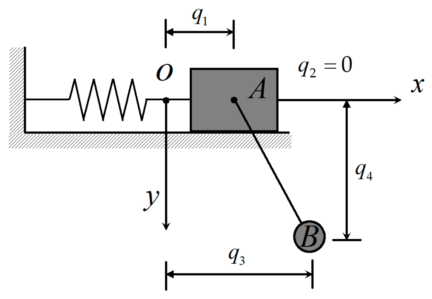
Consider a dynamic system that consists of a nonlinear spring, a point particle $A$ with mass $m_1$, generalized coordinates $\left(q_1,q_2\right)$ and a pendulum $B$ with mass $m_2$, generalized coordinates $\left(q_3,q_4\right)$ and length $l$ (see Figure 1). The point particle $A$ slides without friction along a horizontal plane and point $O$ is the equilibrium position. The Lagrangian and constraints are given by

$$L=\frac{1}{2}{m}_1\left({\dot{q}}_1^2+{\dot{q}}_2^2\right)+\frac{1}{2}{m}_2\left({\dot{q}}_3^2+{\dot{q}}_4^2\right)-\frac{1}{2}{q}_1^2-\frac{1}{2}{q}_1^4+m_{2}g{q}_4$$

(50)

$$g\left(q\right)=\left\{\begin{array}{l}{q}_2\\ {\left(q_3-q_1\right)}^2+{\left(q_4-q_2\right)}^2-1\end{array}\right\}=0$$

(51)

In this paper, $m_1=m_2=l=g=1$ are used, and the initial conditions are given by

$$q\left(0\right)={\left\{0,0,\sqrt{2}/2,\sqrt{2}/2\right\}}^{\mathrm{T}},\hspace{1em}\hspace{1em}\dot{q}\left(0\right)=0$$

(52)

In Section 3.1 and Section 3.2, we stated that the construction of the algorithm depends on three factors: control points, quadrature rules and constraint points. Since the position of the constraint points and control points are the same, the actual factors are the control points and quadrature rules. We have constructed eight algorithms using different control points and quadrature rules. The influences of the control points and quadrature rule on the algorithm are studied by comparing the order and the global error of the algorithms.

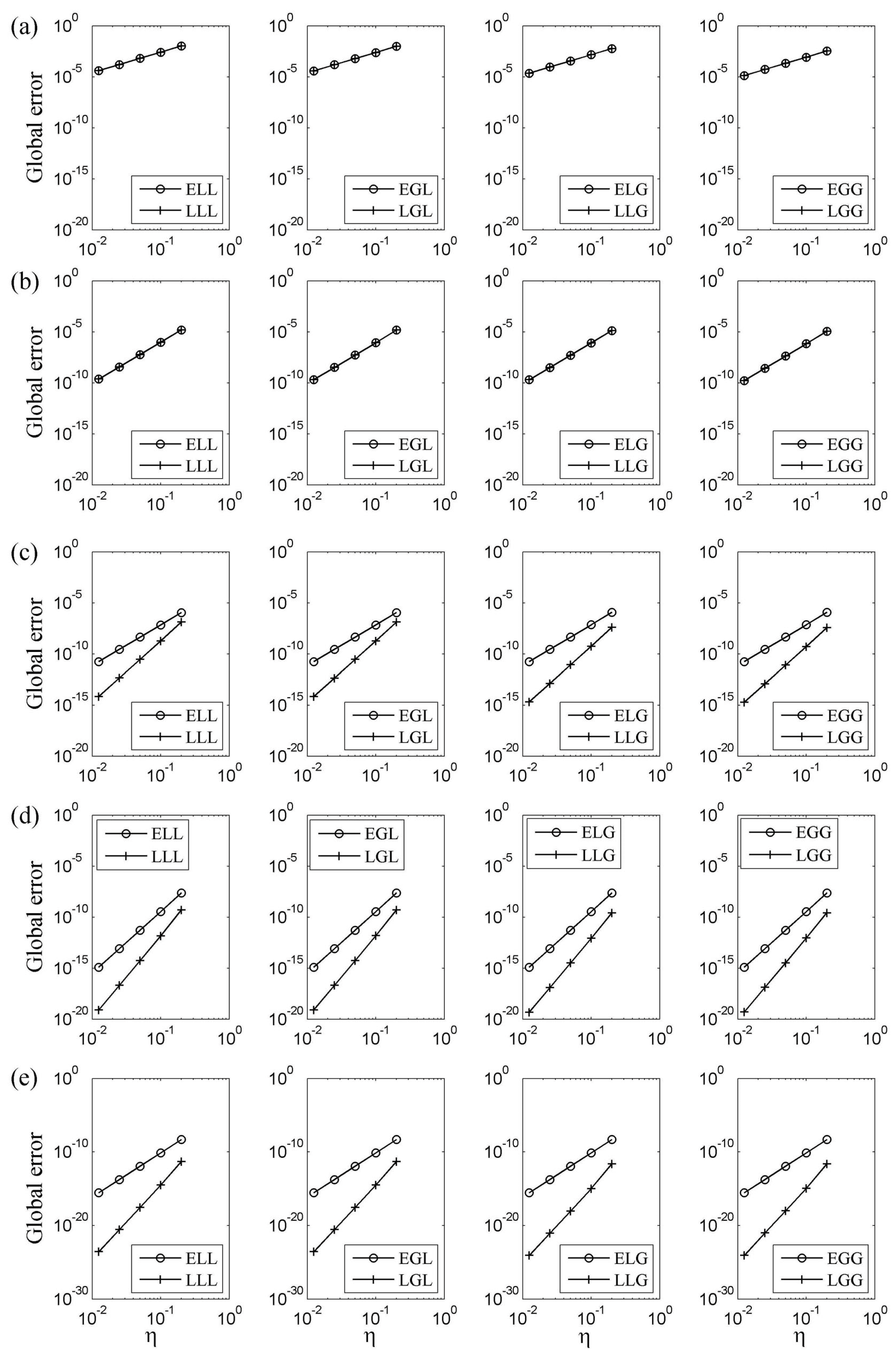
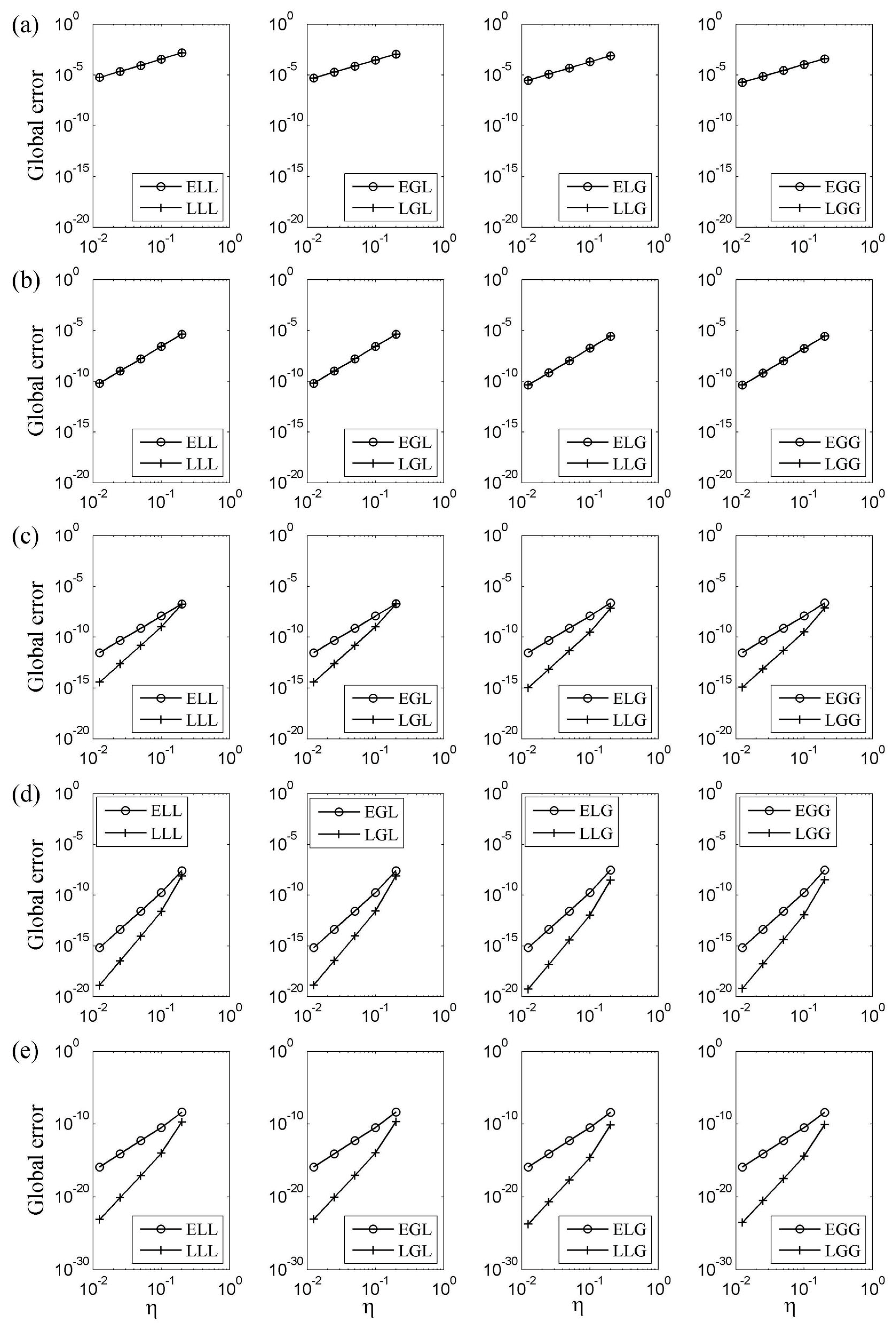
To discover the influence of the control points on the algorithms, we divide eight algorithms into four groups. Group A includes ELL and LLL, group B includes EGL and LGL, group C includes ELG and LLG, and group D includes EGG and LGG. The two algorithms in the same group follow the same quadrature rule but different control points, since evidently the different precision between the two algorithms is determined by the type of control points. Figure 2 shows the log-log plot of the global error of the Hamiltonian during time $0~400s$, where rows (a)–(e) correspond to $m=2,3,\cdots ,6$, respectively. The first column corresponds to group A, the second column corresponds to group B, the third column corresponds to group C, and the fourth column corresponds to group D. When $m=2$ or 3, the equidistant points and Lobatto points are located on the same position, which means that the two algorithms in each group are constructed by the same quadrature rule and the same control points. That is, they are identical; thus, the two curves are coincidental in rows (a) and (b). When $m>3$, the equidistant points and Lobatto points are not located on the same position anymore, and the differences of control points can lead to different precisions. By comparing the two algorithms of each group, we found that, for a given $m$, the algorithm using Lobatto control points always has a higher order than those that use equidistant control points.

The numerically determined order for the eight algorithms is summarized in

Table 3. Numerical convergence order of the eight algorithms.

$m$	2	3	4	5	6	7	8	9
$s$ (EGG, EGL, ELG, ELL)	2	4	4	6	6	8	8	10
$s$ (LGG, LGL, LLG, LLL)	2	4	6	8	10	12	14	16

. For the algorithms LGG, LGL, LLG and LLL that use Lobatto control points, their orders are $s=2m-2$. For the algorithms EGG, EGL, ELG and ELL that use equidistant control points, their order satisfies

$$s=\{\begin{array}{l}m,\hspace{1em}\hspace{1em}m\mathrm{is}\mathrm{even}\\ m+1,m\mathrm{is}\mathrm{odd}\end{array}$$

(53)

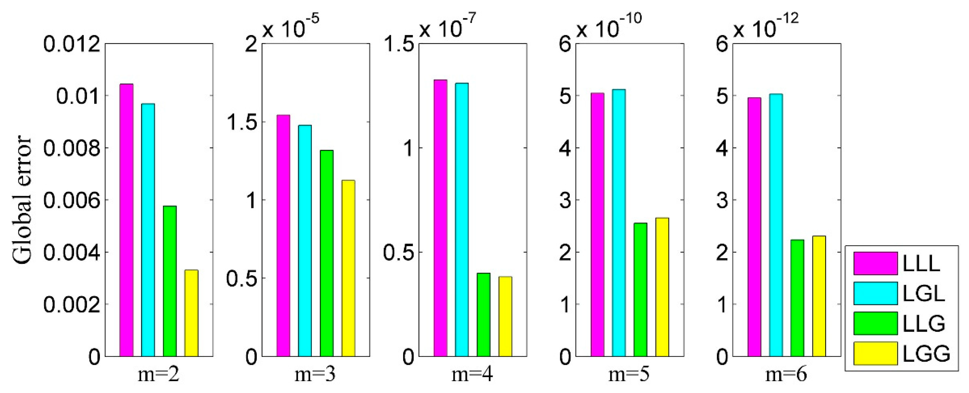
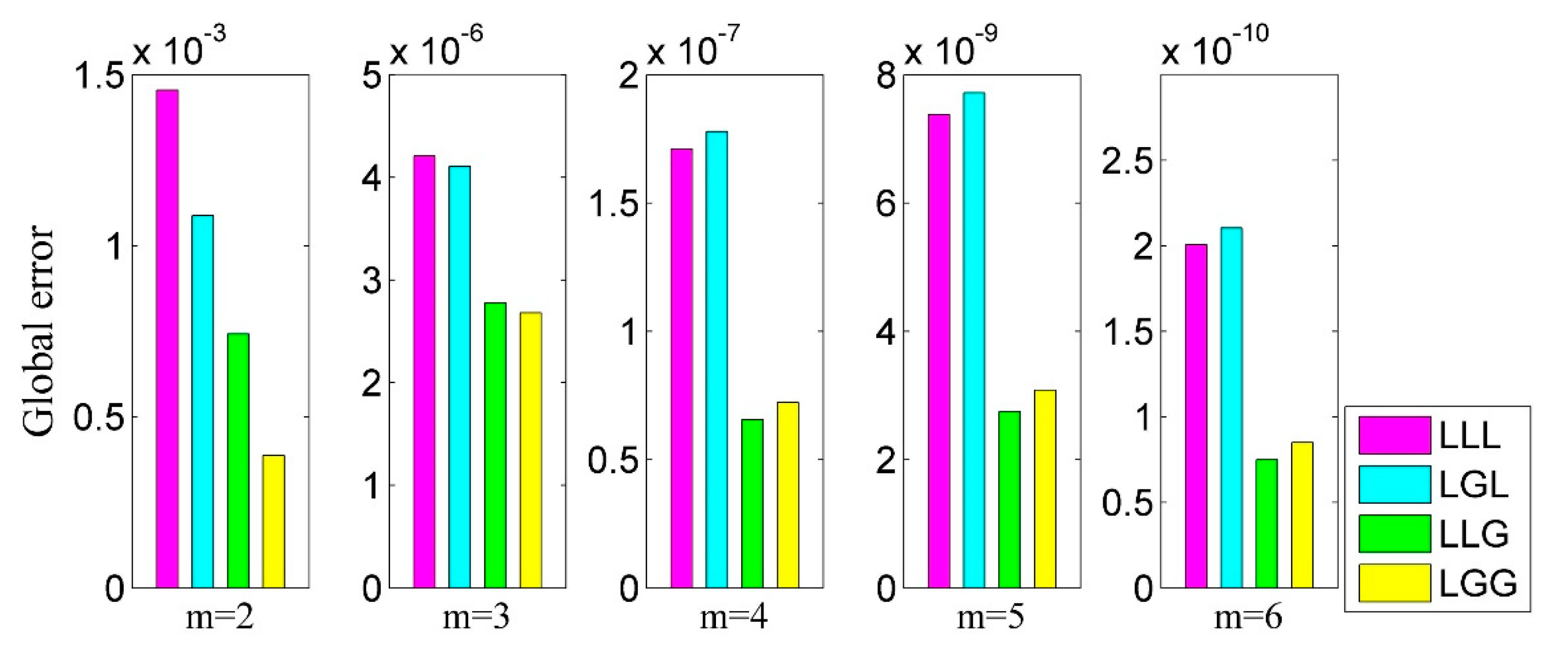
Therefore, the Lobatto control points should be selected to obtain a higher order. Next, to assess the influence of the quadrature rules on the algorithm, LLL, LGL, LLG and LGG are further studied. Figure 3 shows the global errors of Hamiltonian of LLL, LGL, LLG and LGG for $m=2,3,\cdots ,6$ and time step $\eta =0.1$. Firstly, it shows that the global error of LGG is always better that LLL. This means that, when the control points are given, using the Gauss–Legendre quadrature rule for both the unconstrained term and the constrained term will achieve higher precision than using the Lobatto quadrature rule. Furthermore, the global errors of LLL and LGL are basically the same, as are the global errors of LLG and LGG. This outcome means that only changing the quadrature rule of the unconstrained term has little effect on the precision of the algorithms, and the influence of the quadrature rules on the precision of the algorithm is mainly through the constrained term.

In order to evaluate the computational efficiency, we made a comparison between our method and the constrained Lobatto IIIA–IIIB partitioned Runge–Kutta method. When the number of points is $m$, our method is a system of $md+mc$ equations, while the constrained Lobatto IIIA–IIIB partitioned Runge–Kutta method is a system of $2md+\left(m-2\right)c$ equations. As the dimension of generalized coordinates is generally greater than the number of holonomic constraints, i.e., $d>c$, the number of equations of our method is generally less than the constrained Lobatto IIIA–IIIB partitioned Runge–Kutta method. Meanwhile, according to [38], when choosing Lobatto points as control points and the Lobatto quadrature rule for both unconstrained item and constrained item, the associated algorithm LLL has the same precision as the constrained Lobatto IIIA–IIIB partitioned Runge–Kutta method. This means that, compared with the constrained Lobatto IIIA–IIIB partitioned Runge–Kutta method, algorithms LLG and LGG have higher precision while taking less computational time.

4.3. Example 2: The Triple Pendulum

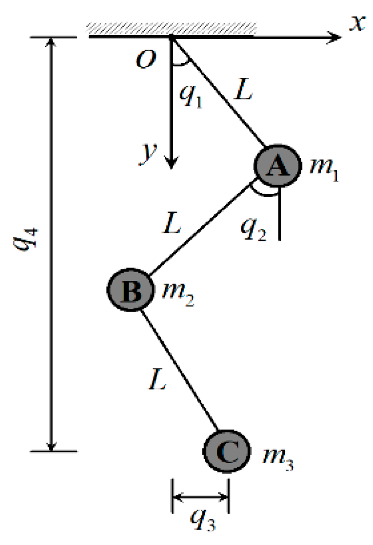
In this section, the triple pendulum is taken to reconfirm the conclusions in Section 4.2. The coordinate selection method of the triple pendulum is shown in Figure 4. The Lagrangian and constraints are given by

$$\begin{array}{cc}L& =\frac{1}{2}{m}_1{L}^2{\dot{q}}_1^2+\frac{1}{2}{m}_2{L}^2\left({\dot{q}}_1^2+{\dot{q}}_2^2+2{\dot{q}}_1{\dot{q}}_2\cos \left(q_1-q_2\right)\right)+\hfill \\ \hfill & \frac{1}{2}{m}_3\left({\dot{q}}_3^2+{\dot{q}}_4^2\right)+m_{1}gL\cos q_1+m_{2}gL\cos q_1+m_{2}gL\cos q_2+m_{3}g{q}_4\end{array}$$

(54)

$$g\left(q\right)={\left(q_3-L\left(\sin q_1+\sin q_2\right)\right)}^2+{\left(q_4-L\left(\cos q_1+\cos q_2\right)\right)}^2-L^2=0$$

(55)

In this paper, $m_1=m_2=m_3=L=g=1$ is used, and the initial conditions are given by

$$q\left(0\right)={\left\{0,0,\sqrt{2}/2,2+\sqrt{2}/2\right\}}^{\mathrm{T}},\hspace{1em}\dot{q}\left(0\right)=0$$

(56)

The log-log plot of the global error of the triple pendulum is shown in Figure 5, which shows that algorithms using Lobatto control points have higher orders than those using equidistant control points. The comparison of the global error of Hamiltonian of LLL, LGL, LLG and LGG is given in Figure 6, which shows that LGG has the best precision between the three algorithms. In fact, several other examples are tested and verified, and the results agree well with the nonlinear spring pendulum and the triple pendulum.

4.4. Example 3: Six Balls

In this section, we show the long-time energy behaviors, the conservation of angular momentum and the structure-preserving properties through a numerical example.

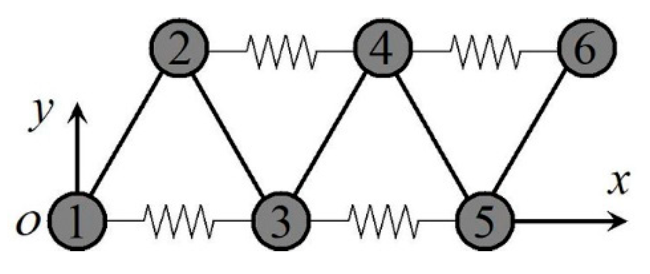
Consider a system of six balls [16] with the configuration shown in Figure 7. The natural lengths of the springs and the lengths of the rigid bars are 1. The balls are numbered 1 to 6, and the number i-th ball has mass $m_i$, generalized coordinates $\left(x_i,y_i\right)$ and momentum $\left(p_{ix},p_{iy}\right)$. The Lagrangian and constraints are given by

$$L=\frac{1}{2}{\displaystyle \sum _{i=1}^6\left({\dot{x}}_i^2+{\dot{y}}_i^2\right)}-\frac{1}{2}{\displaystyle \sum _{i=1}^4{\left(\sqrt{{\left(x_{i+2}-x_i\right)}^2+{\left(y_{i+2}-y_i\right)}^2}-1\right)}^2}$$

(57)

$$g_i\left(q\right)={\left(x_{i+1}-x_i\right)}^2+{\left(y_{i+1}-y_i\right)}^2-1=0,\hspace{1em}\hspace{1em}i=1,2,\cdots ,5$$

(58)

In this paper, the following initial condition is used:

$$\begin{array}{l}q\left(0\right)={\left\{\frac{1-\sqrt{2}}{2},\frac{\sqrt{3}-\sqrt{2}}{2},\frac{1}{2},\frac{\sqrt{3}}{2},1,0,\frac{3}{2},\frac{\sqrt{3}}{2},2,0,2+\frac{\sqrt{2}}{2},\frac{\sqrt{2}}{2}\right\}}^{\mathrm{T}}\\ \dot{q}\left(0\right)=0\end{array}$$

(59)

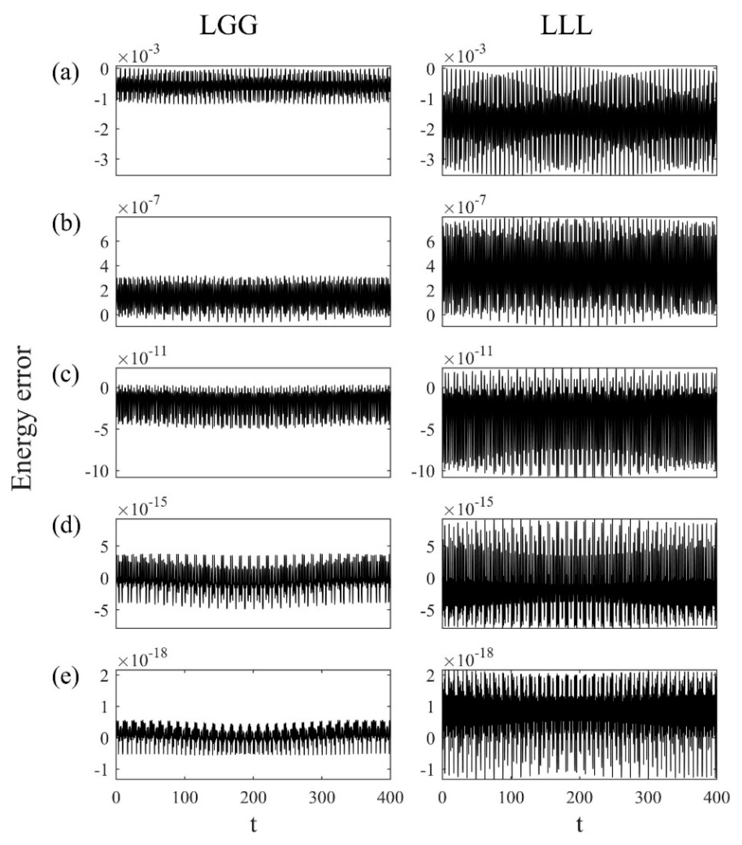
The symplectic algorithm has good long-time energy behavior. Figure 8 shows the energy error of LGG and LLL for $m=2,3,\cdots ,6$ with a long-time duration of $0\sim 400s$. It shows that the energy errors of both algorithms have definite upper and lower bounds and will not increase or decrease even after a long-time simulation.

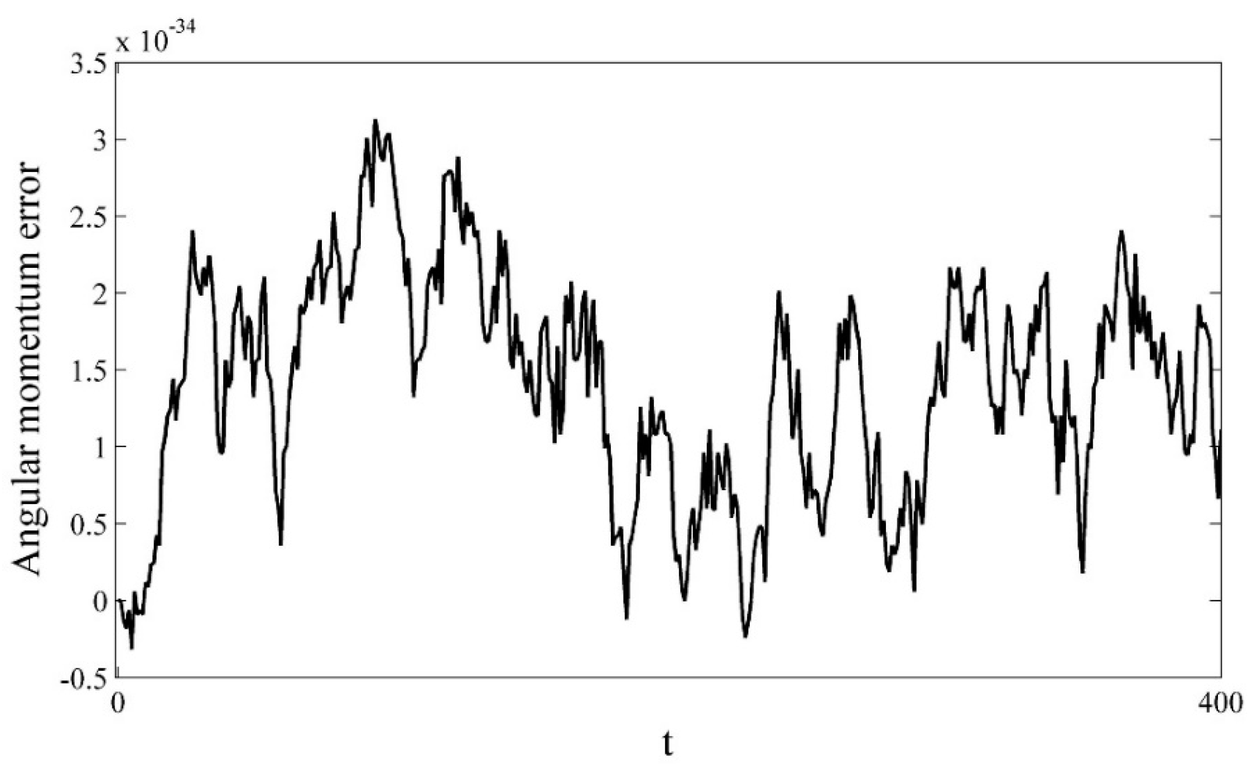
For the six balls problem, the angular momentum

$$I\left(q,p\right)={\displaystyle \sum _{i=1}^6\left(-p_{ix}{y}_i+p_{iy}{x}_i\right)}$$

(60)

is a conserved quantity based on the discrete Noether theorem for the constrained system [4]. Figure 9 shows the error of angular momentum of LGG with $\eta =1$ and $m=2$. It shows that the angular momentum attains numerical accuracy, even when using a large step and a low order.

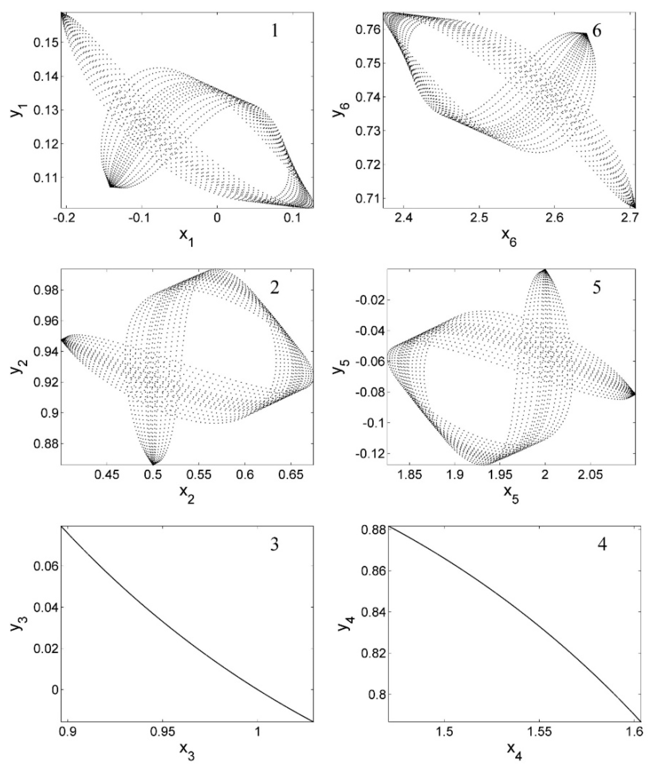
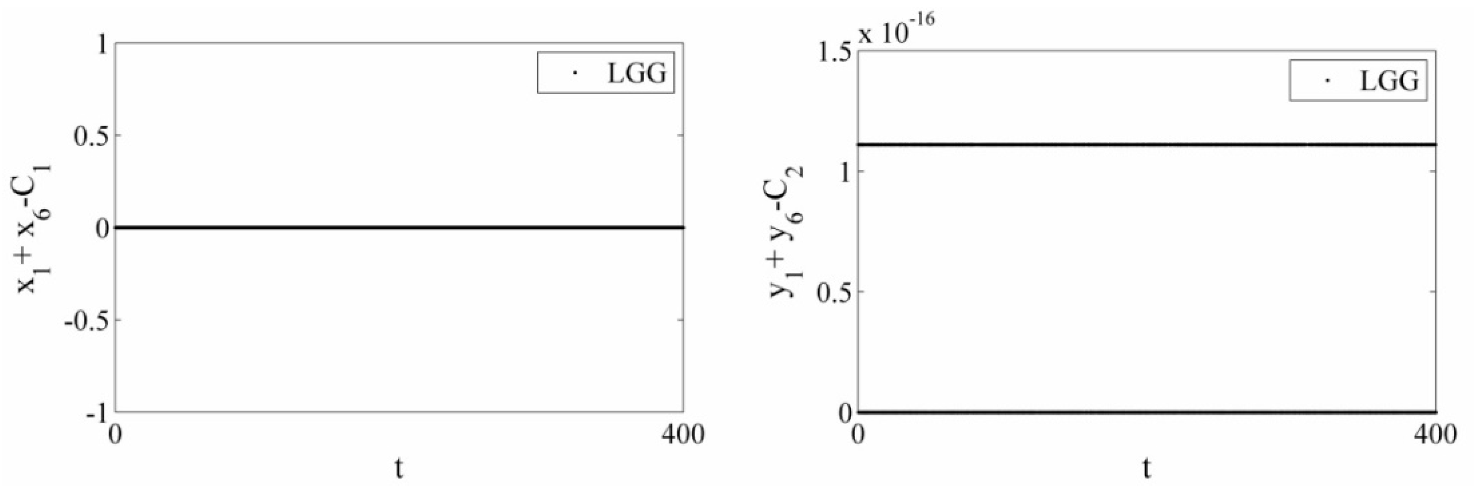
The variational integrator can inherit the specific properties of the underlying mechanical system. The trajectory of the six balls is shown in Figure 10 as simulated by LGG during the time $300\sim 400s$ with $m=2$ and time step $\eta =0.1$, which shows that antisymmetric is an inherent property of this system. For example, considering ball 1 and ball 6, due to their antisymmetric property, their generalized coordinates satisfy

$$x_1+x_6-C_1=0,\hspace{1em}\hspace{1em}{y}_1+y_6-C_2=0$$

(61)

in which $C_1$ and $C_2$ are constant. Figure 11 shows the value of Equation (61) during the time $0\sim 400s$ as simulated by LGG. It shows that, even after long-time simulations, the antisymmetric property is still perfectly conserved.

5. Conclusions

New variational integrators for dynamics with holonomic constraints are proposed in this paper based on the Galerkin variational integrators. The augmented Lagrangian is split into two parts, the position of quadrature points used by two parts of the integral are both independent of the position of the control points. Then, eight algorithms are practically constructed using different control points and quadrature rules. Based on these eight algorithms, the influence of control points and quadrature points on the accuracy of the algorithm is discussed in detail using numerical examples. Firstly, the numerical results show that the type of control point will influence the order of the algorithms, i.e., using Lobatto control points will achieve a higher order than using equidistant control points. The order obtained by the Lobatto control points is $s=2m-2$, and the order of the equidistant control points follows Equation (53). On the other hand, quadrature rules will influence the global error of the algorithms: using Gauss–Legendre quadrature rules will achieve better precision than using Lobatto quadrature rules, and the influence of quadrature rules on the precision of the algorithm is mainly through the constrained term.

References

- Hairer, E.; Nørsett, S.P.; Wanner, G. Solving Ordinary Differential Equations I: Nonstiff Problems; Springer: Berlin, Germany, 1993. [Google Scholar]
- Hairer, E.; Wanner, G. Solving Ordinary Differential Equations II: Nonstiff Problems; Springer: Berlin, Germany, 1996. [Google Scholar]
- Reich, S. Momentum conserving symplectic integrators. Phys. D Nonlinear Phenom. 1994, 76, 375–383. [Google Scholar] [CrossRef] [Green Version]
- Marsden, J.E.; West, M. Discrete mechanics and variational integrators. Acta Numer. 2001, 10, 357–514. [Google Scholar] [CrossRef] [Green Version]
- Hairer, E.; Lubich, C.; Wanner, G. Geometric Numerical Integration: Structure-Preserving Algorithms for Ordinary Differential Equations; Springer: Berlin/Heidelberg, Germany, 2006. [Google Scholar]
- Enyi, C. Sobolev Spaces and Variational Methods Applied to Elliptic PDE’s; LAP Lambert Academic Publishing: Saarbrücken, Germany, 2012. [Google Scholar]
- Scapellato, A. New Perspectives in the Theory of Some Function Spaces and their Applications. In Proceedings of the AIP Conference, International Conference of Numerical Analysis and Applied Mathematics (ICNAAM 2018), Rhodes, Greece, 13–18 September 2018; Volume 1978, p. 140002. [Google Scholar] [CrossRef]
- Jordan, B.W.; Polak, E. Theory of a Class of Discrete Optimal Control Systems. Int. J. Electron. 1964, 17, 697–711. [Google Scholar] [CrossRef]
- Hwang, C.L.; Fan, L.T. A Discrete Version of Pontryagin’s Maximum Principle. Oper. Res. 1967, 15, 139–146. [Google Scholar] [CrossRef]
- Cadzow, J.A. Discrete calculus of variations. Int. J. Control 1970, 11, 393–407. [Google Scholar] [CrossRef]
- Logan, J.D. First integrals in the discrete variational calculus. Aequ. Math. 1973, 9, 210–220. [Google Scholar] [CrossRef]
- Maeda, S. Canonical structure and symmetries for discrete systems. Math. Jpn. 1980, 25, 405–420. [Google Scholar]
- Lee, T.D. Difference equations and conservation laws. J. Stat. Phys. 1987, 46, 843–860. [Google Scholar] [CrossRef]
- Jean-Paul, R.; Giovanni, C.; Berendsen, H.J.C. Numerical integration of the cartesian equations of motion of a system with constraints: Molecular dynamics of n-alkanes. J. Comput. Phys. 1977, 23, 327–341. [Google Scholar]
- Andersen, H.C. Rattle: A velocity version of the shake algorithm for molecular dynamics calculations. J. Comput. Phys. 1983, 52, 24–34. [Google Scholar] [CrossRef] [Green Version]
- Leimkuhler, B.J.; Skeel, R.D. Symplectic Numerical Integrators in Constrained Hamiltonian Systems; Academic Press Professional, Inc.: Cambridge, MA, USA, 1994. [Google Scholar]
- Skeel, R.D.; Zhang, G.; Schlick, T. A Family of Symplectic Integrators: Stability, Accuracy, and Molecular Dynamics Applications. Siam J. Entific Comput. 1997, 18, 203–222. [Google Scholar] [CrossRef]
- Reich, S. Multi-Symplectic Runge–Kutta Collocation Methods for Hamiltonian Wave Equations. J. Comput. Phys. 2000, 157, 473–499. [Google Scholar] [CrossRef] [Green Version]
- Blackmore, D.; Prykarpatsky, A.K.; Samoylenko, V.H. Nonlinear Dynamical Systems of Mathematical Physics: Spectral and Symplectic Integrability Analysis; World Scientific: Singapore, 2011. [Google Scholar]
- Lew, A.; Marsden, J.; Ortiz, M.; West, M. Variational time integrators. Int. J. Numer. Methods Eng. 2004, 60, 153–212. [Google Scholar] [CrossRef] [Green Version]
- Lall, S.; West, M. Discrete variational Hamiltonian mechanics. J. Phys. A Math. Gen. 2006, 39, 5509–5519. [Google Scholar] [CrossRef] [Green Version]
- Leok, M. Discrete Hamiltonian variational integrators. Ima J. Numer. Anal. 2011, 31, 1497–1532. [Google Scholar] [CrossRef] [Green Version]
- Marsden, J.E.; Patrick, G.W.; Shkoller, S. Multisymplectic geometry, variational integrators, and nonlinear PDEs. Commun. Math. Phys. 1998, 199, 351–395. [Google Scholar] [CrossRef] [Green Version]
- Lew, A.; Marsden, J.E.; Ortiz, M.; West, M. Asynchronous Variational Integrators. Arch. Ration. Mech. Anal. 2003, 167, 85–146. [Google Scholar] [CrossRef] [Green Version]
- Tyranowski, T.M.; Desbrun, M. R-Adaptive Multisymplectic and Variational Integrators. Mathematics 2019, 7, 642. [Google Scholar] [CrossRef] [Green Version]
- Cortés, J.; Martínez, S. Non-holonomic integrators. Nonlinearity 2001, 14, 1365–1392. [Google Scholar] [CrossRef]
- De León, M.; De Diego, D.M.; Santamaria-Merino, A. Geometric integrators and nonholonomic mechanics. J. Math. Phys. 2004, 45, 1042–1064. [Google Scholar] [CrossRef] [Green Version]
- Fedorov, Y.N.; Zenkov, D.V. Discrete nonholonomic LL systems on Lie groups. Nonlinearity 2005, 18, 2211–2241. [Google Scholar] [CrossRef] [Green Version]
- Kane, C.; Marsden, J.E.; Ortiz, M.; West, M. Variational integrators and the Newmark algorithm for conservative and dissipative mechanical systems. Int. J. Numer. Methods Eng. 2000, 49, 1295–1325. [Google Scholar] [CrossRef]
- Pekarek, D.; Ames, A.D.; Marsden, J.E. Discrete Mechanics and Optimal Control Applied to the Compass Gait Biped. In Proceedings of the 46th IEEE Conference on Decision & Control, New Orleans, LA, USA, 12–14 December 2007. [Google Scholar]
- Campos, C.M.; Ober-Bloebaum, S.; Trelat, E. High order variational integrators in the optimal control of mechanical systems. Discret. Contin. Dyn. Syst. 2015, 35, 4193–4223. [Google Scholar] [CrossRef] [Green Version]
- De Leon, M.; Martin De Diego, D.; Santamaria-Merino, A. Discrete variational integrators and optimal control theory. Adv. Comput. Math. 2007, 26, 251–268. [Google Scholar] [CrossRef] [Green Version]
- Ruggieri, M.; Valenti, A. Symmetries and reduction techniques for dissipative models. J. Math. Phys. 2009, 50. [Google Scholar] [CrossRef]
- Limebeer, D.J.N.; Ober-Blobaum, S.; Farshi, F.H. Variational Integrators for Dissipative Systems. IEEE Trans. Autom. Control 2020, 65, 1381–1396. [Google Scholar] [CrossRef]
- Burnett, C.L.; Holm, D.D.; Meier, D.M. Inexact trajectory planning and inverse problems in the Hamilton-Pontryagin framework. Proc. R. Soc. A Math. Phys. Eng. Sci. 2013, 469. [Google Scholar] [CrossRef]
- Colombo, L.; Martin de Diego, D. Higher-Order variational problems on lie groups and optimal control applications. J. Geom. Mech. 2014, 6, 451–478. [Google Scholar] [CrossRef]
- Crouch, P.; Leite, F.S. The dynamic interpolation problem: On Riemannian manifolds, Lie groups, and symmetric spaces. J. Dyn. Control Syst. 1995, 1, 177–202. [Google Scholar] [CrossRef]
- Wenger, T.; Ober-Blobaum, S.; Leyendecker, S. Construction and analysis of higher order variational integrators for dynamical systems with holonomic constraints. Adv. Comput. Math. 2017, 43, 1163–1195. [Google Scholar] [CrossRef]
- Hall, J.; Leok, M. Spectral variational integrators. Numer. Math. 2015, 130, 681–740. [Google Scholar] [CrossRef]
- Leok, M.; Shingel, T. General techniques for constructing variational integrators. Front. Math. China 2012, 7, 273–303. [Google Scholar] [CrossRef] [Green Version]
- Ober-Bloebaum, S.; Saake, N. Construction and analysis of higher order Galerkin variational integrators. Adv. Comput. Math. 2015, 41, 955–986. [Google Scholar] [CrossRef]
Figure 1.
Nonlinear spring-pendulum.
Figure 2.
Nonlinear spring pendulum: Log-log plot of the global error of Hamiltonian during with (a–e) corresponding to , respectively.
Figure 3.
Nonlinear spring pendulum: Global error of Hamiltonian of LLL, LGL, LLG and LGG with and time step .
Figure 4.
Triple pendulum.
Figure 5.
Triple pendulum: Log-log plot of the global error of Hamiltonian during with (a–e) corresponding to , respectively.
Figure 6.
Triple pendulum: Global error of Hamiltonian of LLL, LGL, LLG and LGG with and time step .
Figure 7.
Six balls.
Figure 8.
Six balls: Energy error of LGG and LLL with (a–e) corresponding to , respectively.
Figure 9.
Six balls: Angular momentum error of LGG with time step and .
Figure 10.
The trajectory of the six balls of the LGG algorithm during the time with and .
Figure 11.
Six balls: Antisymmetric property of the generalized coordinates