Software Reliability Model with Dependent Failures and SPRT

1
Department of Computer Science and Statistics, Chosun University, 309 Pilmun-daero, Dong-gu, Gwangju 61452, Korea
2
Department of Industrial and Systems Engineering, Rutgers University, 96 Frelinghuysen Road, Piscataway, NJ 08855-8018, USA
*
Authors to whom correspondence should be addressed.
Mathematics 2020, 8(8), 1366; https://0-doi-org.brum.beds.ac.uk/10.3390/math8081366
Submission received: 13 July 2020
/
Revised: 30 July 2020
/
Accepted: 13 August 2020
/
Published: 14 August 2020
Abstract
:Software reliability and quality are crucial in several fields. Related studies have focused on software reliability growth models (SRGMs). Herein, we propose a new SRGM that assumes interdependent software failures. We conduct experiments on real-world datasets to compare the goodness-of-fit of the proposed model with the results of previous nonhomogeneous Poisson process SRGMs using several evaluation criteria. In addition, we determine software reliability using Wald’s sequential probability ratio test (SPRT), which is more efficient than the classical hypothesis test (the latter requires substantially more data and time because the test is performed only after data collection is completed). The experimental results demonstrate the superiority of the proposed model and the effectiveness of the SPRT.
1. Introduction
Software performance and reliability are essential in various fields, such as the Internet of Things. If software reliability is not guaranteed, economic and human losses may occur. Hence, various studies have been conducted to improve software reliability and prevent loss.
Software reliability growth models (SRGMs) are tools that estimate the quality and reliability of software products. SRGMs not only provide information regarding software reliability for developers and consumers, but also help establish an optimal release policy.
Most SRGMs assume that the mean value function, m(t), is a nonhomogeneous Poisson process (NHPP). The m(t) of each model is a single function that reflects the failure intensity, failure detection, number of remaining failures, and the environment. In particular, assumptions regarding the test and development environments are essential; furthermore, the parameters and the form of depend on the assumptions regarding the environment.
Previous studies have considered the types of fault detection functions and the shape of m(t). The Goel–Okumoto (GO) model [1] is a basic stochastic NHPP SRGM that has inspired several researchers. Ohba et al. [2] proposed an inflection S-shaped curve model. Yamada [3] developed a similar delayed model. Pham et al. [4] reported a nondecreasing inflection S-shaped model with an error introduction rate as an exponential function; the model is known as the Pham–Zhang (PZ) model. Moreover, Pham et al. [5] proposed a generalized NHPP software model that reflected the testing coverage. Subsequently, researchers became interested in environmental factors. In particular, many studies have focused on uncertain operating or testing environments [6,7,8,9,10,11,12,13]. Some recent research has been studied on SRGMs with considerations of time-dependent fault detection [14,15,16,17,18,19], random operating environments [20,21], and multi release software [22,23,24].
Recent studies combined deep learning and machine learning with software reliability [25,26,27,28]. Wang et al. discussed an optimal release policy and the selection of the best software reliability model [28]. Lee et al. proposed an SRGM to consider the actual test time instead of the designed test time [29]. Minamino et al. [30] discussed software reliability and release policies that considered the change-points of data based on the theory of multiproperty utilities. Rani et al. [31] developed a hazard rate model that introduced an imperfect debugging parameter and a single change-point parameter.
Some studies suggest statistical techniques to predict software reliability. Typically, parameters of reliability models are estimated using the least-square estimator (LSE) method. Additionally, the maximum likelihood estimator (MLE) and Bayesian methods have been used [32,33]. However, software reliability models have complex structures and numerous parameters, rendering it difficult to apply the MLE and Bayesian methods; hence, we used the LSE to estimate the parameters in this study.
We applied the sequential probability ratio test (SPRT), a statistical test technique, to efficiently determine software reliability. The SPRT was designed for military and naval equipment development by Wald [34]. The main advantage of a sequential test is that it requires a shorter test time compared with that required by the classical test, which requires a fixed sample size. In addition, the SPRT can instantly determine software reliability whenever new faults occur. Hence, reliability can be assessed based on the change-points of data. This procedure is described in Section 2.
Software reliability studies using Wald’s SPRT procedure have been conducted continually. Stieber applied the SPRT to an NHPP SRGM for the first time [35]. This method has been applied to various SRGMs in many studies [36,37,38,39,40]. Furthermore, the authors of [38] performed the SPRT using order statistics.
Herein, we propose a new SRGM that assumes interdependent software failures. In Section 2, we discuss the efficiency of the SPRT. The proposed model is described in Section 3. In Section 4, we introduce the criteria and data used in the experiments. Subsequently, we discuss the results in Section 5. Finally, Section 6 concludes the paper.
2. Wald’s SPRT
Wald described the efficiency of the SPRT [34]. The probability ratio is used as a test statistic of the SPRT for testing the null hypothesis against an alternative hypothesis. The test is continued (until the next decision) if the following condition is satisfied:
where and are constants used to decide the acceptance and rejection of the null hypothesis , respectively. If , then is rejected. If , then is accepted.
Moreover, A and B depend on α and β, as shown in Equations (2)–(5). Here, α and β are type-1 and -2 errors, respectively. In other words, α is the producer’s risk, whereas β is the consumer’s risk.
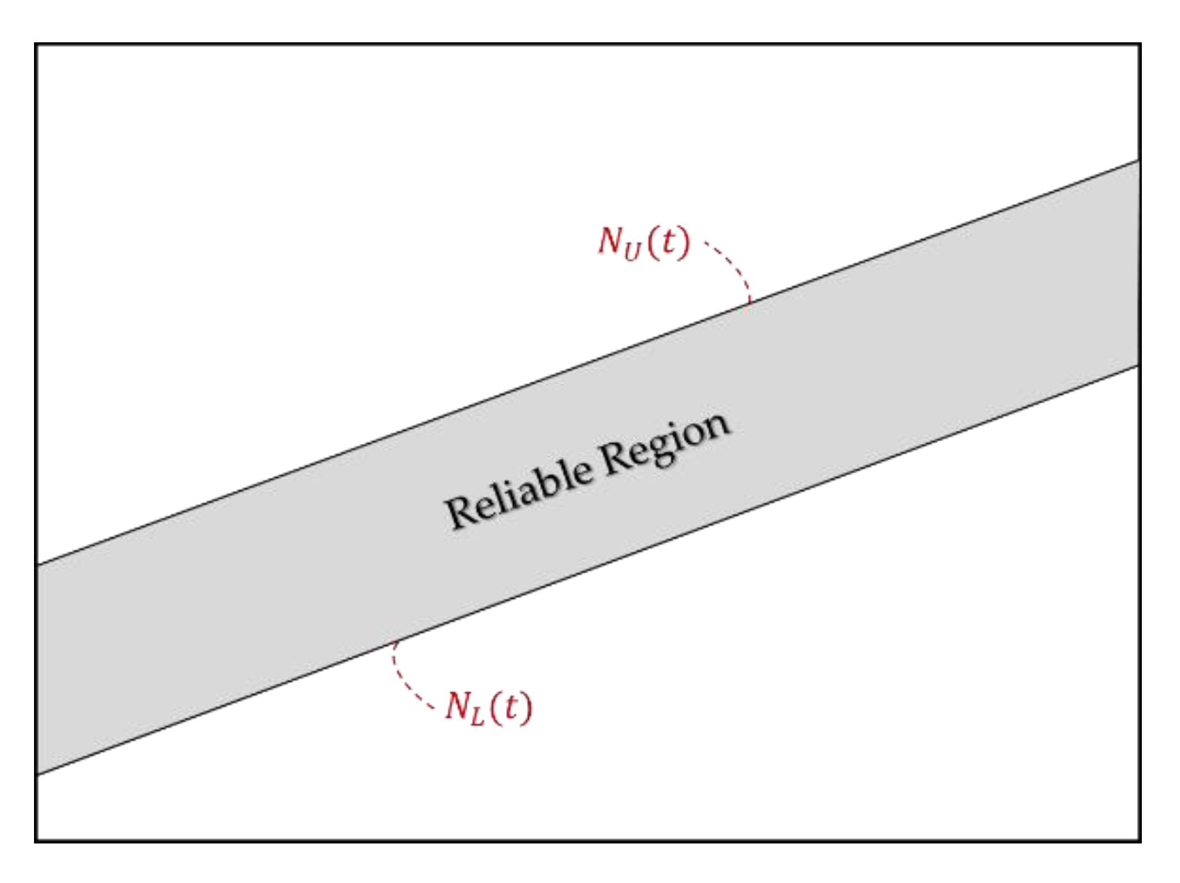
The SPRT can be expressed visually. Figure 1 shows the method to assess software reliability using the SPRT.
In Figure 1, and denote the lower and upper limits of the area in which the software is reliable, respectively. Here, is the expected number of failures at time for the NHPP. If is in the reliable region, then the software is reliable.
where , and are expressed as:
Stieber applied the SPRT to an NHPP SRGM [35] with and , where . A general NHPP SRGM is expressed as:
where m(t) indicates the expected number of detected failures until time t, which is described as:
Stieber defined the probability ratio, which is used as a statistic of the SPRT for NHPP SRGMs, as in Equation (1).
Using Equations (3), (5) and (11), we can rewrite Equation (1) as follows:
In Equation (12), the left term is constant B, and the right term is constant A. Moreover, refers to the probability ratio, .
3. New SRGM
A general SRGM that follows the NHPP, as shown in Equation (9), can be obtained by solving the differential equation shown in Equation (13). Function varies according to each assumption as follows:
where is the fault detection rate function. The model assumes independent failures.
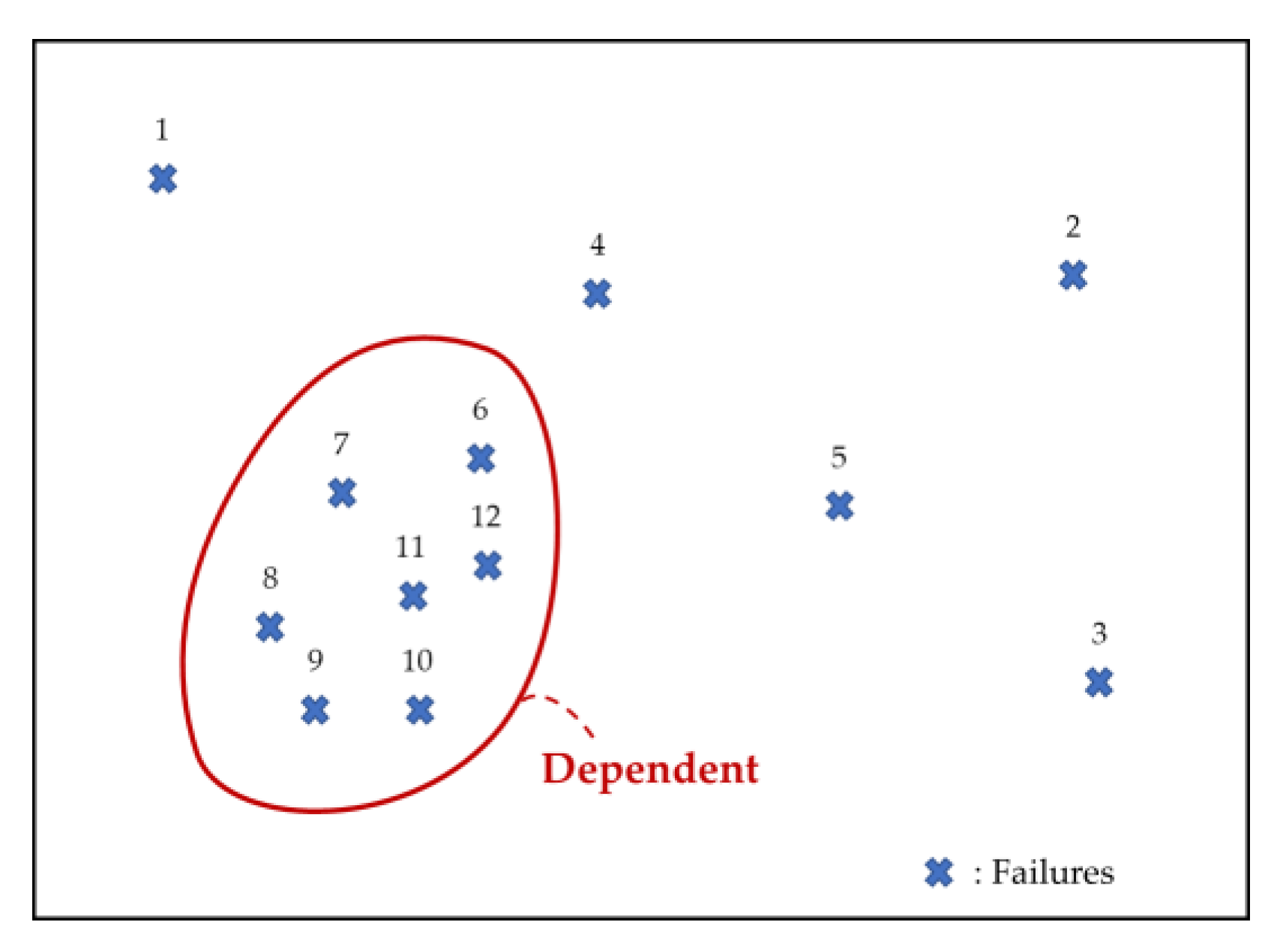
However, the proposed model is different. For example, if a fault occurs because of a syntax error and a developer cannot fix it completely, new faults will be affected. Consequently, failures may depend on one another (Figure 2). Hence, we assume that the failures are dependent. The SRGM based on these assumptions can be obtained from the differential equation expressed in Equation (14).
where and are the functions of the total failure content rate and failure detection rate, respectively. In the proposed model, and are expressed as:
Therefore, we can calculate the of the proposed model. The initial value is .
Table 1 summarizes the m(t) for existing NHPP SRGMs.
4. Experiments
4.1. Criteria
In this section, we elucidate the use of eight criteria to compare the NHPP SRGMs for two real-world datasets.
(1) The mean squared error (MSE) [42] measures the distance between the estimated and actual data, considering the number of observations and the number of parameters in the models. The MSE is defined as follows:
where is the number of total cumulative failures, N the number of model parameters, and the number of cumulative failures at , obtained from the dataset.
(2) The predictive ratio risk (PRR) [42] indicates the distance of model estimates from actual data with respect to the model estimates. It is calculated as:
(3) The predictive power (PP) [43] measures the distance of actual data from the estimate with regard to the actual data. It is defined as:
(4) R-square () [44] is the correlation index of the regression curve equation. It is used to explain the fitting power of the SRGMs and is described as follows:
(5) Akaike’s information criterion (AIC) [45] is used to maximize the likelihood function. It can be considered as an approximate distance from the true probability model, as follows:
where is the degree of freedom. Here, and are written as follows:
(6) The sum of absolute error (SAE) [11] measures the distance between the predicted number of failures and the observed data. It is defined as:
(7) The variation [46] is the standard deviation of the prediction bias. It is expressed as follows:
where bias is expressed as:
(8) The root-mean-square prediction error (RMSPE) [46] estimates the closeness of the predicted values with the actual observations.
The closer the value of is to 1, the better the goodness-of-fit of the dataset. For other criteria, a smaller value indicates a better fit.
4.2. Datasets
Table 2 shows the two datasets used in the experiments. Dataset 1 was collected from a telecommunication system that manages the radio access of wireless systems on a weekly basis [42,47]. It is a test dataset corresponding to two releases of the software. For dataset 1, the number of cumulative failures is at , and the number of total cumulative failures is 26. Dataset 2 includes one of the three releases of weekly medical record system test data that correspond to 188 software tools [42,48]. For dataset 2, the number of cumulative failures is at .
5. Results
5.1. Results of Parameter Estimation and Goodness-of-Fit
Before comparing the fit and applying the SPRT, we estimated the parameters of all models listed in Table 1 using the LSE method. Table 3 summarizes the estimated parameters for datasets.
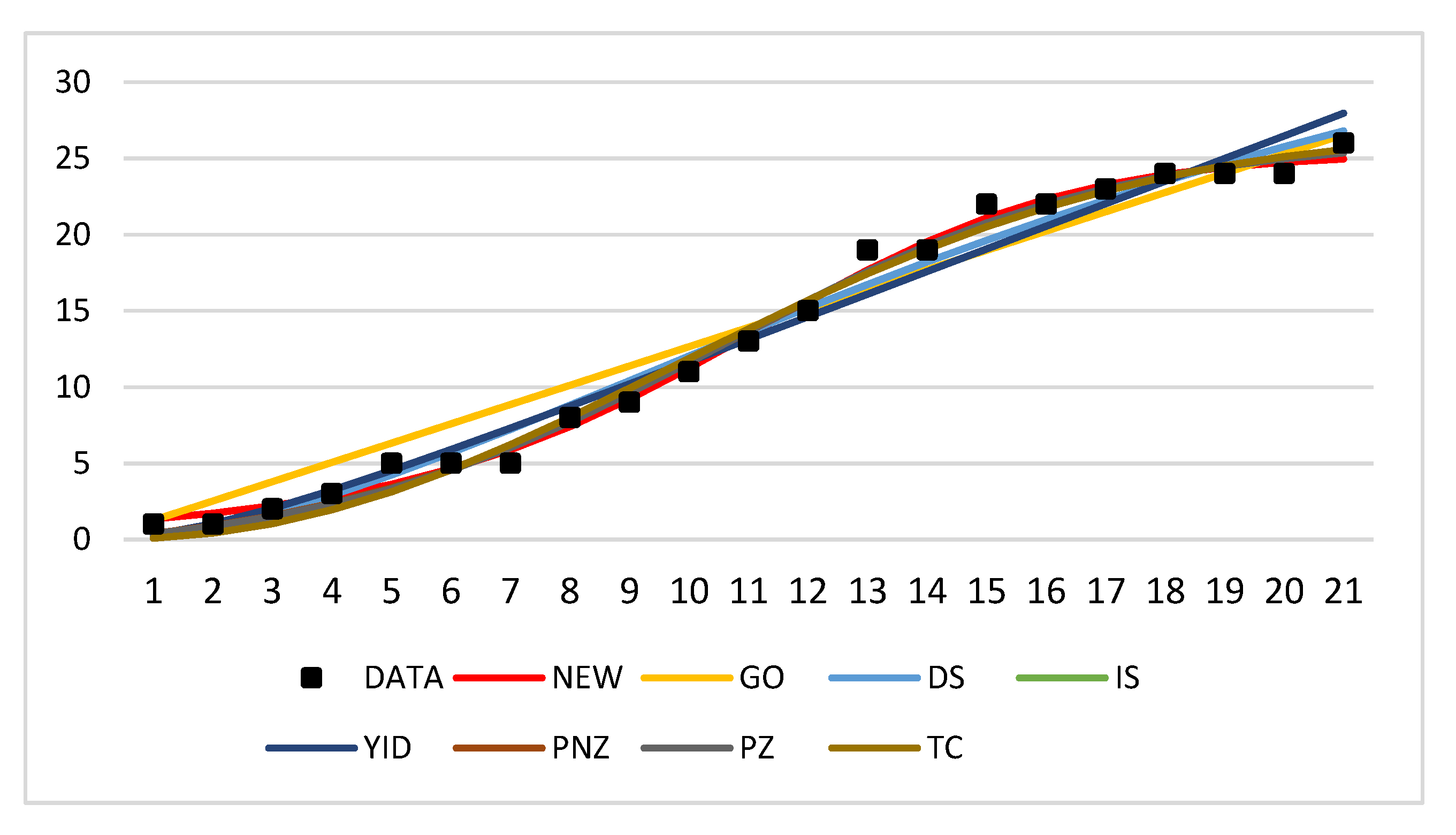
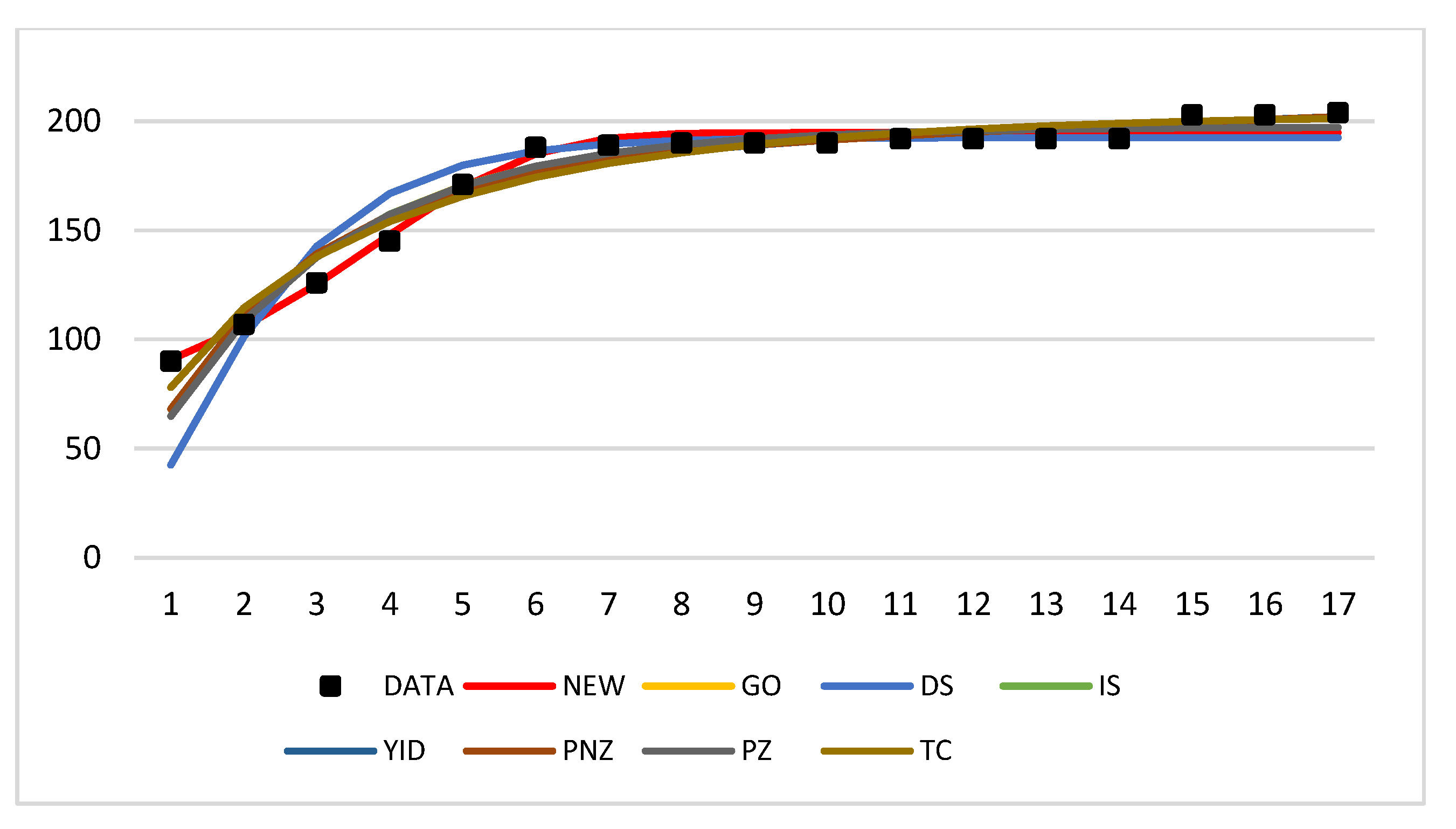
Table 4 and Table 5 present the results for the abovementioned eight criteria of all SRGMs for each dataset. Moreover, Figure 3 and Figure 4 show the m(t).
As shown in Table 4, the proposed model achieved the best results for all criteria except for the PP and AIC. However, the PP and AIC of the proposed model were the third smallest and fifth smallest values, respectively. In general, the proposed model outperformed other models.
As shown in Table 5, the proposed model indicated the best results for most criteria (except for the AIC, variation, and RMSPE). Similarly, the variation and RMSPE of the proposed model were the second smallest values. In general, the proposed model exhibited better fitting than that shown by other models for dataset 2. However, because converged for , the AIC was calculated as not-a-number (NaN). If the AIC of the proposed model was calculated for the time before convergence, , then the value would be 83.51093 (which would be the smallest).
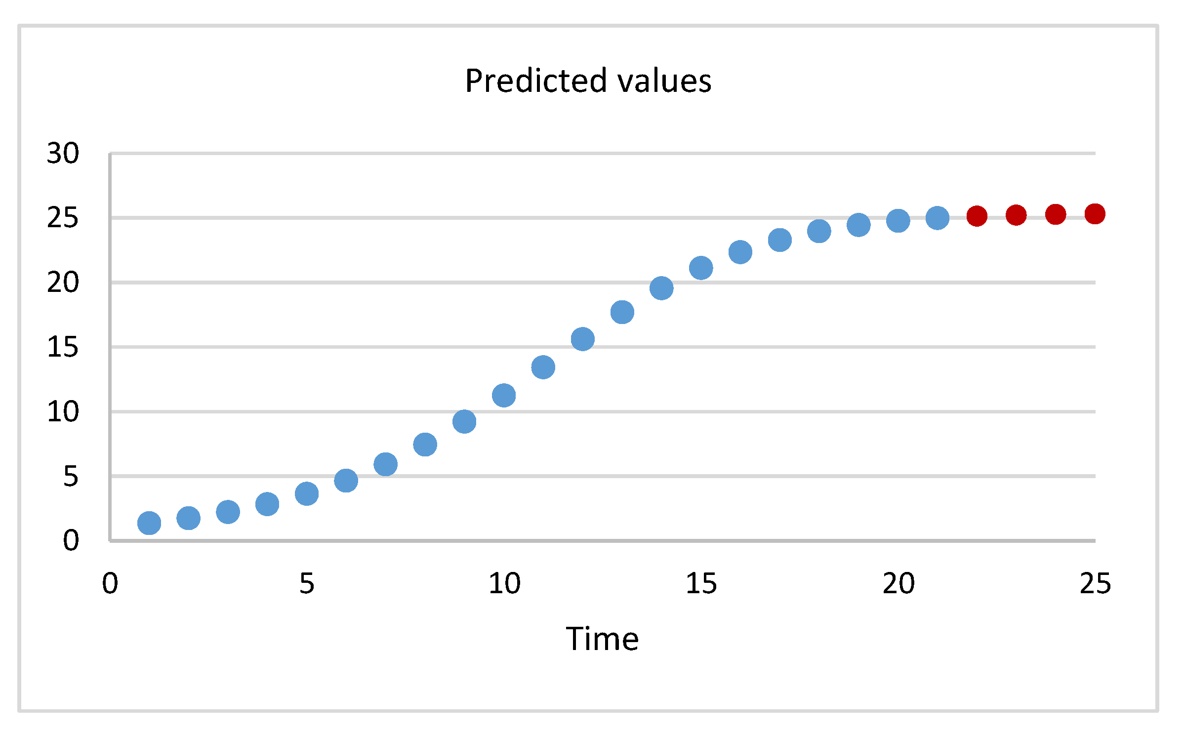
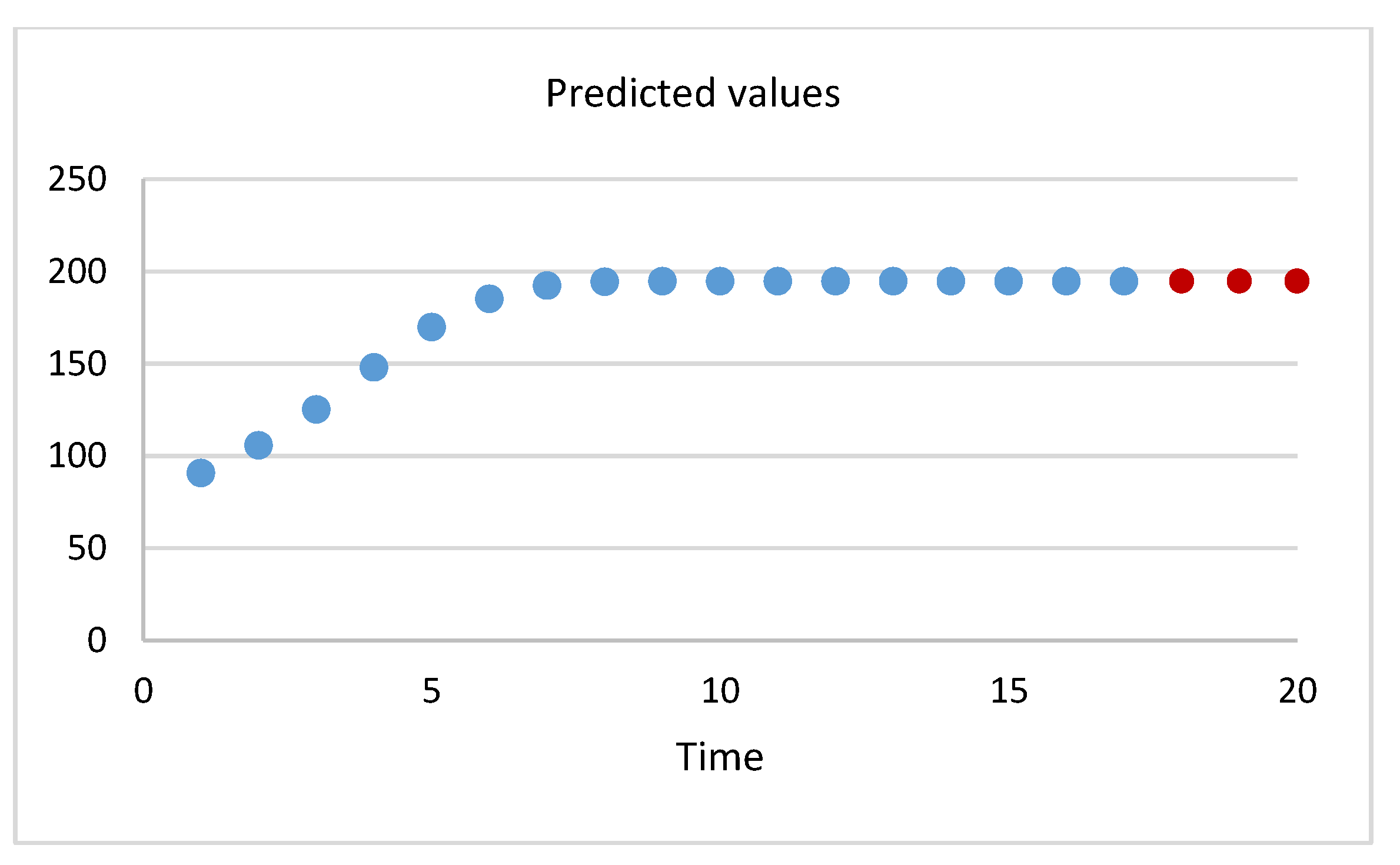
Table 6 and Table 7 and Figure 5 and Figure 6 show the predicted values at for each dataset. The predicted values mean the expected cumulative number of failures by the proposed model. In Table 6, the predicted values for future points are {25.1102, 25.19946, 25.2552, 25.28936} at . In Table 7, the predicted values for future points are {194.766, 194.766, 194.766} at .
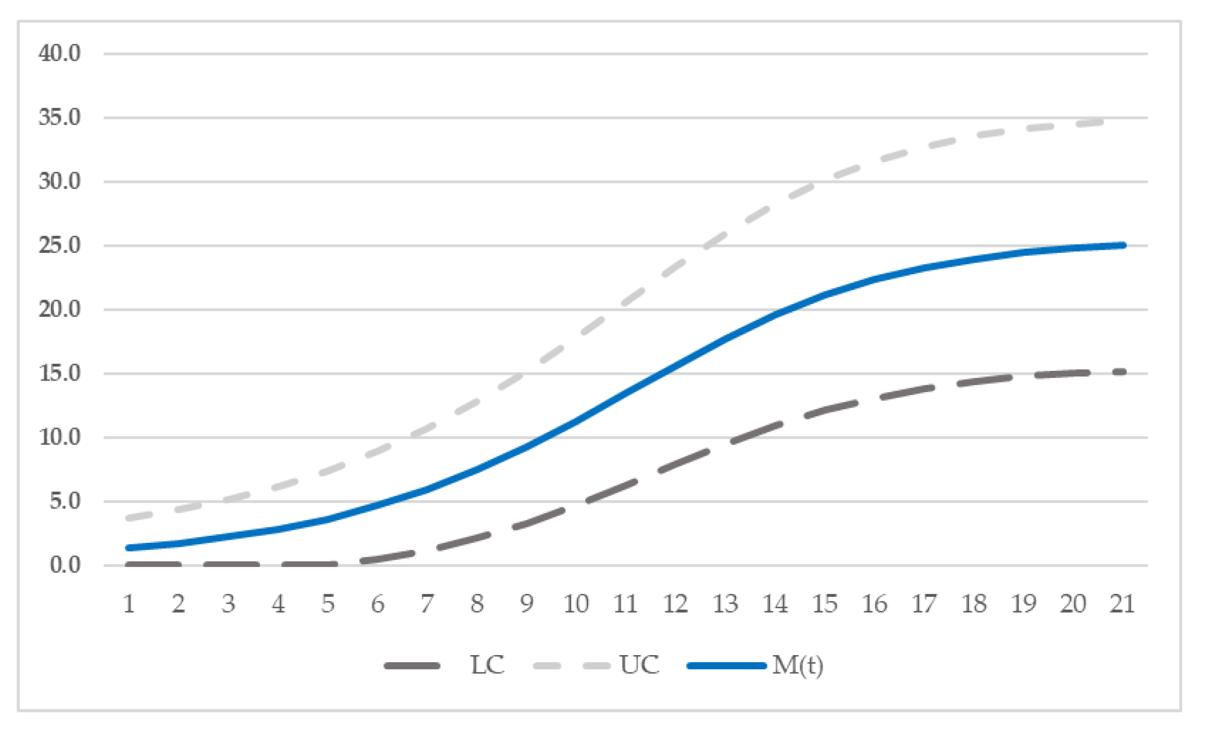
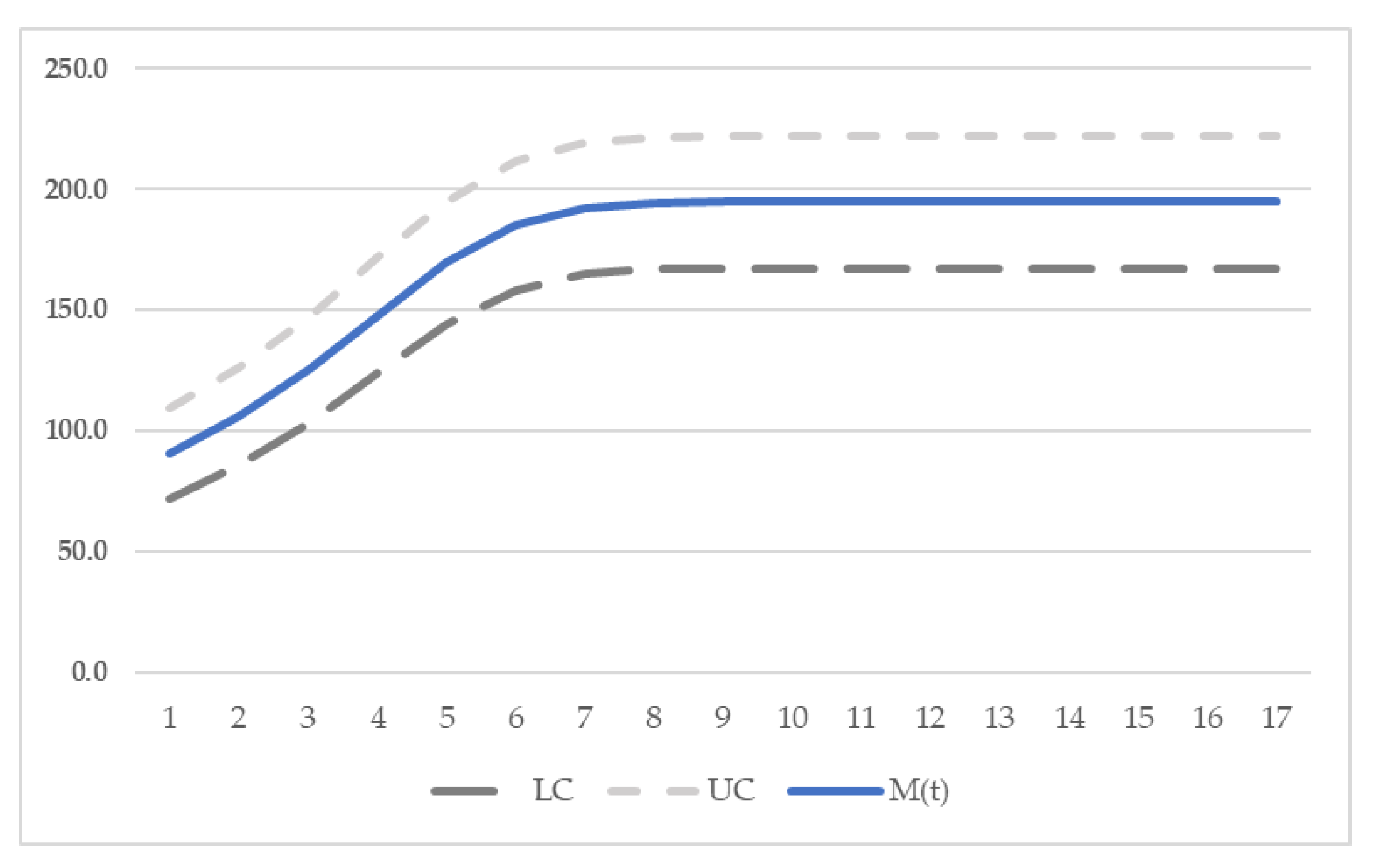
5.2. Confidence Interval
The two-sided limit confidence interval [42] of NHPP SRGMs is defined as:
where is the 100(1) percentile of the standard normal distribution.
5.3. Results of the SPRT for Datasets
We determined the software reliability by applying the SPRT based on the parameters of the proposed model. In particular, a sensitivity analysis showed that and were more sensitive than other parameters of the proposed model; therefore, we focused on and . The related assumptions are listed in Table 9.
Subsequently, we set , for Case 1 and , for Case 2. Substituting and for the of the proposed model instead of , we obtained and , respectively. Likewise, and were obtained by substituting and into , respectively. Substituting and , obtained in Equation (12), allows us to discuss the SPRT procedure.
Table 10 shows the results of the SPRT for parameter for both datasets. Judging the reliability using the proposed model, we conclude that software testing should continue because we cannot determine the software reliability yet.
Table 11 shows the SPRT results for parameter for both datasets. When t = 7 in dataset 1, the test was accepted. Using the proposed model for dataset 2, we conclude that software testing should continue because we cannot determine the software reliability yet. However, as converged for , the result was “Inf”.
6. Conclusions and Remarks
Herein, we proposed a new SRGM. General SRGMs assume independent failures. However, in the proposed model, software failures depend on one another. We presented experiments on real-world datasets using eight evaluation criteria. The proposed model achieved the best goodness-of-fit on both datasets. In addition, we evaluated the software reliability using the SPRT, which is more efficient than the classical hypothesis test. As shown in Table 10, we demonstrated that the test based on parameter should be continued for both datasets because no reliable judgment was obtained. The test based on parameter was accepted, as shown in Table 11, when t = 7 for dataset 1. However, the test should be continued for dataset 2 because the judgment was unreliable.
In the future, experiments based on more recent data should be performed to further validate the superiority of the proposed model. In addition, after estimating the parameters of software reliability models using the MLE and Bayesian techniques, we plan to discuss software reliability by applying the SPRT.
Author Contributions
Conceptualization, H.P.; Funding acquisition, I.H.C.; Software, D.H.L.; Writing—original draft, D.H.L.; Writing—review & editing, I.H.C. and H.P. The three authors equally contributed to the paper. All authors have read and agreed to the published version of the manuscript.
Funding
This research was supported by the Basic Science Research Program through the National Research Foundation of Korea (NRF) funded by the Ministry of Education (NRF-2018R1D1A1B07045734, NRF-2019R1A6A3A13090204).
Acknowledgments
This research was supported by the National Research Foundation of Korea.
Conflicts of Interest
The authors declare no conflict of interest.
References
- Goel, A.L.; Okumoto, K. Time dependent error detection rate model for software reliability and other performance measures. IEEE Trans. Reliab. 1979, 28, 206–211. [Google Scholar] [CrossRef]
- Ohba, M.; Yamada, S. S-Shaped Software Reliability Growth Models. In Proceedings of the 4th International Conference on Reliability and Maintainability, Lannion, France, 21–25 May 1984; pp. 430–436. [Google Scholar]
- Yamada, S.; Ohba, M.; Osaki, S. S-shaped software reliability growth models and their applications. IEEE Trans. Reliab. 1984, 33, 289–292. [Google Scholar] [CrossRef]
- Pham, H.; Zhang, X. An NHPP software reliability models and its comparison. Int. J. Reliab. Qual. Saf. Eng. 1997, 4, 269–282. [Google Scholar] [CrossRef]
- Pham, H.; Zhang, X. NHPP Software Reliability and Cost Models with Testing Coverage. Eur. J. Oper. Res. 2003, 145, 443–454. [Google Scholar] [CrossRef]
- Teng, X.; Pham, H. A new methodology for predicting software reliability in the random field environments. IEEE Trans. Reliab. 2006, 55, 458–468. [Google Scholar] [CrossRef]
- Pham, H. Loglog Fault-Detection Rate and Testing Coverage Software Reliability Models Subject to Random Environments. Vietnam J. Comput. Sci. 2014, 1, 39–45. [Google Scholar] [CrossRef] [Green Version]
- Inoue, S.; Ikeda, J.; Yamda, S. Bivariate change-point modeling for software reliability assessment with uncertainty of testing-environment factor. Ann. Oper. Res. 2016, 244, 209–220. [Google Scholar] [CrossRef]
- Chang, I.H.; Pham, H.; Lee, S.W.; Song, K.Y. A testing-coverage software reliability model with the uncertainty of operation environments. Int. J. Syst. Sci. Oper. Logist. 2014, 1, 220–227. [Google Scholar]
- Song, K.Y.; Chang, I.H.; Pham, H. A three-parameter fault-detection software reliability model with the uncertainty of operating environments. J. Syst. Sci. Syst. Eng. 2017, 26, 121–132. [Google Scholar] [CrossRef]
- Song, K.Y.; Chang, I.H.; Pham, H. An NHPP Software Reliability Model with S-Shaped Growth Curve Subject to Random Operating Environments and Optimal Release Time. Appl. Sci. 2017, 7, 1304. [Google Scholar] [CrossRef] [Green Version]
- Song, K.Y.; Chang, I.H.; Pham, H. A software reliability model with a Weibull fault detection rate function subject to operating environments. Appl. Sci. 2017, 7, 983. [Google Scholar] [CrossRef] [Green Version]
- Song, K.Y.; Chang, I.H.; Pham, H. A Testing Coverage Model Based on NHPP Software Reliability Considering the Software Operating Environment and the Sensitivity Analysis. Mathematics 2019, 7, 450. [Google Scholar] [CrossRef] [Green Version]
- Pham, H. On estimating the number of deaths related to Covid-19. Mathematics 2020, 8, 655. [Google Scholar] [CrossRef]
- Chatterjee, S.; Maji, B.; Pham, H. A fuzzy rule-based generation algorithm in interval type-2 fuzzy logic system for fault prediction in the early phase of software development. J. Exp. Theor. Artif. Intell. 2019, 31, 369–391. [Google Scholar] [CrossRef]
- Pham, T.; Pham, H. A generalized software reliability model with stochastic fault-detection rate. Ann. Oper. Res. 2019, 277, 83–93. [Google Scholar] [CrossRef]
- Chatterjee, S.; Shukla, A.; Pham, H. Modeling and analysis of software fault detectability and removability with time variant fault exposure ratio, fault removal efficiency, and change point. Proc. Inst. Mech. Eng. O J. Risk. Reliab. 2019, 233, 246–256. [Google Scholar] [CrossRef]
- Pham, H. A Logistic Fault-Dependent Detection Software Reliability Model. J. UCS 2018, 24, 1717–1730. [Google Scholar]
- Pavlov, N.; Iliev, A.; Rahnev, A.; Kyurkchiev, N. Some Software Reliability Models: Approximation and Modeling Aspects; LAP LAMBERT Academic Publishing: Saarbrucken, Germany, 2018. [Google Scholar]
- Li, Q.; Pham, H. A generalized software reliability growth model with consideration of the uncertainty of operating environments. IEEE Access 2019, 7, 84253–84267. [Google Scholar] [CrossRef]
- Zhu, M.; Pham, H. A software reliability model incorporating martingale process with gamma-distributed environmental factors. Ann. Oper. Res. 2018, 1–22. [Google Scholar] [CrossRef]
- Sharma, M.; Pham, H.; Singh, V.B. Modeling and analysis of leftover issues and release time planning in multi-release open source software using entropy based measure. Comput. Syst. Sci. Eng. 2019, 34, 33–46. [Google Scholar]
- Zhu, M.; Pham, H. A two-phase software reliability modeling involving with software fault dependency and imperfect fault removal. Comput. Lang. Syst. Struct. 2018, 53, 27–42. [Google Scholar] [CrossRef]
- Singh, V.B.; Sharma, M.; Pham, H. Entropy based software reliability analysis of multi-version open source software. IEEE Trans. Softw. Eng. 2017, 44, 1207–1223. [Google Scholar] [CrossRef]
- Caiuta, R.; Pozo, A.; Vergilio, S.R. Meta-learning based selection of software reliability models. Autom. Softw. Eng. 2017, 24, 575–602. [Google Scholar] [CrossRef]
- Tamura, Y.; Yamda, S. Software Reliability Model Selection Based on Deep Learning with Application to the Optimal Release Problem. J. Ind. Eng. Manag. Sci. 2019, 2019, 43–58. [Google Scholar] [CrossRef] [Green Version]
- Tamura, Y.; Matsumoto, M.; Yamada, S. Software reliability model selection based on deep learning. In Proceedings of the 2016 International Conference on Industrial Engineering, Management Science and Application (ICIMSA), Jeju, South Korea, 23–26 May 2016; IEEE: New York, NY, USA, 2019; pp. 1–5. [Google Scholar]
- Wang, J.; Zhang, C. Software reliability prediction using a deep learning model based on the RNN encoder-decoder. Reliab. Eng. Syst. Saf. 2018, 170, 73–82. [Google Scholar] [CrossRef]
- Lee, D.H.; Chang, I.H.; Pham, H.; Song, K.Y. A software reliability model considering the syntax error in uncertainty environment, optimal release time, and sensitivity analysis. Appl. Sci. 2018, 8, 1483. [Google Scholar] [CrossRef] [Green Version]
- Minamino, Y.; Inoue, S.; Yamada, S. Change-Point–Based Software Reliability Modeling and Its Application for Software Development Management. In Recent Advancements in Software Reliability Assurance; CRC Press: Boca Raton, FL, USA, 2019; pp. 59–92. [Google Scholar]
- Rani, P.; Mahapatra, G.S. A Single Change Point Hazard Rate Software Reliability Model with Imperfect Debugging. In Proceedings of the 2019 IEEE International Systems Conference (SysCon), Orlando, FL, USA, 8–11 April 2019; IEEE: New York, NY, USA, 2019; pp. 1–7. [Google Scholar]
- Zeephongsekul, P.; Jayasinghe, C.L.; Fiondella, L.; Nagaraju, V. Maximum-Likelihood Estimation of Parameters of NHPP Software Reliability Models Using Expectation Conditional Maximization Algorithm. IEEE Trans. Reliab. 2016, 65, 1571–1583. [Google Scholar] [CrossRef]
- Candini, F.; Gioletta, A. A Bayesian Monte Carlo-based algorithm for the estimation of small failure probabilities of systems affected by uncertainties. Reliab. Eng. Syst. Saf. 2016, 153, 15–27. [Google Scholar] [CrossRef]
- Wald, A. Sequential Analysis; John Wiley and Sons: New York, NY, USA, 1947. [Google Scholar]
- Stieber, H.A. Statistical Quality Control: How to detect unreliable software components. In Proceedings of the Eighth International Symposium on Software Reliability Engineering, Albuquerque, NM, USA, 2–5 November 1997; IEEE: New York City, NY, USA, 1997; pp. 8–12. [Google Scholar]
- Prasad, R.S.K.; Rao, K.P.G.; Mohan, G.K. Software Reliability using SPRT: Inflection S-shaped Model. Int. J. Appl. Innov. Eng. Manag. 2013, 2, 349–355. [Google Scholar]
- Gutta, S.; Ravi, S.P. Detection of Reliable Pareto Software Using SPRT. Int. J. Comput. Sci. Issues 2014, 11, 130. [Google Scholar]
- Kotha, S.K.; Prasad, R.S. Pareto Type II Software Reliability Growth Model–An Order Statistics Approach. Int. J. Comput. Sci. Trends Technol. 2014, 2, 49–54. [Google Scholar]
- Smitha, C.H.; Prasad, R.S.; Kumar, R.K. Burr Type III Process Model with SPRT for Software Reliability. Int. J. Innov. Res. Adv. Eng. ISSN 2014, 6, 2349–2763. [Google Scholar]
- Chowdary, C.S.; Prasad, D.R.S.; Sobhana, K. Burr Type III Software Reliability Growth Model. IOSR J. Comput. Eng. 2015, 17, 49–54. [Google Scholar]
- Pham, H.; Nordmann, L.; Zhang, X. A general imperfect software debugging model with S-shaped fault detection rate. IEEE Trans. Reliab. 1999, 48, 169–175. [Google Scholar] [CrossRef]
- Pham, H. System Software Reliability; Springer: London, UK, 2006. [Google Scholar]
- Pham, H. A new software reliability model with Vtub-shaped fault-detection rate and the uncertainty of operating environments. Optimization 2014, 63, 1481–1490. [Google Scholar] [CrossRef]
- Li, Q.; Pham, H. NHPP software reliability model considering the uncertainty of operating environments with imperfect debugging and testing coverage. Appl. Math. Model. 2017, 51, 68–85. [Google Scholar] [CrossRef]
- Akaike, H. A new look at statistical model identification. IEEE Trans. Autom. Control. 1974, 19, 716–719. [Google Scholar] [CrossRef]
- Pillai, K.; Nair, V.S. A model for software development effort and cost estimation. IEEE Trans. Softw. Eng. 1997, 23, 485–497. [Google Scholar] [CrossRef]
- Zhang, X.; Jeske, D.R.; Pham, H. Calibrating software reliability models when the test environment does not match the user environment. Appl. Stoch. Models. Bus. Ind. 2002, 18, 87–99. [Google Scholar] [CrossRef]
- Stringfellow, C.; Andrews, A.A. An empirical method for selecting software reliability growth models. Empir. Softw. Eng. 2002, 7, 319–343. [Google Scholar] [CrossRef]
Figure 1.
Reliable region in SPRT.

Figure 2.
Structure of proposed model.

Figure 3.
Mean value functions, m(t), of all models for dataset 1.

Figure 4.
Mean value functions, m(t), of all models for dataset 2.

Figure 5.
Predicted values by proposed model for dataset 1.

Figure 6.
Predicted values by proposed model for dataset 2.

Figure 7.
Confidence interval of proposed model for dataset 1.

Figure 8.
Confidence interval of proposed model for dataset 2.


Table 1.
Mean value functions of software reliability growth models (SRGMs).
| No. | Model | |
|---|---|---|
| 1 | Goel Okumoto (GO) [1] | |
| 2 | Delayed S-shaped (DS) [3] | |
| 3 | Inflection S-shaped (IS) [2] | |
| 4 | Yamada Imperfect Debugging (YID) [3] | |
| 5 | Pham–Nordmann–Zhang (PNZ) [41] | |
| 6 | Pham–Zhang (PZ) [4] | |
| 7 | Testing Coverage (TC) [9] | |
| 8 | New model |
Table 2.
Datasets.
| Dataset 1 | Dataset 2 | ||||
|---|---|---|---|---|---|
| Time | Failure | Cum. Failure | Time | Failure | Cum. Failure |
| 1 | 1 | 1 | 1 | 90 | 90 |
| 2 | 0 | 1 | 2 | 17 | 107 |
| 3 | 1 | 2 | 3 | 19 | 126 |
| 4 | 1 | 3 | 4 | 19 | 145 |
| 5 | 2 | 5 | 5 | 26 | 171 |
| 6 | 0 | 5 | 6 | 17 | 188 |
| 7 | 0 | 5 | 7 | 1 | 189 |
| 8 | 3 | 8 | 8 | 1 | 190 |
| 9 | 1 | 9 | 9 | 0 | 190 |
| 10 | 2 | 11 | 10 | 0 | 190 |
| 11 | 2 | 13 | 11 | 2 | 192 |
| 12 | 2 | 15 | 12 | 0 | 192 |
| 13 | 4 | 19 | 13 | 0 | 192 |
| 14 | 0 | 19 | 14 | 0 | 192 |
| 15 | 3 | 22 | 15 | 11 | 203 |
| 16 | 0 | 22 | 16 | 0 | 203 |
| 17 | 1 | 23 | 17 | 1 | 204 |
| 18 | 1 | 24 | |||
| 19 | 0 | 24 | |||
| 20 | 0 | 24 | |||
| 21 | 2 | 26 | □ | □ | □ |
Table 3.
Estimation of parameters for datasets.
| Model | Dataset 1 | Dataset 2 |
|---|---|---|
| GO | ||
| DS | ||
| IS | ||
| YID | ||
| PNZ | ||
| PZ | ||
| TC | ||
| New |
Table 4.
Comparison of all criteria for dataset 1.
| Model | MSE | PRR | PP | SAE | AIC | Variation | RMSPE | |
|---|---|---|---|---|---|---|---|---|
| GO | 3.8516 | 1.3319 | 4.8508 | 0.9546 | 33.9339 | 65.3611 | 1.8323 | 1.9091 |
| DS | 1.4938 | 12.0680 | 0.9676 | 0.9824 | 19.9967 | 63.9399 | 1.1908 | 1.1913 |
| IS | 0.6744 | 2.8509 | 0.6561 | 0.9925 | 12.9465 | 64.1779 | 0.7727 | 0.7788 |
| YID | 2.3842 | 5.7663 | 0.8579 | 0.9734 | 23.4627 | 67.1715 | 1.4649 | 1.4649 |
| PNZ | 0.7141 | 2.8584 | 0.9698 | 0.9925 | 12.9502 | 66.1785 | 0.7728 | 0.7788 |
| PZ | 0.7621 | 3.2272 | 0.7029 | 0.9924 | 13.1848 | 68.276 | 0.7722 | 0.78 |
| TC | 1.0939 | 102.1599 | 1.7468 | 0.9891 | 16.0532 | 70.5594 | 0.9198 | 0.9348 |
| New | 0.5503 | 0.4518 | 0.8020 | 0.9942 | 11.7685 | 66.8464 | 0.6839 | 0.6839 |
Table 5.
Comparison of all criteria for dataset 2.
| Model | MSE | PRR | PP | SAE | AIC | Variation | RMSPE | |
|---|---|---|---|---|---|---|---|---|
| GO | 80.6779 | 0.1705 | 0.1013 | 0.9388 | 104.4025 | 184.3314 | 0.6839 | 0.6839 |
| DS | 232.6282 | 1.2915 | 0.3330 | 0.8234 | 142.5442 | 331.8567 | 8.6734 | 8.6955 |
| IS | 86.4395 | 0.1706 | 0.1013 | 0.9388 | 104.3703 | 186.3337 | 14.6423 | 14.7605 |
| YID | 78.8367 | 0.1276 | 0.0866 | 0.9442 | 100.6173 | 157.8252 | 8.6711 | 8.6953 |
| PNZ | 84.9077 | 0.1281 | 0.0867 | 0.9442 | 100.6045 | 159.8744 | 8.2915 | 8.3047 |
| PZ | 100.9894 | 0.1719 | 0.1017 | 0.9387 | 104.3539 | 190.3321 | 8.2915 | 8.3049 |
| TC | 72.2812 | 0.0521 | 0.0479 | 0.9561 | 103.1593 | 158.9319 | 8.6767 | 8.7014 |
| New | 26.8104 | 0.0096 | 0.0092 | 0.9824 | 63.9541 | Nan | 4.6673 | 4.6673 |
Table 6.
Predicted values by proposed model for dataset 1.
| Time | Time | Time | Time | ||||
|---|---|---|---|---|---|---|---|
| 1 | 1.35543 | 8 | 7.423002 | 15 | 21.09665 | 22 | 25.1102 |
| 2 | 1.727669 | 9 | 9.219 | 16 | 22.33409 | 23 | 25.19946 |
| 3 | 2.209491 | 10 | 11.24305 | 17 | 23.27083 | 24 | 25.2552 |
| 4 | 2.831189 | 11 | 13.411 | 18 | 23.95131 | 25 | 25.28936 |
| 5 | 3.628004 | 12 | 15.60229 | 19 | 24.42872 | ||
| 6 | 4.637697 | 13 | 17.68339 | 20 | 24.75394 | ||
| 7 | 5.895141 | 14 | 19.53903 | 21 | 24.96993 |
Table 7.
Predicted values by proposed model for dataset 2.
| Time | Time | Time | Time | ||||
|---|---|---|---|---|---|---|---|
| 1 | 90.76292 | 6 | 185.0622 | 11 | 194.766 | 16 | 194.766 |
| 2 | 105.7008 | 7 | 192.2739 | 12 | 194.766 | 17 | 194.766 |
| 3 | 125.2 | 8 | 194.3851 | 13 | 194.766 | 18 | 194.766 |
| 4 | 147.9813 | 9 | 194.7363 | 14 | 194.766 | 19 | 194.766 |
| 5 | 169.7534 | 10 | 194.765 | 15 | 194.766 | 20 | 194.766 |
Table 8.
Confidence intervals for datasets 1 and 2.
| Dataset 1 | Dataset 2 | ||||
|---|---|---|---|---|---|
| Time | LC | UC | Time | LC | UC |
| 1 | 0.0 | 3.637278 | 1 | 72.09043 | 109.4354 |
| 2 | 0.0 | 4.303861 | 2 | 85.55025 | 125.8514 |
| 3 | 0.0 | 5.122851 | 3 | 103.2694 | 147.1306 |
| 4 | 0.0 | 6.129052 | 4 | 124.1388 | 171.8238 |
| 5 | 0.0 | 7.361210 | 5 | 144.2171 | 195.2896 |
| 6 | 0.416853 | 8.858541 | 6 | 158.3993 | 211.7251 |
| 7 | 1.136366 | 10.65392 | 7 | 165.0965 | 219.4513 |
| 8 | 2.083043 | 12.76296 | 8 | 167.0589 | 221.7113 |
| 9 | 3.267999 | 15.17000 | 9 | 167.3854 | 222.0871 |
| 10 | 4.671164 | 17.81494 | 10 | 167.4121 | 222.1180 |
| 1 | 6.233412 | 20.58859 | 11 | 167.4130 | 222.1190 |
| 2 | 7.860481 | 23.34409 | 12 | 167.4130 | 222.1190 |
| 3 | 9.441424 | 25.92536 | 13 | 167.4130 | 222.1190 |
| 14 | 10.87541 | 28.20265 | 14 | 167.4130 | 222.1190 |
| 15 | 12.09433 | 30.09898 | 15 | 167.4130 | 222.1190 |
| 16 | 13.0715 | 31.59667 | 16 | 167.4130 | 222.1190 |
| 17 | 13.81599 | 32.72567 | 17 | 167.4130 | 222.1190 |
| 18 | 14.35923 | 33.54339 | |||
| 19 | 14.74152 | 34.11592 | |||
| 20 | 15.00246 | 34.50541 | |||
| 21 | 15.176 | 34.76385 | |||
Table 9.
Case for applying the sequential probability ratio test (SPRT).
| Case | |||
|---|---|---|---|
| Case 1 (for parameter ) | 0.9 | 0.1 | 0.1 |
| Case 2 (for parameter ) | 0.03 | 0.1 | 0.1 |
Table 10.
SPRT results for both datasets (Case 1, parameter ).
| Dataset 1 | Dataset 2 | ||||||||
|---|---|---|---|---|---|---|---|---|---|
| T | N(t) | Acceptance Region | Rejection Region | Result | T | N(t) | Acceptance Region | Rejection Region | Result |
| 1 | 1 | −105.151 | 107.8621 | continue | 1 | 90 | −314.127 | 495.6517 | continue |
| 2 | 1 | −55.3275 | 58.78291 | continue | 2 | 107 | −196.369 | 407.7699 | continue |
| 3 | 2 | −36.7052 | 41.12448 | continue | 3 | 126 | −116.805 | 367.2043 | continue |
| 4 | 3 | −26.7731 | 32.43642 | continue | 4 | 145 | −63.6092 | 359.5706 | continue |
| 5 | 5 | −20.4124 | 27.67021 | continue | 5 | 171 | −34.4734 | 373.9780 | continue |
| 6 | 5 | −15.8077 | 25.08616 | continue | 6 | 188 | −28.1345 | 398.2559 | continue |
| 7 | 5 | −12.1513 | 23.94599 | continue | 7 | 189 | −34.7014 | 419.2460 | continue |
| 8 | 8 | −9.04072 | 23.89200 | continue | 8 | 190 | −40.7869 | 429.5541 | continue |
| 9 | 9 | −6.28005 | 24.72266 | continue | 9 | 190 | −42.7149 | 432.1846 | continue |
| 10 | 11 | −3.80494 | 26.29212 | continue | 10 | 190 | −42.9682 | 432.4955 | continue |
| 11 | 13 | −1.64563 | 28.46133 | continue | 11 | 192 | −42.9805 | 432.5098 | continue |
| 12 | 15 | 0.107043 | 31.08023 | continue | 12 | 192 | −42.9807 | 432.5099 | continue |
| 13 | 19 | 1.344969 | 33.99174 | continue | 13 | 192 | −42.9807 | 432.5099 | continue |
| 14 | 19 | 1.991195 | 37.04500 | continue | 14 | 192 | −42.9807 | 432.5099 | continue |
| 15 | 22 | 2.038062 | 40.10500 | continue | 15 | 203 | −42.9807 | 432.5099 | continue |
| 16 | 22 | 1.560907 | 43.05311 | continue | 16 | 203 | −42.9807 | 432.5099 | continue |
| 17 | 23 | 0.703089 | 45.78459 | continue | 17 | 204 | −42.9807 | 432.5099 | continue |
| 18 | 24 | −0.36003 | 48.21173 | continue | |||||
| 19 | 24 | −1.46272 | 50.27382 | continue | |||||
| 20 | 24 | −2.4802 | 51.94671 | continue | |||||
| 21 | 26 | −3.34086 | 53.24403 | continue | |||||
Table 11.
SPRT results for both datasets (Case 2, parameter ).
| Dataset 1 | Dataset 2 | ||||||||
|---|---|---|---|---|---|---|---|---|---|
| T | N(t) | Acceptance Region | Rejection Region | Result | T | N(t) | Acceptance Region | Rejection Region | Result |
| 1 | 1 | −3.554070 | 6.287044 | continue | 1 | 90 | 11.45807 | 170.0957 | continue |
| 2 | 1 | −0.636960 | 4.216873 | continue | 2 | 107 | 71.55002 | 139.9607 | continue |
| 3 | 2 | 0.776205 | 3.995391 | continue | 3 | 126 | 103.6526 | 146.8394 | continue |
| 4 | 3 | 1.977399 | 4.409981 | continue | 4 | 145 | 129.8891 | 165.5602 | continue |
| 5 | 5 | 3.205886 | 5.201452 | continue | 5 | 171 | 149.0555 | 188.4585 | continue |
| 6 | 5 | 4.434785 | 6.177075 | continue | 6 | 188 | 152.8588 | 214.1708 | continue |
| 7 | 5 | 5.509077 | 7.107788 | accept | 7 | 189 | 120.5342 | 261.5581 | continue |
| 8 | 190 | −56.62470 | 444.3444 | continue | |||||
| 9 | 190 | −1258.160 | 1647.398 | continue | |||||
| 10 | 190 | −14,878.80 | 15,268.35 | continue | |||||
| 11 | 192 | −325,116 | 325,505.2 | continue | |||||
| 12 | 192 | −1.8 × 10⁷ | 18,130,355 | continue | |||||
| 13 | 192 | −3.5 × 10⁹ | 3.47 × 10⁹ | continue | |||||
| 14 | 192 | −3.3 × 10¹² | 3.28 × 10¹² | continue | |||||
| 15 | 203 | -Inf | Inf | continue | |||||
| 16 | 203 | -Inf | Inf | continue | |||||
| 17 | 204 | -Inf | Inf | continue | |||||
© 2020 by the authors. Licensee MDPI, Basel, Switzerland. This article is an open access article distributed under the terms and conditions of the Creative Commons Attribution (CC BY) license (http://creativecommons.org/licenses/by/4.0/).
Share and Cite
MDPI and ACS Style
Lee, D.H.; Chang, I.H.; Pham, H. Software Reliability Model with Dependent Failures and SPRT. Mathematics 2020, 8, 1366. https://0-doi-org.brum.beds.ac.uk/10.3390/math8081366
AMA Style
Lee DH, Chang IH, Pham H. Software Reliability Model with Dependent Failures and SPRT. Mathematics. 2020; 8(8):1366. https://0-doi-org.brum.beds.ac.uk/10.3390/math8081366
Chicago/Turabian StyleLee, Da Hye, In Hong Chang, and Hoang Pham. 2020. "Software Reliability Model with Dependent Failures and SPRT" Mathematics 8, no. 8: 1366. https://0-doi-org.brum.beds.ac.uk/10.3390/math8081366
Note that from the first issue of 2016, this journal uses article numbers instead of page numbers. See further details here.