Lane-Based Traffic Signal Simulation and Optimization for Preventing Overflow

Department of Architecture and Civil Engineering, City University of Hong Kong, Tat Chee Avenue, 852 Kowloon, Hong Kong, China
*
Author to whom correspondence should be addressed.
Mathematics 2020, 8(8), 1368; https://0-doi-org.brum.beds.ac.uk/10.3390/math8081368
Submission received: 13 July 2020
/
Revised: 6 August 2020
/
Accepted: 12 August 2020
/
Published: 15 August 2020
Abstract
:In the lane-based signal optimization model, permitted turn directions in the form of lane markings that guide road users to turn at an intersection are optimized with traffic signal settings. The spatial queue requirements of approach lanes should be considered to avoid the overdesigning of the cycle, effective red, and effective green durations. The point-queue system employed in the conventional modeling approach is unrealistic in many practical situations. Overflow conditions cannot be modeled accurately, while vehicle queues are accumulated that block back upstream intersections. In a previous study, a method was developed to manually refine the traffic signal settings by using the results of lane-based optimization. However, the method was inefficient. In the present study, new design constraint sets are proposed to control the effective red and effective green durations, such that traffic enters the road lanes without overflow. The reduced cycle times discharge the accumulated vehicles more frequently. Moreover, queue spillback and residual queues can be avoided. One of the most complicated four-arm intersections in Hong Kong is considered as a case study for demonstration. The existing traffic signal settings are ineffective for controlling the observed traffic demand, and overflow occurs in short lanes. The optimized traffic signal settings applied to the proposed optimization algorithm effectively avoided traffic overflow. The resultant queuing dynamics are simulated using TRANSYT 15 Cell Transmission Model (CTM) to verify the proposed model. The model application is extended to handle the difficult residual queue scenario. It is found that the proposed model can optimize the traffic signal settings in cases where there are short initial residual queues.
1. Introduction
The lane-based optimization method is used to design signal-controlled intersections. Lane markings are directional arrows painted on the ground to visually guide road users to turn at intersections. Lane markings are defined as binary variables to be optimized with traffic signal timings to optimize the overall intersection performance. The best utilizations of all available traffic lanes should be realized to achieve the highest control efficiencies by avoiding unbalanced lane flow conditions. The original lane-based optimization method for designing signal-controlled intersections employs the unrealistic point-queue system that assumes infinite capacities on road lanes by stacking up all waiting vehicles vertically instead of spreading them horizontally along road lanes in the optimization process. Design objectives were set to let through as much traffic as possible within a signal cycle. Thus, the optimized signal timings tend to operate at the maximum allowable cycle length. However, overdesigning the cycle length may lead to long effective green and red durations in traffic signal settings. Vehicles would then accumulate to form long queues if long effective red durations are implemented. For short lanes with limited physical holding capacities, the chances that such traffic queues block back upstream lanes are higher. This potential design defect in the original lane-based design framework should be fixed to improve solution quality and stability. Hence, this study developed new governing constraint sets that are fully compatible with extensions of the original lane-based optimization formulation to model the spatial queue propagation in a signal-controlled system. Spatial vehicle queue formation and dissipation along every physical road lane is considered. The enhanced modeling framework is more realistic than utilizing the point (or vertical) queue system, and the optimization results effectively avoid spillback queuing problems. A case study using a realistic four-arm intersection is given as a demonstration. The spillback queuing problem exists when the observed traffic signal settings are implemented. The problem is relieved by operating the refined traffic signal settings optimized using the proposed algorithms. The resultant queue dynamics is verified using the TRANSYT 15 package, which is a software tailored made for macroscopic traffic modelling, signal optimization, and simulation. It can be also used for designing and evaluating single isolated road junctions to multi-signal-controlled and preset control traffic network. Signal timing is a key factor affecting traffic congestion at a junction itself and surrounding junctions. Traffic signal control is an effective way of reducing congestion. TRANSYT modelling can allow its signal plans to be used for fixed time signals and vehicle actuation maximum timings. These are the main reasons why this software is adopted.
2. Literature Review
In the last decades, various traffic research problems have been tackled (e.g., [1,2,3,4,5]). Methods for optimizing the traffic signal settings applied at signal-controlled intersections include the stage-based method (e.g., [6,7]), group-based method (e.g., [8,9,10,11,12,13,14,15]), and lane-based method (e.g., [16,17]). Cycle durations, green start times, and green durations are optimized to maximize the reserve capacity or minimize the total intersection delay. In the latest version of the lane-based optimization method, individual lane marking arrows for left-turn, straight-ahead, and right-turn movements were considered as discrete binary variables in a mixed-integer linear programming optimization framework (e.g., [16,17,18,19,20]). The lane-based approach is a direct extension of the conventional group-based (phase-based) design approach and is considered an offline design method. Peak hourly flow rates obtained from manual classified count surveys are used as model inputs for optimizing a set of cooperative lane markings. Lane markings, once painted on the ground, cannot be varied in daily operations. When proper lane marking designs are used, other online real-time methods may use the optimized lane marking patterns as model inputs to fine-tune signal timings dynamically [21]. The lane-based method has also been modified and applied to traffic signal optimization in signalized road networks by setting the peak hourly flow rates as demand flow inputs [22]. One of the main defects of the conventional stage-, group-, and lane-based designs is the unrealistic point-queue modeling system. Even with a positive maximum reserve capacity, the optimized traffic signal settings can lead to long queues. The maximum queue lengths may exceed the physical lane lengths. This leads to undesirable lane overflowing, which blocks back upstream intersections and lanes.
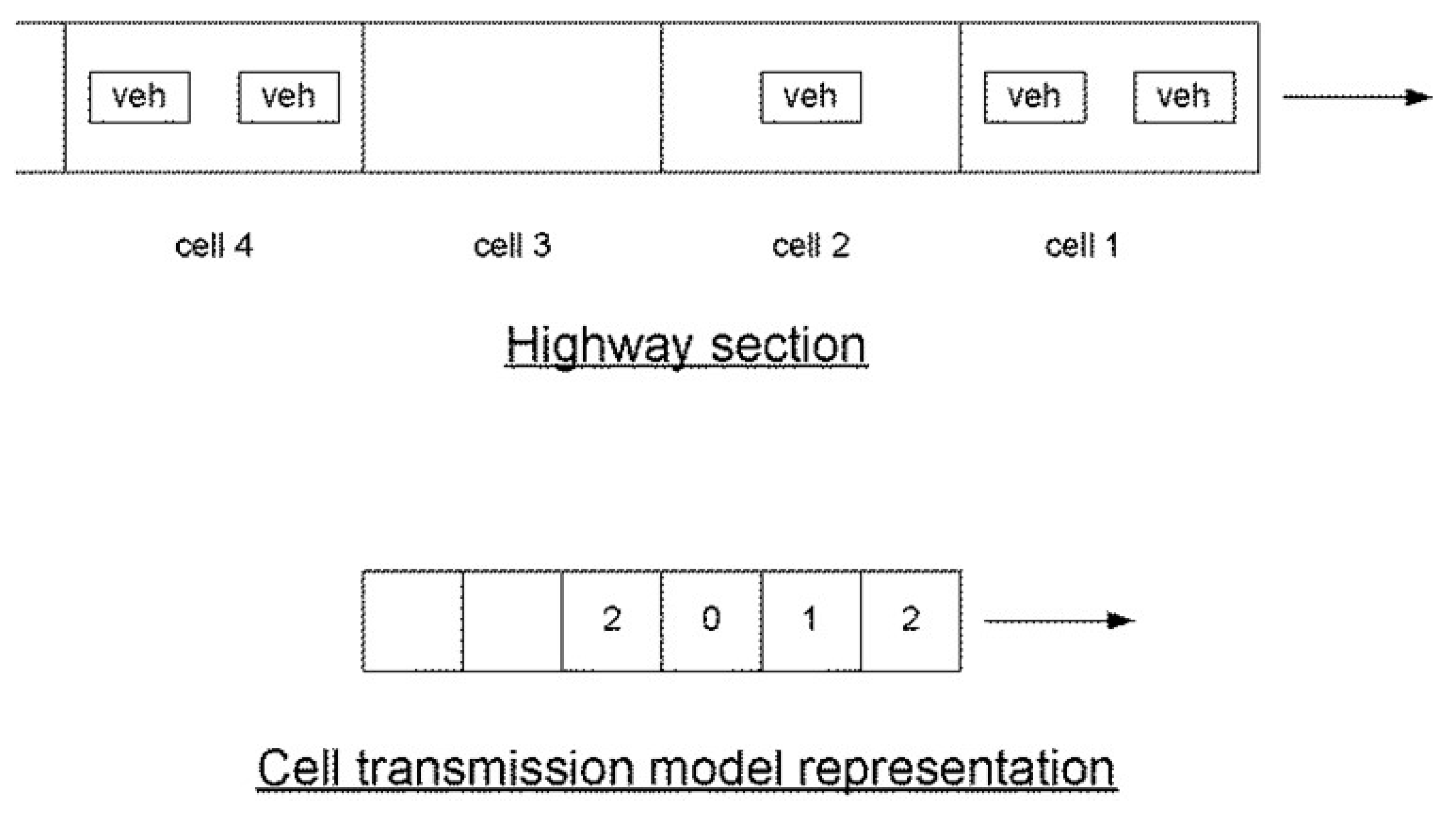
To effectively model the spatial queue dynamics, a CTM was developed to divide a single road link (a group of lanes) into series of unit cells with user-specified holding capacities. By updating the cell occupancies in discrete time steps, this CTM can be used to predict vehicle movements, queue development, and even spillback of physical vehicle queues, as shown in Figure 1. Moreover, a signalized CTM that controls the exit flow variations in signal cells (full saturation flow rate during green signal phase or zero exit flow rate during red signal phase for the signal cells) to optimize traffic signal settings for minimizing the total delay in the entire CTM system based on the scheduled demand inputs was developed. Based on the hydrodynamic theory of traffic flow, the macroscopic Lighthill–Whitham–Richards (LWR) model was formulated by incorporating the continuity (or conservation) equation as a partial differential equation and the fundamental flow–density relationship [23,24]. Daganzo [25,26] formulated the CTM for the LWR continuum model by using a trapezoidal or triangular fundamental diagram. In this CTM, a road lane was divided into multiple homogeneous sections or cells, and the time horizon was partitioned into discrete intervals or time steps. The traffic flow transmitted from an upstream cell to another downstream cell was prescribed based on the associated receiving and sending functions in terms of the free-flow speed, inflow capacity, jam density, and speed of backward shockwave. Again, Figure 1 shows the CTM of queue dynamics, which was adopted in [27,28]. The concepts of merge and diverge cells were introduced in the CTM to replicate traffic movements through a junction. Based on these movements, a road network was constructed and represented with a series of cells, and network traffic with multiple origin–destination (OD) pairs was modeled [27]. Lo [28,29] developed a mathematical programming approach to obtain a signalized CTM by introducing mathematical constraints for traffic signal controls, in which the exit flow capacity of a signal cell was controlled based on signal settings. Effective green durations were the key decision variables for network delay optimization. A dynamic intersection signal control optimization model based on the CTM was developed and applied to practical designs [30]. The latest application of the CTM can be found in [31] for a multi-objective optimization problem considering total delay minimization, throughput maximization, safety, and queue blocking back upstream intersections and lanes. Carey et al. [32] extended the CTM to model lane changes by permitting traffic to move not only along its original inflow lane but also in adjacent lanes. Bottleneck traffic patterns were simulated, and lane capacity reduction due to lane-changing activities was considered [33].
Total delay (and vehicle queuing) minimization using traditional stage- or group- (or phase-) based methods is a nonlinear but “convex” mathematical programming problem, with lane markings and lane flows being fixed as the parameters input by users. However, the lane-based method relaxes the lane markings as binary variables in the design optimization framework, and the associated lane flows, instead of being fixed parameters, become continuous variables in the optimization framework. This minor change simply alters the nature of the problem to nonlinear and “non-convex” for total delay minimization. The non-convexity can be verified by checking the Hessian matrix, which contains the second partial derivatives of the delay with respect to all the traffic signal timings and lane flow variables. The lane-based total delay minimization problem becomes a “non-convex” type binary mixed integer nonlinear programming problem. Piecewise linearization and exhaustive line search techniques, which work well for convex problems, are ineffective and inefficient for solving this non-convex problem. For solving such high-dimensional nonlinear non-convex mathematical programming, a cutting plane method could be applied, in which a series of linear hyper planes is added until a sufficient number of linear planes is created to replicate the original nonlinear spherical shape of the solution space. The greater the number of hyper planes added, the better is the solution resolution and quality. The gap between the original total delay and the approximated total delay under the optimized settings was established as the indicator for achieving certain stopping criteria. A few new reliable stopping criteria were established to terminate the solution process (continued addition of hyper planes during the solution process) based on the solution point densities with respect to number of hyper planes being added to the formulation [17]. To terminate the solution process effectively, the solution quality should attain a certain acceptance gap between the true total delay and the approximated total delay at the optimized solution point. To integrate the requirements of the solution gap and the solution density, a two-dimensional stopping criterion was used to accelerate the solution process by relaxing the solution convergence.
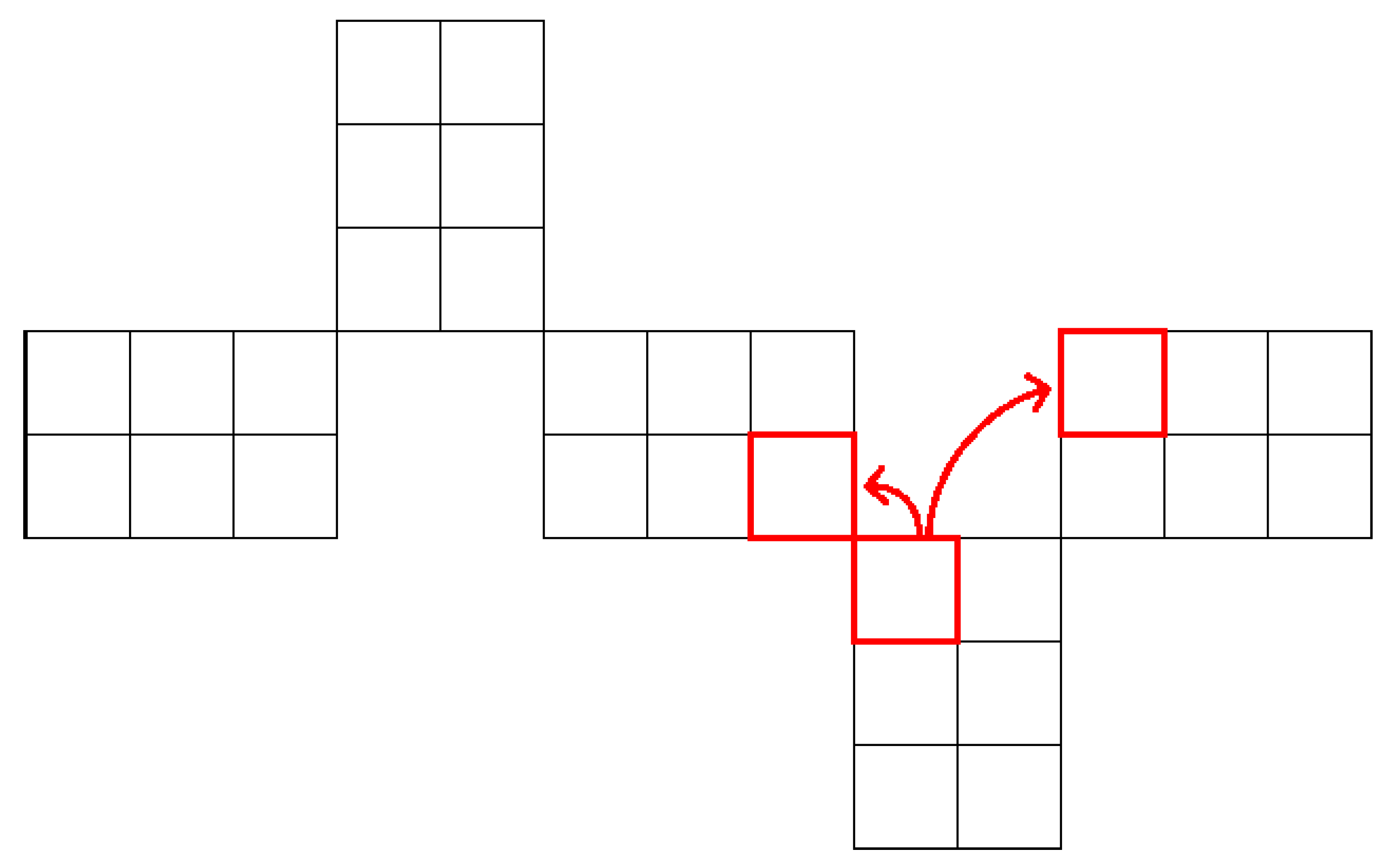
By integrating the lane-based design method with the signalized CTM, a very attractive and direct extension is obtained for utilizing all approach lanes to balance lane flow distributions and utilizations of individual lanes while fulfilling the spatial lane-holding capacities and controlling vehicle queuing to avoid spillback. Wong et al. [34] applied the signalized CTM to model a real intersection with shared lane markings permitting simultaneous left and right turns on nearside approach lanes. In general, the CTM permits different turning directions for signal cells at intersections, and the inflow into the first cell on a downstream link may originate from numerous upstream links through the corresponding sent flow variables. The proportions of sent flows from the ends of all the upstream links into a single downstream link should be specified. Difficulties in practical modeling emerge if the proportion of sent flow in the CTM (or the equivalent lane turning proportion in the lane-based model) is a model variable instead of a fixed user input. Sent flow itself is a model variable that should be equal to the assigned lane flow in the lane-based framework. Figure 2 shows cell representation of a shared lane with simultaneous left- and right-turn movements [34]. To model the shared lane markings in the solution process, the lane turning proportion must be a model variable because it depends on the lane marking patterns and the assigned lane turning flows. To merge these lane-based model parameters into the CTM platform, nonlinearity is induced to help solve a difficult mathematical problem.
Liu and Chang [35] reported that adjacent lane groups could easily be blocked when the corresponding lane markings and shared lane markings are not carefully chosen, especially for the approach lanes with (short) flare lanes under oversaturated conditions. Lu and Yang [36] estimated the dynamic queue distribution in a signalized network by adopting a probability-generating model that modeled queue formation and dissipation, platoon dispersion, queue merging and diverging, queue spillover, and downstream blockage as stochastic events. Liu and Wong [37] developed a heuristic solution algorithm to refine the traffic signal settings for the lane-based model outputs to avoid lane overflow and blockage of back upstream lanes. Excess green durations from non-overflow lanes were shifted as extra green durations to control overflowing lanes. Such a redistribution of green durations by following a manual iterative process is inefficient.
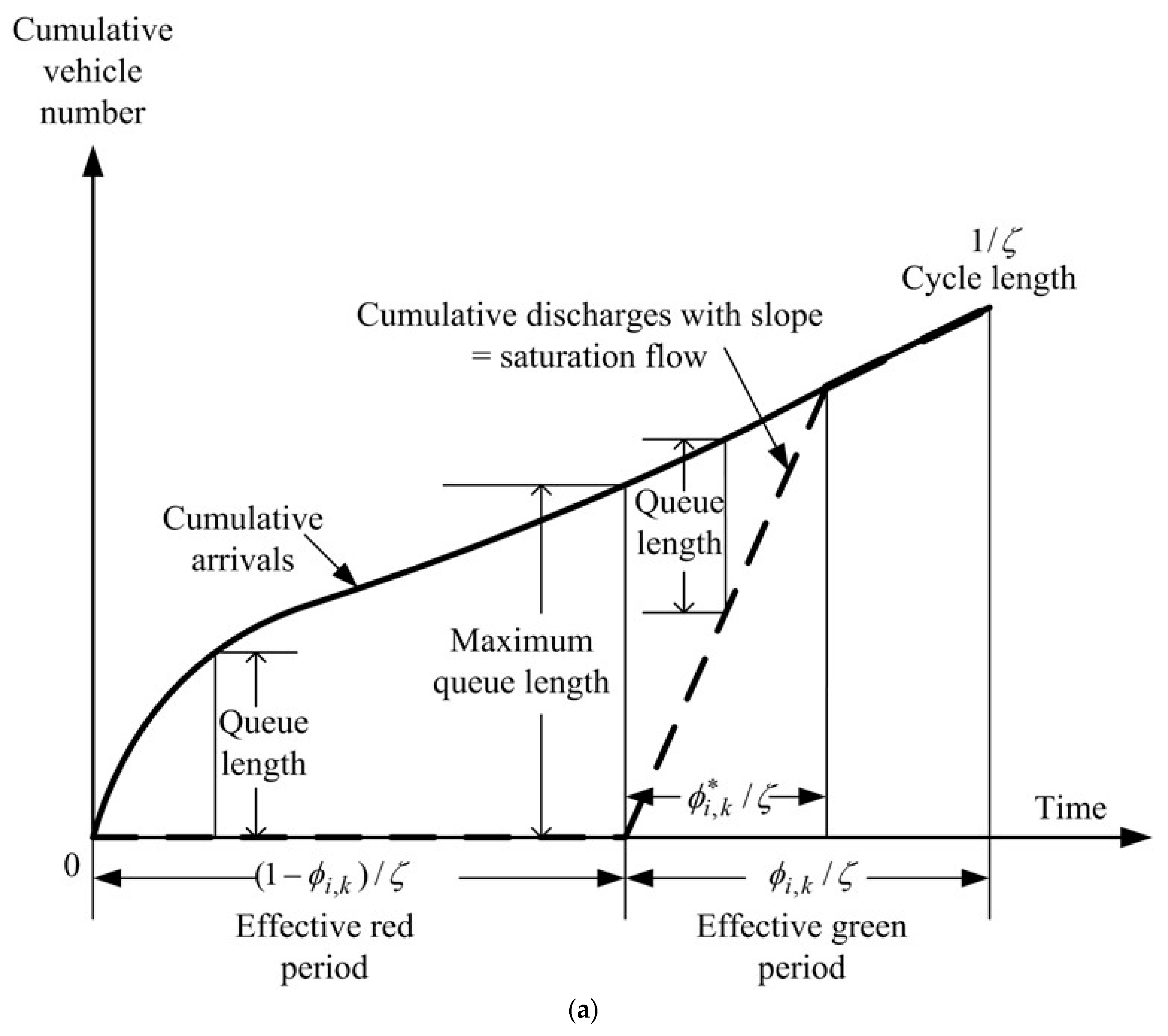
In the present study, we try to enhance the existing lane-based method for designing intersections with short approach lanes that have limited spatial holding capacities. New linear constraint sets are developed to control the effective red and green durations to ensure that waiting queues are not accumulated continuously until overflow but are discharged more frequently by employing shorter cycle lengths with well-balanced effective green and red durations. A case study involving a four-arm intersection with complex movement turns and short lanes is described to demonstrate the defects in the existing (observed) traffic signal settings and optimize these traffic signal settings by using the proposed algorithms. The TRANSYT 15 software is used to simulate the queue dynamics under the optimized traffic signal settings to verify the proposed model. Figure 3a presents the general vehicle queue development along an ordinary approach lane k from arm i [37].
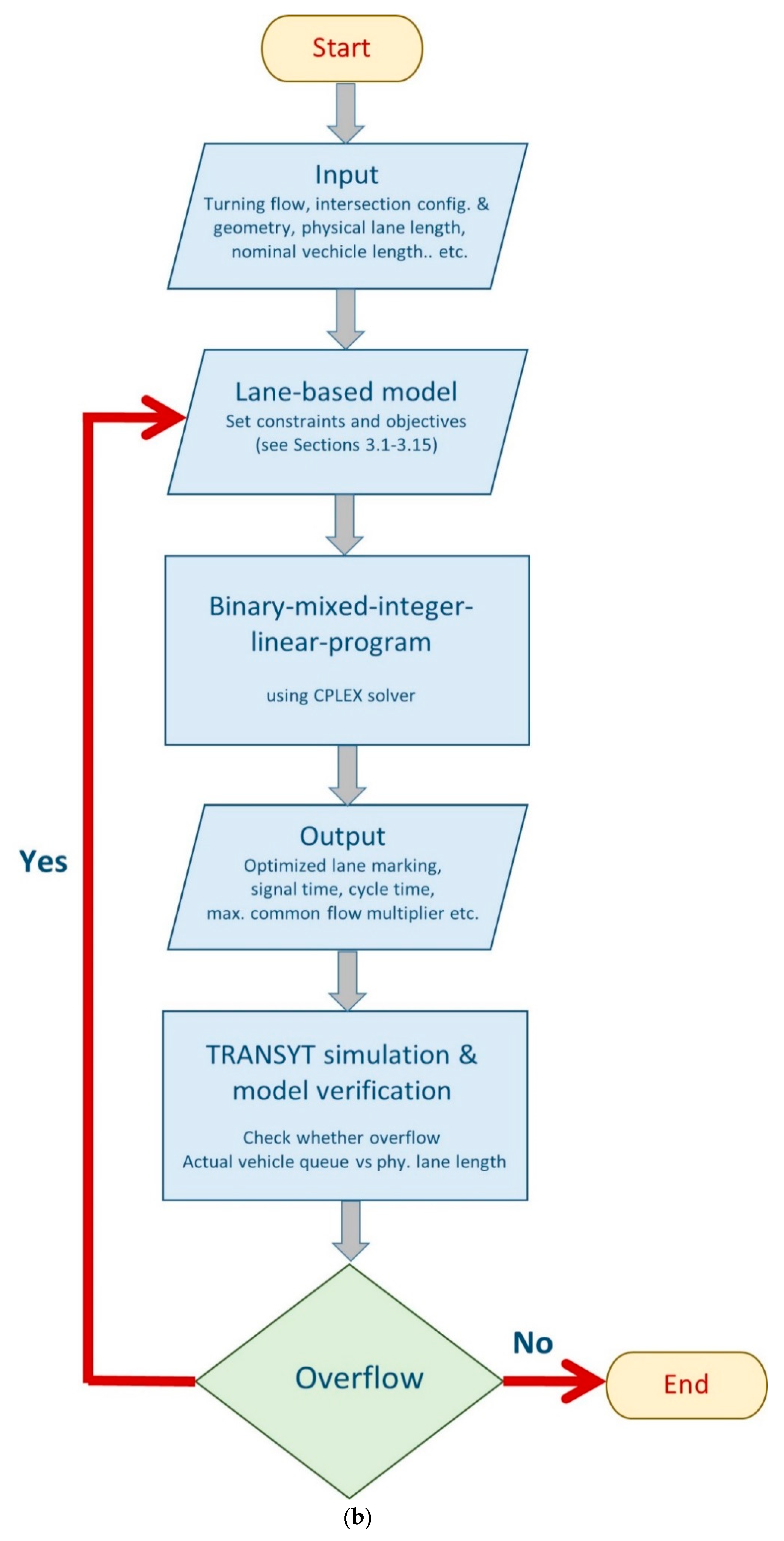
Vehicle arrivals are normally accumulated during the effective red period (i.e., cycle length—effective green period) and held along the road lanes. If the road lanes are physically long enough to hold all the arrivals during the effective red period, there will be no overflow. The maximum queue length is developed at the end of the red time (1 − φi,k) (or just before the start of green time), and the maximum queue length will start to dissolve once the green signal duration commences. If a sufficient effective green duration is designed, the entire queue (length) will be discharged, and no residual queue will be carried over to the next signal cycle. Assuming that the traffic demand enters the approach lane continuously even during the green signal period, the desirable green time φ*i,k should ensure that there is no residual queue in the ideal situation. The duration φ*i,k can be obtained by setting the equality constraint , where φi,k is the green start time, ri,k(τ) is the user-specified function of the traffic demand pattern, and si,k(τ) is the saturation flow rate for approach lane k from arm i. The purpose of the present study is to develop a mathematical model to optimize the traffic signal settings and lane usage in terms of lane marking patterns to control spatial queue developments. We must therefore estimate the physical holding capacities of the approach road lanes for further analysis. Let li,k be the actual length of the approach road lane k from arm i (in meters), and let Lv be the physical length of a standard vehicle v plus a nominal length gap between the front and rear bumpers of two consecutive vehicles occupying the road space (in meters/pcu). The lane-holding capacity can then be defined as li,k/Lv, which represents the maximum number of standard vehicles that can be held up and occupy the approaching traffic lane (in pcu). Figure 3b shows the flowchart of solving this lane-based problem, which consists of parameter input, optimization output, binary-mixed-integer-linear-program and TRANSYT modelling/simulation. One of the contributions in this paper is to develop a new optimization module to optimize the traffic signal settings including red duration, green duration, cycle times and lane markings altogether in a unified platform. New linear constraint sets have been developed to control the red duration, green duration, and cycle times, which are compatible to the original lane-based model constraint sets. It was already proven by Liu and Wong [37] that the cycle time must be reduced to let through traffic more frequently along short lanes for preventing long vehicle queues. There was one drawback in [37]. The solution resolution was set to be 1 s while reducing the cycle time length sequentially until overflow queues were eliminated. The whole solution process had to be implemented manually through the steps in the flowchart. In this paper, the enhancement is a robust formulation to optimize all of the key model variables simultaneously and to minimize the solution resolution as fine as possible (decimal place accuracy). The proposed TRANSYT model can show the vehicle queues along all lanes within a typical signal cycle while operating with optimized traffic signal settings and optimized lane markings.
3. Lane-Based Optimization for Traffic Signal Settings with Controls in Effective Red Duration Times
3.1. Maximum Effective Red Duration to Avoid Traffic Overflowing
Referring to Figure 3a, vehicle queues are developed during the effective red period. Longer vehicle queues are held along the road lanes if longer effective red times are displayed. Ideally, a maximum effective red duration time (in seconds) should be set for lane k from arm i to control the maximum queue length along the road lane as in Equation (1). Note that all notations and their definitions are shown in Appendix A.
In this formulation, the lane flow qi,j,k is a set of continuous model variables that depend on the lane marking patterns (binary variables). is a set of continuous variables that depends on another set of total lane flow variables and the actual lane-holding capacity li,k/Lv (in pcu). Direct multiplication of these two continuous variables would turn Equation (1) into a nonlinear equation.
With the computed using Equation (1), is defined as the associated effective red duration for a fraction of a signal cycle (=/cycle time or ). is the cycle length given by the reciprocal of the actual cycle time. As the cycle time or cycle length is defined as a continuous model variable, Equation (2) is also a nonlinear equation.
Directly including Equations (1) and (2) in the lane-based optimization framework induces nonlinearity, which makes solution process difficult. Thus, Equations (3)–(5) are developed to replace Equations (1) and (2) to model the required solution space. The idea is as follows. For example, if the total lane flow for all movement turns in the approach lane k is 360 pcu/h, which is equivalent to 0.1 pcu/s (assuming an uniform flow arrival pattern), and the lane-holding capacity is 10 pcu, the maximum red time can be up to 100 s for the incoming demand vehicles to queue up horizontally without overflowing. If the cycle time is 120 s, the corresponding is 100/120 = 0.8333. To model these solution conditions in a linear framework, we must develop a series of linear constraint sets in Equations (3)–(5).
where H is defined as the total number of discrete segments to discretize the maximum cycle time . For example, if = 120 s with 1 s model resolution for each segment, H is equal to 120 segments. To increase the solution resolution by using smaller segments, such as 0.5-s segments, H should be increased to 240 segments. To this end, more constraint sets are required. Thus, h − 1 is the number of segments required to model the effective green duration. in Equation (3) becomes a constant input by the user. Based on the concept of Equation (1), we can calculate all as exogenous inputs in Equation (3). The value of h should numerically range from 1 to H. is a binary variable indicating whether lane k from arm i is overflowing ( = 1) when the effective green duration is h − 1 segments.
Based on users’ exogenous inputs , Equations (1) and (2) can be applied again to calculate as another set of exogenous inputs for Equations (4) and (5).
Whenever both σh,i,k and σh+1,i,k are zero, especially for the case of h = 1, Equation (4) can be used to assign the longest available effective red duration to the variable , which implies that the assigned lane flow in the approach lane k is very small, and the cumulative queue length will not lead to overflow, even when the longest red duration is assigned.
Similarly, the solution process checks all approach lanes for their assigned lane flow intensities to ensure that the maximum effective red times are derived without triggering the overflow conditions. Equation (5) continues to search within the traffic signal cycle in all discretized time segments till the end at H − 1.
To effectively merge the effective red time requirements as restricted by the linear constraint sets in Equations (3)–(5), Equation (6) is developed as the key interface to link it with the existing lane-based optimization framework. Within a signal cycle, the cycle time should be the sum of the effective green and red durations. In the proposed lane-based optimization framework, 1 − (φi,k + e) represents the effective red duration, which should always be less than the maximum effective red duration, as required in Equation (6), where e is the time difference between the effective green and actual display green durations.
Equation (7) is required to ensure that the designed minimum effective red duration is always longer than the user-specified minimum red duration as a basic safety requirement.
3.2. Input Demand Flow Conservation
Considering the definitions in [22],
where Qi,j is the users’ input demand flow for movement turns from arm i to arm j, Ki is the total number of approach lanes from arm i, and is the total number of arms at the intersection. Equation (8) is the flow conservation equation for controlling the assigned lane flows to match the demand flow patterns.
3.3. Minimum Lane Marking on Approach Lanes
Equation (9) is used to control the binary lane marking variable to ensure that at least one lane marking is optimized for each approach lane k. All approach traffic lanes should be utilized to serve the assigned lane flows [38].
3.4. Maximum Lane Marking for Exit
Equation (10) is used to prevent the total number of lane markings for a turn at an upstream junction from exceeding the total number of exit lanes to enter the downstream lanes to avoid unnecessary traffic merging.
where is a user-defined function for identifying the downstream traffic arm receiving traffic from the upstream intersection turning from arm i to arm j, and is the total number of exit lanes available at the downstream lanes to receive the turning traffic.
3.5. Compatible Lane Markings Across Adjacent Approach Lanes
Equations (11) and (12) are used to avoid any likely internal clash of traffic within the same arm for different movement turns [38]. Practically, left-turn traffic should not be assigned to right-hand lanes because the left-turn traffic movement could possibly clash with the right-turn or straight-ahead traffic movements if the latter are assigned to some left-hand lanes. In an arm, traffic turnings should be controlled, and their effective green durations should be well arranged to separate their rights-of-way. Thus, the lane markings on adjacent lanes within an arm should be governed using Equations (11) and (12).
where the function represents a left-turn movement, represents a straight-ahead movement, and represents a right-turn movement for traffic turning from arm i to arm j at the intersection.
3.6. Operating Range of Cycle Length
Equation (13) is developed to provide a suitable operating range of the cycle length (reciprocal of cycle time c). Users may specify the minimum bound and the maximum bound for optimizing the operating cycle length [38].
3.7. Synchronization of Traffic Signal Settings for Approach Lanes and Movement Turns
Equations (14) and (15) are required to ensure that the signal timing display patterns, including the starts and durations of the green times, are consistent across approach lanes and movement turns. The lane marking variables state the actual lane usages. The traffic signals for controlling the traffic turns must be identical to the movement turns in the lanes [38].
3.8. Start of Green Durations within the Signal Cycle
Equation (16) is used to provide a suitable solution range for the start of green duration variables. In the present formulation, traffic signal timings are repeated cyclically. Thus, the green start times must be optimized within a signal cycle [38].
3.9. Maximum and Minimum Ranges of Green Durations
Equation (17) ensures that the maximum green duration is one signal cycle, and the minimum green duration is longer than the user-specified minimum green time [38].
3.10. Regulating the Order of Conflicting Traffic Signal Settings
Equation (18) ensures that any pair of conflicting movements, including vehicular (traffic from different arms) and pedestrian phases, are ordered sequentially to receive the right-of-way in a signal cycle [38].
where Ψs is a set of conflicting movements at the intersection, as defined by users.
3.11. Minimum Clearance Time to Separate Conflicting Movements
Equation (19) provides adequate clearance (or inter-green) time to separate the rights-of-way of conflicting traffic movements in the traffic signal settings [38].
where M is an arbitrary large positive constant number, and is a user-specified minimum clearance time for a pair of conflicting traffic movements .
3.12. Eliminating Redundant Lane Markings
Equations (20) and (21) prevent one from designing lane markings for traffic movements with zero demand flows [38].
3.13. Identical Flow Factors Across Adjacent Lanes with Identical Lane Markings
Equation (22) forces the flow factors for a pair of adjacent lanes to be identical if identical lane markings are designed [38].
where and are the constant lane saturation flows for straight-ahead movements on approach lanes k and k + 1, respectively.
3.14. Restricting the Maximum Acceptable Degree of Saturation
Equation (23) is used to evaluate the degree of saturation for approach lanes. As a safety factor, a user-specified maximum flow-to-capacity ratio is set as the maximum limit.
where (=90%) is the maximum degree of saturation on lane k from arm i at the intersection, and e is the difference between the actual and effective green times (usually taken as 1 s).
3.15. Objective Function by Maximizing Common Flow Multiplier
In the present study, we optimize the traffic signal settings together with the lane marking patterns to strictly control the queue length development without inducing overflow. It is well known that if the optimized common flow multiplier is higher than 1.0 numerically for an intersection, the intersection is considered unsaturated, implying that all incoming traffic can leave the intersection at the end of a signal cycle. If is less than 1.0 in the optimization process, the intersection is considered overloaded. Not all incoming traffic can leave the intersection at the end of a signal cycle, and a residual queue exists. These residual queues occupy space and reduce the holding capacity of road lanes. Thus, overflow can occur more easily. Maximizing the common flow multiplier to maintain an unsaturated condition leads to a stable control system. Moreover, when formulating the optimization problem in a linear optimization framework, the standard branch and bound method can be used to optimize the global optimum solution. Therefore, it is proposed in the present study to directly optimize the common flow multiplier subject to the linear constraint sets in Equations (3)–(23). The resultant problem becomes a binary mixed integer linear program, which can be solved with a well-known solver based on the simplex method implemented in the C programming language, which is called CPLEX solver.
4. Case Study for Demonstration
4.1. Background
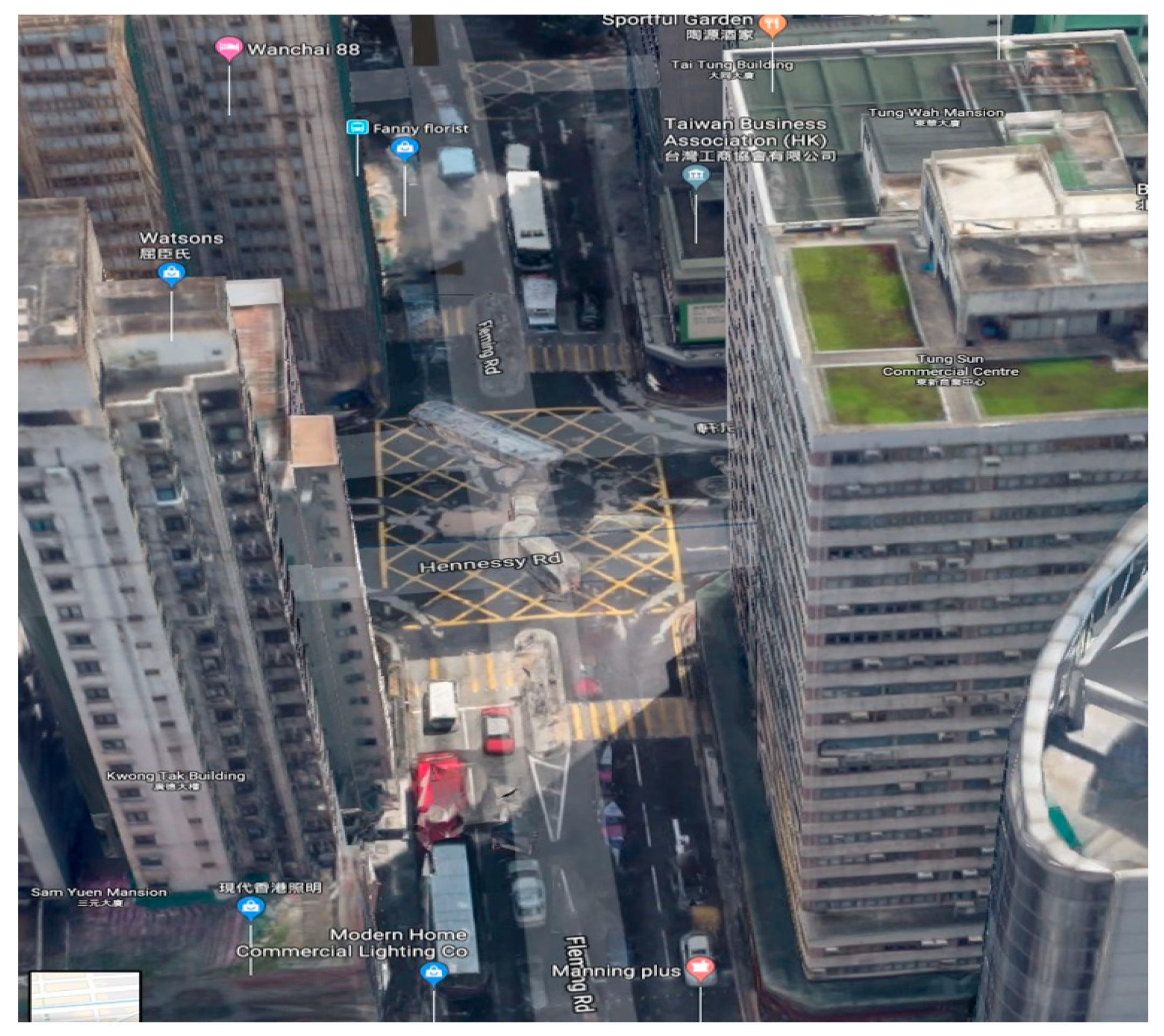
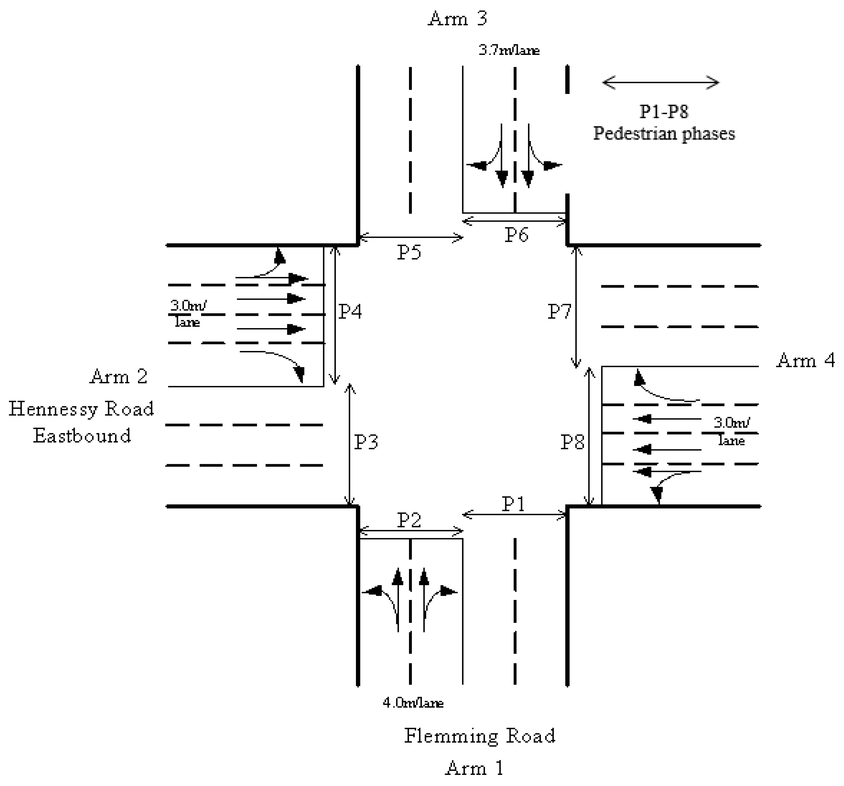
For demonstration, the enhanced lane-based method is used to solve the most complicated signal-controlled intersection on Hong Kong Island. This intersection is located in Wan Chai between Hennessy Road and Fleming Road, as shown in Figure 4. It is a four-arm intersection with left-turn, straight-ahead, and right-turn traffic movements from all arms and pedestrian crossings at the intersection that are perpendicular to all traffic lanes. Figure 5 shows the existing settings of the lane marking patterns and pedestrian crossing arrangements. A manual classified count survey was conducted at the intersection to record turning flow patterns covering the morning-, off-, and evening-peak periods. Table 1 lists all of the observed traffic counts at the study intersection, which was adopted in [20]. The existing traffic signal settings, including green start, duration, and cycle times, were surveyed, and are also listed in Table 1.
Traffic lanes have different widths (i.e., different saturation flows or discharge rates) and lengths with different spatial holding capacities. Hennessy Road is a major road. There are four approach lanes and three exit lanes for both eastbound and westbound traffic. Fleming Road is a minor road with two approach lanes and two exit lanes for both southbound and northbound traffic. The widths of various lanes were recorded at the site, and are presented in Figure 5 to calculate the lane saturation flows. To model the actual spatial holding capacities of all the approach lanes, the physical road lengths (from the intersection to its upstream intersections) were measured. The lane lengths along Hennessy Road = 90 m for Arms 2 and 4, and the lane lengths along Fleming Road = 30 m for Arms 1 and 3. We assume the standard vehicle length for 1 pcu is 5 m and there exists a 1 m safety gap between consecutive pairs of vehicles. Thus, = 6 m is set. The spatial holding capacity of the approach lanes from Arms 1 and 3 are 5 pcu and that of the approach lanes from Arms 2 and 4 are 15 pcu. Therefore, the approach lanes from Arms 1 and 3 are short lanes and expected to overflow easily depending on the incoming traffic intensities. The turning radii of all of the left- and right-turn movements from all approach lanes are assumed to be 12 m, and this value is used to revise the lane saturation flows whenever turning traffic existed in the approach lanes. The minimum green and clearance (inter-green) times to separate conflicting movements are all set to be 6 s. According to the observed traffic patterns and traffic signal settings, the intersection capacities across all the peak periods are with positive reserve capacities (RC), implying that no residual queue should exist at the end of a signal cycle at the intersection.
Based on Equation (1) with the inputs mentioned above, the maximum effective red durations are = 54.40 s and = 50.98 s for the nearside and non-nearside lanes, respectively, in the morning-peak period. The observed effective red duration for both the nearside and non-nearside lanes is 81.0 s (=105 – 23 − 1, as given in Table 1). This simply implies that although the R.C. is positive in the morning-peak period, the approach lanes from Arm 1 overflowed. Indeed, all of the short approach lanes from Arms i = 1 and 3 overflow in all study periods. Therefore, we apply the same intersection settings for optimization using the proposed algorithms to avoid the overflow condition. The relevant optimization results are presented in Section 4.2.
4.2. Optimization Results Using the Proposed Optimization Algorithms
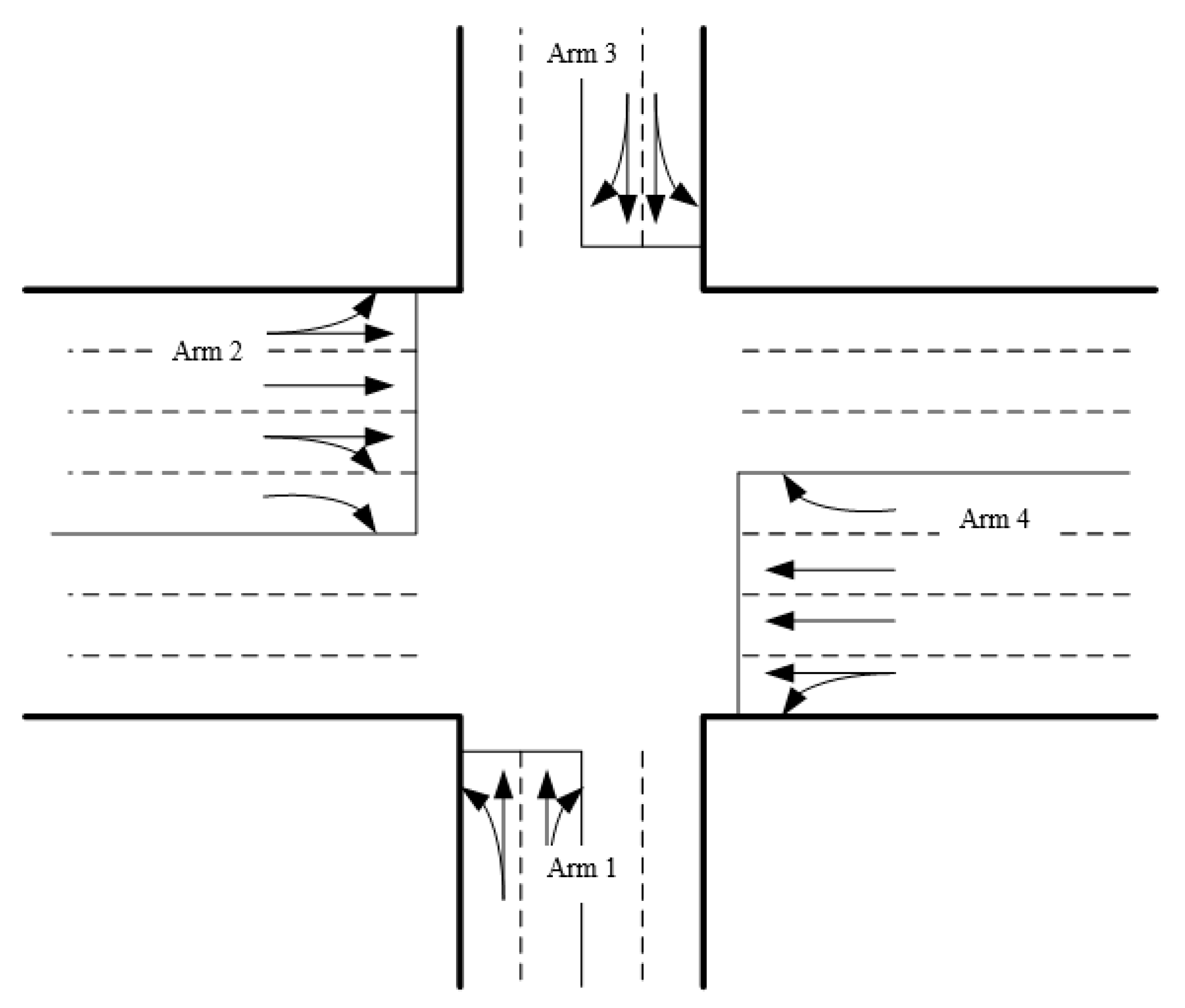
Having introduced the background of the study intersection, we find that the observed traffic signal settings are unreliable in practical operation. Overflow can occur along the short approach lanes from Arms i = 1 and 3. To avoid this, we apply the proposed optimization algorithm for this study intersection to examine its effectiveness in tackling the lane overflow problem. We maximize the common flow multiplier subject to the linear constraint sets in Equations (3)–(23). Details of the modeling results are given in Table 2, Table 3 and Table 4 for the morning-, off-, and evening-peak periods, respectively. The optimized lane marking patterns are shown in Figure 6 [37]. One additional right-turn lane marking is added to approach lane k = 3 from Arm i = 2 to the existing design. Lane markings on the short lanes from Arms I = 1 and 3 have no changes. Table 2, Table 3 and Table 4 list the optimization results for the traffic signal settings in various study periods, including lane traffic flows, turning proportions, flow factors, starts and durations of green times, and maximum spatial queue lengths. The maximum queue lengths along the approaching traffic lanes from Arms 1 and 3 are lower than their respective spatial holding capacities. These results prove that the optimized traffic signal settings are superior and more reliable for practical operations.
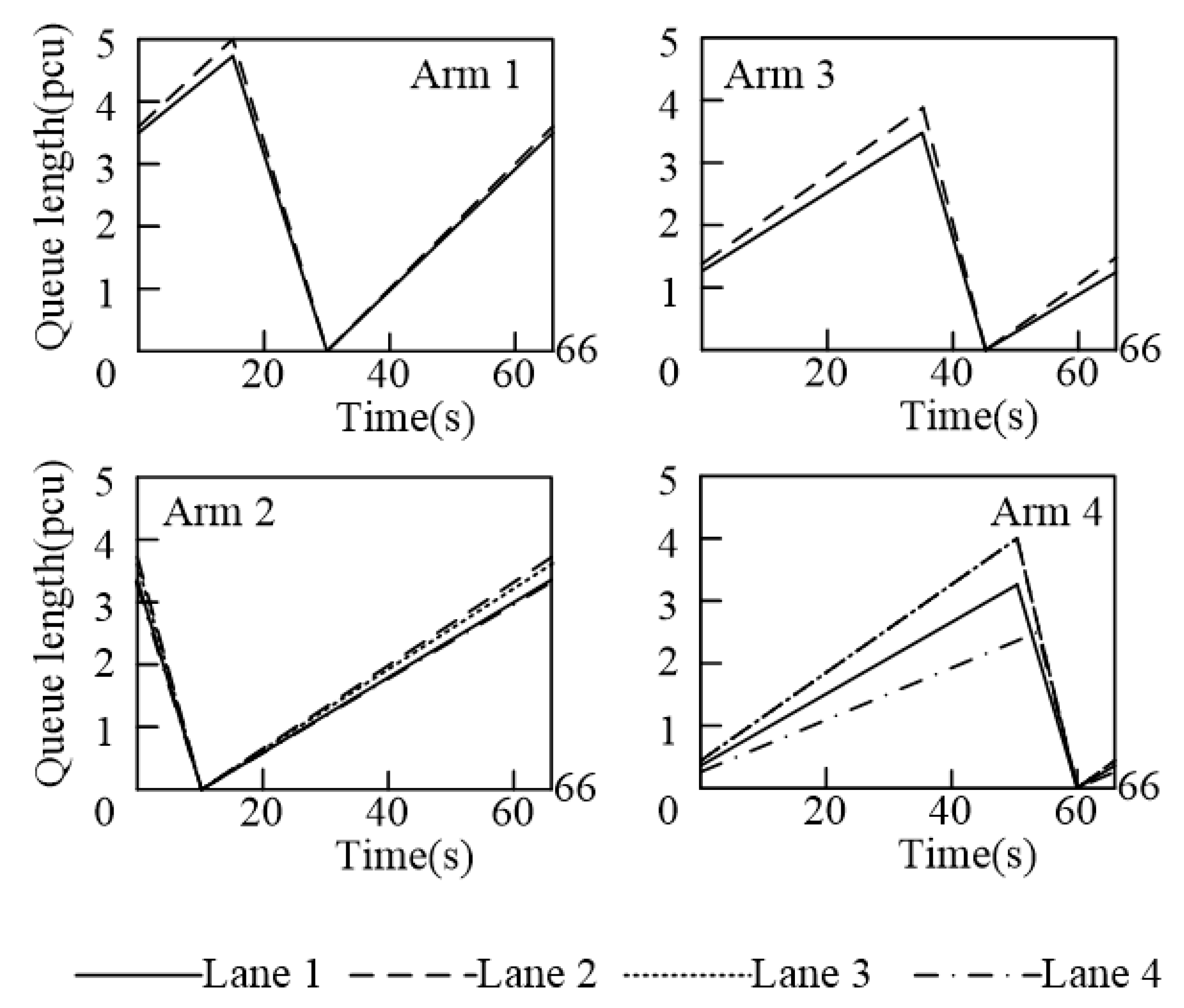
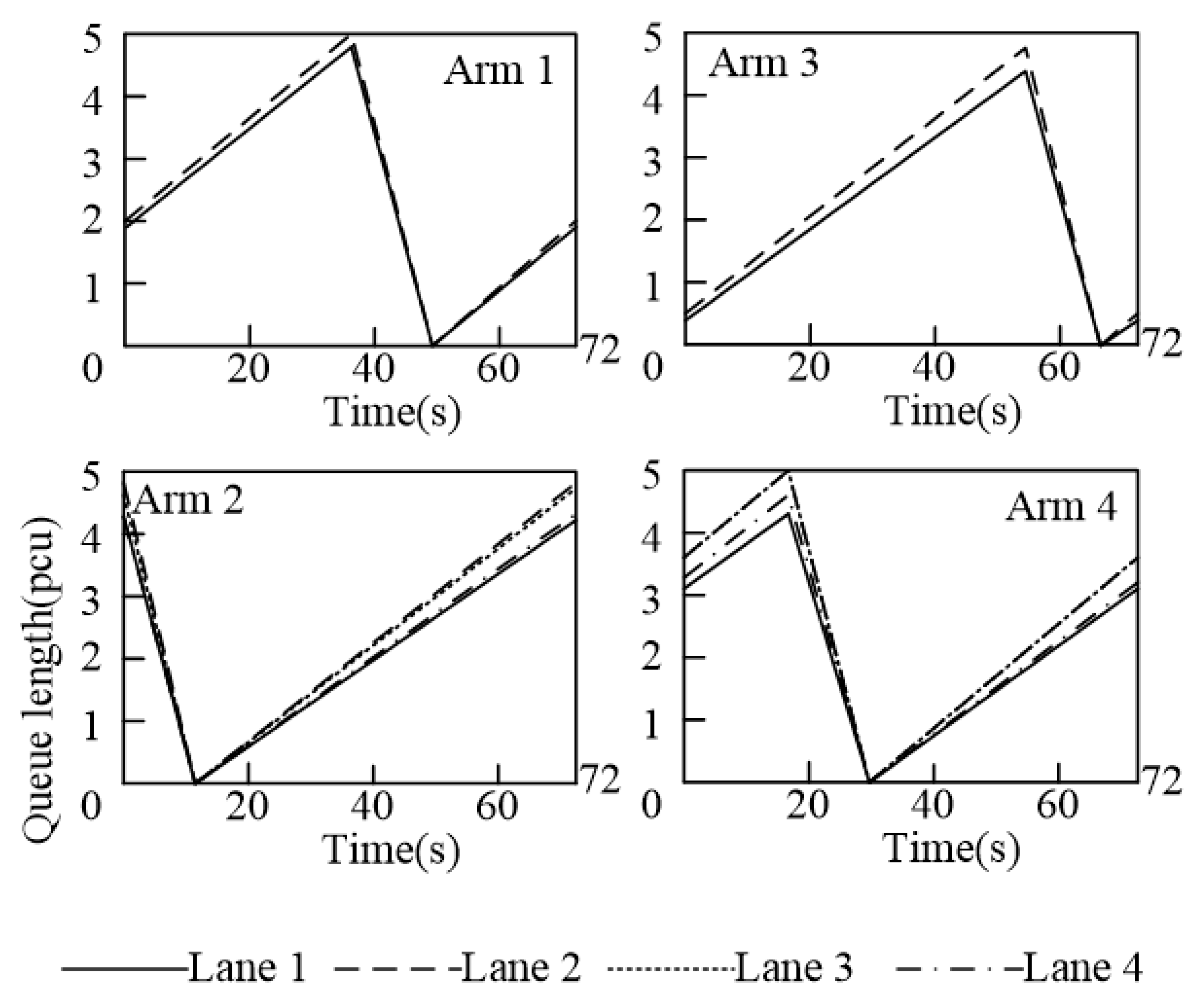
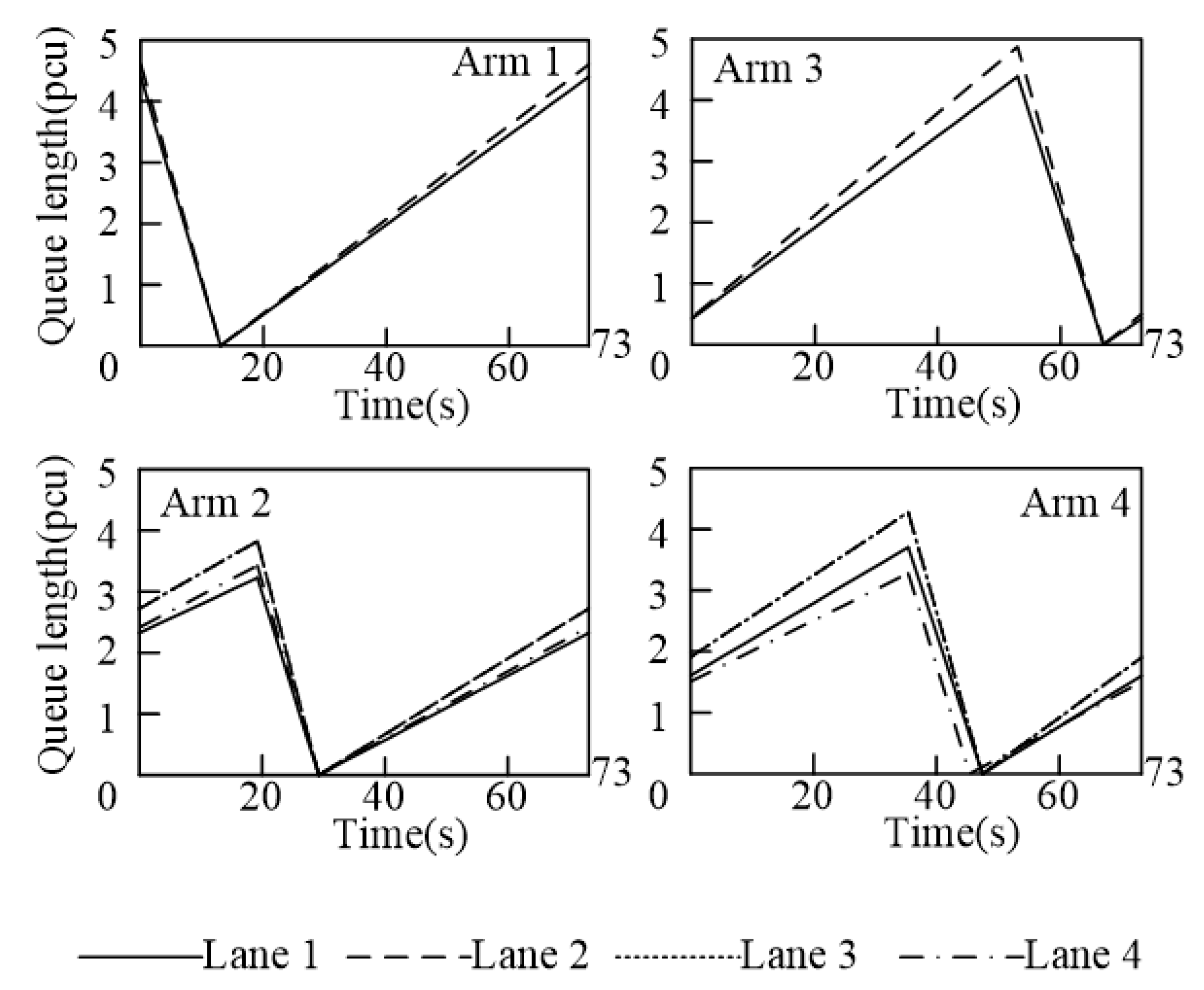
To examine the effectiveness of the optimized signal timings with very different green durations and cycle times from the optimization results in Table 2, Table 3 and Table 4, the vehicle queuing patterns are plotted in Figure 7, Figure 8 and Figure 9 for the morning-, off-, and evening-peak periods, respectively. The vertical axis represents the queue length in pcu, and the horizontal axis represents the time in seconds. As the corresponding common flow multipliers are all positive, no residual queues are left for the next cycle. The short lanes are from Arms i = 1 and 3 with relatively small spatial holding capacities of 5.0 pcu. The approach lanes from these critical arms can hold their maximum queues without exceeding their respective lane-holding capacities. The optimized traffic signal settings can control the incoming traffic without overflowing and blocking back upstream lanes.
4.3. Evaluations of Optimization Results Using the TRANSYT 15 Simulation Module
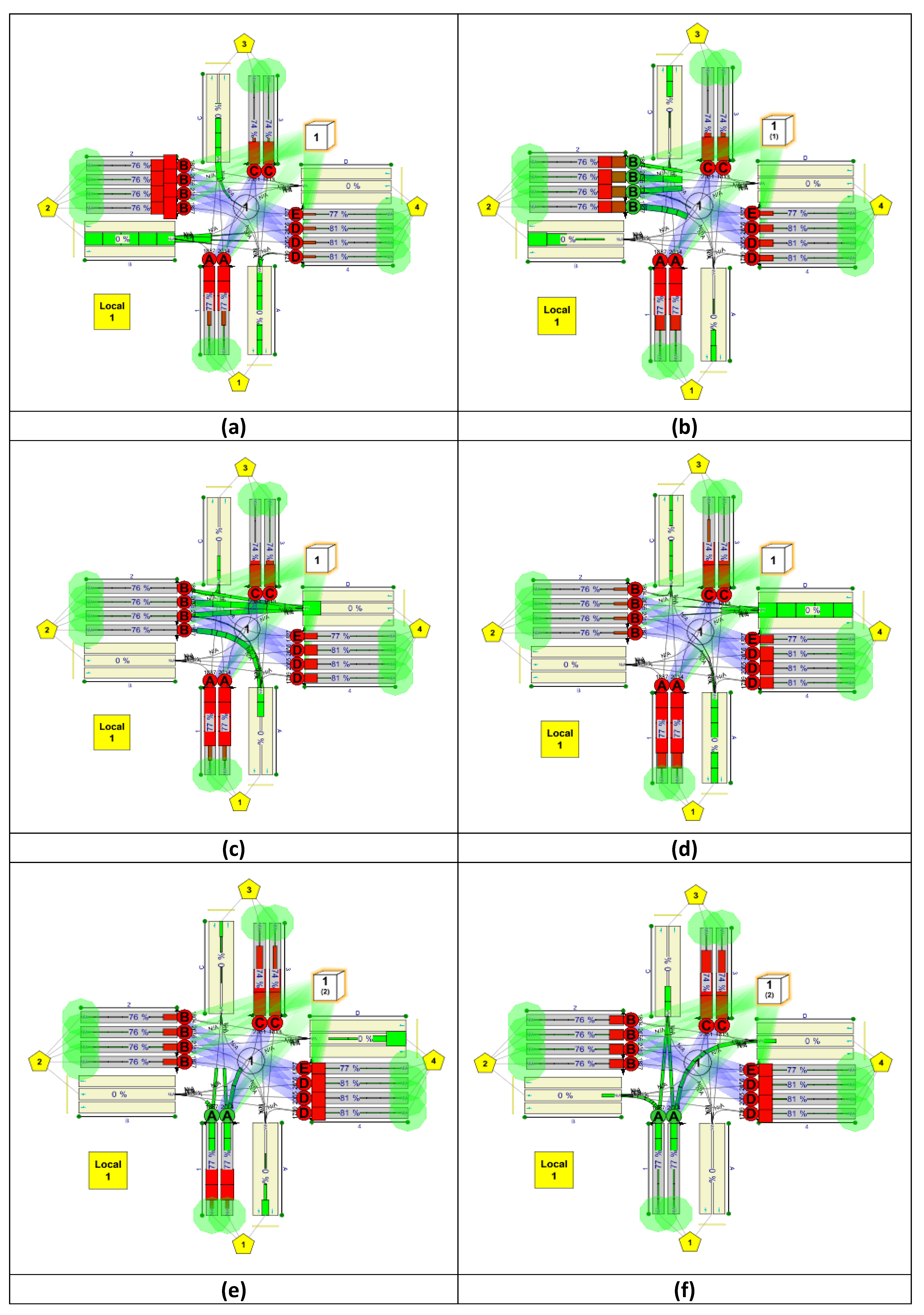
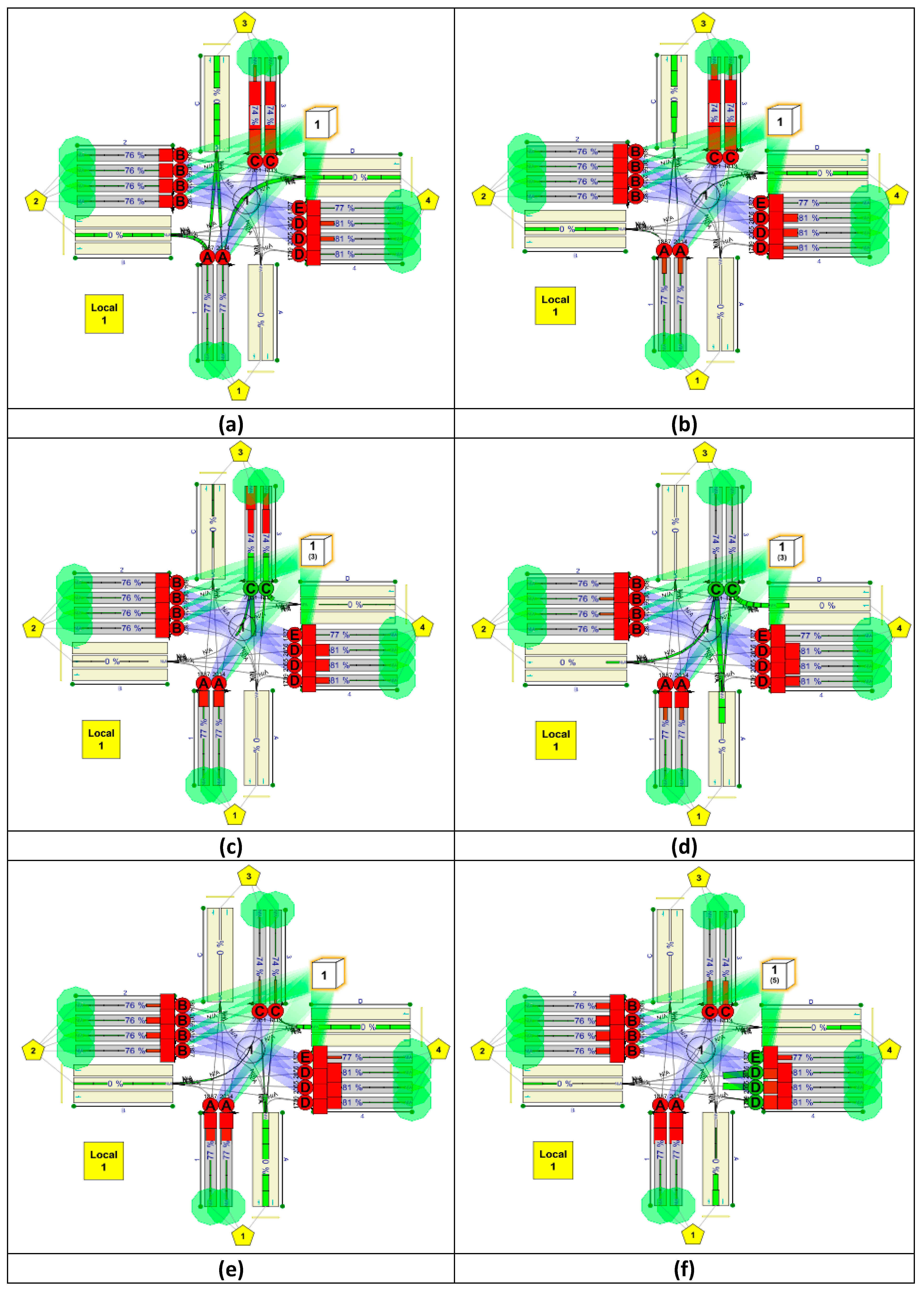
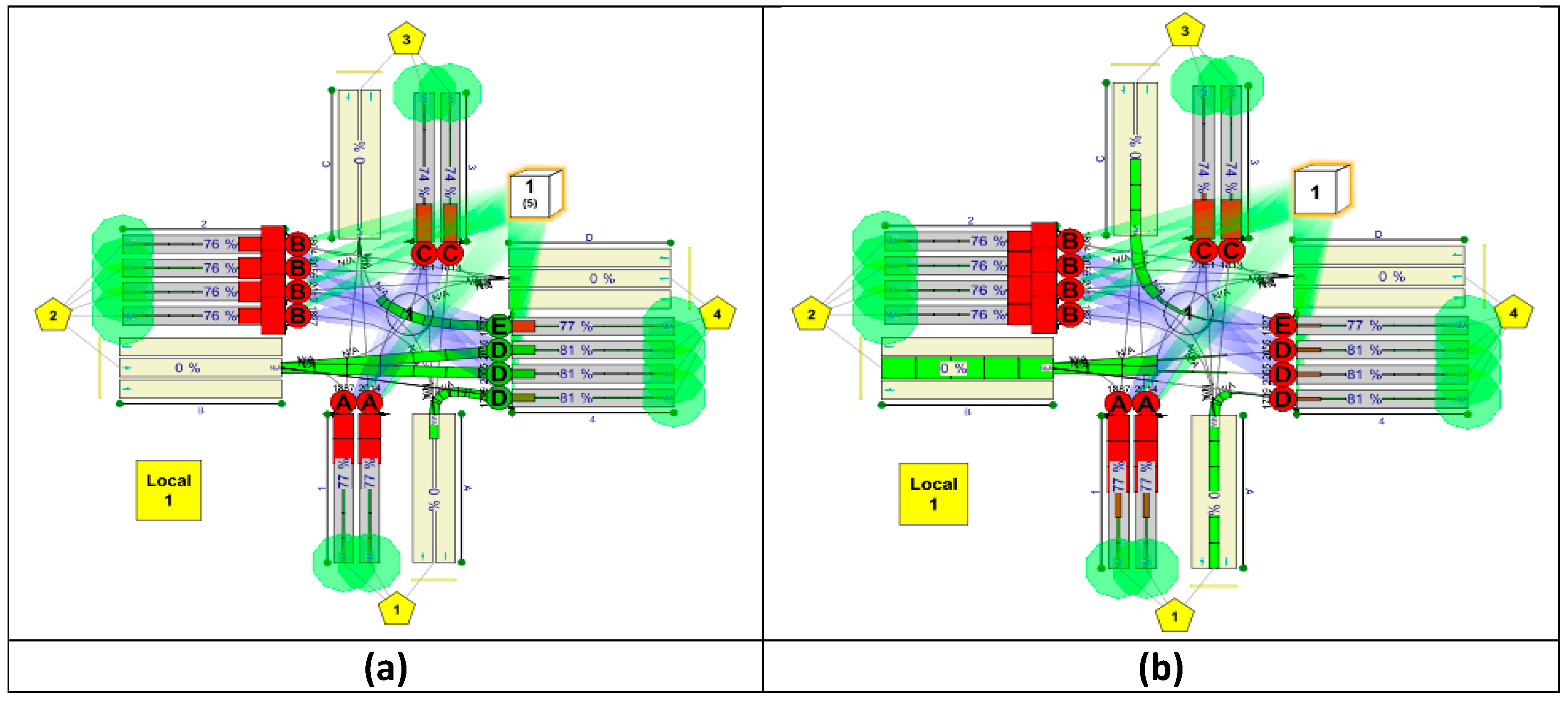
In the case study intersection, the maximum queue lengths are generally longer than the lane-holding capacities in all study periods under control using the observed signal timings. Thus, the approach traffic lanes from Arms i = 1 and 3 overflow. According to the results reported in the previous section, all the maximum queue lengths are within the lane-holding capacities for the entire intersection when the optimized traffic signal settings are implemented. This demonstrates the effectiveness of the proposed enhanced lane-based optimization method that considers the spatial capacities of all the approach traffic lanes. To evaluate the proposed optimization framework, the maximum queue lengths are the key parameters that should be studied. Overflow occurs if the maximum queue lengths are too long for the physical holding capacities of the approach lanes. A TRANSYT 15 simulation is developed to model the case study intersection by taking the enhanced lane-based optimization model results as inputs. The optimized intersection layout is built in the TRANSYT 15 platform, including the approach and exit lane details. According to the optimized lane marking results, the approach lanes should be properly connected to the various exit lanes in the TRANSYT 15 modeling platform. We then prepare the entry flow patterns based on the observed traffic counts listed in Table 1. Then, we add the optimized turning flows to the fixed flow by using the path menu of the OD matrix data. By using the controller stream menu, we can input the traffic signal groupings based on the optimized traffic signal settings, minimum clearance times for incompatible traffic streams, and optimized cycle time. The optimized signal timing sequence for regulating the traffic movement patterns within a signal cycle should be entered in the phase library. In the resulting phase menu, the exact green start and green end times for all phases are input based on the optimized signal settings. In the traffic option menu, the CTM is selected as the traffic model. In the traffic stream menu, the lane saturation flow figures are specified according to the optimization results. Moreover, cruise speed and turning radius are input into the CTM by using the traffic stream flow menu. After these data are input, the CTM is ready to run. After including the relevant optimization results and turning demand flow inputs during the morning-peak period in the CTM, the simulation results and the queue length development details for all approach lanes are captured in Figure 10, Figure 11 and Figure 12 for one typical signal cycle. The red bars along different approach lanes represent the queue lengths for various simulated signal cycles. Notably, all circles are green in the TRANSYT model at the ends of all approach lanes throughout the signal cycle, thus confirming that there is no overflow in all the arms at the intersection. Moreover, the vehicle queue development patterns along different approach lanes in the CTM are consistent with the optimized queuing patterns in Figure 7. For example, along the short lanes from Arm 1, the maximum queue length, which is represented by the longest red bar in Figure 10, Figure 11 and Figure 12, appears at approximately 15 s, and it is consistent with the Arm 1 pattern in Figure 7. If we follow the changing patterns of the green bars in Figure 10, Figure 11 and Figure 12, the flow movement patterns can be traced. The numerical results of the maximum queue lengths obtained using the simulation model are given in the last columns of Table 2, Table 3 and Table 4.
4.4. Application of Proposed Optimization Framework to Manage Residual Queues
We apply the proposed optimization method to maximize the common flow multiplier subject to the governing constraint sets. We find that the RCs in all study periods are positive and the optimized traffic signal settings were effective for controlling the demand traffic without the occurrence of overflow. Another implication of a positive reserve capacity result is that there should be no residual queue at the intersection after each signal cycle. We now apply the proposed optimization model to manage a more difficult condition with a residual queue from the previous signal cycle. Due to the existence of this residual queue, the respective lane-holding capacities should be reduced to change the initial model conditions. It is expected that the optimized traffic signal settings will be changed to dissolve the vehicle queues. By using the proposed algorithm, we can model the existence of the residual queue by reducing the lane-holding capacity from li,k/Lv to li,k/Lv minus residual queue length in Equation (1). Then, will decrease accordingly by . Equations (4) and (5) should be revised accordingly. However, the effective green duration should be identical to that in the previous optimization results, as if the residual queue does not exist. Using an additional equality constraint set, the green duration should be set to be equal to that in the previous optimization result. As a numerical demonstration, we set the residual queue length to 0 (as Application 1), 1 (as Application 2), and 2 (as Application 3) in approach lane k = 1 from arm i = 1 for optimization. With these revised model inputs, the proposed lane-based model could be applied to maximize the common flow multiplier . In Applications 1 and 2, the reduced cycle time (from 73.17 s to 61.0 s) shortens the effective red duration for arm i = 1, thus preventing excess demand flows from entering lane k = 1 and causing overflow in the system. The optimized common flow multiplier is 1.154 > 1.0. No residual queue is found at the end of the signal cycle. However, for the residual queue length of 2, the optimization result gives a common flow multiplier of less than 1.0, implying that the intersection is overloaded with a residual queue under the control of the traffic signal settings, even when the optimized cycle time is further reduced to 55.0 s.
5. Conclusions
In the original lane-based modeling framework, the point-queue approach yields unreliable traffic signal settings, leading to spatial queues longer than the existing lane lengths. Without accounting for the lane-holding capacities, the lane-based method tends to optimize the traffic signal settings in terms of the maximum allowable cycle length. The enhanced lane-based model with new design constraint sets to restrict the effective red, effective green, and cycle durations can prevent traffic overflow that will block the traffic upstream. The proposed constraint sets are fully compatible with the original lane-based optimization framework. By maximizing the common flow multiplier, the design problem is formulated as a binary-mixed-integer linear programming problem that can be solved using the standard CPLEX solver. Several busy and complex signal-controlled intersections in Hong Kong have been selected in the case study. The proposed model is applied to refine the traffic signal settings to eliminate traffic overflow in short lanes. All short lanes are overloaded under the observed traffic signal control plans. The situation is fully repaired using the proposed optimization model. The results are simulated using the TRANSYT 15 package to verify the proposed model. From the results, it is shown that the maximum queue lengths along the approaching traffic lanes are lower than their respective spatial holding capacities. The optimized traffic signal settings are superior and more reliable for practical operations. The optimized traffic signal settings can control the incoming traffic without overflowing and blocking back upstream lanes. Using the proposed additional equality constraint set, the green duration should be set to be equal to that in the optimization result. Moreover, more practical constraints (e.g., vehicle emission and traffic noise) or the effect of the number of lanes may be considered in future works.
Author Contributions
Data curation, C.-k.W.; formal analysis, C.-k.W.; investigation, C.-k.W. and Y.-y.L.; methodology, C.-k.W. and Y.-y.L.; writing and editing, C -k.W. and Y.-y.L. All authors have read and agreed to the published version of the manuscript.
Funding
This research received no external funding.
Acknowledgments
The authors would like to express my very great appreciation to Y Liu for his time spent on data entry, figure/table editing and advice on the simulation.
Conflicts of Interest
The authors declare no conflict of interest.
Appendix A
To formulate the proposed traffic signal refinement procedures, a signal-controlled intersection with traffic arms and approaching traffic lanes from each arm i are considered. For each arm i, traffic lanes are numbered consecutively from 1 to , starting from the curbside lane (near the pavement). Other symbols used are as follows [38]:
| Arm i or m of a signal-controlled intersection | |
| Destination (exit) arm j or n of a signal-controlled intersection | |
| Approaching traffic lane k | |
| Rate of a turning movement from arm i to arm j on lane k | |
| Turning radius for traffic on lane k turn from arm i to arm j | |
| Saturation flow (discharge) rate on lane k from leg i at time t | |
| Cycle time (in seconds) | |
| Cycle length (reciprocal of cycle time = 1/) | |
| Maximum cycle time (in seconds) | |
| Green start time for traffic movement(s) on approach lane k from arm i | |
| Green duration for traffic movement(s) on approach lane k from arm i | |
| Minimum green duration for traffic movement(s) on approach lane k from arm i to arm j | |
| Required green duration of approach lane k from leg i to prevent the maximum vehicle queue length from exceeding physical holding capacity | |
| Green duration required without leaving residue vehicle queues on approach lane k from leg i | |
| Green start time for traffic movement from arm i to arm j | |
| Green duration for traffic movement from arm i to arm j | |
| Intergreen (clearance) time separating the right-of-way of two incompatible turning movements (i, j) and (l,m) | |
| Binary variable to show the existence of a lane-marking arrow on approach lane k turning from arm i to arm j (=1 permitted or = 0 not permitted) | |
| Successor function controlling two incompatible signal groups (i, j) and (l,m) | |
| Physical road length of approach lane k from arm i (in meters) | |
| Physical length of a standard vehicle plus a gap between front and rear bumpers of two consecutive vehicles occupying actual road space (in meters) | |
| Maximum effective red time on approach lane k from arm i (in seconds) | |
| Maximum effective red duration on approach lane k from arm i | |
| Total number of discrete time segments to model the cycle time | |
| Segment length to represent the length of signal timing | |
| Users’ flow input when effective red time length equals time segments in which this exogenous flow value (assuming the standard vehicle length ) is considered to be the maximum limit that the road lane k from arm i of physical length can hold serving as the maximum spatial holding capacity and the resolution of the flow value would depend on and | |
| A binary variable to specify the lane k from arm i is overflowed (=1) if the length of effective red time equals h time segments in length is given or otherwise (=0) if not overflowed |
References
- Alonso, B.; Pòrtilla, Á.; Musolino, G.; Rindone, C.; Vitetta, A. Network Fundamental Diagram (NFD) and traffic signal control: First empirical evidences from the city of Santander. Transp. Res. Procedia 2017, 27, 27–34. [Google Scholar] [CrossRef]
- Peng, J.; Huang, H.; Chen, L. An adaptive traffic signal control in a connected vehicle environment: A systematic review. Information 2017, 8, 101. [Google Scholar] [CrossRef] [Green Version]
- Marciano, F.A.; Musolino, G.; Vitetta, A. Signal setting optimization on urban road transport networks: The case of emergency evacuation. Saf. Sci. 2015, 72, 209–220. [Google Scholar] [CrossRef]
- Mirchandani, P.; Head, L. A real-time traffic signal control system: Architecture, algorithms, and analysis. Transp. Res. Part C Emerg. Technol. 2001, 9, 415–432. [Google Scholar] [CrossRef]
- Alonso, B.; Ibeas, A.; Musolino, G.; Rindone, C.; Vitetta, A. Effects of traffic control regulation on Network Macroscopic Fundamental Diagram: A statistical analysis of real data. Transp. Res. Part A Policy Pract. 2019, 126, 135–151. [Google Scholar] [CrossRef]
- Allsop, R.E. Delay-minimising settings for fixed-time traffic signals at a single road junction. J. Inst. Math. Appl. 1971, 8, 164–185. [Google Scholar] [CrossRef]
- Allsop, R.E. Estimating the traffic capacity of a signalized road junction. Transp. Res. 1972, 6, 245–255. [Google Scholar] [CrossRef]
- Improta, G.; Cantarella, G.E. Control system design for an individual signalized junction. Transp. Res. Part B 1984, 18, 147–167. [Google Scholar] [CrossRef]
- Heydecker, B.G.; Dudgeon, I.W. Calculation of Signal Settings to Minimize Delay at a Junction. In Proceedings of the 10th International Symposium on Transportation and Traffic Theory, MIT, Cambridge, MA, USA, 8–10 July 1987; Elsevier: New York, NY, USA, 1987; pp. 159–178. [Google Scholar]
- Gallivan, S.; Heydecker, B.G. Optimising the control performance of traffic signals at a single junction. Transp. Res. Part B 1988, 22, 357–370. [Google Scholar] [CrossRef]
- Allsop, R.E. Evolving application of mathematical optimisation in design and operation of individual signal-controlled road junctions. In Mathematics in Transport and Planning and Control; Griffiths, J.D., Ed.; Clarendon Press: Oxford, UK, 1992; pp. 1–24. [Google Scholar]
- Heydecker, B.G. Sequencing of traffic signals. In Mathematics in Transport and Planning and Control; Griffiths, J.D., Ed.; Clarendon Press: Oxford, UK, 1992; pp. 57–67. [Google Scholar]
- Silcock, J.P. Designing signal-controlled junctions for group-based operation. Transp. Res. 1997, 31, 157–173. [Google Scholar] [CrossRef]
- Wong, S.C. Group-based optimisation of signal timings using the TRANSYT traffic model. Transp. Res. 1996, 30, 217–244. [Google Scholar] [CrossRef]
- Wong, S.C. Group-based optimization of signal timings using parallel computing. Transp. Res. 1997, 5, 123–139. [Google Scholar]
- Wong, C.K.; Wong, S.C. Lane-based optimization of signal timings for isolated junctions. Transp. Res. Part B 2003, 37, 63–84. [Google Scholar] [CrossRef]
- Wong, C.K.; Wong, S.C. A lane-based optimization method for minimizing delay at isolated signal-controlled junctions. J. Math. Model. Algorithms 2003, 2, 379–406. [Google Scholar] [CrossRef]
- Wong, C.K.; Heydecker, B.G. Optimal allocation of turns to lanes at an isolated signal-controlled junction. Transp. Res. Part B 2011, 45, 667–681. [Google Scholar] [CrossRef]
- Wong, C.K.; Wong, S.C.; Tong, C.O. Lane-based optimization method for minimizing delay of isolated signal controlled junctions. In Proceedings of the 7th International Conference on Applications of Advanced Technology in Transportation, Cambridge, MA, USA, 5–7 August 2001; pp. 199–206. [Google Scholar]
- Wong, C.K.; Wong, S.C.; Tong, C.O. Lane-based optimization method for multi-period analysis of isolated signal control junctions. Transportmetrica 2006, 2, 53–85. [Google Scholar] [CrossRef]
- Cai, C.; Wong, C.K.; Heydecker, B.G. Adaptive traffic signal control using approximate dynamic programming. Transp. Res. Part C Emerg. Technol. 2009, 17, 456–474. [Google Scholar] [CrossRef] [Green Version]
- Wong, C.K.; Liu, Y. Optimization of signalized network configurations using the lane-based method. PLoS ONE 2019, 14, e0216958. [Google Scholar] [CrossRef] [Green Version]
- Lighthill, M.J.; Whitham, J.B. On kinematic waves. I. Flow movement in long rivers. II. A theory of traffic flow on long crowded road. Proc. R. Soc. 1955, 229, 281–345. [Google Scholar]
- Richards, P.I. Shockwaves on the highway. Oper. Res. 1956, 4, 42–51. [Google Scholar] [CrossRef]
- Daganzo, C.F. The cell transmission model: A dynamic representation of highway traffic consistent with the hydrodynamic theory. Transp. Res. 1994, 28, 269–287. [Google Scholar] [CrossRef]
- Daganzo, C.F. A finite difference approximation of the kinematic wave model of traffic flow. Transp. Res. 1995, 29, 261–276. [Google Scholar] [CrossRef]
- Daganzo, C.F. The cell transmission model, part II: Network traffic. Transp. Res. 1995, 29, 79–93. [Google Scholar] [CrossRef]
- Lo, H.K. A novel traffic signal control formulation. Transp. Res. 1999, 33, 433–448. [Google Scholar] [CrossRef]
- Lo, H.K. A cell-based traffic control formulation: Strategies and benefits of dynamic timing plans. Transp. Sci. 2001, 35, 148–164. [Google Scholar] [CrossRef]
- Lo, H.K.; Chang, E.; Chan, Y.C. Dynamic network traffic control. Transp. Res. 2001, 35, 721–744. [Google Scholar] [CrossRef]
- Li, X.; Sun, J.Q. Signal multiobjective optimization for urban traffic network. IEEE Trans. Intell. Transp. Syst. 2018, 19, 3529–3537. [Google Scholar] [CrossRef]
- Carey, M.; Balijepalli, C.; Waltling, D. Extending the cell transmission model to multiple lanes and lane-changing. Netw. Spat. Econ. 2015, 15, 507–535. [Google Scholar] [CrossRef]
- Roncoli, C.; Papageorgiou, M.; Papamichail, I. Traffic flow optimisation in presence of vehicle automation and communication systems—Part I: A first-order multi-lane model for motorway traffic. Transp. Res. Part C 2015, 57, 241–259. [Google Scholar] [CrossRef]
- Wong, C.K.; Wong, S.C.; Lo, H.K. Reserve Capacity of a Signal-Controlled Network Considering the Effect of Physical Queuing. In Proceedings of the 17th International Symposium on Transportation and Traffic Theory (ISTTT17), London, UK, 23–25 July 2007. [Google Scholar]
- Liu, Y.; Chang, G.L. An arterial signal optimization model for intersections experiencing queue spillback and lane blockage. Transp. Res. Part C 2011, 19, 130–144. [Google Scholar] [CrossRef]
- Lu, Y.; Yang, X. Estimating dynamic queue distribution in a signalized network through a probability generating model. IEEE Trans. ITS 2014, 15, 334–344. [Google Scholar] [CrossRef]
- Liu, Y.; Wong, C.K. Refining lane-based traffic signal settings to satisfy spatial lane length requirements. J. Adv. Transp. 2017, 2017, 8167530. [Google Scholar] [CrossRef] [Green Version]
- Wong, C.K.; Liu, Y. Lane-Based optimization for macroscopic network configuration designs. Discret. Dyn. Nat. Soc. 2017, 2017, 1257569. [Google Scholar] [CrossRef]
Figure 1.
CTM of queue dynamics.

Figure 2.
Cell representation of a shared lane with simultaneous left- and right-turn movements.

Figure 3.
Descriptions of the traffic signal system and the methodology. (a) General queue development pattern on approach lane k from arm i under traffic signal control. (b) Flowchart of solving the lane-based problem.
Figure 3.
Descriptions of the traffic signal system and the methodology. (a) General queue development pattern on approach lane k from arm i under traffic signal control. (b) Flowchart of solving the lane-based problem.


Figure 4.
The case study 4-arm intersection with short lanes.

Figure 5.
Geometric layout and existing lane markings of the example junction.

Figure 6.
Optimized lane marking patterns for the case study intersection.

Figure 7.
Queue length (in pcu) against time (from start to end of a signal cycle in seconds) from the optimized traffic signal settings in morning-peak period.
Figure 7.
Queue length (in pcu) against time (from start to end of a signal cycle in seconds) from the optimized traffic signal settings in morning-peak period.

Figure 8.
Queue length (in pcu) against time (from start to end of a signal cycle in seconds) from the optimized traffic signal settings in off-peak period.
Figure 8.
Queue length (in pcu) against time (from start to end of a signal cycle in seconds) from the optimized traffic signal settings in off-peak period.

Figure 9.
Queue length (in pcu) against time (from start to end of a signal cycle in seconds) from the optimized traffic signal settings in evening-peak period.
Figure 9.
Queue length (in pcu) against time (from start to end of a signal cycle in seconds) from the optimized traffic signal settings in evening-peak period.

Figure 10.
Simulation results for the morning-peak period. Simulation time (a) 0 s; (b) 5 s; (c) 10 s; (d) 15 s; (e) 20 s; (f) 25 s.
Figure 10.
Simulation results for the morning-peak period. Simulation time (a) 0 s; (b) 5 s; (c) 10 s; (d) 15 s; (e) 20 s; (f) 25 s.

Figure 11.
Simulation results for the morning-peak period. Simulation time (a) 30 s; (b) 35 s; (c) 40 s; (d) 45 s; (e) 50 s; (f) 55 s.
Figure 11.
Simulation results for the morning-peak period. Simulation time (a) 30 s; (b) 35 s; (c) 40 s; (d) 45 s; (e) 50 s; (f) 55 s.

Figure 12.
Simulation results for the morning-peak period. Simulation time (a) 60 s; (b) 65 s.


Table 1.
Traffic demand pattern, existing signal settings and junction performances.
| From Arm, i | To Arm, j | Morning Peak | Off Peak | Evening Peak | |||
|---|---|---|---|---|---|---|---|
| Demand (pcu/h) | Green Start/ Duration (s) | Demand (pcu/h) | Green Start/ Duration (s) | Demand (pcu/h) | Green Start/ Duration (s) | ||
| 1 | 2 | 180 | 0.0/23.0 | 118 | 0.0/23.0 | 131 | 0.0/23.0 |
| 3 | 305 | 265 | 219 | ||||
| 4 | 199 | 227 | 203 | ||||
| 2 | 1 | 245 | 29.0/15.0 | 291 | 29.0/17.0 | 202 | 31.0/18.0 |
| 3 | 103 | 152 | 140 | ||||
| 4 | 543 | 645 | 475 | ||||
| 3 | 1 | 235 | 50.5/17.0 | 253 | 53.0/21.0 | 282 | 57.0/19.0 |
| 2 | 73 | 128 | 98 | ||||
| 4 | 171 | 175 | 198 | ||||
| 4 | 1 | 203 | 74.0/25.0 | 178 | 81.0/18.0 | 172 | 84.0/23.0 |
| 2 | 514 | 703 | 564 | ||||
| 3 | 150 | 282 | 188 | ||||
| Existing cycle length | 105.0 s | 105.0 s | 115.0 s | ||||
| Existing R.C. | 17.24% | 7.74% | 4.75% | ||||
| Existing total delay 1 | 31.45 pcu | 39.54 pcu | 35.02 pcu | ||||
1 Webster’s simplified two-term delay function is applied for evaluating the average delay.
Table 2.
Details of optimization results in the morning-peak period with cycle time = 65.99 s and common flow multiplier 1.295.
Table 2.
Details of optimization results in the morning-peak period with cycle time = 65.99 s and common flow multiplier 1.295.
| From Arm, i | Lane, k | To Arm, j | Total Lane Flow, | Turning Proportion | Saturation Flow (pcu/h) | Flow Factor | Start of Green (s) | Duration of Green (s) | Maximum Queue Length (pcu) | TRANSYT CTM’s Maximum Queue Length (pcu) | |||
|---|---|---|---|---|---|---|---|---|---|---|---|---|---|
| 1 | 2 | 3 | 4 | ||||||||||
| 1 | 1 | - | 180.0 | 150.9 | - | 330.9 | 0.5440 | 1886.71 | 0.1754 | 14.88 | 13.98 | 4.69 | 4.88 |
| 2 | - | - | 154.1 | 199.0 | 353.1 | 0.5636 | 2013.17 | 0.1754 | 14.88 | 13.98 | 5.00 | 4.88 | |
| 2 | 1 | - | - | 103.0 | 105.6 | 208.6 | 0.4938 | 1803.68 | 0.1157 | 0.00 | 8.88 | 3.25 | 4.09 |
| 2 | - | - | - | 237.7 | 237.7 | 0.0000 | 2055.00 | 0.1157 | 0.00 | 8.88 | 3.70 | 4.51 | |
| 3 | 33.7 | - | - | 199.7 | 233.5 | 0.1445 | 2018.54 | 0.1157 | 0.00 | 8.88 | 3.64 | 4.46 | |
| 4 | 211.3 | - | - | - | 211.3 | 1.0000 | 1826.67 | 0.1157 | 0.00 | 8.88 | 3.29 | 4.10 | |
| 3 | 1 | 53.7 | - | - | 171.0 | 224.7 | 0.7610 | 1812.57 | 0.1240 | 34.87 | 9.59 | 3.46 | 4.26 |
| 2 | 181.3 | 73.0 | - | - | 254.3 | 0.2871 | 2051.39 | 0.1240 | 34.87 | 9.59 | 3.91 | 4.66 | |
| 4 | 1 | 203.0 | 7.6 | - | - | 210.6 | 0.9640 | 1709.06 | 0.1232 | 50.46 | 9.53 | 3.24 | 4.53 |
| 2 | - | 253.2 | - | - | 253.2 | 0.0000 | 2055.00 | 0.1232 | 50.46 | 9.53 | 3.90 | 5.29 | |
| 3 | - | 253.2 | - | - | 253.2 | 0.0000 | 2055.00 | 0.1232 | 50.46 | 9.53 | 3.90 | 5.29 | |
| 4 | - | - | 150.0 | - | 150.0 | 1.0000 | 1826.67 | 0.0821 | 53.97 | 6.02 | 2.46 | 3.38 | |
Remarks: 1. Shaded cells refer to U-turn movements that do not exist; 2.—no lane marking is designed and thus no lane flow is assigned.
Table 3.
Details of optimization results in the off-peak period with cycle time = 71.52 s and common flow multiplier = 1.207.
Table 3.
Details of optimization results in the off-peak period with cycle time = 71.52 s and common flow multiplier = 1.207.
| From Arm, i | Lane, k | To Arm, j | Total Lane Flow, | Turning Proportion | Saturation Flow (pcu/h) | Flow Factor | Start of Green (s) | Duration of Green (s) | Maximum Queue Length (pcu) | TRANSYT 15 Maximum Queue Length (pcu) | |||
|---|---|---|---|---|---|---|---|---|---|---|---|---|---|
| 1 | 2 | 3 | 4 | ||||||||||
| 1 | 1 | - | 118.0 | 182.8 | - | 300.8 | 0.3922 | 1920.83 | 0.1566 | 35.53 | 12.51 | 4.85 | 4.32 |
| 2 | - | - | 82.2 | 227.0 | 309.2 | 0.7343 | 1973.83 | 0.1566 | 35.53 | 12.51 | 4.98 | 4.31 | |
| 2 | 1 | - | - | 152.0 | 100.0 | 252.0 | 0.6032 | 1780.73 | 0.1415 | 0.00 | 11.21 | 4.15 | 4.91 |
| 2 | - | - | - | 290.8 | 290.8 | 0.0000 | 2055.00 | 0.1415 | 0.00 | 11.21 | 4.79 | 5.47 | |
| 3 | 32.5 | - | - | 254.2 | 286.7 | 0.1134 | 2026.28 | 0.1415 | 0.00 | 11.21 | 4.72 | 5.41 | |
| 4 | 258.5 | - | - | - | 258.5 | 1.0000 | 1826.67 | 0.1415 | 0.00 | 11.21 | 4.26 | 4.98 | |
| 3 | 1 | 89.9 | - | - | 175.0 | 264.9 | 0.6605 | 1833.61 | 0.1445 | 54.05 | 11.47 | 4.35 | 4.95 |
| 2 | 163.1 | 128.0 | - | - | 291.1 | 0.4398 | 2014.27 | 0.1445 | 54.05 | 11.47 | 4.77 | 4.97 | |
| 4 | 1 | 178.0 | 86.8 | - | - | 264.8 | 0.6721 | 1766.58 | 0.1499 | 17.60 | 11.94 | 4.31 | 4.53 |
| 2 | - | 308.1 | - | - | 308.1 | 0.0000 | 2055.00 | 0.1499 | 17.60 | 11.94 | 5.01 | 5.29 | |
| 3 | - | 308.1 | - | - | 308.1 | 0.0000 | 2055.00 | 0.1499 | 17.60 | 11.94 | 5.01 | 5.29 | |
| 4 | - | - | 282.0 | - | 282.0 | 1.0000 | 1826.67 | 0.1544 | 17.21 | 12.32 | 4.56 | 3.38 | |
Remarks: 1. Shaded cells refer to U-turn movements that do not exist; 2.—no lane marking is designed and thus no lane flow is assigned.
Table 4.
Details of optimization results in the evening-peak period with cycle time = 73.17s and common flow multiplier 1.386.multiplier = 1.386.
Table 4.
Details of optimization results in the evening-peak period with cycle time = 73.17s and common flow multiplier 1.386.multiplier = 1.386.
| From Arm, i | Lane, k | To Arm, j | Total Lane Flow, | Turning Proportion | Saturation Flow (pcu/h) | Flow Factor | Start of Green (s) | Duration of Green (s) | Maximum Queue Length (pcu) | TRANSYT 15 Maximum Queue Length (pcu) | |||
|---|---|---|---|---|---|---|---|---|---|---|---|---|---|
| 1 | 2 | 3 | 4 | ||||||||||
| 1 | 1 | - | 131.0 | 140.0 | - | 271.0 | 0.4834 | 1900.19 | 0.1426 | 0.00 | 13.46 | 4.42 | 4.85 |
| 2 | - | - | 79.0 | 203.0 | 282.0 | 0.7199 | 1977.09 | 0.1426 | 0.00 | 13.46 | 4.60 | 4.85 | |
| 2 | 1 | - | - | 140.0 | 46.3 | 186.3 | 0.7516 | 1750.53 | 0.1064 | 19.46 | 9.79 | 3.23 | 3.80 |
| 2 | - | - | - | 218.7 | 218.7 | 0.0000 | 2055.00 | 0.1064 | 19.46 | 9.79 | 3.79 | 4.36 | |
| 3 | 7.6 | - | - | 210.1 | 217.7 | 0.0351 | 2046.03 | 0.1064 | 19.46 | 9.79 | 3.77 | 4.34 | |
| 4 | 194.4 | - | - | - | 194.4 | 1.0000 | 1826.67 | 0.1064 | 19.46 | 9.79 | 3.37 | 3.93 | |
| 3 | 1 | 74.3 | - | - | 198.0 | 272.3 | 0.7272 | 1819.60 | 0.1496 | 53.00 | 14.17 | 4.39 | 4.76 |
| 2 | 207.7 | 98.0 | - | - | 305.7 | 0.3206 | 2043.13 | 0.1496 | 53.00 | 14.17 | 4.93 | 4.77 | |
| 4 | 1 | 172.0 | 47.3 | - | - | 219.3 | 0.7844 | 1743.99 | 0.1257 | 35.25 | 11.75 | 3.68 | 4.24 |
| 2 | - | 258.4 | - | - | 258.4 | 0.0000 | 2055.00 | 0.1257 | 35.25 | 11.75 | 4.34 | 5.00 | |
| 3 | - | 258.4 | - | - | 258.4 | 0.0000 | 2055.00 | 0.1257 | 35.25 | 11.75 | 4.34 | 5.00 | |
| 4 | - | - | 188.0 | - | 188.0 | 1.0000 | 1826.67 | 0.1029 | 35.25 | 9.44 | 3.28 | 3.74 | |
Remarks: 1. Shaded cells refer to U-turn movements that do not exist; 2.—no lane marking is designed and thus no lane flow is assigned.
© 2020 by the authors. Licensee MDPI, Basel, Switzerland. This article is an open access article distributed under the terms and conditions of the Creative Commons Attribution (CC BY) license (http://creativecommons.org/licenses/by/4.0/).
Share and Cite
MDPI and ACS Style
Wong, C.-k.; Lee, Y.-y. Lane-Based Traffic Signal Simulation and Optimization for Preventing Overflow. Mathematics 2020, 8, 1368. https://0-doi-org.brum.beds.ac.uk/10.3390/math8081368
AMA Style
Wong C-k, Lee Y-y. Lane-Based Traffic Signal Simulation and Optimization for Preventing Overflow. Mathematics. 2020; 8(8):1368. https://0-doi-org.brum.beds.ac.uk/10.3390/math8081368
Chicago/Turabian StyleWong, Chi-kwong, and Yiu-yin Lee. 2020. "Lane-Based Traffic Signal Simulation and Optimization for Preventing Overflow" Mathematics 8, no. 8: 1368. https://0-doi-org.brum.beds.ac.uk/10.3390/math8081368
Note that from the first issue of 2016, this journal uses article numbers instead of page numbers. See further details here.