Perturbation Observer-Based Robust Control Using a Multiple Sliding Surfaces for Nonlinear Systems with Influences of Matched and Unmatched Uncertainties

Abstract

This paper presents a lumped perturbation observer-based robust control method using an extended multiple sliding surface for a system with matched and unmatched uncertainties. The fundamental methodology is to apply the multiple surfaces to approximate the unknown lumped perturbations simultaneously influencing on a nonlinear single input–single output (SISO) system. Subsequently, a robust controller, based on the proposed multi-surface and the approximated values, is designed to highly improve the control performance of the system. A general stability of the lumped perturbation observer and closed-loop control system is obtained through the Lyapunov theory. Results of a numerical simulation of an illustrative example demonstrate the soundness of the proposed algorithm.

1. Introduction

Matched and unmatched uncertain nonlinear models are popular in practical engineering systems. For many decades, the traditional sliding mode control (SMC) has been an effective methodology of designing a robust controller to alleviate the influences of the disturbances on matched uncertain systems [1,2]. However, in practical nonlinear systems, the unmatched uncertainties usually appear on all channels in which the control input does not present [3,4]. Although the conventional SMCs are very famous and efficient methods for resisting the external disturbances, it cannot guarantee the stability of the closed-loop control system in the presence of unmatched uncertainty terms. Moreover, the traditional SMC technique is also seriously influenced by the “chattering phenomenon”. Hence, there are many researches with various control approaches introduced to solve these issues. It can be classified into some main categories.

The first kind of controller method is based on the Riccati difference equation [5], adaptive control [6,7,8,9,10,11], fuzzy and linear matrix inequality (LMI)-based control method [12,13] to stabilize the matched/unmatched uncertain systems. However, the theoretical assumption is not practical, because the unmatched terms are arbitrary signals, so it may not present a zero steady state value. Thus, these algorithms have been integrated with adaptive control models [14,15,16]. A drawback of the adaptive methods is to ignore the effects of high-frequency dynamics and several nonlinear parts.

Extended SMCs and disturbance compensations are the most popular method to design efficient controllers for matched and unmatched uncertain systems. In [17,18,19,20], the integral SMCs are presented to control a nonlinear system with time-invariant uncertainties. Other backstepping algorithms integrated with SMC are presented in [21,22,23,24]. However, a disadvantage of these methods is that they are affected by a problem so-called “explosion of term”. Furthermore, these controllers are very hard to apply to practical systems, because it is not easy to compute the differentiation of virtual inputs, even though these values can be obtained via the analytical algorithms, they may produce a very large value of control signal.

Another practical approach, the nonlinear disturbance observer-based method, has been developed to compensate for the influence of unknown unmatched uncertainties and external disturbances [25,26,27]. Several recent researches introduced variously effective disturbance observer methods integrated with traditional SMC, or extended SMC techniques to eliminate the chattering problem and improve the performance [28,29,30,31]. A famous study of disturbance estimation and control was presented in [32,33]. However, in these studies, an assumption is made that external disturbances are constants or harmonic signals, which is not realistic in practical engineering systems. The uncertainties should be arbitrary. Other disturbance observer methods to alleviate the effects of unmatched uncertainties on the nonlinear system are presented in [34,35,36,37]. These methods provided a better result of tracking control performance. However, the disturbance approximation method may lead to the bias estimates when the unknown unmatched uncertainty is a time variant signal.

Fuzzy control and neural network structures are also another popular trend of the robust control techniques. This approach has been widely used in practical control systems. The primary concept of the intelligent control method is to use the ability of learning from the input and output information integrated with the expert awareness in fuzzy logic to estimate effects of disturbances/uncertainties on the system [38,39]. The main drawback of this method is that the controllers require very complicated and intensive computations. In addition, it is difficult to demonstrate the stability of the closed-loop control system. These problems were solved by a nonlinear disturbance observer-based fuzzy SMC introduced in [40]. The controller gains are estimated by fuzzy logic. However, in order to design a suitable disturbance observer and robust control law, a technician has to have a great awareness of the practical engineering system. Moreover, this method cannot guarantee the chattering alleviation.

The study’s inspiration is to deal with the mentioned drawbacks of the existent methods. Therefore, this article presents a different control approach based on the multi-surfaces sliding mode algorithm and lumped perturbation observer (LPO) techniques, to design a highly robust controller for a nonlinear system with matched and unmatched uncertainties. The main contributions of the study are briefly described in the following statements:

(1)

A novel sliding surface is proposed for an extended nth order single input–single output (SISO) system with arbitrarily unknown matched/unmatched uncertainties.

(2)

An efficient LPO are presented to approximate the true lumped perturbations produced by arbitrarily unknown uncertainties/disturbances in all channels of a SISO system through the presented multiple surfaces. Following this, a robust controller is designed, to guarantee a strong stability of the control system under the variation of disturbance.

(3)

The steps of designing the proposed controller and LPO do not require any knowledge of bound conditions of matched and unmatched uncertainties.

The remainder of this study is arranged as follows. Section 2 presents the problem formulation. The procedure of designing controller and the lumped perturbation observer is provided in Section 3. A stability analysis of the control system is given in Section 4. In Section 5, the results of simulation of an illustrative example are exhibited in detail. The general conclusion of the research is shown in Section 6.

2. Problem Formulation

In this section, an nth order SISO nonlinear system model with unknown matched and unmatched uncertainties is considered by a general function:

$$\{\begin{array}{l}{\dot{x}}_1=x_2+{\xi }_1(\mathit{x},t)\\ {\dot{x}}_2=x_3+{\xi }_2(\mathit{x},t)\\ \hspace{0.17em}\hspace{0.17em}\hspace{0.17em}\hspace{0.17em}\hspace{0.17em}\hspace{0.17em}\hspace{0.17em}⋮\\ {\dot{x}}_i=x_{i+1}+{\xi }_i(\mathit{x},t)\hspace{0.17em}\hspace{0.17em}\hspace{0.17em}\hspace{0.17em}\hspace{0.17em}\hspace{0.17em}\hspace{0.17em}\hspace{0.17em}\hspace{0.17em}\hspace{0.17em}\hspace{0.17em}\hspace{0.17em}\hspace{0.17em}\hspace{0.17em}\hspace{0.17em}\hspace{0.17em}\hspace{0.17em}\hspace{0.17em}\hspace{0.17em}\hspace{0.17em}\hspace{0.17em}\hspace{0.17em}\hspace{0.17em}\hspace{0.17em}\hspace{0.17em}\hspace{0.17em},\hspace{0.17em}\hspace{0.17em}i=1,2,\dots ,n-1\\ \hspace{0.17em}\hspace{0.17em}\hspace{0.17em}\hspace{0.17em}\hspace{0.17em}\hspace{0.17em}\hspace{0.17em}⋮\\ {\dot{x}}_{n-1}=x_n+{\xi }_{n-1}(\mathit{x},t)\\ {\dot{x}}_n=g(\mathit{x},t)+h(\mathit{x},t)u+{\xi }_n(\mathit{x},t)\\ y=x_1\end{array}$$

(1)

where $\mathit{x}={\left[x_1,x_2,\dots ,x_n\right]}^T\in {ℝ}^n$ and $u\in ℝ$ represent the variable state and the controller input, respectively. $y\in ℝ$ denotes the output response of the SISO system. The mathematic formulas of $g(\mathit{x},t)$ and $h(\mathit{x},t)\ne 0$, $\forall t>0$ are continuous functions. The smooth functions ${\xi }_i\left(\mathit{x},t\right)\in ℝ$, $i=1,2,\dots ,n-1$, are unknown unmatched uncertainties, and ${\xi }_n\left(\mathit{x},t\right)\in ℝ$ is unknown matched uncertainty term.

As previously mentioned, the drawback of traditional SMC techniques is impossible to stabilize the system with the influences of unmatched uncertainties described by the following example of a second order system:

$$\{\begin{array}{l}{\dot{x}}_1=x_2+{\xi }_1(\mathit{x},t)\\ {\dot{x}}_2=g(\mathit{x},t)+h(\mathit{x},t)u+{\xi }_2(\mathit{x},t)\\ y=x_1\end{array}$$

(2)

Assumption 1.

The perturbations${\xi }_1\left(\mathit{x},t\right),\hspace{0.17em}\hspace{0.17em}{\xi }_2\left(\mathit{x},t\right)$influence on system (2) bounded by${\xi }^{\ast }={\sup }_{t>0}\left|k{\xi }_1\left(\mathit{x},t\right)+{\xi }_2\left(\mathit{x},t\right)\right|$,$k>0$is a constant.

The sliding surface and conventional SMC are commonly chosen by:

$$\Gamma =x_2+k{x}_1$$

(3)

$$u=-h^{-1}(\mathit{x},t)\left(g(\mathit{x},t)+k{x}_2+\alpha \mathrm{sgn}(\Gamma )\right)$$

(4)

From Equations (2) to (4), we can see that

$$\begin{array}{l}\Gamma \dot{\Gamma }=\Gamma \left(-\alpha \mathrm{sgn}(\Gamma )+k{\xi }_1+{\xi }_2\right)\\ \hspace{0.17em}\hspace{0.17em}\hspace{0.17em}\hspace{0.17em}\hspace{0.17em}\hspace{0.17em}\hspace{0.17em}\hspace{0.17em}\le -|\Gamma |\left(\alpha -{\xi }^{\ast }\right)\hspace{0.17em}\hspace{0.17em}\hspace{0.17em}\hspace{0.17em}\hspace{0.17em}\hspace{0.17em}\end{array}$$

(5)

Thus, the sliding surface $\Gamma$ will converge to the origin zero if the controller gain $\alpha >{\xi }^{\ast }$. It can be seen that once $\Gamma =0$, the Equation (3) is simplified by:

$${\dot{x}}_1+k{x}_1={\xi }_1\left(\mathit{x},t\right)$$

(6)

Obviously, the variable state $x_1$ of system (2) will converge to the desired equilibrium point if the disturbance ${\xi }_1(\mathit{x},t)$ disappears in the system $({\xi }_1=0)$. However, conversely, if ${\xi }_1(\mathit{x},t)\ne 0$, system (2) is influenced by an unmatched perturbation. From Equation (6), it is very clear that the state $x_1$ cannot converge to origin zero although the sliding surface $\Gamma =0$. Thus, it can be obviously seen that the traditional SMC technique is well resistance with matched uncertainties but extremely sensitive with unmatched perturbations. Thus, in order to solve this issue, the objective of the research article is to design a robust controller based on the LPO in such a way that the output state $x_1$, tracks the reference trajectory, $x_{1d}$, without knowing the bound conditions of unknown uncertainties.

3. Main Results

3.1. Robust Controller Design

In this subsection, the general steps of designing multi-surface and a robust sliding controller u are presented. A novel sliding surface for each of channel of the SISO system is proposed as follows:

$${\Gamma }_i(t)={\dot{s}}_i(t)+{\lambda }_i{s}_i(t),\hspace{0.17em}\hspace{0.17em}\hspace{0.17em}i=1,2,\dots ,n$$

(7)

$$s_i(t)={\mu }_i{\displaystyle {\int }_0^t\Delta x_i(t)dt}-{\beta }_i\left|\Delta x_i(0)\right|e^{-{\theta }_{i}t}$$

(8)

$$\Delta x_i(t)=x_i(t)-x_{id}(t)$$

(9)

where ${\lambda }_i,{\mu }_i,\hspace{0.17em}{\beta }_i,{\theta }_i\in {ℝ}^{+}$ are given constants; $x_{id}(t)$ and $\Delta x_i(t)$ denote desired trajectories and tracking errors of channel ith. We can see that if the controller u is derived such that the surfaces, ${\Gamma }_i(t)$, converge to narrow neighborhoods of the origin zero, then $s_i(t)$ also converge to the small balls containing zero. Furthermore, $\underset{t\to \infty }{\lim }\left({\beta }_i\left|\Delta x_i(0)\right|e^{-{\theta }_{i}t}\right)\to 0$. Thus, the output responses, $x_i(t)$, will also converge to the narrow neighborhoods of $x_{id}(t)$ for all time $t>0$. For convenience, we can consider that the term of $x_i,\hspace{0.17em}{x}_{id},\Delta x_i,\hspace{0.17em}\hspace{0.17em}{s}_i$ and ${\Gamma }_i$ are represented as the replacement variables of $x_i(t)$, $x_{id}(t)$, $\Delta x_i(t)$, $s_i(t)$ and ${\Gamma }_i(t)$, respectively. From Equations (7) and (8).

$${\dot{s}}_i={\mu }_i\Delta x_i+{\beta }_i{\theta }_i\left|\Delta x_i(0)\right|e^{-{\theta }_{i}t}$$

(10)

$$\hspace{0.17em}{\dot{\Gamma }}_i={\mu }_i\left(\Delta {\dot{x}}_i+{\lambda }_i\Delta x_i\right)+\left({\lambda }_i{\beta }_i{\theta }_i-{\beta }_i{\theta }_i^2\right)\left|\Delta x_i(0)\right|e^{-{\theta }_{i}t}$$

(11)

The proposed algorithm is described through the mathematical analysis from channel 1st, channel 2nd, channel 3rd, channel (n − 1)th, and channel nth of the SISO system (1), as the following processes:

Considering i = 1: the first channel of the system (1) is analyzed with the tracking error, $\Delta x_1=x_1-x_{1d}$ and its mathematical differentiation, $\Delta {\dot{x}}_1=\Delta x_2+x_{2d}+{\xi }_1-{\dot{x}}_{1d}$. From Equation (11),

$$\hspace{0.17em}{\dot{\Gamma }}_1={\mu }_1\left(\Delta x_2+x_{2d}-{\dot{x}}_{1d}\hspace{0.17em}+{\lambda }_1\Delta x_1\right)+{\overline{d}}_1$$

(12)

where ${\overline{d}}_1\in ℝ$ denotes the lumped perturbation of channel 1:

$${\overline{d}}_1={\mu }_1{\xi }_1+\left({\lambda }_1{\beta }_1{\theta }_1-{\beta }_1{\theta }_1^2\right)\left|\Delta x_1(0)\right|e^{-{\theta }_{1}t}$$

(13)

An auxiliary reference trajectory, $x_{2d}$, is selected by:

$$x_{2d}={\dot{x}}_{1d}-{\lambda }_1\Delta x_1-{\mu }_1^{-1}{\widehat{\overline{d}}}_1-k_1{\Gamma }_1$$

(14)

where ${\widehat{\overline{d}}}_1\in ℝ$ is an estimate of ${\overline{d}}_1$, and $k_1$ is a positive constant. Let ${\tilde{\overline{d}}}_1={\overline{d}}_1-{\widehat{\overline{d}}}_1$ define the estimate error. From the Equations (12) and (14),

$${\dot{\Gamma }}_1={\mu }_1\left(\Delta x_2-k_1{\Gamma }_1\right)+{\tilde{\overline{d}}}_1$$

(15)

Considering i = 2: the second channel of the system (1) is analyzed by the tracking error $\Delta x_2=x_2-x_{2d}$ and its mathematical differentiation:

$$\Delta {\dot{x}}_2=\Delta x_3+x_{3d}+{\xi }_2-\left({\ddot{x}}_{1d}-{\lambda }_1\Delta {\dot{x}}_1-{\mu }_1^{-1}{\dot{\widehat{\overline{d}}}}_1-k_1{\dot{\Gamma }}_1\right)$$

(16)

From Equations (11) and (16), ${\dot{\Gamma }}_2$ can be re-written by

$$\hspace{0.17em}{\dot{\Gamma }}_2={\mu }_2\left(\Delta x_3+x_{3d}-{\ddot{x}}_{1d}\hspace{0.17em}+{\lambda }_2\Delta x_2\right)+{\overline{d}}_2$$

(17)

where ${\overline{d}}_2\in ℝ$ is a lumped perturbation of channel 2, and its value is given by:

$${\overline{d}}_2={\mu }_2\left({\xi }_2+{\lambda }_1\Delta {\dot{x}}_1+{\mu }_1^{-1}{\dot{\widehat{\overline{d}}}}_1+k_1{\dot{\Gamma }}_1\right)+\left({\lambda }_2{\beta }_2{\theta }_2-{\beta }_2{\theta }_2^2\right)\left|\Delta x_2(0)\right|e^{-{\theta }_{2}t}\hspace{0.17em}$$

(18)

Let ${\widehat{\overline{d}}}_2\in ℝ$ is an estimate of ${\overline{d}}_2$; $k_2$ is a positive constant. The auxiliary reference trajectory $x_{3d}$ is selected as follows:

$$x_{3d}={\ddot{x}}_{1d}-{\lambda }_2\Delta x_2-{\mu }_2^{-1}{\widehat{\overline{d}}}_2-k_2{\Gamma }_2$$

(19)

From Equations (17) and (19), ${\dot{\Gamma }}_2$ is obtained by:

$${\dot{\Gamma }}_2={\mu }_2\left(\Delta x_3-k_2{\Gamma }_2\right)+{\tilde{\overline{d}}}_2$$

(20)

where ${\tilde{\overline{d}}}_2={\overline{d}}_2-{\widehat{\overline{d}}}_2$ is an estimation error.

Considering i = 3: the third channel of the system (1) is considered with the tracking error $\Delta x_3=x_3-x_{3d}$ and its mathematical differentiation,

$$\Delta {\dot{x}}_3=\Delta x_4+x_{4d}+{\xi }_3-\left({\stackrel{⃛}{x}}_{1d}-{\lambda }_2\Delta {\dot{x}}_2-{\mu }_2^{-1}{\dot{\widehat{\overline{d}}}}_2-k_2{\dot{\Gamma }}_2\right)$$

(21)

From Equations (11) and (21), ${\dot{\Gamma }}_3$ can be re-written by

$$\hspace{0.17em}{\dot{\Gamma }}_3={\mu }_3\left(\Delta x_4+x_{4d}-{\stackrel{⃛}{x}}_{1d}\hspace{0.17em}+{\lambda }_3\Delta x_3\right)+{\overline{d}}_3$$

(22)

where ${\overline{d}}_3\in ℝ$ is a lumped perturbation of channel 3, and its values is given by:

$${\overline{d}}_3={\mu }_3\left({\xi }_3+{\lambda }_2\Delta {\dot{x}}_2+{\mu }_2^{-1}{\dot{\widehat{\overline{d}}}}_2+k_2{\dot{\Gamma }}_2\right)+\left({\lambda }_3{\beta }_3{\theta }_3-{\beta }_3{\theta }_3^2\right)\left|\Delta x_3(0)\right|e^{-{\theta }_{3}t}$$

(23)

Let ${\widehat{\overline{d}}}_3\in ℝ$ is an estimate of ${\overline{d}}_3$; $k_3$ is a positive constant. The auxiliary reference trajectory $x_{4d}$ is chosen as follows:

$$x_{4d}={\stackrel{⃛}{x}}_{1d}\hspace{0.17em}-{\lambda }_3\Delta x_3-{\mu }_3^{-1}{\widehat{\overline{d}}}_3-k_3{\Gamma }_3$$

(24)

From Equations (22) and (24), ${\dot{\Gamma }}_3$ is obtained by

$${\dot{\Gamma }}_3={\mu }_3\left(\Delta x_4-k_3{\Gamma }_3\right)+{\tilde{\overline{d}}}_3$$

(25)

where ${\tilde{\overline{d}}}_3={\overline{d}}_3-{\widehat{\overline{d}}}_3$ is an estimation error.

Considering i = 1, 2,…, n − 1: the analysis procedure for channel ith is completely similar to the previously mentioned channels 1, 2 and 3. The results are archived as follows

$${\dot{\Gamma }}_i={\mu }_i\left(\Delta x_{i+1}+x_{(i+1)d}-x_{1d}^{(i)}\hspace{0.17em}+{\lambda }_i\Delta x_i\right)+{\overline{d}}_i$$

(26)

$${\dot{\Gamma }}_i\hspace{0.17em}={\mu }_i\left(\Delta x_{i+1}-k_i{\Gamma }_i\right)+{\tilde{\overline{d}}}_i$$

(27)

where $x_{1d}^{(i)}$ denote the ith time mathematical differentiation of the real desired trajectory $x_{1d}$; $k_i>0$ are constants; ${\overline{d}}_i,{\widehat{\overline{d}}}_i,{\tilde{\overline{d}}}_i\in ℝ$ denote the lumped perturbations, its approximations, and estimate errors, respectively. The terms ${\overline{d}}_i,{\tilde{\overline{d}}}_i$, and the auxiliary reference trajectories, $x_{\left(i+1\right)d}$, are given as follows:

$${\tilde{\overline{d}}}_i={\overline{d}}_i-{\widehat{\overline{d}}}_i$$

(28)

$${\overline{d}}_i={\mu }_i\left({\xi }_i+{\lambda }_{i-1}\Delta {\dot{x}}_{i-1}+{\mu }_{i-1}^{-1}{\dot{\widehat{\overline{d}}}}_{i-1}+k_{i-1}{\dot{\Gamma }}_{i-1}\right)\hspace{0.17em}+\left({\lambda }_i{\beta }_i{\theta }_i-{\beta }_i{\theta }_i^2\right)\left|\Delta x_i(0)\right|e^{-{\theta }_{i}t}$$

(29)

$$x_{(i+1)d}=x_{1d}^{(i)}\hspace{0.17em}-{\lambda }_i\Delta x_i-{\mu }_i^{-1}{\widehat{\overline{d}}}_i-k_i{\Gamma }_i$$

(30)

Considering i = n: the channel nth of the system (1) is considered and analyzed as follows:

From Equation (11)

$$\hspace{0.17em}{\dot{\Gamma }}_n\hspace{0.17em}={\mu }_n\left({\dot{x}}_n-{\dot{x}}_{nd}+{\lambda }_n\Delta x_n\right)+\left({\lambda }_n{\beta }_n{\theta }_n-{\beta }_n{\theta }_n^2\right)\left|\Delta x_n(0)\right|e^{-{\theta }_{n}t}$$

(31)

where ${\dot{x}}_n$ can be computed from Equations (1) and (29).

$${\dot{x}}_n=g(\mathbf{x},t)+h(\mathbf{x},t)u\hspace{0.17em}+{\mu }_n^{-1}\left(\hspace{0.17em}{\overline{d}}_n-\left({\lambda }_n{\beta }_n{\theta }_n-{\beta }_n{\theta }_n^2\right)\left|\Delta x_n(0)\right|e^{-{\theta }_{n}t}\right)-\left({\lambda }_{n-1}\Delta {\dot{x}}_{n-1}+{\mu }_{n-1}^{-1}{\dot{\widehat{\overline{d}}}}_{n-1}+k_{n-1}{\dot{\Gamma }}_{n-1}\right)$$

(32)

and the function of ${\dot{x}}_{nd}$ is obtained from Equation (30), with $i=n-1$ as follows:

$${\dot{x}}_{nd}=x_{1d}^{(n)}\hspace{0.17em}-{\lambda }_{n-1}\Delta {\dot{x}}_{n-1}-{\mu }_{n-1}^{-1}{\dot{\widehat{\overline{d}}}}_{n-1}-k_{n-1}{\dot{\Gamma }}_{n-1}$$

(33)

From Equations (31), (32), and (33), the function, ${\dot{\Gamma }}_n$, can be re-written by:

$${\dot{\Gamma }}_n={\mu }_n\left(g(\mathbf{x},t)+h(\mathbf{x},t)u-x_{1d}^{(n)}+{\lambda }_n\Delta x_n\right)+{\overline{d}}_n$$

(34)

To stabilize the control system, the controller u is chosen as the following function:

$$u=-h^{-1}(\mathbf{x},t)\left(g(\mathbf{x},t)-x_{1d}^{(n)}+{\lambda }_n\Delta x_n+k_n{\Gamma }_n+k_s\left|{\Gamma }_n\right|\mathrm{sgn}\left({\Gamma }_n\right)+{\mu }_n^{-1}{\widehat{\overline{d}}}_n\right)$$

(35)

where $k_n,k_s>0$, ${\widehat{\overline{d}}}_n$ is an estimate of ${\overline{d}}_n$. The term $\mathrm{sgn}\left({\Gamma }_n\right)$ is given by [41]:

$$\mathrm{sgn}\left({\Gamma }_n\right)=\{\begin{array}{l}+1,\hspace{0.17em}\hspace{0.17em}\hspace{0.17em}\hspace{0.17em}\hspace{0.17em}\hspace{0.17em}\hspace{0.17em}\hspace{0.17em}\hspace{0.17em}\hspace{0.17em}\hspace{0.17em}\hspace{0.17em}\hspace{0.17em}\hspace{0.17em}\hspace{0.17em}\hspace{0.17em}\hspace{0.17em}\mathrm{if}\hspace{0.17em}\hspace{0.17em}{\Gamma }_n>0\\ \hspace{0.17em}\hspace{0.17em}\hspace{0.17em}0,\hspace{0.17em}\hspace{0.17em}\hspace{0.17em}\hspace{0.17em}\hspace{0.17em}\hspace{0.17em}\hspace{0.17em}\hspace{0.17em}\hspace{0.17em}\hspace{0.17em}\hspace{0.17em}\hspace{0.17em}\hspace{0.17em}\hspace{0.17em}\hspace{0.17em}\hspace{0.17em}\hspace{0.17em}\mathrm{if}\hspace{0.17em}\hspace{0.17em}{\Gamma }_n=0\\ -1,\hspace{0.17em}\hspace{0.17em}\hspace{0.17em}\hspace{0.17em}\hspace{0.17em}\hspace{0.17em}\hspace{0.17em}\hspace{0.17em}\hspace{0.17em}\hspace{0.17em}\hspace{0.17em}\hspace{0.17em}\hspace{0.17em}\hspace{0.17em}\hspace{0.17em}\hspace{0.17em}\hspace{0.17em}\mathrm{if}\hspace{0.17em}\hspace{0.17em}{\Gamma }_n<0\end{array}$$

(36)

3.2. Lumped Perturbation Observer (LPO)

The LPO is presented to approximate the true lumped perturbations, ${\overline{d}}_i$, in all channels of the system following the several steps:

Considering i = 1, 2,…, n − 1: the LPO to approximate the true lumped perturbations produced by the unmatched uncertainties is presented by:

$${\widehat{\overline{d}}}_i=z_{i1}+l_{i1}{\Gamma }_i$$

(37)

$${\dot{z}}_{i1}=-l_{i1}\left({\mu }_i\left(\Delta x_{i+1}+x_{(i+1)d}-x_{1d}^{(i)}\hspace{0.17em}+{\lambda }_i\Delta x_i\right)+{\widehat{\overline{d}}}_i\right)+{\delta }_i{\widehat{\dot{\overline{d}}}}_i$$

(38)

$${\widehat{\dot{\overline{d}}}}_i=z_{i2}+l_{i2}{\Gamma }_i$$

(39)

$${\dot{z}}_{i2}=-l_{i2}\left({\mu }_i\left(\Delta x_{i+1}+x_{(i+1)d}-x_{1d}^{(i)}\hspace{0.17em}+{\lambda }_i\Delta x_i\right)+{\widehat{\overline{d}}}_i\right)$$

(40)

where ${\widehat{\overline{d}}}_i$ and ${\widehat{\dot{\overline{d}}}}_i$ are the approximations of ${\overline{d}}_i$ and ${\dot{\overline{d}}}_i$, respectively. $z_{i1}$ and $z_{i2}$ denote the auxiliary states; $l_{i1},l_{i2},{\delta }_i\in {ℝ}^{+}$ are constants. The estimation errors are defined as follows

$$\{\begin{array}{l}{\tilde{\overline{d}}}_i={\overline{d}}_i-{\widehat{\overline{d}}}_i\\ {\widetilde{\dot{\overline{d}}}}_i={\dot{\overline{d}}}_i-{\widehat{\dot{\overline{d}}}}_i\end{array}$$

(41)

From Equations (37), (38), (26), and (41), it can be seen that:

$${\dot{\tilde{\overline{d}}}}_i=-l_{i1}{\tilde{\overline{d}}}_i+{\delta }_i{\widetilde{\dot{\overline{d}}}}_i+\left(1-{\delta }_i\right){\dot{\overline{d}}}_i$$

(42)

From Equations (39), (40), (26), and (41)

$${\dot{\widetilde{\dot{\overline{d}}}}}_i=-l_{i2}{\tilde{\overline{d}}}_i+{\ddot{\overline{d}}}_i$$

(43)

Considering i = n: the LPO to estimate the lumped perturbation produced by the matched uncertainty in channel nth is presented by

$${\widehat{\overline{d}}}_n=z_{n1}+l_{n1}{\Gamma }_n$$

(44)

$${\dot{z}}_{n1}=-l_{n1}\left({\mu }_n\left(g(\mathbf{x},t)+h(\mathbf{x},t)u-x_{1d}^{(n)}+{\lambda }_n\Delta x_n\right)+{\widehat{\overline{d}}}_n\right)+{\delta }_n{\widehat{\dot{\overline{d}}}}_n$$

(45)

$${\widehat{\dot{\overline{d}}}}_n=z_{n2}+l_{n2}{\Gamma }_n$$

(46)

$${\dot{z}}_{n2}=-l_{n2}\left({\mu }_n\left(g(\mathbf{x},t)+h(\mathbf{x},t)u-x_{1d}^{(n)}+{\lambda }_n\Delta x_n\right)+{\widehat{\overline{d}}}_n\right)$$

(47)

where ${\widehat{\overline{d}}}_n$ and ${\widehat{\dot{\overline{d}}}}_n$ are approximations of ${\overline{d}}_n$ and ${\stackrel{.}{\overline{d}}}_n$ respectively. $z_{n1}$ and $z_{n2}$ denote the auxiliary states; $l_{n1},l_{n2},{\delta }_n\in {ℝ}^{+}$ are constants. The estimation errors ${\tilde{\overline{d}}}_n$ and ${\widetilde{\dot{\overline{d}}}}_n$ are also obtained from Equation (41) with $i=n$. From Equations (44), (45), (34), and (41), it can be seen that:

$${\dot{\tilde{\overline{d}}}}_n=-l_{n1}{\tilde{\overline{d}}}_n+{\delta }_n{\widetilde{\dot{\overline{d}}}}_n+\left(1-{\delta }_n\right){\dot{\overline{d}}}_n$$

(48)

From Equations (46), (47), (34) and (41),

$${\dot{\widetilde{\dot{\overline{d}}}}}_n=-l_{n2}{\tilde{\overline{d}}}_n+{\ddot{\overline{d}}}_n$$

(49)

Let $\mathsf{\Upsilon }\in {ℝ}^{n\times 1}$ and $\tilde{\nu }\in {ℝ}^{2n\times 1}$ be the general vectors of the lumped perturbation and approximation error, respectively, defined by

$$\mathsf{\Upsilon }={\left[\begin{array}{cccc}{\overline{d}}_1& {\overline{d}}_2& \dots & {\overline{d}}_n\end{array}\right]}^T$$

(50)

$$\tilde{\nu }={\left[\begin{array}{cccc}{\tilde{\overline{d}}}_1& {\widetilde{\dot{\overline{d}}}}_1& {\tilde{\overline{d}}}_2& \begin{array}{cccc}{\widetilde{\dot{\overline{d}}}}_2& \dots & {\tilde{\overline{d}}}_n& {\widetilde{\dot{\overline{d}}}}_n\end{array}\end{array}\right]}^T$$

(51)

Assumption 2.

The term${\overline{d}}_i$are always jth differentiable functions and meet a condition

$$\Vert {\mathsf{\Upsilon }}^{(j)}\Vert \le \vartheta ,j=1,2$$

(52)

where$\vartheta \in {ℝ}^{+}$is an unknown constant.

From Equations (42), (43), and (48)–(51), the dynamic model of the LPO is formed by:

$$\dot{\tilde{\nu }}=E\tilde{\nu }+D\dot{\mathsf{\Upsilon }}+C\ddot{\mathsf{\Upsilon }}$$

(53)

where $E$ is $2n\times 2n$ matrix; $D,\hspace{0.17em}C$ is $2n\times n$ matrices. The values of these matrices are given by:

$$E=\left[\begin{array}{ccccccc}-l_{11}& {\delta }_1& 0& 0& \cdots & 0& 0\\ -l_{12}& 0& 0& 0& \cdots & 0& 0\\ 0& 0& -l_{21}& {\delta }_2& \cdots & 0& 0\\ 0& 0& -l_{22}& 0& \cdots & 0& 0\\ ⋮& ⋮& ⋮& ⋮& ⋮& ⋮& ⋮\\ 0& 0& 0& 0& \cdots & -l_{n1}& {\delta }_n\\ 0& 0& 0& 0& \cdots & -l_{n2}& 0\end{array}\right]$$

(54)

$$D=\hspace{0.17em}\left[\begin{array}{cccc}\left(1-{\delta }_1\right)& 0& \cdots & 0\\ 0& 0& \cdots & 0\\ 0& \left(1-{\delta }_2\right)& \cdots & 0\\ 0& 0& \cdots & 0\\ ⋮& ⋮& ⋮& ⋮\\ 0& 0& \cdots & \left(1-{\delta }_n\right)\\ 0& 0& \cdots & 0\end{array}\right],C=\left[\begin{array}{cccc}0& 0& \cdots & 0\\ 1& 0& \cdots & 0\\ 0& 0& \cdots & 0\\ 0& 1& \cdots & 0\\ ⋮& ⋮& ⋮& ⋮\\ 0& 0& \cdots & 0\\ 0& 0& \cdots & 1\end{array}\right]$$

(55)

4. Stability Analysis

The general stability of the closed-loop control system and LPO is demonstrated through several steps. From the mathematical expressions (53) to (55), we are always able to select the appropriate parameters of $l_{i1},l_{i2},{\delta }_i$, such that all eigenvalues of E are located in the left-side of the complex plane (LSP). Thus, it can also be found positive definite matrices $P$ and $M$ in such a way that $E^{T}P+PE=-M$.

$${\lambda }_{\min }{\Vert \tilde{\nu }\Vert }^2\le {\tilde{\nu }}^{T}M\tilde{\nu }\le {\lambda }_{\max }{\Vert \tilde{\nu }\Vert }^2$$

(56)

where ${\lambda }_{\max }$, ${\lambda }_{\min }$ denote the maximum and minimum eigenvalues of $M$. The stability of LPO is analyzed by a Lyapunov function.

$$V\left(\tilde{\nu }\right)={\tilde{\nu }}^{T}P\tilde{\nu }$$

(57)

The mathematical differentiation, $\dot{V}\left(\tilde{\nu }\right)$, is calculated by:

$$\begin{array}{l}\dot{V}\left(\tilde{\nu }\right)={\dot{\tilde{\nu }}}^{T}P\tilde{\nu }+{\tilde{\nu }}^{T}P\dot{\tilde{\nu }}\\ \hspace{0.17em}\hspace{0.17em}\hspace{0.17em}\hspace{0.17em}\hspace{0.17em}\hspace{0.17em}\hspace{0.17em}\hspace{0.17em}\hspace{0.17em}\hspace{0.17em}\hspace{0.17em}\hspace{0.17em}={\tilde{\nu }}^T\left(E^{T}P+PE\right)\tilde{\nu }+2{\tilde{\nu }}^{T}PD\dot{\mathsf{\Upsilon }}+2{\tilde{\nu }}^{T}PC\ddot{\mathsf{\Upsilon }}\\ \hspace{0.17em}\hspace{0.17em}\hspace{0.17em}\hspace{0.17em}\hspace{0.17em}\hspace{0.17em}\hspace{0.17em}\hspace{0.17em}\hspace{0.17em}\hspace{0.17em}\hspace{0.17em}\hspace{0.17em}\le -{\tilde{\nu }}^{T}M\tilde{\nu }+2\Vert PD\Vert \Vert \tilde{\nu }\Vert \Vert \dot{\mathsf{\Upsilon }}\Vert +2\Vert PC\Vert \Vert \tilde{\nu }\Vert \Vert \ddot{\mathsf{\Upsilon }}\Vert \\ \hspace{0.17em}\hspace{0.17em}\hspace{0.17em}\hspace{0.17em}\hspace{0.17em}\hspace{0.17em}\hspace{0.17em}\hspace{0.17em}\hspace{0.17em}\hspace{0.17em}\hspace{0.17em}\hspace{0.17em}\le -{\lambda }_{\min }{\Vert \tilde{\nu }\Vert }^2+2\left(\Vert PD\Vert +\Vert PC\Vert \right)\Vert \tilde{\nu }\Vert \vartheta \\ \hspace{0.17em}\hspace{0.17em}\hspace{0.17em}\hspace{0.17em}\hspace{0.17em}\hspace{0.17em}\hspace{0.17em}\hspace{0.17em}\hspace{0.17em}\hspace{0.17em}\hspace{0.17em}\hspace{0.17em}\le -\Vert \tilde{\nu }\Vert \left({\lambda }_{\min }\Vert \tilde{\nu }\Vert -2\vartheta \left(\Vert PD\Vert +\Vert PC\Vert \right)\right)\end{array}$$

(58)

Obviously, after an adequately long time, the error $\Vert \tilde{\nu }\Vert$ is bounded by:

$$\Vert \tilde{\nu }\Vert \le \eta$$

(59)

where

$$\eta =\frac{2\vartheta \left(\Vert PD\Vert +\Vert PC\Vert \right)}{{\lambda }_{\min }}$$

(60)

Therefore, the values of ${\tilde{\overline{d}}}_1,{\tilde{\overline{d}}}_2,\dots ,{\tilde{\overline{d}}}_n$ are also bounded by:

$$\left|{\tilde{\overline{d}}}_i\right|\le \Vert \tilde{\nu }\Vert \le \eta$$

(61)

* 

The convergence of a sliding surface,${\Gamma }_n$, is analyzed through a Lyapunov function chosen by:

$$V_n\left({\Gamma }_n\right)=\frac{1}{2}{\Gamma }_n^2$$

(62)

From the Equations (34), (35), and (62), ${\dot{V}}_n\left({\Gamma }_n\right)$, is computed and analyzed by:

$$\begin{array}{l}{\dot{V}}_n\left({\Gamma }_n\right)={\Gamma }_n{\dot{\Gamma }}_n\\ \hspace{0.17em}\hspace{0.17em}\hspace{0.17em}\hspace{0.17em}\hspace{0.17em}\hspace{0.17em}\hspace{0.17em}\hspace{0.17em}\hspace{0.17em}\hspace{0.17em}\hspace{0.17em}\hspace{0.17em}\hspace{0.17em}\hspace{0.17em}\hspace{0.17em}\hspace{0.17em}\hspace{0.17em}={\Gamma }_n\left[-{\mu }_n{k}_n{\Gamma }_n-{\mu }_n{k}_s\left|{\Gamma }_n\right|\mathrm{sgn}\left({\Gamma }_n\right)+{\tilde{\overline{d}}}_n\right]\\ \hspace{0.17em}\hspace{0.17em}\hspace{0.17em}\hspace{0.17em}\hspace{0.17em}\hspace{0.17em}\hspace{0.17em}\hspace{0.17em}\hspace{0.17em}\hspace{0.17em}\hspace{0.17em}\hspace{0.17em}\hspace{0.17em}\hspace{0.17em}\hspace{0.17em}\hspace{0.17em}\hspace{0.17em}=-{\mu }_n\left(k_n+k_s\right){\left|{\Gamma }_n\right|}^2+{\tilde{\overline{d}}}_n{\Gamma }_n\\ \hspace{0.17em}\hspace{0.17em}\hspace{0.17em}\hspace{0.17em}\hspace{0.17em}\hspace{0.17em}\hspace{0.17em}\hspace{0.17em}\hspace{0.17em}\hspace{0.17em}\hspace{0.17em}\hspace{0.17em}\hspace{0.17em}\hspace{0.17em}\hspace{0.17em}\hspace{0.17em}\hspace{0.17em}\le -\left|{\Gamma }_n\right|\left[{\mu }_n\left(k_n+k_s\right)\left|{\Gamma }_n\right|-\eta \right]\end{array}$$

(63)

Therefore, the sliding surface, ${\Gamma }_n$, will converge to a small area bounded by:

$$\left|{\Gamma }_n\right|\le \frac{\eta }{{\mu }_n\left(k_n+k_s\right)}$$

(64)

As previously mentioned in Section 3.1, obviously the error, $\Delta x_n$, also converges to a small region surrounding the origin zero, $\left|\Delta x_n\right|\le {\epsilon }_n$, where ${\epsilon }_n>0$

* 

The convergence of sliding surfaces,${\Gamma }_i$, (i = 1, 2,…, n−1) is analyzed by:

$$V_i\left({\Gamma }_i\right)=\frac{1}{2}{\Gamma }_i^2$$

(65)

From the Equations (27) and (65), ${\dot{V}}_i\left({\Gamma }_i\right)$ is computed and analyzed by

$$\begin{array}{l}{\dot{V}}_i({\Gamma }_i)=\left({\mu }_i\Delta x_{i+1}+{\tilde{\overline{d}}}_i\right){\Gamma }_i-{\mu }_i{k}_i{\Gamma }_i^2\\ \hspace{0.17em}\hspace{0.17em}\hspace{0.17em}\hspace{0.17em}\hspace{0.17em}\hspace{0.17em}\hspace{0.17em}\hspace{0.17em}\hspace{0.17em}\hspace{0.17em}\hspace{0.17em}\hspace{0.17em}\hspace{0.17em}\hspace{0.17em}\le \left({\mu }_i\left|\Delta x_{i+1}\right|+\eta \right)\left|{\Gamma }_i\right|-{\mu }_i{k}_i{\left|{\Gamma }_i\right|}^2\end{array}$$

(66)

$†$Considering i = n−1 then $\left|\Delta x_{i+1}\right|=\left|\Delta x_n\right|\le {\epsilon }_n$, thus, from Equation (66),

$$\begin{array}{l}{\dot{V}}_{n-1}({\Gamma }_{n-1})\hspace{0.17em}\le \left({\mu }_{n-1}{\epsilon }_n+\eta \right)\left|{\Gamma }_{n-1}\right|-{\mu }_{n-1}{k}_{n-1}{\left|{\Gamma }_{n-1}\right|}^2\\ \hspace{0.17em}\hspace{0.17em}\hspace{0.17em}\hspace{0.17em}\hspace{0.17em}\hspace{0.17em}\hspace{0.17em}\hspace{0.17em}\hspace{0.17em}\hspace{0.17em}\hspace{0.17em}\hspace{0.17em}\hspace{0.17em}\hspace{0.17em}\hspace{0.17em}\hspace{0.17em}\le -\left|{\Gamma }_{n-1}\right|\left(-\left({\mu }_{n-1}{\epsilon }_n+\eta \right)+{\mu }_{n-1}{k}_{n-1}\left|{\Gamma }_{n-1}\right|\right)\end{array}$$

(67)

It is clear that, after a sufficiently long time, the sliding surface ${\Gamma }_{n-1}$ will converge to a small area bounded by:

$$\left|{\Gamma }_{n-1}\right|\le \frac{{\mu }_{n-1}{\epsilon }_n+\eta }{{\mu }_{n-1}{k}_{n-1}}$$

(68)

Thus, the tracking error $\Delta x_{n-1}$ also converge to a small region surrounding zero, $\left|\Delta x_{n-1}\right|\le {\epsilon }_{n-1}$, where ${\epsilon }_{n-1}>0$.

$†$Considering i = n−2, then $\left|\Delta x_{i+1}\right|=\left|\Delta x_{n-1}\right|\le {\epsilon }_{n-1}$, thus, the expression (66) will become

$$\begin{array}{l}{\dot{V}}_{n-2}({\Gamma }_{n-2})\hspace{0.17em}\le \left({\mu }_{n-2}{\epsilon }_{n-1}+\eta \right)\left|{\Gamma }_{n-2}\right|-{\mu }_{n-2}{k}_{n-2}{\left|{\Gamma }_{n-2}\right|}^2\\ \hspace{0.17em}\hspace{0.17em}\hspace{0.17em}\hspace{0.17em}\hspace{0.17em}\hspace{0.17em}\hspace{0.17em}\hspace{0.17em}\hspace{0.17em}\hspace{0.17em}\hspace{0.17em}\hspace{0.17em}\hspace{0.17em}\hspace{0.17em}\hspace{0.17em}\hspace{0.17em}\le -\left|{\Gamma }_{n-2}\right|\left(-\left({\mu }_{n-2}{\epsilon }_{n-1}+\eta \right)+{\mu }_{n-2}{k}_{n-2}\left|{\Gamma }_{n-2}\right|\right)\end{array}$$

(69)

The Equation (69) showed that the sliding surface ${\Gamma }_{n-2}$ converges to a small area bounded by:

$$\left|{\Gamma }_{n-2}\right|\le \frac{{\mu }_{n-2}{\epsilon }_{n-1}+\eta }{{\mu }_{n-2}{k}_{n-2}}$$

(70)

Thus, the error $\Delta x_{n-2}$ will converge to a small region surrounding the origin zero, $\left|\Delta x_{n-2}\right|\le {\epsilon }_{n-2}$, where ${\epsilon }_{n-2}>0$.

$†$ The process of stability analysis is similarly executed with other channels. In general, ${\dot{V}}_i\left({\Gamma }_i\right)$ becomes:

$${\dot{V}}_i({\Gamma }_i)\le -\left|{\Gamma }_i\right|\left(-\left({\mu }_i{\epsilon }_{i+1}+\eta \right)+{\mu }_i{k}_i\left|{\Gamma }_i\right|\right)$$

(71)

Thus, the sliding surfaces ${\Gamma }_i$ will converge to a small region bounded by:

$$\left|{\Gamma }_i\right|\le \frac{{\mu }_i{\epsilon }_{i+1}+\eta }{{\mu }_i{k}_i},\hspace{0.17em}\hspace{0.17em}\hspace{0.17em}\hspace{0.17em}{\epsilon }_{i+1}>0,\hspace{0.17em}\hspace{0.17em}i=1,2,\dots ,n-1$$

(72)

Finally, from the mathematical expressions (64) and (72), obviously the multi-surface ${\Gamma }_i$, $i=1,2,\dots ,n$, constantly converge to the small regions surrounding the origin zero. Therefore, the output state, $x_i$, also entirely converge on a small region surrounding the reference trajectories $x_{id}$, as previously mentioned in Section 3.1.

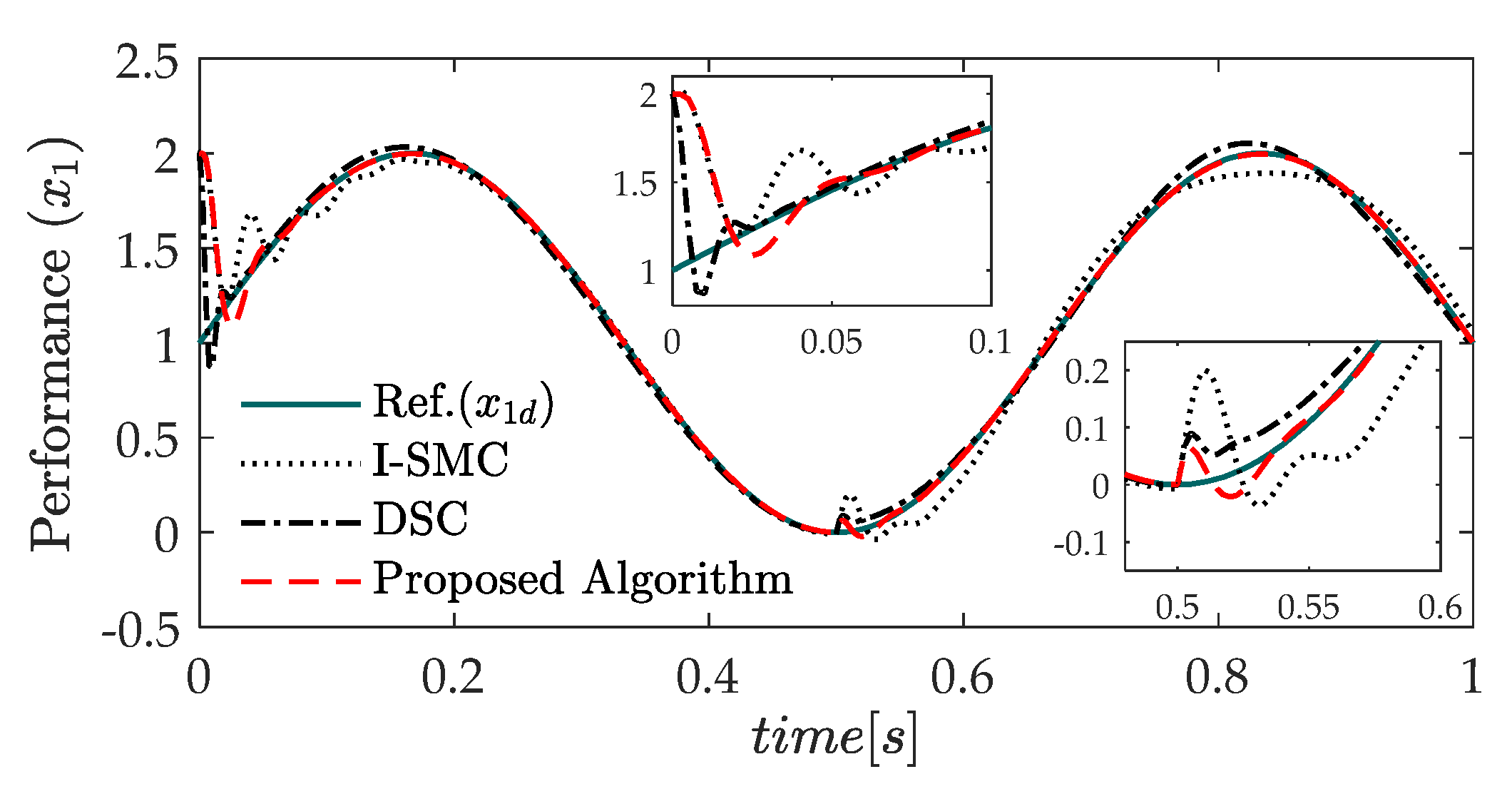
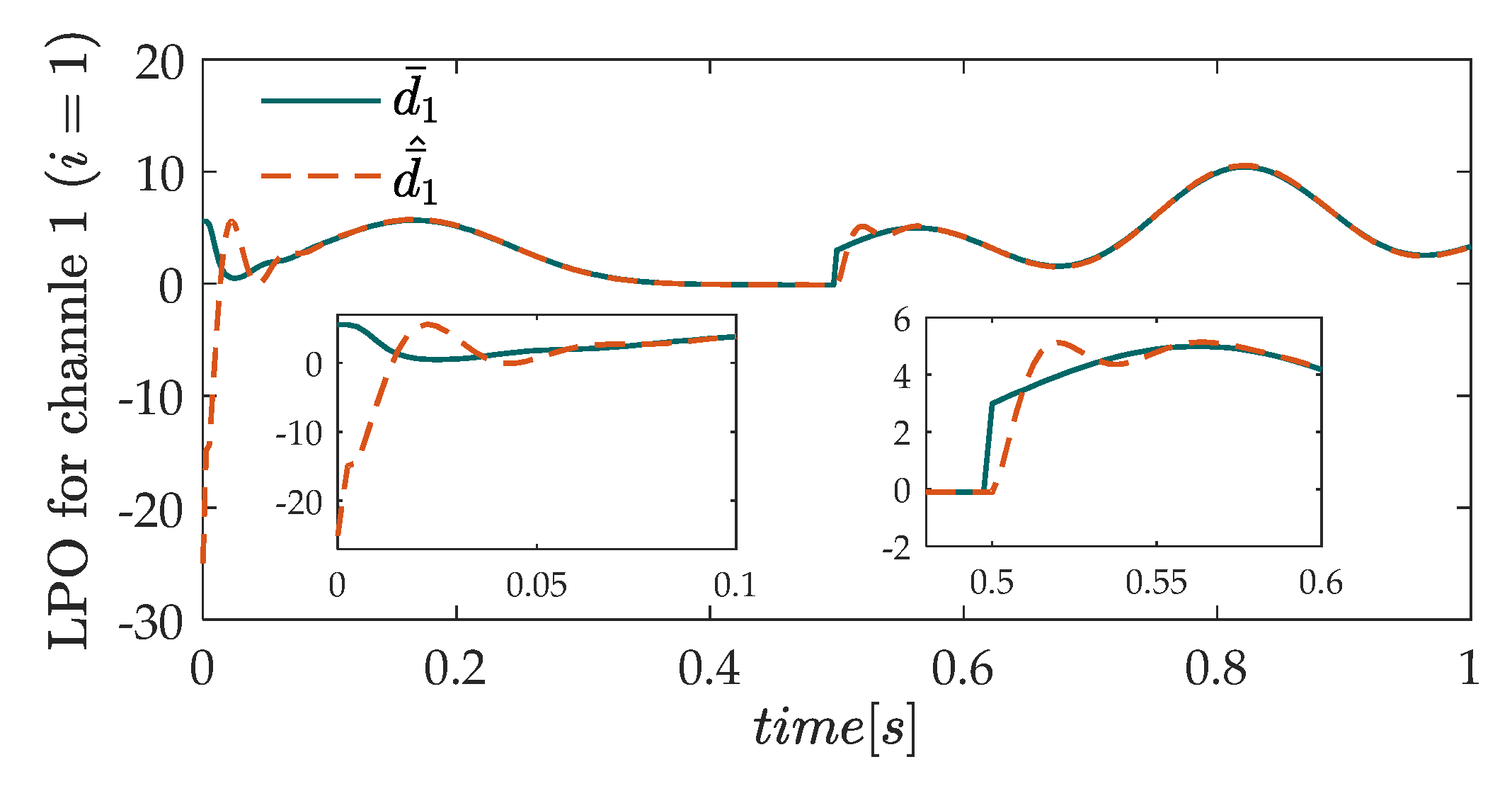
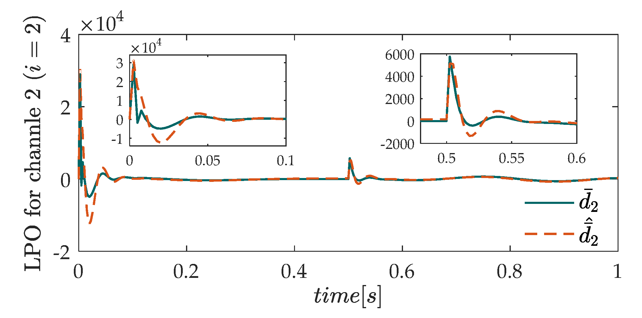
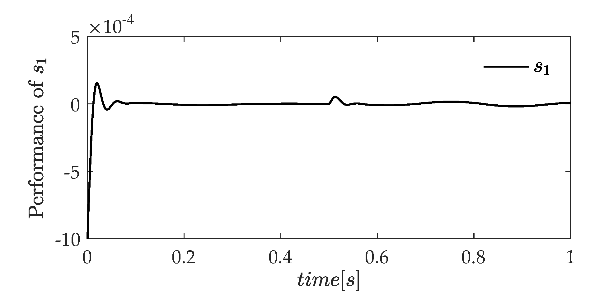
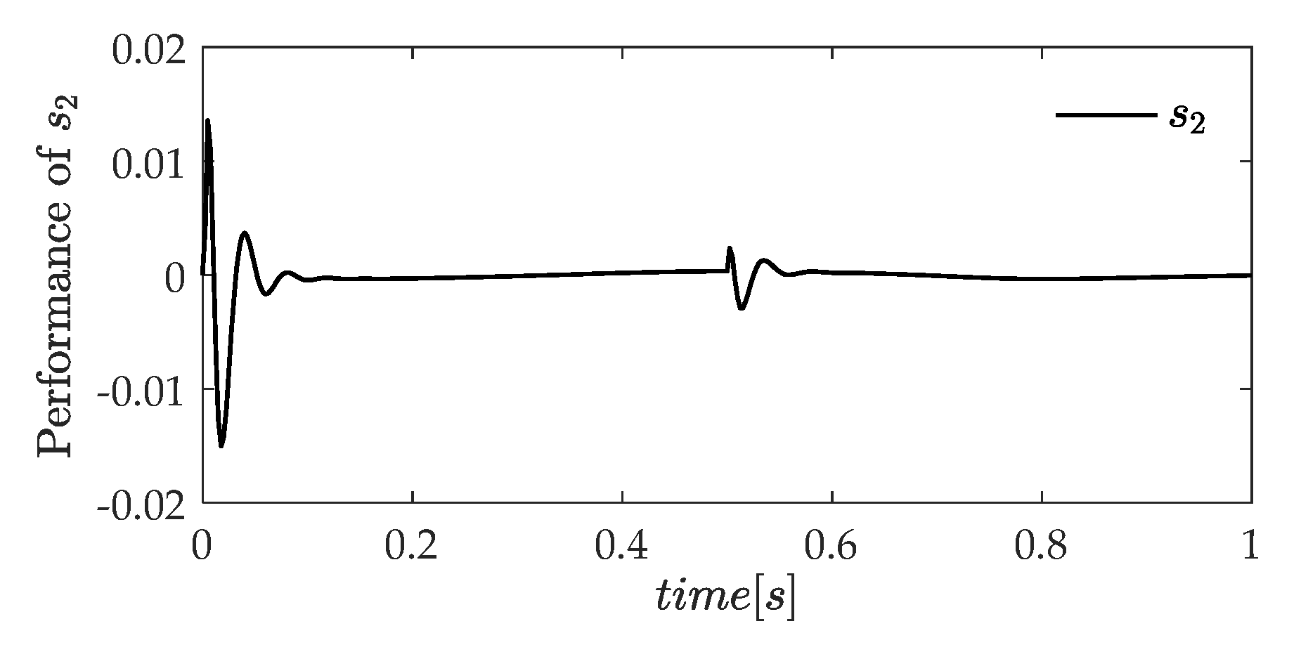
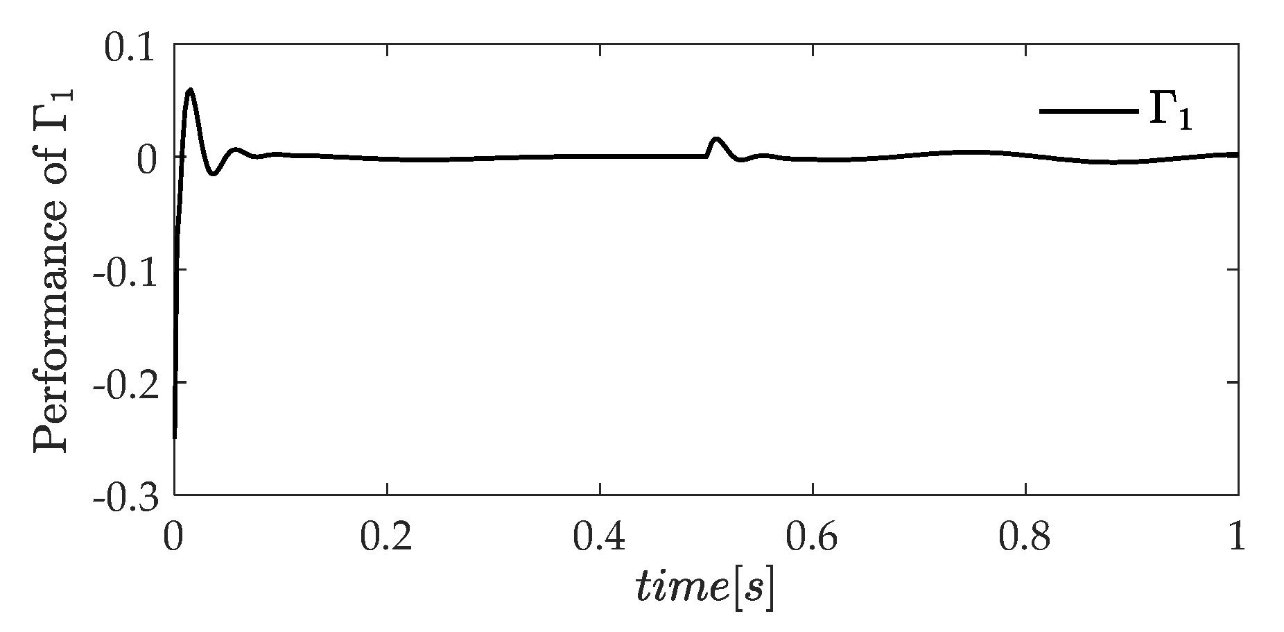
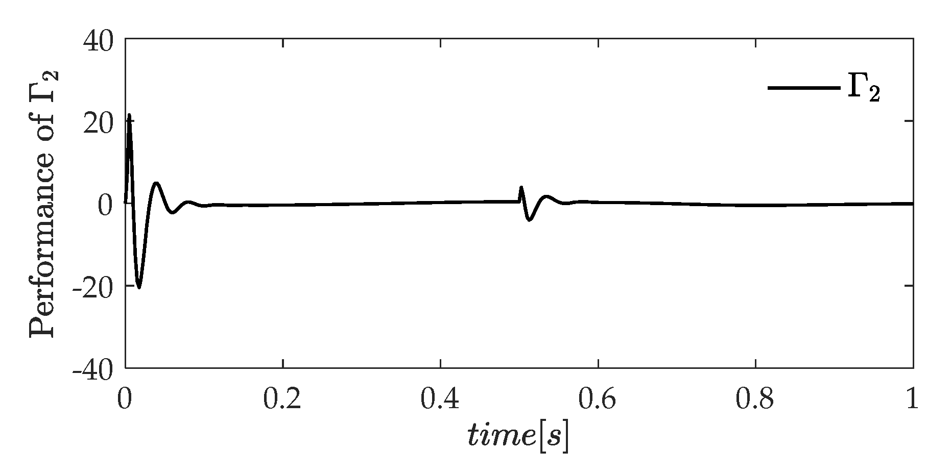
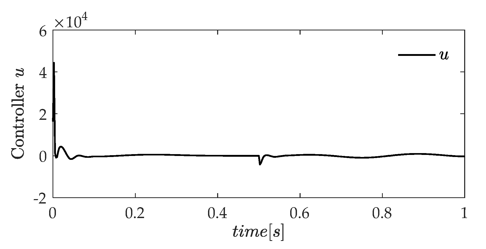
5. Simulation Results and Discussions

In this section, the numerical simulation of an illustrative example is performed and compared with the integral type SMC (I-SMC) in [18] and dynamic surface control method (DSC) in [22] to verify the effectiveness of the proposed algorithm. The mathematical model of an example is considered in [35] as follows.

$$\begin{array}{l}{\dot{x}}_1=x_2+{\xi }_1(\mathbf{x},t)\hspace{0.17em}\hspace{0.17em}\hspace{0.17em}\hspace{0.17em}\\ {\dot{x}}_2=-2x_1-x_2+e^{x_1}+u+{\xi }_2(\mathbf{x},t)\hspace{0.17em}\hspace{0.17em}\hspace{0.17em}\\ y=x_1\end{array}$$

(73)

where ${\xi }_1\left(\mathbf{x},t\right)\hspace{0.17em}$ and ${\xi }_2\left(\mathbf{x},t\right)\hspace{0.17em}$ denote the perturbations/uncertainties given by:

$$\begin{array}{cccc}0<t<0.5s& & & \{\begin{array}{l}{\xi }_1(\mathbf{x},t)\hspace{0.17em}=3.5x_1^4+\sin 3\pi t\\ {\xi }_2(\mathbf{x},t)\hspace{0.17em}\hspace{0.17em}=-x_1+x_2\sin 2\pi t\end{array}\end{array}$$

(74)

$$\begin{array}{cccc}t\ge 0.5s& & & \{\begin{array}{l}{\xi }_1(\mathbf{x},t)\hspace{0.17em}=30+3.5x_1^4+20\sin 8\pi t\\ {\xi }_2(\mathbf{x},t)\hspace{0.17em}=-5x_1+x_2\sin 8\pi t\end{array}\end{array}$$

(75)

The illustrative example is a second order system. Therefore, from the theoretical analysis of the proposed algorithm in Section 3, the controller u is computed by Equation (35), where the sliding surfaces ${\Gamma }_1,{\Gamma }_2$ are obtained from Equation (7) to (9), and lumped disturbance estimations ${\widehat{\overline{d}}}_1,\hspace{0.17em}\hspace{0.17em}{\widehat{\overline{d}}}_2$ are obtained from Equation (37) to (47) with n = 2. The control objective is to derive a control law and LPO so that the system output state, $x_1$, closely tracks the desired trajectory $x_{1d}=1+\sin 3\pi t$. The parameters of the proposed sliding surfaces, ${\Gamma }_i$ and $s_i,\hspace{0.17em}\hspace{0.17em}(i=1,2)$, and switching controller gain are given as

Table 1. Parameters and controller gains of the proposed controller.

Symbol	${\mathit{\lambda }}_1$	${\mathit{\lambda }}_2$	${\mathit{\mu }}_1$	${\mathit{\mu }}_2$	${\mathit{\beta }}_1$	${\mathit{\beta }}_2$	${\mathit{\theta }}_1$	${\mathit{\theta }}_2$	${\mathit{k}}_{\mathit{s}}$	${\mathit{k}}_1$	${\mathit{k}}_2$
Value	250	1300	0.1	0.5	0.001	0.01	0.001	0.07	20	50	80

:

The other parameters of the lumped perturbation observer are chosen as $l_{11}=100$, $\hspace{0.17em}{l}_{12}=400$, $l_{21}=450$, $l_{22}=200\hspace{0.17em},\hspace{0.17em}\hspace{0.17em}{\delta }_1=50,\hspace{0.17em}\hspace{0.17em}{\delta }_2=500$. The initial values are given as $x_1(0)=2$, and $x_2(0)=0$. The simulation results are exhibited from Figure 1, Figure 2, Figure 3, Figure 4, Figure 5, Figure 6, Figure 7 and Figure 8.

From Figure 1, we can see that the output response, $x_1$, of the proposed controller rapidly tracks the desired trajectory, $x_{1d}$, with a minor error, whilst the other controllers as I-SMC and DSC exhibit a poor performance. The estimation of lumped perturbations in the channel 1 and channel 2 of the system (73) are shown in Figure 2 and Figure 3. Obviously, the approximate values ${\widehat{\overline{d}}}_1$ and ${\widehat{\overline{d}}}_2$ fast tracks the true value ${\overline{d}}_1$ and ${\overline{d}}_2$ with a minor error. The trajectories of $s_1$, $s_2$ and ${\Gamma }_1$, ${\Gamma }_2$ well converge to the small region surrounding the origin zero, as exhibited in Figure 4, Figure 5, Figure 6 and Figure 7. In Figure 8, the controller signal u shows a valid performance, excellently eliminating the chattering effect.

6. Conclusions

In this article, we presented a lumped perturbation observer-based control method using a novel extended multiple sliding surface for matched and unmatched uncertain nonlinear systems. In this proposed approach, the sliding surfaces are generated for all channels of the SISO system to approximate the lumped perturbations/uncertainties influencing on the engineering system, without any knowledge of the bound conditions. Following this, an efficient controller combined with the approximated values was derived to solve the control problem excellently. A general stability was proven through the Lyapunov theory. The effectiveness of the proposed controller was demonstrated by an illustrative example. The simulation results show that the proposed method is greatly significant of improving the control performance of the system.

References

1. Precup, R.-E.; Radac, M.-B.; Roman, R.-C.; Petriu, E.M. Model-free sliding mode control of nonlinear systems: Algorithms and experiments. Inf. Sci. 2017, 381, 176–192. [Google Scholar] [CrossRef]
2. Barmish, B.R.; Leitmann, G. On ultimate boundedness control of uncertain systems in the absence of matching condition. IEEE Trans. Autom. Control 1982, 27, 153–158. [Google Scholar] [CrossRef]
3. Arefi, M.M.; Jahed-Motlagh, M.R.; Karimi, H.R. Adaptive Neural Stabilizing Controller for a Class of Mismatched Uncertain Nonlinear Systems by State and Output Feedback. IEEE Trans. Cybern. 2014, 45, 1587–1596. [Google Scholar] [CrossRef] [PubMed]
4. Choi, H.H. An LMI-based switching surface design method for a class of mismatched uncertain systems. IEEE Trans. Autom. Control 2003, 48, 1634–1638. [Google Scholar] [CrossRef]
5. Kim, K.-S.; Park, Y.; Oh, S.-H. Designing robust sliding hyperplanes for parametric uncertain systems: A Riccati approach. Automatica 2000, 36, 1041–1048. [Google Scholar] [CrossRef]
6. Wen, C.-C.; Cheng, C.-C. Design of sliding surface for mismatched uncertain systems to achieve asymptotical stability. J. Frankl. Inst. 2008, 345, 926–941. [Google Scholar] [CrossRef]
7. Zhai, D.; An, L.; Ye, D.; Zhang, Q. Adaptive Reliable H Static Output Feedback Control Against Markovian Jumping Sensor Failures. IEEE Trans. Neural Netw. Learn. Syst. 2018, 29, 631–644. [Google Scholar] [CrossRef]
8. Chang, Y. Adaptive Sliding Mode Control of Multi-Input Nonlinear Systems with Perturbations to Achieve Asymptotical Stability. IEEE Trans. Autom. Control 2009, 54, 2863–2869. [Google Scholar] [CrossRef]
9. Zhai, D.; An, L.; Dong, J.; Zhang, Q. Output feedback adaptive sensor failure compensation for a class of parametric strict feedback systems. Automatica 2018, 97, 48–57. [Google Scholar] [CrossRef]
10. Mehdi, H.; Mohammad, J.Y. Performance enhanced model reference adaptive control through switching non-quadratic Lyapunov functions. Syst. Control Lett. 2015, 76, 47–55. [Google Scholar]
11. Lu, C.; Hua, L.; Zhang, X.; Wang, H.; Guo, Y. Adaptive Sliding Mode Control Method for Z-Axis Vibrating Gyroscope Using Prescribed Performance Approach. Appl. Sci. 2020, 10, 4779. [Google Scholar] [CrossRef]
12. Choi, H.H. LMI-Based Sliding Surface Design for Integral Sliding Mode Control of Mismatched Uncertain Systems. IEEE Trans. Autom. Control 2007, 52, 736–742. [Google Scholar] [CrossRef]
13. Abo-Hammour, Z.S.; Abu Arqub, O.; Alsmadi, O.; Momani, S.; Alsaedi, A. An Optimization Algorithm for Solving Systems of Singular Boundary Value Problems. Appl. Math. Inf. Sci. 2014, 8, 2809–2821. [Google Scholar] [CrossRef]
14. Yang, J.; Mu, A. Adaptive Fixed Time Control for Generalized Synchronization of Mismatched Dynamical Systems with Parametric Estimations. IEEE Access 2019, 7, 114426–114439. [Google Scholar] [CrossRef]
15. Mahmoud, M.S.; Al-Rayyah, A. Adaptive control of systems with mismatched non-linearities and time-varying delays using state measurements. IET Control Theory Appl. 2010, 4, 27–36. [Google Scholar] [CrossRef]
16. Zhai, D.; An, L.; Dong, J.; Zhang, Q. Robust Adaptive Fuzzy Control of a Class of Uncertain Nonlinear Systems with Unstable Dynamics and Mismatched Disturbances. IEEE Trans. Cybern. 2017, 48, 3105–3115. [Google Scholar] [CrossRef]
17. Rahmani, M.; Komijani, H.; Ghanbari, A.; Ettefagh, M.M. Optimal novel super-twisting PID sliding mode control of a MEMS gyroscope based on multi-objective bat algorithm. Microsyst. Technol. 2018, 24, 2835–2846. [Google Scholar] [CrossRef]
18. Xu, Q. Digital Integral Terminal Sliding Mode Predictive Control of Piezoelectric-Driven Motion System. IEEE Trans. Ind. Electron. 2015, 63, 3976–3984. [Google Scholar] [CrossRef]
19. Yu, X.; Kaynak, O. Sliding-Mode Control with Soft Computing: A Survey. IEEE Trans. Ind. Electron. 2009, 56, 3275–3285. [Google Scholar] [CrossRef]
20. Cao, W.-J.; Xu, J.-X. Nonlinear Integral-Type Sliding Surface for both Matched and Unmatched Uncertain Systems. IEEE Trans. Autom. Control 2004, 49, 1355–1360. [Google Scholar] [CrossRef]
21. Huang, A.-C.; Chen, Y.-C. Adaptive Sliding Control for Single-Link Flexible-Joint Robot with Mismatched Uncertainties. IEEE Trans. Control Syst. Technol. 2004, 12, 770–775. [Google Scholar] [CrossRef]
22. Shieh, H.-J.; Shyu, K.-K. Nonlinear sliding-mode torque control with adaptive backstepping approach for induction motor drive. IEEE Trans. Ind. Electron. 1999, 46, 380–389. [Google Scholar] [CrossRef]
23. Estrada, A.; Fridman, L. Quasi-continuous HOSM control for systems with unmatched perturbations. Automatica 2010, 46, 1916–1919. [Google Scholar] [CrossRef]
24. Swaroop, D.; Hedrick, J.; Yip, P.P.; Gerdes, J. Dynamic surface control for a class of nonlinear systems. IEEE Trans. Autom. Control 2000, 45, 1893–1899. [Google Scholar] [CrossRef] [Green Version]
25. Li, J.; Zhang, Q.; Yan, X.-G.; Spurgeon, S. Observer-Based Fuzzy Integral Sliding Mode Control For Nonlinear Descriptor Systems. IEEE Trans. Fuzzy Syst. 2018, 26, 2818–2832. [Google Scholar] [CrossRef] [Green Version]
26. Liu, C.; Liu, G.; Fang, J. Feedback Linearization and Extended State Observer-Based Control for Rotor-AMBs System with Mismatched Uncertainties. IEEE Trans. Ind. Electron. 2017, 64, 1313–1322. [Google Scholar] [CrossRef]
27. Zheng, W.; Li, S.; Wang, J.; Wang, Z. Sliding-mode control for three phase PWM inverter via harmonic disturbance observer. In Proceedings of the 4th Chinese Control Conference (CCC), Hangzhou, China, 28–30 July 2015; pp. 7988–7993. [Google Scholar]
28. Wei, X.; Guo, L. Composite disturbance-observer-based control and terminal sliding mode control for non-linear systems with disturbances. Int. J. Control 2009, 82, 1082–1098. [Google Scholar] [CrossRef]
29. Chen, M.; Chen, W.-H. Sliding mode control for a class of uncertain nonlinear system based on disturbance observer. Int. J. Adapt. Control Signal Process. 2009, 24, 51–64. [Google Scholar] [CrossRef]
30. Lu, Y.-S.; Chiu, C.-W. A stability-guaranteed integral sliding disturbance observer for systems suffering from disturbances with bounded first time derivatives. Int. J. Control Autom. Syst. 2011, 9, 402–409. [Google Scholar] [CrossRef]
31. Wu, S.N.; Sun, X.Y.; Sun, Z.W.; Wu, X.D. Sliding-mode control for staring-mode spacecraft using a disturbance observer. Proc. Inst. Mech. Eng. Part G J. Aerosp. Eng. 2010, 224, 215–224. [Google Scholar] [CrossRef]
32. Chen, W.-H. Disturbance Observer Based Control for Nonlinear Systems. IEEE/ASME Trans. Mechatron. 2004, 9, 706–710. [Google Scholar] [CrossRef] [Green Version]
33. Chen, W.-H.; Ballance, D.; Gawthrop, P.J.; O’Reilly, J. A nonlinear disturbance observer for robotic manipulators. IEEE Trans. Ind. Electron. 2000, 47, 932–938. [Google Scholar] [CrossRef] [Green Version]
34. An, H.; Liu, J.; Wang, C.; Wu, L. Disturbance Observer-Based Antiwindup Control for Air-Breathing Hypersonic Vehicles. IEEE Trans. Ind. Electron. 2016, 63, 3038–3049. [Google Scholar] [CrossRef]
35. Chen, W.-H. Nonlinear Disturbance Observer-Enhanced Dynamic Inversion Control of Missiles. J. Guid. Control Dyn. 2003, 26, 161–166. [Google Scholar] [CrossRef]
36. Ginoya, D.; Shendge, P.D.; Phadke, S.B. Sliding Mode Control for Mismatched Uncertain Systems Using an Extended Disturbance Observer. IEEE Trans. Ind. Electron. 2014, 61, 1983–1992. [Google Scholar] [CrossRef]
37. Yang, J.; Li, S.; Yu, X. Sliding-Mode Control for Systems with Mismatched Uncertainties via a Disturbance Observer. IEEE Trans. Ind. Electron. 2012, 60, 160–169. [Google Scholar] [CrossRef]
38. Ngo, P.D.; Shin, Y.C. Modeling of unstructured uncertainties and robust controlling of nonlinear dynamic systems based on type-2 fuzzy basis function networks. Eng. Appl. Artif. Intell. 2016, 53, 74–85. [Google Scholar] [CrossRef]
39. Kayacan, E. Sliding mode control for systems with mismatched time-varying uncertainties via a self-learning disturbance observer. Trans. Inst. Meas. Control 2018, 41, 2039–2052. [Google Scholar] [CrossRef]
40. Hou, L.; Li, W.; Shen, H.; Li, T. Fuzzy Sliding Mode Control for Systems With Matched and Mismatched Uncertainties/Disturbances Based on ENDOB. IEEE Access 2018, 7, 666–673. [Google Scholar] [CrossRef]
41. Ha, T.; Hong, S.K. Quadcopter Robust Adaptive Second Order Sliding Mode Control Based on PID Sliding Surface. IEEE Access 2018, 6, 66850–66860. [Google Scholar] [CrossRef]
Figure 1. Tracking performance of x 1 .
Mathematics 08 01371 g001
Figure 2. Estimate performance of d ¯ ^ 1 .
Mathematics 08 01371 g002
Figure 3. Estimate performance of d ¯ ^ 2 .
Mathematics 08 01371 g003
Figure 4. Trajectory of s1.
Mathematics 08 01371 g004
Figure 5. Trajectory of s2.
Mathematics 08 01371 g005
Figure 6. Trajectory of Γ 1 .
Mathematics 08 01371 g006
Figure 7. Trajectory of Γ 2 .
Mathematics 08 01371 g007
Figure 8. Controller performance.
Mathematics 08 01371 g008