p-Moment Mittag–Leffler Stability of Riemann–Liouville Fractional Differential Equations with Random Impulses

Abstract

Fractional differential equations with impulses arise in modeling real world phenomena where the state changes instantaneously at some moments. Often, these instantaneous changes occur at random moments. In this situation the theory of Differential equations has to be combined with Probability theory to set up the problem correctly and to study the properties of the solutions. We study the case when the time between two consecutive moments of impulses is exponentially distributed. In connection with the application of the Riemann–Liouville fractional derivative in the equation, we define in an appropriate way both the initial condition and the impulsive conditions. We consider the case when the lower limit of the Riemann–Liouville fractional derivative is fixed at the initial time. We define the so called p-moment Mittag–Leffler stability in time of the model. In the case of integer order derivative the introduced type of stability reduces to the p–moment exponential stability. Sufficient conditions for p–moment Mittag–Leffler stability in time are obtained. The argument is based on Lyapunov functions with the help of the defined fractional Dini derivative. The main contributions of the suggested model is connected with the implementation of impulses occurring at random times and the application of the Riemann–Liouville fractional derivative of order between 0 and 1. For this model the p-moment Mittag–Leffler stability in time of the model is defined and studied by Lyapunov functions once one defines in an appropriate way their Dini fractional derivative.

1. Introduction

Fractional differential equations are considered as a generalization of ordinary differential equations and many results about different types of fractional differential equations are obtained in the literature [1,2,3]. However this is not the situation with fractional impulsive differential equations because of the nonlocal feature. The impulsive effects exist in many evolution processes, when the states change abruptly at certain moments of time. In the literature many authors consider impulsive differential equations with determined impulsive moments [4,5,6]. Since often in a real world problem impulsive perturbations occur at random moments, so it requires combining the Theory of Differential Equations and Probability Theory and to set up a new model [7,8,9].

Several results were obtained in the literature for stochastic differential equations with jumps [10,11] and some results on the qualitative properties of equations with random impulses were obtained [12,13,14]. In the monograph [15], impulsive differential equations with fixed impulses and random amplitude of jumps were studied and ordinary and delay differential equations with random impulses were studied in [16,17,18,19,20], but unfortunately there was some inaccurate applications of real variables and random variables. In [7], the authors set it up appropriately and studied the exponential stability for differential equations with random impulses by Lyapunov direct method and in [21] ordinary and Caputo fractional differential equations of impulses at random times are set up and the stability properties are investigated.

Note the case of deterministic impulses at initially given fixed points in Caputo fractional differential equations was studied in many papers (see the surveys [22,23] and cited therein references). The question concerning Riemann–Liouville fractional differential equations with deterministic impulses is still at an early stage of investigation (see, for example, [24]) and there is nothing on random impulses.

In this paper we study nonlinear fractional differential equations subject to impulses occurring at random moments. We study the case of the Riemann–Liouville (RL) fractional derivative with a fixed lower limit of the derivative at the initial time. In connection with the presence of the RL derivative, we define in an appropriate way both the impulsive conditions and the initial condition. In particular we study the case of exponentially distributed random variables between two consecutive moments of impulses and we study the p-moment stability of the given equation. This type of stability is deeply connected with the application of Mittag–Leffler functions with one parameter. Also, the presence of the RL fractional derivative and its singularity at the initial time leads to excluding this point from the interval of the stability and we define a new type of stability called the p-moment Mittag–Leffler stability in time. We study this type of stability by employing Lyapunov functions. The fractional Dini derivative is defined and it is applied to obtain sufficient conditions for stability.

The main contributions of the paper can be summarized as:

-

The case of impulses occurring at random times is studied when the waiting time between two consecutive impulses is exponentially distributed;

-

The statement of the initial value problem with Riemann–Liouville fractional derivatives of order between 0 and 1 is given in an appropriate way;

-

The p-moment Mittag–Leffler stability in time of the model is defined;

-

The fractional Dini derivative of the Lyapunov function is defined;

-

Sufficient conditions for p-moment Mittag–Leffler stability in time are obtained.

2. Notes on Fractional Calculus

In engineering, the fractional order q is often less than 1, so we restrict our attention to $q\in (0,1)$.

In this paper we will use the following definitions for fractional derivatives and integrals for scalar functions $m:[0,T]\to \mathbb{R}$ with $T\le \infty$:

Definition 1.

Riemann–Liouville fractional integral of order $q\in (0,1)$ (Section 1.4.1.1 [25], or [26])) is

$${}_0{I}_t^{q}m\left(t\right)=\frac{1}{\mathsf{\Gamma }\left(q\right)}\underset{0}{\overset{t}{\int }}\frac{m\left(s\right)}{{(t-s)}^{1-q}}ds,t\in (0,T],$$

where Γ is the Gamma function.

Definition 2.

Riemann–Liouville (RL) fractional derivative of order $q\in (0,1)$ (Section 1.4.1.1 [25], or [26])) is

$${}_0^{RL}{D}_t^{q}m\left(t\right)=\frac{d}{dt}({}_0{I}_t^{1-q}m\left(t\right))=\frac{1}{\mathsf{\Gamma }(1-q)}\frac{d}{dt}\underset{0}{\overset{t}{\int }}{(t-s)}^{-q}m\left(s\right)ds,t\in (0,T].$$

Definition 3.

Grunwald–Letnikov (GL) fractional derivative is given by (see, for example, 1.4.1.2 [25])

$${}_0^{GL}{D}^{q}m\left(t\right)=\underset{h\to 0}{\lim }\frac{1}{h^q}{\displaystyle \sum _{r=0}^{\left[\frac{t}{h}\right]}}{(-1)}^r{}_q{C}_{r}m(t-rh),t\in (0,T],$$

and the Grunwald–Letnikov fractional Dini derivative by

$${}_0^{GL}{D}_{+}^{q}m\left(t\right)=\underset{h\to 0+}{\lim \sup }\frac{1}{h^q}{\displaystyle \sum _{r=0}^{\left[\frac{t}{h}\right]}}{(-1)}^r{}_q{C}_{r}m(t-rh),t\in (0,T],$$

(1)

where ${}_q{C}_r=\frac{q(q-1)\dots (q-r+1)}{r!}$, $r\ge 0$ is an integer and $\left[\frac{t}{h}\right]$ denotes the integer part of the fraction $\frac{t}{h}$.

Remark 1.

In the case of vector functions the RL derivative is taken component-wise, i.e., for the function $x:[0,T]\to {\mathbb{R}}^n:x=(x_1,x_2,\dots ,x_n)$ we have ${}_0^{RL}{D}_t^{q}x\left(t\right)=({}_0^{RL}{D}_t^q{x}_1\left(t\right),{}_0^{RL}{D}_t^q{x}_2\left(t\right),\dots ,{}_0^{RL}{D}_t^q{x}_n\left(t\right))$. Similarly are defined ${}_0{I}_t^{q}x\left(t\right)$ and ${}_0^{GL}{D}^{q}m\left(t\right)$ for a vector function $x\left(t\right)$.

According to [26] if $m\left(t\right)\in C\left(\right[0,T],\mathbb{R})$, $m^{\prime }\left(t\right)$ is integrable in $[0,T]$ and $0<q<1$ then both the RL derivative and the GL derivativeH1 coincide, i.e., ${}_0^{RL}{D}^{q}m\left(t\right)={}_0^{GL}{D}^{q}m\left(t\right)$.

The definitions of the initial condition for fractional differential equations with RL-derivatives are based on the following result:

Lemma 1

([27] Lemma 3). Let $q\in (0,1)$, $0\le t_0<T\le \infty$ and $m\left(t\right)$ be a Lebesque measurable scalar function on $[t_0,T]$.

(a) 

If there exists a.e. a limit $li{m}_{t\to t_0+}\left[{(t-t_0)}^{q-1}m\left(t\right)\right]=c$, then there also exists a limit

$${}_{t_0}{I}_t^{1-q}{m\left(t\right)|}_{t=t_0}:=\underset{t\to t_0+}{\lim }{}_{t_0}{I}_t^{1-q}m\left(t\right)=c\mathsf{\Gamma }\left(q\right).$$

(b) 

If there exists a.e. a limit ${}_{t_0}{I}_t^{1-q}{m\left(t\right)|}_{t=t_0}=b$ and if there exists the limit ${\lim }_{t\to t_0+}\left[{(t-t_0)}^{1-q}m\left(t\right)\right]$, then

$$\underset{t\to t_0+}{\lim }\left[{(t-t_0)}^{1-q}m\left(t\right)\right]=\frac{b}{\mathsf{\Gamma }\left(q\right)}.$$

We introduce the class of functions

$$P{C}_{1-q}([a,b],{\mathbb{R}}^n)=\{x:[a,b]\to \mathbb{R}:{}_a{I}_t^{1-q}x\left(t\right){|}_{t=a}<\infty ,{}_0^{RL}{D}_t^{q}x\left(t\right)\mathrm{exits}\mathrm{for}t\in (a,b]\},$$

where $a,b\in {\mathbb{R}}_{+}:a<b$.

Note that according to Lemma 1 if the function $x\in C((a,b],{\mathbb{R}}^n)$ and the limit ${\lim }_{t\to a}{(t-a)}^{1-q}x\left(t\right)<\infty$ then $x\in P{C}_{1-q}([a,b],{\mathbb{R}}^n)$.

The explicit formula for the solution of the linear scalar problem with the RL fractional derivative is given in the following Proposition:

Proposition 1

(Example 4.1 [27]). The solution of the initial value problem for the the linear RL fractional equation;

$${}_a^{RL}{D}_t^{q}x\left(t\right)=\lambda x\left(t\right)+f\left(t\right),{}_a{I}_t^{1-q}{x\left(t\right)|}_{t=a}=b,$$

(2)

has the following form (formula 4.1.14 [27])

$$x\left(t\right)=\frac{b}{{(t-a)}^{1-q}}{E}_{q,q}\left(\lambda {(t-a)}^q\right)+{\int }_a^t{(t-s)}^{q-1}{E}_{q,q}\left(\lambda {(t-s)}^q\right)f\left(s\right)ds,$$

(3)

where $E_{\alpha ,\beta }\left(z\right)={\sum }_{k=0}^{\infty }\frac{z^k}{\mathsf{\Gamma }(\alpha k+\beta )}$ is the Mittag–Leffler function with two parameters and $\mathsf{\Gamma }(.)$ is the Gamma function.

We will consider some special cases of the function $f\left(t\right)$ in the linear RL fractional Equation (3).

Corollary 1.

The solution of the Cauchy type problem

$${}_0^{RL}{D}_t^{q}x\left(t\right)=x\left(t\right)+\frac{t^{1-q}}{\mathsf{\Gamma }(2-q)}-\frac{t}{\mathsf{\Gamma }\left(2\right)},{}_0{I}_t^{1-q}{x\left(t\right)|}_{t=0}=b,$$

has the following form

$$x\left(t\right)=\frac{b}{t^{1-q}}{E}_{q,q}\left(t^q\right)+t.$$

(4)

Proof. 

According to Equation (2.2.32) [28]

$${\int }_0^t{u}^{q-1}{E}_{q,q}\left(u^q\right)[\frac{{(t-u)}^{1-q}}{\mathsf{\Gamma }(2-q)}-\frac{t-u}{\mathsf{\Gamma }\left(2\right)}]du=t.$$

(5)

Substitute $t-u=s$ then $u=0=>t=s,u=t=>t=0,du=-ds$ and obtain

$${\int }_0^t{(t-s)}^{q-1}{E}_{q,q}\left({(t-s)}^q\right)[\frac{s^{1-q}}{\mathsf{\Gamma }(2-q)}-\frac{s}{\mathsf{\Gamma }\left(2\right)}]ds=t.$$

(6)

From Proposition 1 and Equation (3) we have

$$\begin{array}{cc}\hfill x\left(t\right)& =\frac{b}{t^{1-q}}{E}_{q,q}\left(t^q\right)+{\int }_0^t{(t-s)}^{q-1}{E}_{q,q}\left({(t-s)}^q\right)[\frac{s^{1-q}}{\mathsf{\Gamma }(2-q)}-\frac{s}{\mathsf{\Gamma }\left(2\right)}]ds\hfill \\ \hfill & =\frac{b}{t^{1-q}}{E}_{q,q}\left(t^q\right)+t.\hfill \end{array}$$

(7)

□

Corollary 2.

The solution of the Cauchy type problem

$${}_0^{RL}{D}_t^{q}x\left(t\right)=\lambda x\left(t\right)+\frac{t^{p-1}}{\mathsf{\Gamma }\left(p\right)},{}_0{I}_t^{1-q}{x\left(t\right)|}_{t=0}=b,$$

where $p>0$ has the following form

$$x\left(t\right)=\frac{b}{t^{1-q}}{E}_{q,q}\left(\lambda t^q\right)+t^{q+p-1}{E}_{q,q+p}\left(\lambda t^q\right).$$

(8)

Proof. 

According to Example 2.2.4 [28]

$$\frac{1}{\mathsf{\Gamma }\left(p\right)}{\int }_0^t{u}^{q-1}{(t-u)}^{p-1}{E}_{q,q}\left(\lambda u^q\right)du=t^{q+p-1}{E}_{q,q+p}\left(\lambda t^q\right).$$

(9)

Substitute $t-u=s$ and obtain

$$\frac{1}{\mathsf{\Gamma }\left(p\right)}{\int }_0^t{(t-s)}^{q-1}{E}_{q,q}\left({(t-s)}^q\right)s^{p-1}ds=t^{q+p-1}{E}_{q,q+p}\left(\lambda t^q\right).$$

(10)

From Proposition 1 and Equation (3) we have

$$\begin{array}{cc}\hfill x\left(t\right)& =\frac{b}{t^{1-q}}{E}_{q,q}\left(\lambda t^q\right)+{\int }_0^t{(t-s)}^{q-1}{E}_{q,q}\left(\lambda {(t-s)}^q\right)\frac{s^{p-1}}{\mathsf{\Gamma }\left(p\right)}ds\hfill \\ \hfill & =\frac{b}{t^{1-q}}{E}_{q,q}\left(t^q\right)+t^{q+p-1}{E}_{q,q+p}\left(\lambda t^q\right).\hfill \end{array}$$

(11)

□

Corollary 3.

The solution of the Cauchy type problem

$${}_0^{RL}{D}_t^{q}x\left(t\right)=\lambda x\left(t\right)+t^{p-1}{E}_{q,p}\left(\beta t^q\right),{}_0{I}_t^{1-q}x\left(t\right){|}_{t=0}=b,$$

where $\beta \ne \lambda$ has the following form

$$x\left(t\right)=\frac{b}{t^{1-q}}{E}_{q,q}\left(\lambda t^q\right)+\frac{\beta E_{q,q+p}\left(\beta t^q\right)-\lambda E_{q,q+p}\left(\lambda t^q\right)}{\beta -\lambda }{t}^{q+p-1}.$$

(12)

Proof. 

According to Example 2.2.2 [28]

$${\int }_0^t{s}^{p-1}{E}_{q,p}\left(\beta s^q\right){(t-s)}^{q-1}{E}_{q,q}\left(\lambda {(t-s)}^q\right)ds=\frac{\beta E_{q,q+p}\left(\beta t^q\right)-\lambda E_{q,q+p}\left(\lambda t^q\right)}{\beta -\lambda }{t}^{q+p-1}.$$

(13)

From Proposition 1 and Equation (3) we have

$$\begin{array}{cc}\hfill x\left(t\right)& =\frac{b}{t^{1-q}}{E}_{q,q}\left(\lambda t^q\right)+{\int }_0^t{(t-s)}^{q-1}{E}_{q,q}\left(\lambda {(t-s)}^q\right)s^{p-1}{E}_{q,p}\left(\beta s^q\right)ds\hfill \\ \hfill & =\frac{b}{t^{1-q}}{E}_{q,q}\left(\lambda t^q\right)+\frac{\beta E_{q,q+p}\left(\beta t^q\right)-\lambda E_{q,q+p}\left(\lambda t^q\right)}{\beta -\lambda }{t}^{q+p-1}.\hfill \end{array}$$

(14)

□

We will provide some results for Mittag–Leffler functions which will be used in the main proofs:

$$t^{q-1}{E}_{q,q}\left(\lambda t^q\right)={}_0^{RL}{D}_t^{1-q}{E}_q\left(\lambda t^q\right).$$

$${\int }_0^t{(t-s)}^{q-1}{E}_q\left(s^q\right)ds=\mathsf{\Gamma }\left(q\right)t^q{E}_{q,q+1}\left(t^q\right).$$

From Theorem 10.1 [29]

$$\frac{1}{\mathsf{\Gamma }\left(q\right)}{\int }_0^t{(t-s)}^{q-1}{s}^{q-1}{E}_{q,q}\left(\lambda s^q\right)ds=t^{2q-1}{E}_{q,2q}\left(\lambda t^q\right).$$

From Theorem 10.3 [29]

$${}^{RL}{D}_0^q\left(t^{q-1}{E}_{q,q}\left(\lambda t^q\right)\right)=\lambda t^{q-1}{E}_{q,q}\left(\lambda t^q\right),$$

$$\frac{1}{\mathsf{\Gamma }(1-q)}{\int }_a^t{(t-s)}^{-q}{s}^{q-1}{E}_{q,q}\left(\lambda s^q\right)ds=E_q\left(\lambda t^q\right),$$

$${\left(E_q\left(t\right)\right)}^{\prime }=\frac{1}{q}{E}_{q,q}\left(t\right),$$

$$E_{q,p}\left(t\right)=\frac{1}{\mathsf{\Gamma }\left(p\right)}+t{E}_{q,q+p}\left(t\right).$$

From (1.99) [26] we get

$${\int }_0^t{s}^{p-1}{E}_{q,p}\left(\lambda s^q\right)ds=t^p{E}_{q,p+1}\left(\lambda t^q\right).$$

3. Preliminary Notes and Results for RL Fractional Differential Equations

Consider the initial value problem (IVP) for the system of fractional differential equations (FrDE) with a RL fractional derivative for $0<q<1$,

$${}_0^{RL}{D}^{q}x=f(t,x)\mathrm{for}t>0\mathrm{with}{}_0{I}_t^{1-q}{x\left(t\right)|}_{t=0}=x_0,$$

(15)

where $f\in C[{\mathbb{R}}_{+}\times {\mathbb{R}}^n,{\mathbb{R}}^n]$, and $x_0\in {\mathbb{R}}^n$ is the arbitrary initial data.

We will assume the following condition is satisfied

Hypothesis 1.

For any initial value $x_0\in {\mathbb{R}}^n$ the IVP (15) has an unique solution $x\left(t\right)=x(t;x_0)$ defined for $t\ge 0$.

Some sufficient conditions for global existence of solutions of (15) are given in [26,27,30].

About the fractional order we will assume:

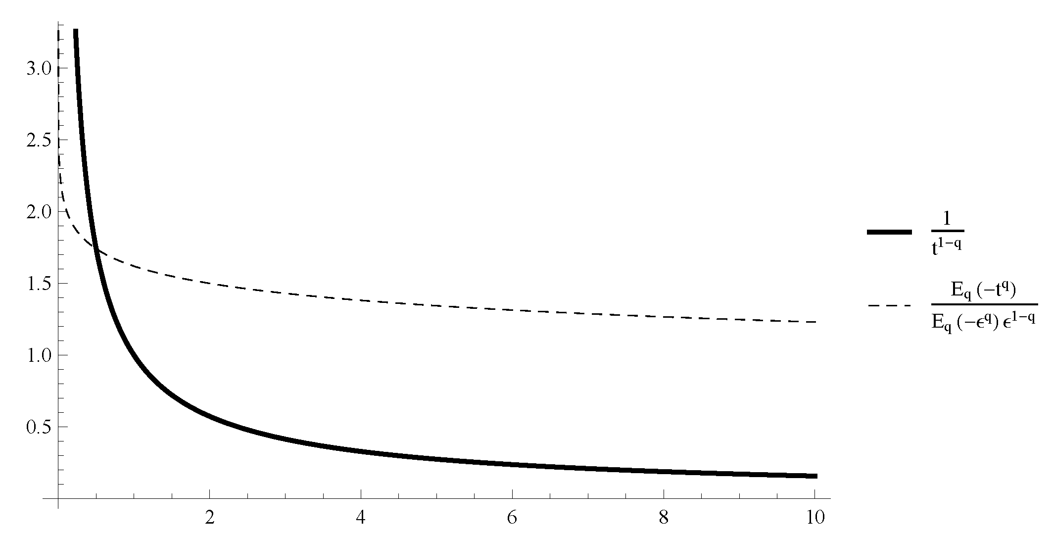
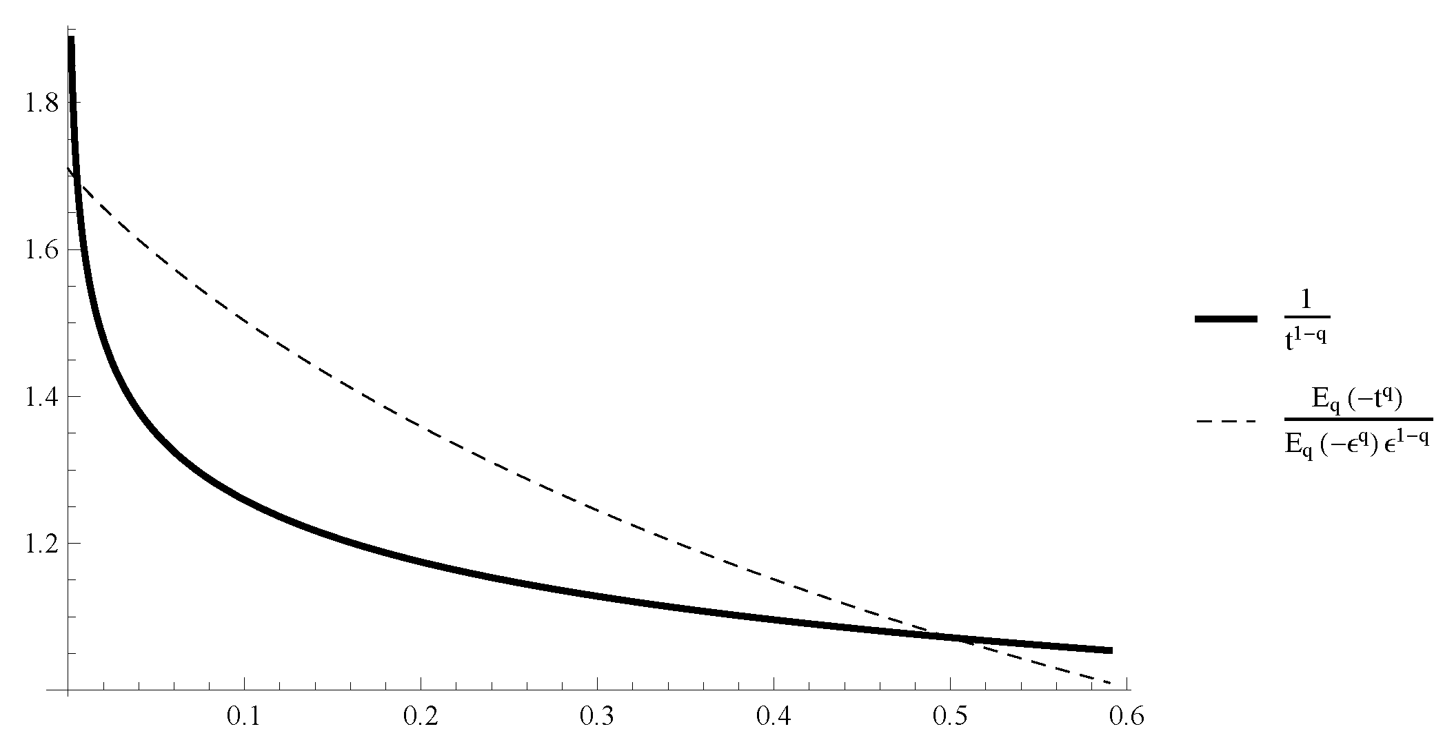
Hypothesis 2.

The number $q\in (0,1)$ is such that for any $ϵ>0$ the equation $\frac{1}{t^{1-q}}=\frac{1}{E_q(-{ϵ}^q){ϵ}^{1-q}}{E}_q(-t^q)$ has only one solution for $t>0$, where $E_{\alpha }\left(z\right)={\sum }_{k=0}^{\infty }\frac{z^k}{\mathsf{\Gamma }(\alpha k+1)}$ is the Mittag–Leffler function with one parameter.

Example 1.

The number $q=0.2$ satisfies condition H2 but the number $q=0.9$ does not. See, for example Figure 1 and Figure 2 for $ϵ=0.5$.

Let the increasing sequence of nonnegative points ${\left\{T_k\right\}}_{k=1}^{\infty }$ be given with $T_0=0$, ${\lim }_{k\to \infty }\left\{T_k\right\}=\infty$. As it is explained in [31] there are two basic types of interpretations of impulses in RL fractional differential equations and two types of impulsive conditions when the RL fractional derivative is used. In this paper we will use a fixed lower limit of the RL fractional derivative at 0 on the whole interval of consideration. Also, we will use the integral form of the initial condition and the impulsive conditions. According to the above we will consider the initial value problem for the RL fractional differential equations (IFrDE) with fixed points of impulses

$$\begin{array}{c}{}_0^{RL}{D}^{q}x\left(t\right)=f(t,x\left(t\right))\mathrm{for}t\in (T_k,T_{k+1}],k=0,1,2,\dots ,\hfill \\ {}_{T_k}{I}_t^{1-q}{x\left(t\right)|}_{t=T_k}=b_{k}x(T_k-0),\mathrm{for}k=1,2,\dots ,\hfill \\ {}_0{I}_t^{1-q}{x\left(t\right)|}_{t=0}=x_0,\hfill \end{array}$$

(16)

where $x_0\in {\mathbb{R}}^n$, $f:[0,\infty )\times {\mathbb{R}}^n\to {\mathbb{R}}^n$.

We will also study the initial value problem for the scalar linear RL fractional differential equations with fixed points of impulses

$$\begin{array}{c}{}_0^{RL}{D}^{q}u=au\left(t\right)+g\left(t\right)\mathrm{for}t\in (T_k,T_{k+1}],k=0,1,2,\dots ,\hfill \\ {}_{T_k}{I}_t^{1-q}{u\left(t\right)|}_{t=T_k}=b_{k}u(T_k-0),\mathrm{for}k=1,2,\dots ,\hfill \\ {}_0{I}_t^{1-q}{u\left(t\right)|}_{t=0}=u_0,\hfill \end{array}$$

(17)

where $u_0\in \mathbb{R}$, $g:[0,\infty )\to \mathbb{R}$, $a,b_k,k=1,2,\dots ,$ are constants.

There is an explicit formula of the solution of (17) given in [31]:

Lemma 2

([31]). The IVP for the linear scalar RL fractional differential equation with impulses (17) has an exact solution $u\in P{C}_{1-q}([0,\infty ),\mathbb{R})$ given by

$$\begin{array}{cc}\hfill u\left(t\right)& =B_k\frac{E_{q,q}\left(a{(t-T_k)}^q\right)}{{(t-T_k)}^{1-q}}+{\int }_{T_k}^t\frac{E_{q,q}\left(s{(t-s)}^q\right)}{{(t-s)}^{1-q}}(g\left(s\right)+{\displaystyle \sum _{j=1}^k}{h}_j\left(s\right))ds,\hfill \\ \hfill & fort\in (T_k,T_{k+1}],k=0,1,2,\dots ,\hfill \end{array}$$

(18)

where $B_0=u_0$,

$$\begin{array}{cc}\hfill h_k\left(t\right)& =\frac{q}{\mathsf{\Gamma }(1-q)}{\displaystyle \underset{T_{k-1}}{\overset{T_k}{\int }}}\{B_{k-1}\frac{E_{q,q}\left({(s-T_{k-1})}^q\right)}{{(s-T_{k-1})}^{1-q}{(t-s)}^{1+q}}\hfill \\ \hfill & +{\int }_{T_{k-1}}^s\frac{E_{q,q}\left(a{(s-\sigma )}^q\right)}{{(s-\sigma )}^{1-q}{(t-s)}^{1+q}}(g\left(\sigma \right)+{\displaystyle \sum _{j=1}^{k-1}}{h}_j\left(\sigma \right))d\sigma \}ds,t\in [T_k,\infty ),\hfill \\ \hfill & k=1,2,\dots ,\hfill \end{array}$$

(19)

and

$$\begin{array}{c}{B}_k=b_k\{B_{k-1}\frac{E_{q,q}\left(a{(T_k-T_{k-1})}^q\right)}{{(T_k-T_{k-1})}^{1-q}}\hfill \\ +{\int }_{T_{k-1}}^{t_k}\frac{E_{q,q}\left(a{(T_k-s)}^q\right)}{{(t_k-s)}^{1-q}}(g\left(s\right)+{\displaystyle \sum _{j=1}^{k-1}}{h}_j\left(s\right))ds\},fork=1,2,3,\dots .\hfill \end{array}$$

(20)

Consider the following linear scalar IVP

$$\begin{array}{c}{}_0^{RL}{D}^{q}u=au\left(t\right)\mathrm{for}t\in (T_k,T_{k+1}],k=0,1,2,\dots ,\hfill \\ {}_{T_k}{I}_t^{1-q}{u\left(t\right)|}_{t=T_k}=0,\mathrm{for}k=1,2,\dots ,\hfill \\ {}_0{I}_t^{1-q}{u\left(t\right)|}_{t=0}=u_0,\hfill \end{array}$$

(21)

where $u_0\in \mathbb{R},a\in \mathbb{R}$.

As a special case of Lemma 2 we obtain

Lemma 3.

The IVP for the linear scalar RL fractional differential equation with impulses (21) has an exact solution $u\in P{C}_{1-q}([0,\infty ),\mathbb{R})$, given by

$$u\left(t\right)=\{\begin{array}{cc}{u}_0\frac{E_{q,q}\left(a{t}^q\right)}{t^{1-q}},\hfill & t\in (0,T_1],\hfill \\ \frac{q{u}_0}{\mathsf{\Gamma }(1-q)}{\int }_{T_1}^t\frac{E_{q,q}\left(a{(t-s)}^q\right)}{{(t-s)}^{1-q}}{h}_1\left(s\right)ds,\hfill & t\in (T_1,T_2],\hfill \\ \frac{q{u}_0}{\mathsf{\Gamma }(1-q)}{\int }_{T_k}^t\frac{E_{q,q}\left(a{(t-s)}^q\right)}{{(t-s)}^{1-q}}(h_1\left(s\right)+\frac{q}{\mathsf{\Gamma }(1-q)}{\sum }_{j=2}^k{h}_j\left(s\right))ds,\hfill & t\in (T_k,T_{k+1}],k=2,3,\dots .\hfill \end{array}$$

where

$$h_k\left(t\right)=\{\begin{array}{cc}{\int }_0^{T_1}\frac{E_{q,q}\left(a{s}^q\right)}{{(t-s)}^{1+q}{s}^{1-q}}ds,\hfill & t>T_1,\hfill \\ {\int }_{T_{k-1}}^{T_k}{\int }_{T_{k-1}}^s\frac{E_{q,q}\left(a{(s-\sigma )}^q\right)}{{(t-s)}^{1+q}{(s-\sigma )}^{1-q}}(h_1\left(\sigma \right)+\frac{q}{\mathsf{\Gamma }(1-q)}{\sum }_{j=2}^{k-1}{h}_j\left(\sigma \right))d\sigma ds,\hfill & t>T_k,k=2,3,\dots .\hfill \end{array}$$

in the case $a<0$ the following estimate

$$\left|u\left(t\right)\right|\le \{\begin{array}{cc}\frac{|u_0|}{t^{1-q}\mathsf{\Gamma }\left(q\right)},\hfill & t\in (0,T_1],\hfill \\ \frac{|u_0|\pi Csc\left[\pi q\right]}{t^{1-q}\mathsf{\Gamma }\left(q\right)\mathsf{\Gamma }(1-q)},\hfill & t\in (T_1,T_2],\hfill \\ \frac{|u_0|\pi Csc\left(\pi q\right)}{t^{1-q}\mathsf{\Gamma }\left(q\right)\mathsf{\Gamma }(1-q)}(n-1)(1+\frac{\pi Csc\left(\pi q\right)}{\mathsf{\Gamma }\left(q\right)\mathsf{\Gamma }(1-q)}),\hfill & t\in (T_n,T_{n+1}],n=2,3,\dots \hfill \end{array}$$

holds.

Proof. 

The first part of the claim directly follows from Lemma 2 with $g\left(t\right)\equiv 0,b_k=0,k=1,2,\dots$.

Let $a<0$. Then $E_{q,q}\left(a{t}^q\right)\le E_{q,q}\left(0\right)=\frac{1}{\mathsf{\Gamma }\left(q\right)},t\ge 0$ and

$$h_1\left(t\right)={\int }_0^{T_1}\frac{E_{q,q}\left(a{s}^q\right)}{{(t-s)}^{1+q}{s}^{1-q}}ds\le \frac{1}{q\mathsf{\Gamma }\left(q\right)}\frac{T_1^{q-1}}{{(t-T_1)}^q},t>T_1,$$

(22)

$$\begin{array}{cc}\hfill h_2\left(t\right)& \le \frac{1}{\mathsf{\Gamma }\left(q\right)}{\int }_{T_1}^{T_2}{\int }_{T_1}^s\frac{1}{{(t-s)}^{1+q}{(s-\sigma )}^{1-q}}{h}_1\left(\sigma \right))d\sigma ds\hfill \\ \hfill & \le \frac{T_1^{q-1}}{q{\mathsf{\Gamma }}^2\left(q\right)}{\int }_{T_1}^{T_2}{\int }_{T_1}^s\frac{1}{{(t-s)}^{1+q}{(s-\sigma )}^{1-q}{(\sigma -T_1)}^q})d\sigma ds\hfill \\ \hfill & \le \frac{T_1^{q-1}\pi Csc\left(\pi q\right)}{q{\mathsf{\Gamma }}^2\left(q\right)}{\int }_{T_1}^{T_2}\frac{1}{{(t-s)}^{1+q}}ds\le \frac{T_1^{q-1}\pi Csc\left(\pi q\right)}{q^2{\mathsf{\Gamma }}^2\left(q\right){(t-T_2)}^q},t>T_2,\hfill \end{array}$$

(23)

$$\begin{array}{cc}\hfill h_3\left(t\right)& ={\int }_{T_2}^{T_3}{\int }_{T_2}^s\frac{E_{q,q}\left(a{(s-\sigma )}^q\right)}{{(t-s)}^{1+q}{(s-\sigma )}^{1-q}}(h_1\left(\sigma \right)+\frac{q}{\mathsf{\Gamma }(1-q)}{h}_2\left(\sigma \right))d\sigma ds\hfill \\ \hfill & \le \frac{T_1^{q-1}\pi Csc\left(\pi q\right)}{q^2{\mathsf{\Gamma }}^2\left(q\right){(t-T_3)}^q}(1+\frac{\pi Csc\left(\pi q\right)}{\mathsf{\Gamma }\left(q\right)\mathsf{\Gamma }(1-q)}),t>T_3,\hfill \end{array}$$

(24)

and by induction we get

$$h_n\left(t\right)\le \frac{T_1^{q-1}\pi Csc\left(\pi q\right)}{q^2{\mathsf{\Gamma }}^2\left(q\right){(t-T_n)}^q}(n-2)(1+\frac{\pi Csc\left(\pi q\right)}{\mathsf{\Gamma }\left(q\right)\mathsf{\Gamma }(1-q)}),t>T_n,n=3,4,\dots .$$

(25)

From inequalities (22)–(25), the formula for the solution $u\left(t\right)$ and the equality ${\int }_{T_k}^t\frac{1}{{(t-s)}^{1-q}{(s-T_k)}^q}=\pi Csc\left(\pi q\right),t>T_k$ we obtain the estimate for $u\left(t\right)$ in the claim. □

4. RL Fractional Differential Equations with Random Impulses

Now we define fractional differential equations with random points of impulses and random amplitude of impulses. Let the probability space ($\mathsf{\Omega },\mathcal{F},P$) be given. Let ${\left\{{\tau }_k\right\}}_{k=1}^{\infty }$ be a sequence of independent exponentially distributed random variables with a parameter $\lambda >0$, that are defined on the sample space $\mathsf{\Omega }$. The random variables ${\tau }_k$ define the time between two consecutive impulses of the considered impulsive fractional differential equation.

Assume ${\sum }_{k=1}^{\infty }{\tau }_k=\infty$ with probability 1.

We will assume the following condition is satisfied

Hypothesis 3.

The random variables ${\left\{{\tau }_k\right\}}_{k=1}^{\infty }$ are independent exponentially distributed random variables with a parameter λ.

Define the sequence of random variables ${\left\{{\xi }_k\right\}}_{k=0}^{\infty }$ such that ${\xi }_0\equiv 0$ and ${\xi }_k={\sum }_{i=1}^k{\tau }_i,k=1,2,\dots$.

We note that ${\left\{{\xi }_k\right\}}_{k=0}^{\infty }$ is an increasing sequence of random variables. The random variable ${\xi }_n$ will be called the waiting time and it gives the arrival time of the n-th impulse.

Let the points $t_k$ be arbitrary values of the corresponding random variables ${\tau }_k,k=1,2,\dots$. Define the increasing sequence of points $T_k={\sum }_{i=1}^k{t}_i$, $k=1,2,3\dots$ that are values of the random variables ${\xi }_k$.

Consider the initial value problem for the system of IFrDE with fixed points of impulses (16). The solution of the impulsive fractional differential equation with fixed moments of impulses (16) depends not only on the initial value $x_0$ but also on the moments of impulses $T_k,k=1,2,\dots$, i.e., the solution depends on the chosen arbitrary values $t_k$ of the random variables ${\tau }_k,k=1,2,\dots$. We denote the solution of the initial value problem (16) by $x(t;x_0,\left\{T_k\right\})$.

The set of all solutions $x(t;x_0,\left\{T_k\right\})$ of the initial value problem for the impulsive fractional differential Equation (16) for any values $t_k$ of the random variables ${\tau }_k,k=1,2,\dots$ generates a stochastic process with state space ${\mathbb{R}}^n$. We denote it by $x(t;x_0,\left\{{\tau }_k\right\})$ and we will say that it is a solution of the following initial value problem for the system of impulsive fractional differential equations with random moments of impulses (RIFrDE)

$$\begin{array}{c}{}_0^{RL}{D}^{q}x\left(t\right)=f(t,x\left(t\right))\mathrm{for}{\xi }_k<t<{\xi }_{k+1},k=0,1,\dots ,\hfill \\ {}_{{\xi }_k}{I}_t^{1-q}{x\left(t\right)|}_{t={\xi }_k}=I_k\left(x({\xi }_k-0)\right),\mathrm{for}k=1,2,\dots ,\hfill \\ {}_0{I}_t^{1-q}{x\left(t\right)|}_{t=0}=x_0,\hfill \end{array}$$

(26)

where $x_0\in {\mathbb{R}}^n$.

Definition 4.

Suppose $t_k$ is a value of the random variable ${\tau }_k$, $k=1,2,3,\dots$ and $T_k={\sum }_{i=1}^k{t}_i,k=1,2,\dots$. Then the solution $x(t;x_0,\left\{T_k\right\})$ of the IVP for the IFrDE with fixed points of impulses formally written by

$$\begin{array}{c}{}_0^{RL}{D}^{q}x\left(t\right)=f(t,x\left(t\right))for{T}_k<t<T_{k+1},k=0,1,\dots ,\hfill \\ {}_{T_k}{I}_t^{1-q}{x\left(t\right)|}_{t=T_k}=I_k\left(x(T_k-0)\right),fork=1,2,\dots ,\hfill \\ {}_0{I}_t^{1-q}{x\left(t\right)|}_{t=0}=x_0,\hfill \end{array}$$

(27)

is called a sample path solution of the IVP for the RIFrDE (26) (here $T_0=0$).

Any sample path solution $x(t;x_0,\left\{T_k\right\})\in P{C}_{1-q}[(T_k,T_{k+1}],{\mathbb{R}}^n)$, $k=0,1,2,\dots$.

Definition 5.

A stochastic process $x(t;x_0,\left\{{\tau }_k\right\})$ with an uncountable state space ${\mathbb{R}}^n$ is said to be a solution of the IVP for the system of RIFrDE (26) if for any values $t_k$ of the random variable ${\tau }_k$, $k=1,2,3,\dots$ and $T_k={\sum }_{i=1}^k{t}_i,k=1,2,\dots$ the corresponding function $x(t;x_0,\left\{T_k\right\})$ is a sample path solution of the IVP for RIFrDE (26).

According to Definition 5 and Lemma 3 any solution of the IVP for the scalar linear fractional differential equation with random moments of impulses:

$$\begin{array}{c}{}_0^{RL}{D}^{q}u=-au\mathrm{for}t\ge 0,{\xi }_k<t<{\xi }_{k+1},\hfill \\ {}_{{\xi }_k}{I}_t^{1-q}{u\left(t\right)|}_{t={\xi }_k}=0,\mathrm{for}k=1,2,\dots ,\hfill \\ {}_0{I}_t^{1-q}{u\left(t\right)|}_{t=0}=u_0,\hfill \end{array}$$

(28)

where $u_0\in \mathbb{R}$, $a>0$, will have a sample path solution satisfying the IVP (21).

Definition 6.

The stochastic processes $y\left(t\right)$ and $u\left(t\right)$ satisfy the inequality $y\left(t\right)\le u\left(t\right)$ for $t\in J\subset \mathbb{R}$ if the state space of the stochastic processes $v\left(t\right)=y\left(t\right)-u\left(t\right)$ is $(-\infty ,0]$.

Consider the events

$$S_k\left(t\right)=\{\omega \in \mathsf{\Omega }:{\xi }_k\left(\omega \right)<t<{\xi }_{k+1}\left(\omega \right)\},k=1,2,\dots .$$

Lemma 4

([7]). The probability that there will be exactly k impulses until time t, $t\ge 0$ is given by $P\left(S_k\left(t\right)\right)=\frac{{\lambda }^k{t}^k}{k!}{e}^{-\lambda t}.$

Lemma 5.

Let the hypothesis 3 be satisfied.

Then for any positive number $ϵ>0$ the solution $u(t;u_0,\left\{{\tau }_k\right\})$ of the IVP for the linear RIFrDE (28) satisfies the inequality

$$E\left(\right|u(t;u_0,\left\{{\tau }_k\right\})|)\le |u_0|\frac{\lambda }{t^{1-q}\mathsf{\Gamma }\left(q\right)}\frac{\pi Csc\left(\pi q\right)}{\mathsf{\Gamma }(1-q)}(1+\frac{\pi Csc(\pi q}{\mathsf{\Gamma }\left(q\right)\mathsf{\Gamma }(1-q)}),t\ge 0,$$

where $E(.)$ is the expected value.

Proof. 

Choose arbitrary values $t_k$ of the random variables ${\tau }_k$, $k=1,2,\dots$. Define the increasing sequence of points $T_k={\sum }_{i=1}^k{t}_i,k=1,2,,3\dots$ that are values of the random variables ${\xi }_k$ and consider the IVP for the linear IFrDE with fixed points of impulses (21). The explicit formula of the sample path solution of (28) is given in Lemma 3. The set of all solutions $u(t;u_0,\left\{T_k\right\})$ of the IVP (21) for any values $t_k$ of the random variables ${\tau }_k$ generates a continuous stochastic process $u(t;u_0,\left\{{\tau }_k\right\})$. □

According to Lemmas 3 and 4, the independence of the random variables ${\tau }_k$, $k=1,2,\dots$ we see that the expected value of the solution of the IVP for the scalar linear RIFrDE (21) satisfies

$$\begin{array}{c}E\left(\right|u(t;u_0,\left\{{\tau }_k\right\})\left|\right)={\displaystyle \sum _{k=0}^{\infty }}E\left(|u(t;T_0,u_0,\left\{{\tau }_k\right\})\left|\right|S_k\left(t\right)\right)P\left(S_k\left(t\right)\right)\hfill \\ \le \frac{|u_0|}{t^{1-q}\mathsf{\Gamma }\left(q\right)}P\left(S_0\left(t\right)\right)+\frac{|u_0|\pi Csc\left[\pi q\right]}{t^{1-q}\mathsf{\Gamma }\left(q\right)\mathsf{\Gamma }(1-q)}P\left(S_1\left(t\right)\right)\hfill \\ +{\displaystyle \sum _{k=2}^{\infty }}\left|u_0\right|\left((k-1)\frac{\pi Csc\left(\pi q\right)}{t^{1-q}{\mathsf{\Gamma }}^2\left(q\right)\mathsf{\Gamma }(1-q)}\right(1+\frac{\pi Csc(\pi q}{\mathsf{\Gamma }\left(q\right)\mathsf{\Gamma }(1-q)}\left)\right)P\left(S_k\left(t\right)\right)\hfill \\ \le \frac{|u_0|}{t^{1-q}\mathsf{\Gamma }\left(q\right)}{e}^{-\lambda t}+\frac{|u_0|\pi Csc\left[\pi q\right]}{t^{1-q}\mathsf{\Gamma }\left(q\right)\mathsf{\Gamma }(1-q)}\lambda t{e}^{-\lambda t}\hfill \\ +|u_0|\frac{\pi Csc\left(\pi q\right)}{t^{1-q}{\mathsf{\Gamma }}^2\left(q\right)\mathsf{\Gamma }(1-q)}(1+\frac{\pi Csc(\pi q}{\mathsf{\Gamma }\left(q\right)\mathsf{\Gamma }(1-q)})e^{-\lambda t}{\displaystyle \sum _{k=2}^{\infty }}(k-1)\frac{{\lambda }^k{t}^k}{k!}\hfill \\ \le |u_0|\frac{e^{-\lambda t}}{t^{1-q}\mathsf{\Gamma }\left(q\right)}\frac{\pi Csc\left(\pi q\right)}{\mathsf{\Gamma }(1-q)}(1+\frac{\pi Csc(\pi q}{\mathsf{\Gamma }\left(q\right)\mathsf{\Gamma }(1-q)})\lambda e^{\lambda t}\mathrm{for}t\ge 0.\hfill \end{array}$$

(29)

5. p-moment Mittag–Leffler Stability in Time for RIFrDE

We will introduce p-moment stability of the RIFrDE (26). This type of stability is deeply connected with the application of Mittag–Leffler functions with one parameter. Also, the presence of the RL fractional derivative and its singularity at the initial time leads to excluding this point from the interval of the stability. We will call the new type of stability the p-moment Mittag–Leffler stability in time.

Definition 7.

Let $p>0$. Then the RIFrDE (26) is said to be p-moment Mittag–Leffler stable in time if for any $ϵ>0$ and any initial value $x_0\in {\mathbb{R}}^n$ there exists a constant $\alpha >0$ such that

$$E\left[\right||x(t;x_0,\left\{{\tau }_k\right)\}{\left)\right||}^p]<\alpha ||x_0{\left|\right|}^p{E}_q(-t^q),forallt>ϵ,$$

where $x(t;x_0,\left\{{\tau }_k\right\})$ is the solution of the IVP for the RIFrDE (26).

In this section we will use Lyapunov functions to obtain sufficient conditions for the p-moment exponential stability of the trivial solution of the nonlinear impulsive random system impulses occurring at random moments (26).

We now introduce the class $\mathsf{\Lambda }$ of Lyapunov functions which will be used to investigate the stability properties of the zero solution of the system RIFrDE (16).

Definition 8.

Let $J\subset {\mathbb{R}}_{+}$ be a given interval and $\Delta \subset {\mathbb{R}}^n,0\in \Delta$ be a given set. We will say that the function $V(t,x):J\times \Delta \to {\mathbb{R}}_{+}$, $V(t,0)\equiv 0$ belongs to the class $\mathsf{\Lambda }(J,\Delta )$ if it is continuous on $J\times \Delta$ and locally Lipschitzian with respect to its second argument.

We will use Lyapunov functions $V(t,x)$ from the class $\mathsf{\Lambda }\left(\right[0,T],\Delta )$ and their fractional Dini derivatives along trajectories of solutions of the system FrDE (15) defined by:

$$D_{\left(15\right)}^{q}V(t,x)=\underset{h\to 0^{+}}{\lim \sup }\frac{1}{h^q}\{V(t,x)-{\displaystyle \sum _{r=1}^{\left[\frac{t}{h}\right]}}{(-1)}^{r+1}{}_q{C}_{r}V(t-rh,x-h^{q}f(t,x))\},$$

(30)

where ${}_q{C}_r=\frac{q(q-1)(q-2)\dots (q-r+1)}{r!}$, $t\in (0,T)$, $x\in \Delta$, and there exists $h_1>0$ such that $t-h\in [0,T)$, $x-h^{q}f(t,x)\in \Delta$ for $0<h\le h_1$.

Note the formula (30) is similar to the Grunwald–Letnikov fractional Dini derivative of a function given by (1).

Example 2.

Let $V\in \mathsf{\Lambda }(\mathbb{R},\mathbb{R})$ be $V(t,x)=m\left(t\right)x^2$ where $m\in C^1({\mathbb{R}}_{+},{\mathbb{R}}_{+})$. Use (30) to obtain the fractional Dini derivative of V, namely

$$\begin{array}{c}{D}_{\left(15\right)}^{q}V(t,x)\hfill \\ =\underset{h\to 0^{+}}{\lim \sup }\frac{1}{h^q}\{m\left(t\right)x^2-{\displaystyle \sum _{r=1}^{\left[\frac{t}{h}\right]}}{(-1)}^{r+1}{}_q{C}_{r}m(t-rh){(x-h^{q}f(t,x))}^2\}\hfill \\ =\underset{h\to 0^{+}}{\lim \sup }\frac{1}{h^q}\{m\left(t\right)x^2+(x^2-2x{h}^{q}f(t,x)+h^{2q}{f}^2(t,x)){\displaystyle \sum _{r=1}^{\left[\frac{t}{h}\right]}}{(-1)}^r{}_q{C}_{r}m(t-rh)\}\hfill \\ =\underset{h\to 0^{+}}{\lim \sup }\frac{1}{h^q}\{m\left(t\right)\left(h^{q}f(t,x)\right)(2x-h^{q}f(t,x))+x^2{\displaystyle \sum _{r=0}^{\left[\frac{t}{h}\right]}}{(-1)}^r{}_q{C}_{r}m(t-rh)\hfill \\ +2x{h}^{q}f(t,x){\displaystyle \sum _{r=0}^{\left[\frac{t}{h}\right]}}{(-1)}^{r+1}{}_q{C}_{r}m(t-rh)-h^{2q}{f}^2(t,x)){\displaystyle \sum _{r=0}^{\left[\frac{t}{h}\right]}}{(-1)}^{r+1}{}_q{C}_{r}m(t-rh)\}\hfill \\ =2xm\left(t\right)f(t,x)+x^2{}_0^{RL}{D}^q\left(m\right(t\left)\right).\hfill \end{array}$$

In the special case $f(t,x)=xp\left(t\right)$ we obtain

$$D_{\left(15\right)}^{q}V(t,x)=x^2(2m\left(t\right)g\left(t\right)+{}_0^{RL}{D}^q(m\left(t\right)).$$

(31)

Note the fractional Dini derivative depends significantly not only on the order q of the fractional differential equation but also on the initial time (0 in our case).

Remark 2.

We note that if condition (H1) is satisfied then the sample path solution of the IVP for the RIFrDE (26) exists for all $t\ge 0$ provided that the times between two consecutive impulses $t_k$ are such that $\sum t_k=\infty$.

In the case when the Lyapunov function is only continuous we obtain the following sufficient condition for the studied stability type:

Theorem 1.

Let the following conditions be satisfied:

1. 

Hypotheses 1,2,3 hold.

2. 

The function $V\in \mathsf{\Lambda }({\mathbb{R}}_{+},{\mathbb{R}}^n)$ and

(i) for any $ϵ>0$ there exist positive constants $a,b>0$ depending on ϵ such that ${a\left|\right|x\left|\right|}^p\le V(t,x)\le {b\left|\right|x\left|\right|}^p$ for $t>ϵx\in {\mathbb{R}}^n;$

(ii) there exists a constant $m\ge 0$ such that the inequality

$$D_{\left(15\right)}^{q}V(t,x)\le -mV(t,x),fort\ge 0,x\in {\mathbb{R}}^n$$

holds;

(iii) there exists a positive constant $c>0$ such that for any function x such that $t^{1-q}{x\left(t\right)|}_{t=0}=x_0$ the limit

$$t^{1-q}{V(t,x\left(t\right))|}_{t=0}=c\left|\right|x_0{\left|\right|}^p$$

(32)

holds.

Then the system of RIFrDE (26) is p-moment Mittag–Leffler stable.

Proof. 

Let $x_0\in {\mathbb{R}}^n$ be an arbitrary initial value and the stochastic process $x_{\tau }\left(t\right)=x(t;x_0,\left\{{\tau }_k\right\})$ be a solution of the initial value problem for the RIFrDE (26).

Let $ϵ>0$ be an arbitrary number and $t_k$ be arbitrary values of the random variables ${\tau }_k$, $k=1,2,\dots$. Then $T_k={\sum }_{i=1}^k{t}_i,k=1,2,\dots$ are values of the random variables ${\xi }_k$. Thus the corresponding function $x\left(t\right)=x(t;x_0,\left\{T_k\right\})$ is a sample path solution of the IVP for RIFrDE (26), i.e., $x\left(t\right)=x(t;x_0,\left\{T_k\right\})$ is a solution of the IVP for the IFrDE with fixed points of impulses (16).

Let $v\left(t\right)=V(t,x(t\left)\right)$. Then for $t\in (T_k,T_{k+1}],k=0,1,2,\dots ,$ (here $T_0=0$), we obtain

$$\begin{array}{cc}\hfill v\left(t\right)& -{\displaystyle \sum _{r=1}^{\left[\frac{t}{h}\right]}}{(-1)}^{r+1}qCrv(t-rh)\hfill \\ \hfill & =\{V(t,x\left(t\right))-{\displaystyle \sum _{r=1}^{\left[\frac{t}{h}\right]}}{(-1)}^{r+1}{}_q{C}_{r}V(t-rh,x\left(t\right)-h^{q}f(t,x\left(t\right))\}\hfill \\ \hfill & +{\displaystyle \sum _{r=1}^{\left[\frac{t}{h}\right]}}{(-1)}^{r+1}{}_q{C}_r\{V(t-rh,x\left(t\right)-h^{q}f(t,x\left(t\right))-V(t-rh,x(t-rh))\}.\hfill \end{array}$$

(33)

Since $x\left(t\right)\in P{C}_{1-q}([T_k,T_{k+1}],{\mathbb{R}}^n)$ from (28) we have

$$\begin{array}{cc}\hfill {}_0^{RL}{D}_{+}^{q}x\left(t\right)& ={}_0^{GL}{D}_{+}^{q}x\left(t\right)\hfill \\ \hfill & =\underset{h\to 0+}{\lim \sup }\frac{1}{h^q}[x\left(t\right)-{\displaystyle \sum _{r=1}^{\left[\frac{t}{h}\right]}}{(-1)}^{r+1}{}_q{C}_{r}x(t-rh)]=f(t,x\left(t\right)),\hfill \end{array}$$

or

$$x\left(t\right)-h^{q}f(t,x\left(t\right))=S_k(x\left(t\right),h)+\mathsf{\Lambda }\left(h^q\right),$$

(34)

with $\frac{\mathsf{\Lambda }\left(h^q\right)}{h^q}\to 0$ as $h\to 0$ where $S_k(x\left(t\right),h)={\sum }_{r=1}^{\left[\frac{t}{h}\right]}{(-1)}^{r+1}{}_q{C}_{r}x(t-rh).$

Therefore, since V is locally Lipschitzian in its second argument with a Lipschitz constant $L>0$ we obtain

$$\begin{array}{c}{\displaystyle \sum _{r=1}^{\left[\frac{t}{h}\right]}}{(-1)}^{r+1}qCr\{V(t-rh,x\left(t\right)-h^{q}f(t,x\left(t\right))-V(t-rh,x(t-rh))\}\hfill \\ \le L\left|\right|{\displaystyle \sum _{r=1}^{\left[\frac{t}{h}\right]}}{(-1)}^{r+1}{}_q{C}_r(S_k(x(t),h)k+\mathsf{\Lambda }\left(h^q\right)-x(t-rh))\left|\right|\hfill \\ \le L\left|\right|{\displaystyle \sum _{r=1}^{\left[\frac{t}{h}\right]}}{(-1)}^{r+1}{}_q{C}_r{\displaystyle \sum _{j=1}^{\left[\frac{t}{h}\right]}}{(-1)}^{j+1}{}_q{C}_{j}x(t-jh)\hfill \\ -{\displaystyle \sum _{r=1}^{\left[\frac{t}{h}\right]}}{(-1)}^{r+1}{}_q{C}_{r}x(t-rh)\left|\right|+L|\mathsf{\Lambda }\left(h^q\right)|\sum _{r=1}^{\left[\frac{t}{h}\right]}{}_q{C}_r\hfill \\ =L\left|\right|({\displaystyle \sum _{r=0}^{\left[\frac{t}{h}\right]}}{(-1)}^{r+1}{}_q{C}_r)({\displaystyle \sum _{j=1}^{\left[\frac{t}{h}\right]}}{(-1)}^{r+1}{}_q{C}_{j}x(t-jh))\left|\right|+L|\mathsf{\Lambda }\left(h^q\right)|{\displaystyle \sum _{r=1}^{\left[\frac{t}{h}\right]}}{}_q{C}_r.\hfill \end{array}$$

(35)

Now substitute (35) in (33), divide both sides by $h^q$, take the limit as $h\to 0^{+}$, use (28) and ${\sum }_{r=0}^{\infty }{}_q{C}_r{z}^r={(1+z)}^q$ if $\left|z\right|\le 1$, use condition 2(i) and we have

$$\begin{array}{c}{}_0^{GL}{D}_{+}^{q}v\left(t\right)\le D_{\left(15\right)}^{q}V(t,x)+L\underset{h\to 0+}{\lim }\frac{\mathsf{\Lambda }\left(h^q\right)}{h^q}\underset{h\to 0+}{\lim }{\displaystyle \sum _{r=1}^{\left[\frac{t}{h}\right]}}{}_q{C}_r\hfill \\ +L\underset{h\to 0^{+}}{\lim }\sup \left|\right|\left({\displaystyle \sum _{r=0}^{\left[\frac{t}{h}\right]}}{(-1)}^r{}_q{C}_r\right)\left(\frac{1}{h^q}{\displaystyle \sum _{j=1}^{\left[\frac{t}{h}\right]}}{(-1)}^r{}_q{C}_{j}x(t-jh)\right)\left|\right|\hfill \\ \le -mv\left(t\right),t\in (T_k,T_{k+1}].\hfill \end{array}$$

(36)

Also,

$$\begin{array}{c}{t}^{1-q}{v\left(t\right)|}_{t=0}=t^{1-q}{V(t,x\left(t\right))|}_{t=0}\le c\left|\right|x_0{\left|\right|}^p,\hfill \\ {(t-T_k)}^{1-q}v\left(t\right){{|}_{t=T_k}=t^{1-q}V(t,x\left(t\right))\frac{{(t-T_k)}^{1-q}}{t^{1-q}}|}_{t=T_k}\hfill \\ =t^{1-q}V(t,x\left(t\right)){{|}_{t=T_k}\frac{{(t-T_k)}^{1-q}}{t^{1-q}}|}_{t=T_k}=0.\hfill \end{array}$$

(37)

Therefore, from (36), (37) and Lemma 1 it follows that the function $v\left(t\right)$ satisfies the linear impulsive fractional differential inequalities with fixed points of impulses

$$\begin{array}{c}{}_0^{RL}{D}_{+}^{q}v\left(t\right)\le -mv\left(t\right)\mathrm{for}{T}_k<t<T_{k+1}\hfill \\ {}_{T_k}{I}_t^{1-q}{v\left(t\right)|}_{t=T_k}=0,k=1,2,\dots ,\hfill \\ {}_0{I}_t^{1-q}{v\left(t\right)|}_{t=0}=c\left|\right|x_0{\left|\right|}^p.\hfill \end{array}$$

(38)

According to Definition 4 the function $v\left(t\right)$ is a sample path solution and it generates a stochastic process $v(t;c|\left|x_0\right|{|}^p,\left\{{\tau }_k\right\})$ with state space ${\mathbb{R}}^n$.

From conditions (H2), 2(i), Definition 4, Lemmas 3 and 5 we obtain the inequalities

$$\begin{array}{c}E\left(\right||x(t;x_0,\left\{{\tau }_k\right\}){\left|\right|}^p)=\frac{1}{a}E\left(a\right||x(t;x_0,\left\{{\tau }_k\right\}){\left|\right|}^p)\hfill \\ \le \frac{1}{a}E\left(V(t,x(t;x_0,\left\{{\tau }_k\right\}))\right)\le \frac{1}{a}E\left(v\right(t;c\left|\right|x_0{\left|\right|}^p,\left\{{\tau }_k\right\}\left)\right)\hfill \\ \le \frac{1}{a}c\left|\right|x_0{\left|\right|}^p\frac{\lambda }{t^{1-q}\mathsf{\Gamma }\left(q\right)}\frac{\pi Csc\left(\pi q\right)}{\mathsf{\Gamma }(1-q)}(1+\frac{\pi Csc\left(\pi q\right)}{\mathsf{\Gamma }\left(q\right)\mathsf{\Gamma }(1-q)})\hfill \\ \le K\left|\right|x_0{\left|\right|}^p{E}_q(-t^q),t>ϵ,\hfill \end{array}$$

(39)

where $K=\frac{1}{a}c\frac{\lambda }{\mathsf{\Gamma }\left(q\right)}\frac{\pi Csc\left(\pi q\right)}{\mathsf{\Gamma }(1-q)}(1+\frac{\pi Csc(\pi q}{\mathsf{\Gamma }\left(q\right)\mathsf{\Gamma }(1-q)})$.

Inequality (39) proves the p-moment exponential stability. □

Example 3.

Consider the scalar RF fractional differential equation with random impulses

$$\begin{array}{c}{}_0^{RL}{D}^{0.2}x\left(t\right)=f(t,x\left(t\right))for{\xi }_k<t<{\xi }_{k+1},k=0,1,\dots ,\hfill \\ {}_{{\xi }_k}{I}_t^{0.8}{x\left(t\right)|}_{t={\xi }_k}=I_k\left(x({\xi }_k-0)\right),fork=1,2,\dots ,\hfill \\ {}_0{I}_t^{0.8}{x\left(t\right)|}_{t=0}=x_0,\hfill \end{array}$$

(40)

where $x_0\in {\mathbb{R}}^n$, $f(t,x)=-x(1+\frac{{}_0^{RL}{D}^{0.2}{\left(\frac{t}{t+1}\right)}^{0.8}}{{\left(\frac{t}{t+1}\right)}^{1-q}})$ with

$${}_0^{RL}{D}^{0.2}{\left(\frac{t}{t+1}\right)}^{0.8}=\left(1.6\right)t^{0.6}\mathsf{\Gamma }\left(1.8\right)({}_2{F}_1[0.8,1.8,2.6,-t]-0.9t{}_2{F}_1[1.8,2.8,3.6,-t]),$$

where the regularized hypergeometric function ${}_2{F}_1[q,b,c,z]=\frac{1}{\mathsf{\Gamma }\left(b\right)\mathsf{\Gamma }(c-b)}{\int }_0^1{s}^{b-1}{(1-s)}^{c-b-1}{(1-sz)}^{-a}ds$.

According to Example 1 the hypothesis 2 is satisfied with $c=\frac{1}{{ϵ}^{0.8}{E}_{0.2}(-{ϵ}^{0.2})}$ where $ϵ>0$ is an arbitrary number.

Let $V(t,x)={\left(\frac{t}{t+1}\right)}^{0.8}{x}^2$.

Then for any $t>ϵ$ we have $1\ge \frac{t}{t+1}\ge \frac{ϵ}{ϵ+1}$ and $x^2\ge V(t,x)={\left(\frac{t}{t+1}\right)}^{0.8}{x}^2\ge {\left(\frac{ϵ}{ϵ+1}\right)}^{0.8}{x}^2$, i.e., condition 2(i) of Theorem 1 is satisfied.

Also,

$$\underset{t\to 0}{\lim }{t}^{0.8}V(t,x\left(t\right))=\underset{t\to 0}{\lim }{t}^{0.8}{\left(\frac{t}{t+1}\right)}^{0.8}{x}^2=\underset{t\to 0}{\lim }{\left(t^{0.8}x\left(t\right)\right)}^2\underset{t\to 0}{\lim }\frac{1}{{(t+1)}^{0.8}}=x_0^2,$$

i.e., condition 2(iii) of Theorem 1 is satisfied.

According to Example 2 we have

$$D_{\left(15\right)}^{q}V(t,x)=2x{\left(\frac{t}{t+1}\right)}^{0.8}f(t,x)+x^2{}_0^{RL}{D}^{0.2}{\left(\frac{t}{t+1}\right)}^{0.8}\le -2{\left(\frac{t}{t+1}\right)}^{0.8}{x}^2=-2V(t,x),$$

i.e., condition 2(ii) of Theorem 1 is satisfied.

According to Theorem 1 the RIFrDE (40) is p-moment Mittag–Leffler stable, i.e., its solution satisfies

$$E\left[\right||x(t;x_0,\left\{{\tau }_k\right\}){\left|\right|}^p]<\alpha ||x_0{\left|\right|}^p{E}_q(-t^{0.2}),forallt>ϵ,$$

with $\alpha =\frac{\lambda {(1+ϵ)}^{0.8}}{{ϵ}^{1.6}}\frac{\pi Csc\left(0.2\pi \right)}{E_{0.2}(-{ϵ}^{0.2})\mathsf{\Gamma }\left(0.2\right)\mathsf{\Gamma }\left(0.8\right)}(1+\frac{\pi Csc\left(0.2\pi \right)}{\mathsf{\Gamma }\left(0.2\right)\mathsf{\Gamma }\left(0.8\right)})=2\frac{\lambda {(1+ϵ)}^{0.8}}{{ϵ}^{1.6}{E}_{0.2}(-{ϵ}^{0.2})}$.

6. Conclusions

In this paper the RL fractional differential equation is studied when the impulses occur at random times and the waiting time between two consecutive times of impulses is exponentially distributed. We combine the Theory of Differential Equations with Probability Theory to set up the problem and to study the properties of the solutions. In connection with the application of the RL fractional derivative in the equation, we define in an appropriate way both the initial condition and the impulsive conditions. We define p-moment Mittag–Leffler stability in time of the model and obtain some sufficient conditions. The argument is based on Lyapunov functions with the help of the fractional Dini derivative. In further work we hope to consider a number of directions:

(i)

When the waiting time between two consecutive impulses is generalized to Erlang distribution, to Log-normal distribution, etc.

(ii)

When the model of the RL fractional differential equation is generalized to various other types of delays.

References

- Agarwal, R.; Benchohra, M.; Slimani, B.A. Existence results for differential equations with fractional order and impulses. Mem. Differ. Equ. Math. Phys. 2008, 44, 1–21. [Google Scholar]
- Baleanu, D.; Mustafa, O.G. On the global existence of solutions to a class of fractional differential equations. Comput. Math. Appl. 2010, 59, 1835–1841. [Google Scholar]
- Devi, J.V.; Rae, F.A.M.; Drici, Z. Variational Lyapunov method for fractional differential equations. Comput. Math. Appl. 2012, 64, 2982–2989. [Google Scholar]
- Feckan, M.; Zhou, Y.; Wang, J. On the concept and existence of solution for impulsive fractional differential equations. Commun. Nonlinear Sci. Numer. Simul. 2012, 17, 3050–3060. [Google Scholar] [CrossRef]
- Hristova, S. Qualitative Investigations and Approximate Methods for Impulsive Differential Equations; Nova Science Publ.: Hauppauge, NY, USA, 2009. [Google Scholar]
- Hristova, S. Integral stability in terms of two measures for impulsive functional differential equations. Math. Comput. Modell. 2010, 51, 100–108. [Google Scholar] [CrossRef]
- Agarwal, R.; Hristova, S.; O’Regan, D. Exponential stability for differential equations with random impulses at random times. Adv. Diff. Equ. 2013, 2013. [Google Scholar] [CrossRef] [Green Version]
- Sanz-Serna, J.M.; Stuart, A.M. Ergodicity of dissipative differential equations subject to random impulses. J. Diff. Equ. 1999, 155, 262–284. [Google Scholar] [CrossRef] [Green Version]
- Wang, J.R.; Feckan, M.; Zhou, Y. Random Noninstantaneous Impulsive Models for Studying Periodic Evolution Processes in Pharmacotherapy. Math. Model. Appl. Nonl. Dynam. 2016, 14, 87–107. [Google Scholar]
- Wu, S.; Hang, D.; Meng, X. p-Moment Stability of Stochastic Equations with Jumps. Appl. Math. Comput. 2004, 152, 505–519. [Google Scholar]
- Wu, H.; Sun, J. p-Moment Stability of Stochastic Differential Equations with Impulsive Jump and Markovian Switching. Automatica 2006, 42, 1753–1759. [Google Scholar] [CrossRef]
- Naghshtabrizi, P.; Hespanha, J.P.; Teel, A.R. Exponential stability of impulsive systems with application to uncertain sampled-data systems. Syst. Control Lett. 2008, 57, 378–385. [Google Scholar] [CrossRef] [Green Version]
- Smalfuss, B. Attractors for nonautonomous and random dynamical systems perturbed by impulses. Discrete Contin. Dyn. Syst. 2003, 9, 727–744. [Google Scholar] [CrossRef]
- Wu, S. The Euler scheme for random impulsive differential equations. Appl. Math. Comput. 2007, 191, 164–175. [Google Scholar]
- Samoilenko, A.; Stanzhytskyi, O. Qualitative and Asymptotic Analysis of Differential Equations with Random Perturbations; World Scientific: Singapore, 2011. [Google Scholar]
- Anguraj, A.; Wu, S.; Vinodkumar, A. Existence and exponential stability of semilinear functional differential equations with random impulses under non-uniqueness. Nonlin. Anal. TMA 2011, 74, 331–342. [Google Scholar] [CrossRef]
- Anguraj, A.; Vinodkumar, A. Existence, uniqueness and stability results of random impulsive semilinear differential systems. Nonlin. Anal. Hybrid Syst. 2010, 4, 475–483. [Google Scholar] [CrossRef]
- Wu, S.J.; Meng, X.Z. Boundedness of nonlinear differential systems with impulsive effect on random moments. Acta Math. Appl. Sin. 2004, 20, 147–154. [Google Scholar] [CrossRef]
- Wu, S.J.; Duan, Y.R. Oscillation, stability, and boundedness of second-order differential systems with random impulses. Comput. Math. Appl. 2005, 49, 1375–1386. [Google Scholar]
- Wu, S.J.; Guo, X.L.; Zhou, Y. p-Moment stability of functional differential equations with random impulses. Comput. Math. Appl. 2006, 52, 1683–1694. [Google Scholar]
- Agarwal, R.P.; Hristova, S.; O’Regan, D. Non-Instantaneous Impulses in Differential Equations; Springer: New York, NY, USA, 2017. [Google Scholar]
- Agarwal, R.; Hristova, S.; O’Regan, D. A survey of Lyapunov functions, stability and impulsive Caputo fractional differential equations. Fract. Calc. Appl. Anal. 2016, 19, 290–318. [Google Scholar] [CrossRef]
- Wang, J.R.; Feckan, M.; Zhou, Y. A survey on impulsive fractional differential equations. Fract. Calc. Appl. Anal. 2016, 19, 806–831. [Google Scholar] [CrossRef]
- Hristova, S.G.; Tersian, S.A. Scalar linear impulsive Riemann–Liouville fractional differential equations with constant delay–explicit solutions and finite time stability. Demonstr. Math. 2020, 53, 121–130. [Google Scholar] [CrossRef]
- Das, S. Functional Fractional Calculus; Springer: Berlin/Heidelberg, Germany, 2011. [Google Scholar]
- Podlubny, I. Fractional Differential Equations; Academic Press: San Diego, CA, USA, 1999. [Google Scholar]
- Kilbas, A.A.; Srivastava, H.M.; Trujillo, J.J. Theory and Applications of Fractional Differential Equations; Elsevier: Amsterdam, The Netherlands, 2006. [Google Scholar]
- Mathai, A.M. Mittag–Leffler Functions and Fractional Calculus. In Special Functions for Applied Scientists; Springer: New York, NY, USA, 2008; pp. 79–134. [Google Scholar] [CrossRef]
- Haubold, H.J.; Mathai, A.M.; Saxena, R.K. Mittag–Leffler Functions and their applications. J. Appl. Math. 2011, 2011, 298628. [Google Scholar] [CrossRef] [Green Version]
- Lakshmikantham, V.; Leela, S.; Devi, J.V. Theory of Fractional Dynamical Systems; Cambridge Scientific Publishers: Cambridge, UK, 2009. [Google Scholar]
- Agarwal, R.; Hristova, S.; O’Regan, D. Exact solutions of linear Riemann–Liouville fractional differential equations with impulses. Rocky Mt. J. Math. 2020, 50, 779–791. [Google Scholar] [CrossRef]
© 2020 by the authors. Licensee MDPI, Basel, Switzerland. This article is an open access article distributed under the terms and conditions of the Creative Commons Attribution (CC BY) license (http://creativecommons.org/licenses/by/4.0/).