Fourier-Spectral Method for the Phase-Field Equations
by
 , , ,
, , ,
Sungha Yoon
1, 
Darae Jeong
2,
Chaeyoung Lee
1,
Hyundong Kim
1,
Sangkwon Kim
1,
Hyun Geun Lee
3 and
Junseok Kim
1,* 1
Department of Mathematics, Korea University, Seoul 02841, Korea
2
Department of Mathematics, Kangwon National University, Gangwon-do 24341, Korea
3
Department of Mathematics, Kwangwoon University, Seoul 01897, Korea
*
Author to whom correspondence should be addressed.
Mathematics 2020, 8(8), 1385; https://0-doi-org.brum.beds.ac.uk/10.3390/math8081385
Submission received: 5 July 2020
/
Revised: 15 August 2020
/
Accepted: 17 August 2020
/
Published: 18 August 2020
(This article belongs to the Special Issue Open Source Codes for Numerical Analysis)
Abstract
:In this paper, we review the Fourier-spectral method for some phase-field models: Allen–Cahn (AC), Cahn–Hilliard (CH), Swift–Hohenberg (SH), phase-field crystal (PFC), and molecular beam epitaxy (MBE) growth. These equations are very important parabolic partial differential equations and are applicable to many interesting scientific problems. The AC equation is a reaction-diffusion equation modeling anti-phase domain coarsening dynamics. The CH equation models phase segregation of binary mixtures. The SH equation is a popular model for generating patterns in spatially extended dissipative systems. A classical PFC model is originally derived to investigate the dynamics of atomic-scale crystal growth. An isotropic symmetry MBE growth model is originally devised as a method for directly growing high purity epitaxial thin film of molecular beams evaporating on a heated substrate. The Fourier-spectral method is highly accurate and simple to implement. We present a detailed description of the method and explain its connection to MATLAB usage so that the interested readers can use the Fourier-spectral method for their research needs without difficulties. Several standard computational tests are done to demonstrate the performance of the method. Furthermore, we provide the MATLAB codes implementation in the Appendix A.
1. Introduction
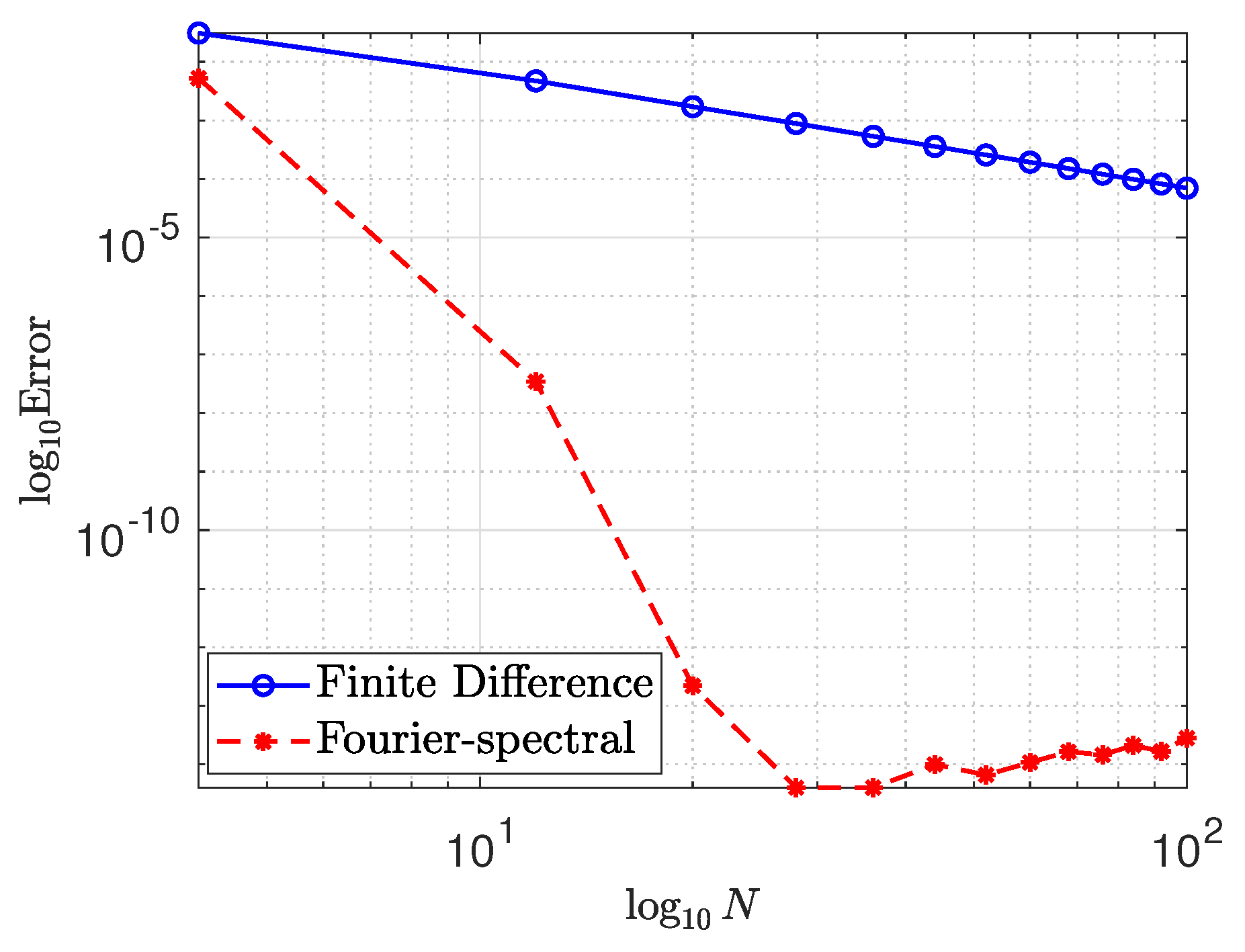
In this paper, we review the unconditionally gradient stable Fourier-spectral method for several phase-field equations. The phase-field models are derived from the variational approach that minimizes the free energy of the system. Thus, the derived system follows a law of energy dissipation, which configures thermodynamic consistency, and hence leads to a mathematically well-posed model. The spectral methods, which belong to the collection of weighted residual methods, are originally derived to solve the spatial part of partial differential equations. For detailed, rigorous, and numerical aspect information on spectral methods, see [1,2] and the references therein. In spectral methods, one usually takes a finite set of the expansion functions (so called trial or basis functions) to represent the numerical solution as a linear combination of those functions. Choosing the expansion parts is important because they form a basis for entire spectral domain. Furthermore, we implicitly assume that those functions are smooth, therefore the most common choices are orthogonal polynomials and trigonometric functions. Since our focus is the Fourier-spectral method, the trigonometric basis functions are regarded as the trial functions. Moreover, instead of regarding entire continuous space, the representation is imposed only at discrete points; this is why this method is so called pseudo-spectral method. It is enable to one can save the computing resources in evaluating differentiation and employ the efficient algorithm such as the fast Fourier transform when the number of grid points is even. In addition, the error is decreasing exponentially when one employs the Fourier-spectral method while the finite difference methods lead to the algebraically decreasing order in fact. Figure 1 shows the order of spectral accuracy compared with the order of accuracy of finite difference. In this case, we use a simple function ; hence . An error is defined as where is an approximation of .
According to Figure 1, the error is decreasing exponentially via Fourier-spectral method indeed. Furthermore, we verify the efficiency of the Fourier-spectral method employing the following initial-boundary value problem in one-dimensional space with the -periodic boundary condition.
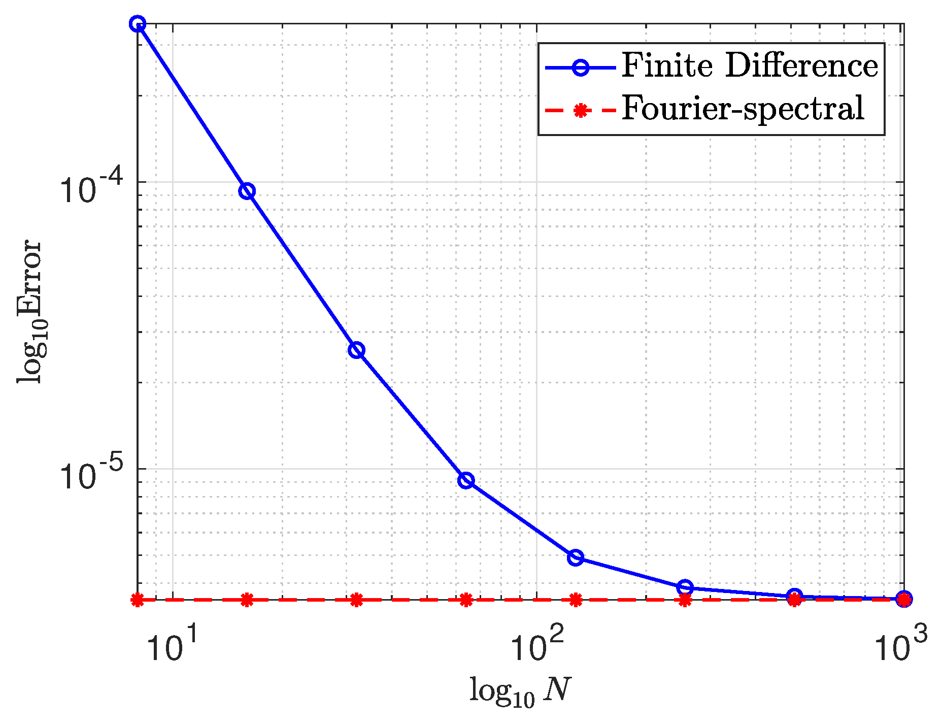
Then, the exact solution of Equation (1) is . Define as a numerical approximation to for where is a time step and is the number of iterations. Figure 2 depicts the convergence of second-order central finite difference scheme and Fourier-spectral method. Note that the backward difference method in time is employed to both cases and an error is defined as where N is the number of grid points, hence the number of modes, and it is easily verified that the Fourier-spectral method requires relatively few grid points within similar accuracy indeed.
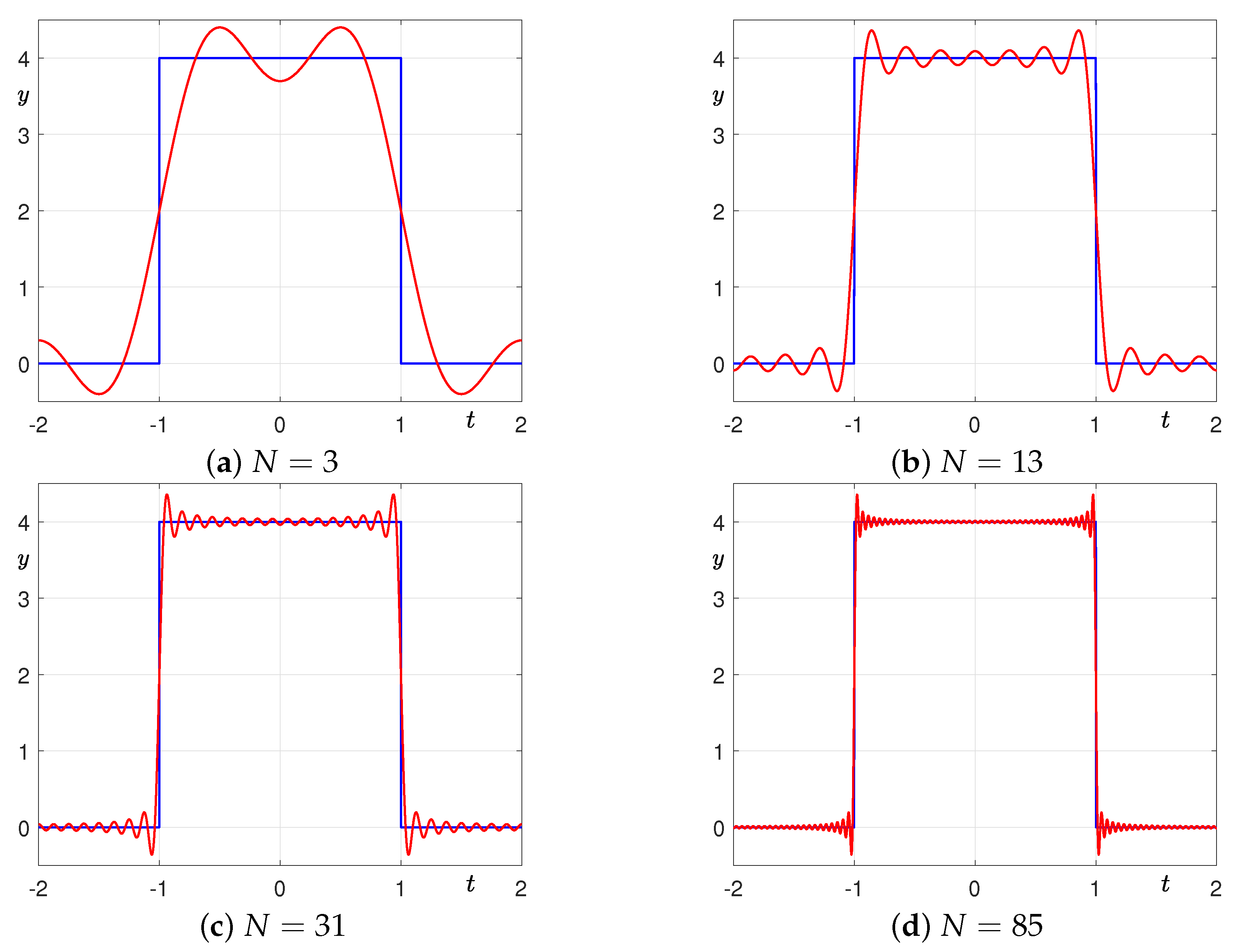
Sometimes, an interpolant cannot apply to less flexible domains since the method employs implicitly periodic or homogeneous boundary conditions though there is an advantage in numerical accuracy. Therefore, a somewhat subtle additional process is required to employ complex or mixed boundary conditions. Moreover, it causes Gibbs phenomenon if there is a point of discontinuity, i.e., when it has a sharp gradient. Figure 3 shows the oscillations near discontinuities when one employs the Fourier interpolant.
Moreover, we set all the mobility terms in phase-field models as constant for convenience, more precisely set to 1 without loss of generality, since it requires further manipulation to handle a variable mobility in spectral methods [3].
The Allen–Cahn (AC) equation is discussed first. It describes the temporal evolution of a non-conserved order field during anti-phase domain coarsening [4]:
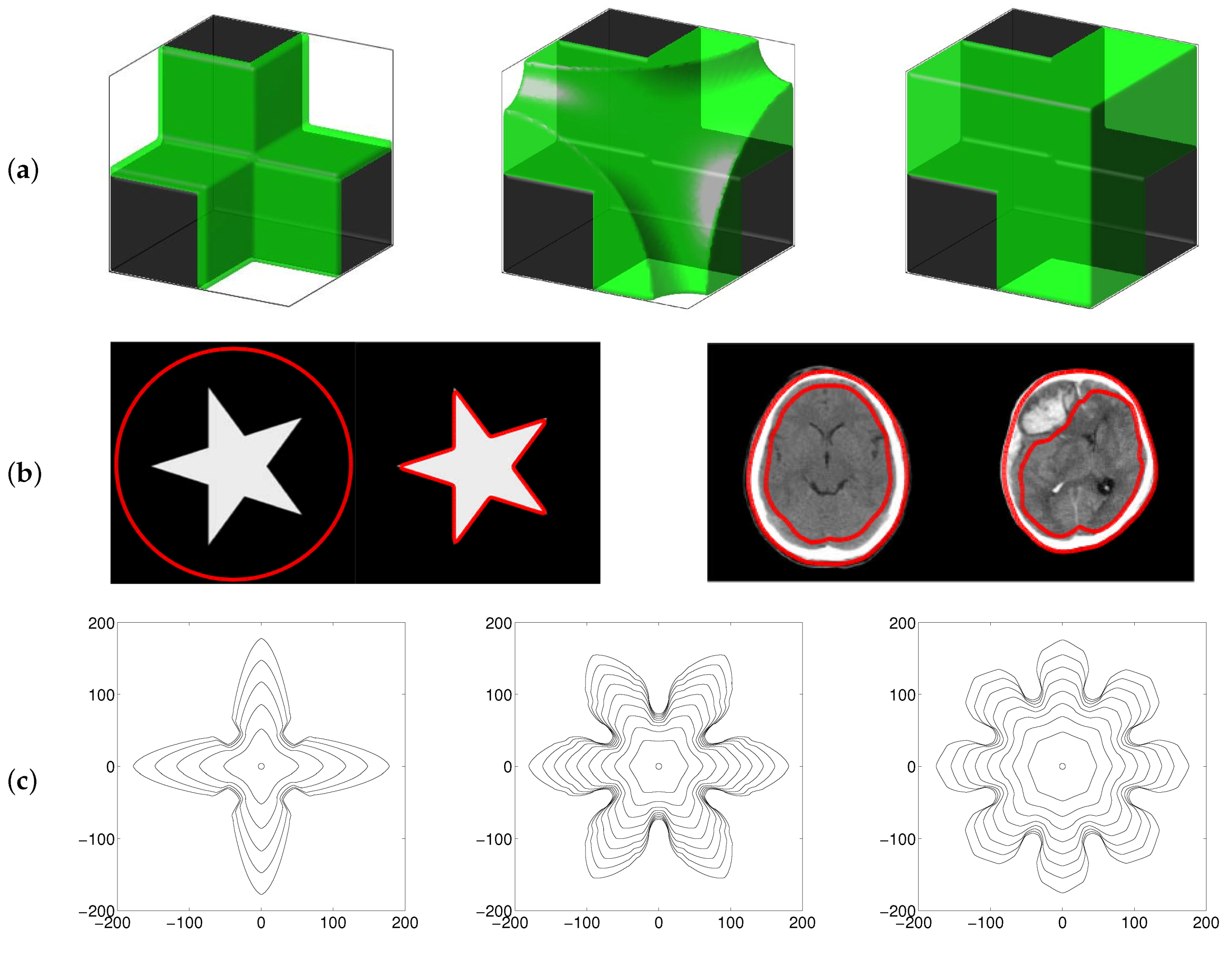
where is defined as the difference between the concentrations of the two components in a mixture, which varies on to 1, is the free energy potential, and is a small constant related to the interfacial energy. Note that . The AC equation has a wide range of applications such as mean curvature flows, two-phase incompressible fluids, complex dynamics of dendritic growth, image inpainting, and image segmentation, see Figure 4 for some of these examples [5,6,7].
Lee and Lee [8] presented unconditionally energy stable first- and second-order semi-analytical Fourier-spectral methods for the AC equation to reduce the errors caused by large time step. Those methods were originated by decomposition of original equation into two parts, linear and nonlinear, that have closed-form solutions; hence operator splitting steps ensure high-order nonlinear solvers.
The next is a similar type to the previous one, the Cahn–Hilliard (CH) equation, which models the process of spinodal decomposition in conserved binary alloys [9]:
The CH equation is widely used in applications such as phase separation, topology optimization, multiphase incompressible fluid flows, image inpainting, surface reconstruction, diblock copolymer, tumor growth simulation, and microstructures with elastic inhomogeneity, see Figure 5 for some of these examples [10].
Recently in [11], the discretization via nonlinear stabilized splitting scheme to the CH equation was reviewed and was solved by using a nonlinear multigrid method. Further in [12], Lee researched energy stability of the second-order strong-stability-preserving implicit-explicit Runge–Kutta methods for the CH equation. Christlieb et al. [13] presented the unconditionally gradient nonlinearly stabilized method for the CH equation, which is originally proposed by Eyre [14], within Fourier method and proposed an iterative scheme which is convergent for large time steps. There are a bunch of research related in AC and CH equations so far, some selected literatures are listed as follows. Montanelli and Bootland [15] proposed several exponential integration formula and compared their performance within stiff partial differential equations including AC and CH models. Such models are rewritten to sum of linear operator part with high-order terms and nonlinear operator part, and then Fourier-spectral method is applied in order to employ exponential integrator to this semilinear ordinary differential equations. Zhang and Liu [16] used several AC or CH type equations to represent the spatial patterns in ecological and biological system. Shen and Yang [17] presented numerical approximations of the AC and CH equations for semi-implicit or implicit schemes which are unconditionally energy stable, with stability analysis and error estimates based on spectral-Galerkin method. The results confirmed that spectral methods are suitable for diffusive interface models. Regarding on this respect especially, we introduce a nonlocal CH equation, which is appropriate to apply the Fourier-spectral method, that can model microphase separation in diblock copolymers, which consist of two different types of monomers [18] and an explicit form is listed as follows:
where is inversely proportional to the square of the total chain length of the copolymer and is the average concentration over the domain . Block copolymer is a linear-chain molecule consists of at least two subchains connected to each other to make a polymer chain. A diblock copolymer exists if the subchain consists of two distinct monomer blocks. Related mathematical models have been developed in order to investigate the behaviors of phase separation of block copolymers and to find an available technique to manufacture nano-structured materials [19,20,21,22]. There is a direct applications of Equation (4) in [23] recently, where the authors employ the spectral method and see the references therein to check more details.
The Swift–Hohenberg (SH) equation was originally derived to model patterns from the influence of thermal fluctuations in hydrodynamics [24]:
where is a density field and is a temperature related positive constant. There are several applications to employ this model such as cellular materials, metallurgy, laser dynamics, electrohydrodynamics, crystallography, etc. See [25,26,27,28] and the references therein for more details. In addition, we introduce a classical phase field crystal (PFC) equation which takes account for atomic-crystallization growth [29]:
This model has a variety of applications such as crystallization in liquid-liquid interface with undercooled material, isotropic phase separation, etc. On the atomistic/molecular scale freezing, a theoretical approach to undercooled liquids crystallization has been studied in [30,31], and the efficient numerical methods based on the operator splitting method or spectral method are developed for the phase-field crystal model [32,33]. The operator splitting method with Fourier-spectral method can relax the time step restriction or shorten the computation time depending on which a solver is applied for each stage.
A molecular beam epitaxy (MBE) growth model describes a process in which a thin single crystal layer is deposited on a single crystal substrate using molecular beams [34,35]:
The MBE model is a substantially used approach for thin-film deposition of a surface or interface quality determined to single-monolayer precision. This procedure is widely applied in semiconductor heterostructures and persistently studied topic in material science. Consequently, considerable mathematical models have been evolved to study the epitaxy dynamics, covering from continuum models to molecular dynamical simulations. The readers are referred to the following references for more details [36,37,38,39,40,41,42,43].
The main purpose of this paper is to present brief reviews, to describe numerical solution algorithms, and to provide the MATLAB code implementations of the unconditionally gradient stable Fourier-spectral method for the several phase-field equations. In particular, we highlight the caution that needs to be taken when applying the MATLAB based fast Fourier transform to the Fourier-spectral method.
The outline of this paper is as follows. The numerical solutions in two- and three-dimensional cases of the above phase-field models are described in Section 2 and Section 4, respectively. In Section 3 and Section 5, we present the basic numerical simulations to the stated phase-field models in both two- and three-dimensional cases. We finalize the paper with the conclusion in Section 6. In the Appendix A, we provide the MATLAB codes for the numerical implementation of the presented equations.
2. Numerical Solutions in 2D
In this section, we present unconditionally stable Fourier-spectral methods for the phase-field models in two-dimensional space . Let , be positive even integers and , be the length of each direction, respectively; hence define and as the spatial step size in each direction, respectively. We denote discretized points as where and are integers. Let be an approximation of , where and is the temporal step size. For the given data and , the discrete Fourier transform is defined as
where and . The inverse discrete Fourier transform is
Note that we can obtain spectral derivatives as if we perform analytic differentiations in the Fourier space. We assume that is sufficiently smooth and extended to continuous version of the numerical approximation . The following shows step-by-step description of how the differentiation works in the Fourier transform with finite basis.
This process enables one can derive spectral derivatives in the Fourier space easily, not differentiate directly in the physical space. Therefore, we can represent the Laplacian to coefficients in the Fourier space as follows:
where the first line is the definition of the inverse Fourier transform and the second line is just applying Equation (10) twice to x- and y-direction to and its Fourier transform.
Now we present the numerical solutions of phase-field equations. First, we derive the numerical solution of the AC equation. We apply the linearly stabilized splitting scheme [14] to Equation (2).
where . Thus, Equation (12) can be transformed into the discrete Fourier space as follows:
Therefore, we obtain the following discrete Fourier transform
Then, the updated numerical solution can be computed using Equation (9):
Next, we obtain the numerical solution of the CH equation. We employ the linearly stabilized splitting scheme [14] to Equation (3).
Thus, Equation (16) can be transformed into the discrete Fourier space as follows:
Therefore, we obtain the following discrete Fourier transform
Then, the updated numerical solution can be computed using Equation (9):
Now, we present a numerical solution to the SH equation. In a similar manner, we discretize Equation (5) as follows:
where . Then we transform Equation (20) as
Therefore, we have the following result
and hence we have a numerical solution as follows:
Similarly, a numerical solution for the PFC model (6) is obtained by the same procedure
Then Equation (24) is transformed as
Therefore, we have the following result
Subsequently, we have a numerical solution as follows:
The remaining one is a numerical solution to the MBE growth model (7). Discretize Equation (7) with an expanded divergence term and treat this in implicit way,
Note that and represent the discrete Fourier transform and the discrete inverse Fourier transform, respectively. Therefore, we have the following result
and then we update a numerical solution as follows:
3. Numerical Experiments in 2D
We perform several numerical investigations in this section. Note that we employ the -periodic boundary condition for overall numerical simulations in two-dimensional case. Sometimes, we employ the initial conditions as random perturbations in domain since these are adequate to reaction-diffusion type models. For AC and CH equations, since there are equilibrium solutions in one-dimensional space as hyperbolic tangent profiles on infinite domain, we use those as initial conditions. Furthermore, we take the value of model parameter as an approximate value close to , which is used in finite difference methods [44].
3.1. The AC Equation
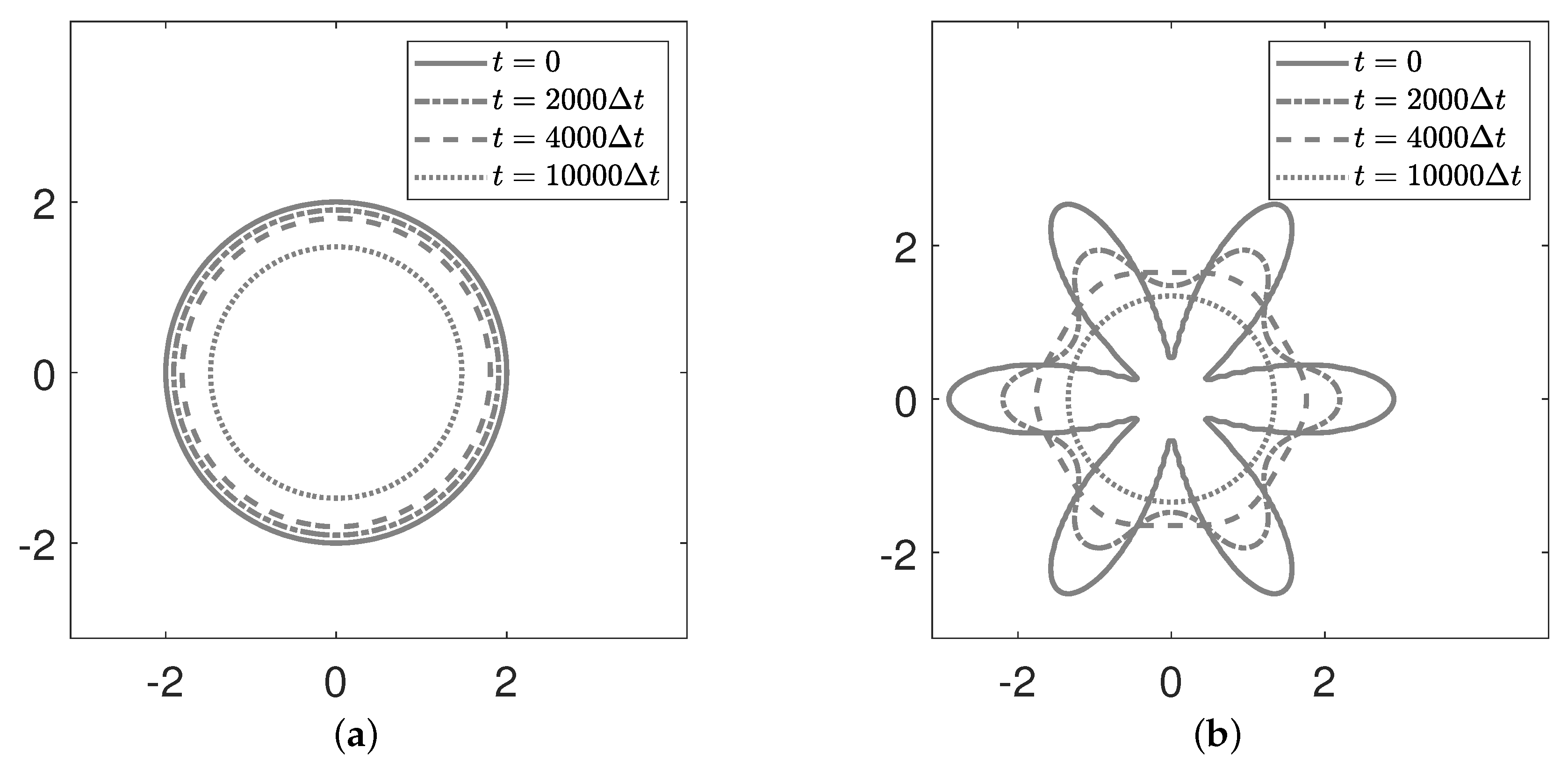
Numerical simulations are conducted to verify the mean curvature flow of the AC equation at first. Initial conditions are given as follows:
where for . Figure 6 shows the numerical test results at to the AC equation using the Fourier-spectral method. Here, we use , , , and . The final time is . The results reflect the motion by mean curvature characteristic of the AC equation.
3.2. The CH Equation
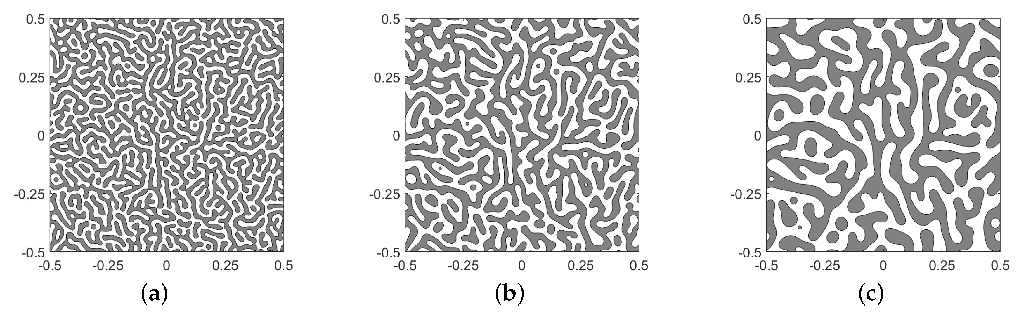
Next, we investigate the coarsening dynamics of the CH Equation (3) numerically with the following initial conditions,
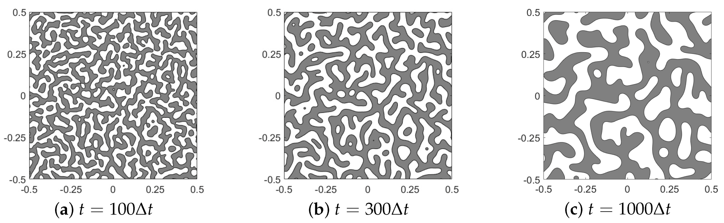
where rand denotes a random number between to 1 and . Figure 9 shows the numerical results at . We use , , , and . The results represent well the coarsening dynamics of the CH equation.
Figure 10 shows the numerical simulation results at to the CH equation with the initial condition (40). Here, , , , and are used.
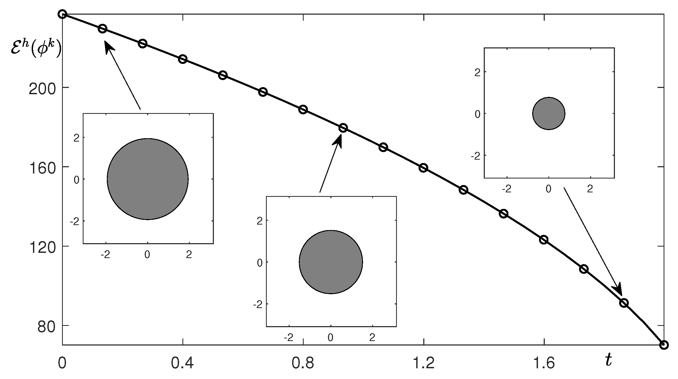
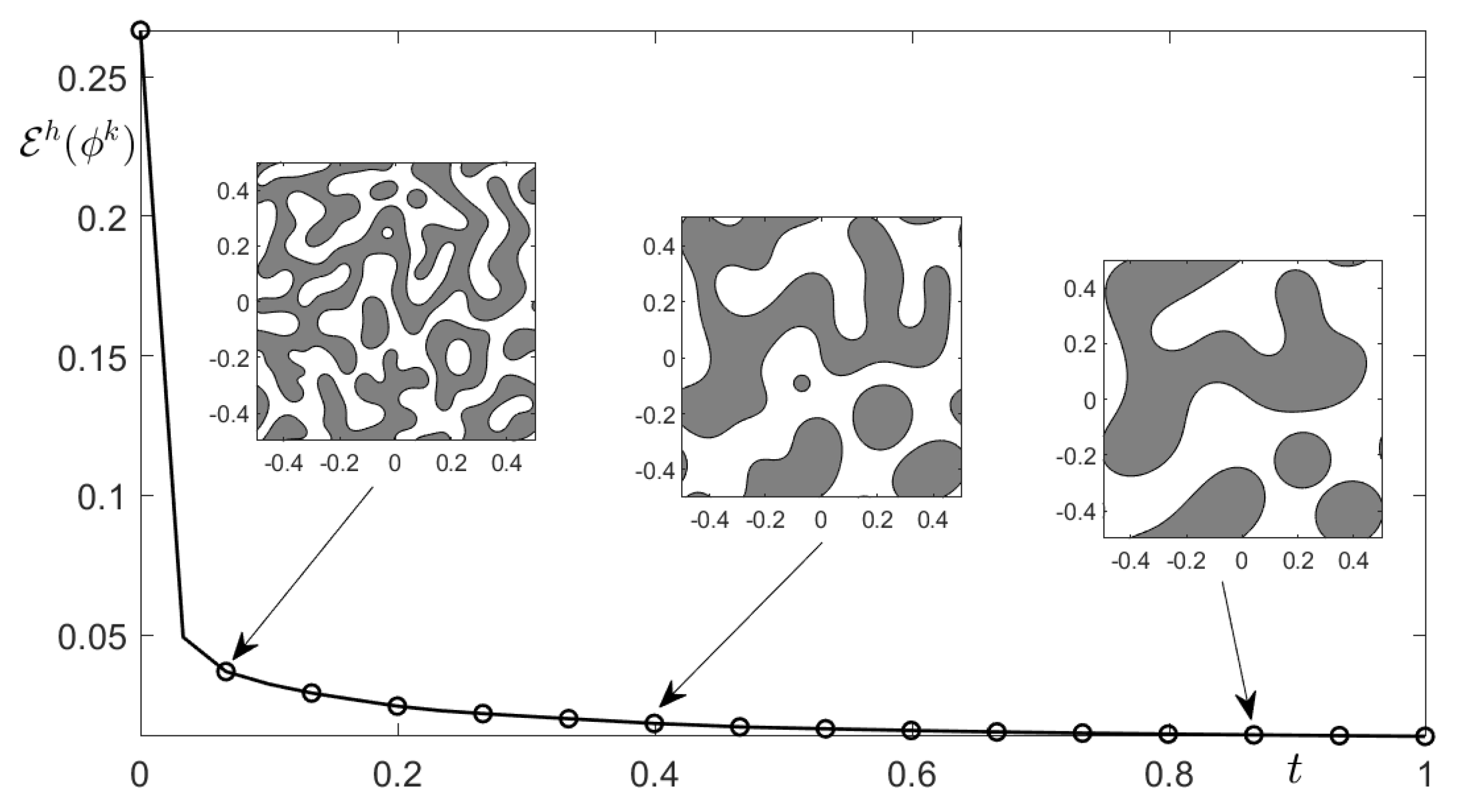
Furthermore, an energy dissipation of the CH equation is illustrated in Figure 11. We define a total free energy as follows:
We adopt the initial condition (39) and .
Further we present the phase separation behavior via nonlocal CH model for diblock copolymers. An initial condition is given by
A computational domain is given as . Here, we use , , , , , and . The final time is . Figure 12 shows the phase separation behaviors called the hexagonal patterns over time.
Another initial condition is given as follows:
A computational domain is given as . Parameter values are set to , , , , , and . The final time is . Figure 13 describes the phase separation behaviors called the lamellar patterns over time.
Consequently, we illustrate an energy dissipation of the nonlocal CH model (4). A total free energy is given by
where is obtained by solving . Now Equation (45) is discretized as
by using Equation (38). Figure 14 shows the energy dissipation of the nonlocal CH equation with the discrete energy (46). We employ the same condition in Figure 12 except for and .
3.3. The SH Equation
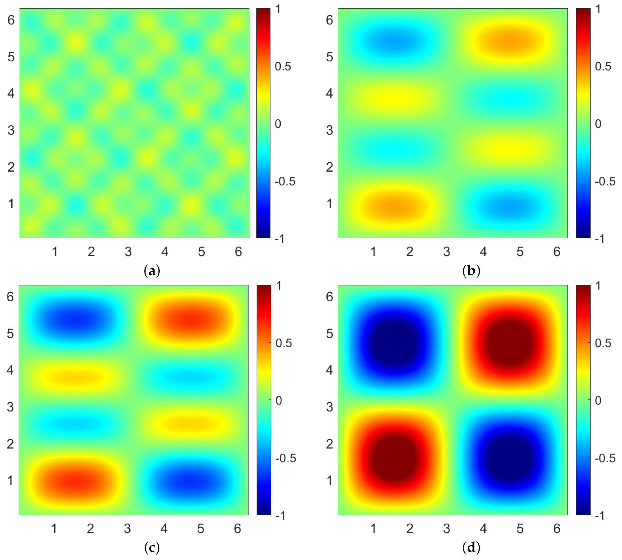
We present the pattern formation due to the SH Equation (5) in the rectangular domain . The initial condition is given as follows:
where . Here, we choose parameter values as , , , and . The final time is . Figure 15 depicts the pattern formation via instability of thermal fluctuations. Note that we fix the range of colors in .
For the next step, we investigate an energy decay of the following functional
3.4. Classical PFC Model
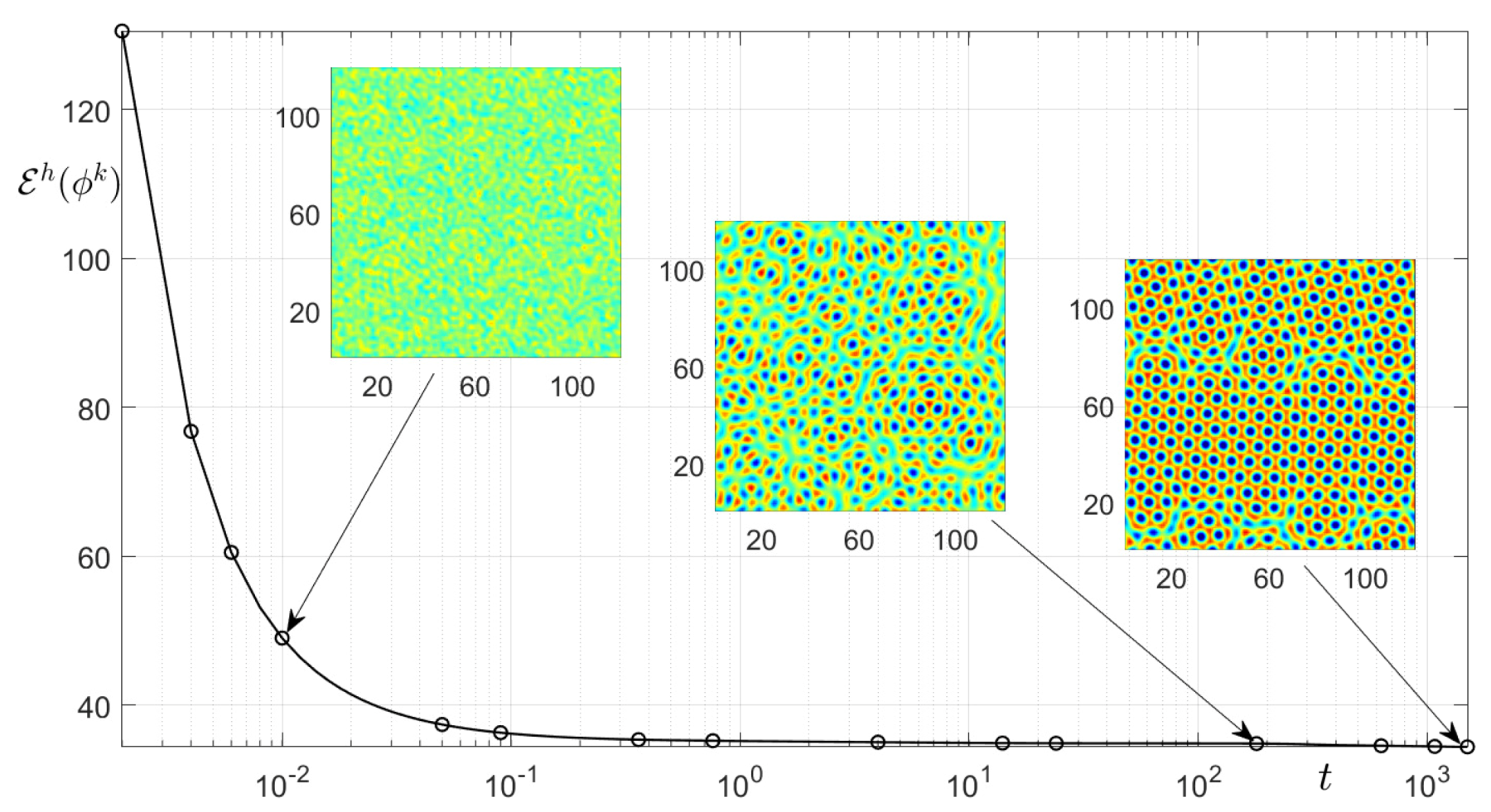
The phase separation behavior of the classical PFC model is described in this section. Numerical simulation is conducted in the rectangular domain . The initial condition is given as follows:
where . Parameters used here are , , , and . The final time is . Figure 17 illustrates the isotropic phase transition behaviors. Note that we restrict the range of colors in .
3.5. MBE Growth Model
The epitaxial growth of isotropic current MBE growth model is investigated in this section. Numerical simulation is conducted in the rectangular domain . The initial condition is given as follows:
Parameters are used as , , and . The final time is . Figure 19 illustrates the epitaxial growth in computational domain.
Further, we present an energy decay to the MBE growth model (7). An energy functional is given by
3.6. Logarithmic Free Energy
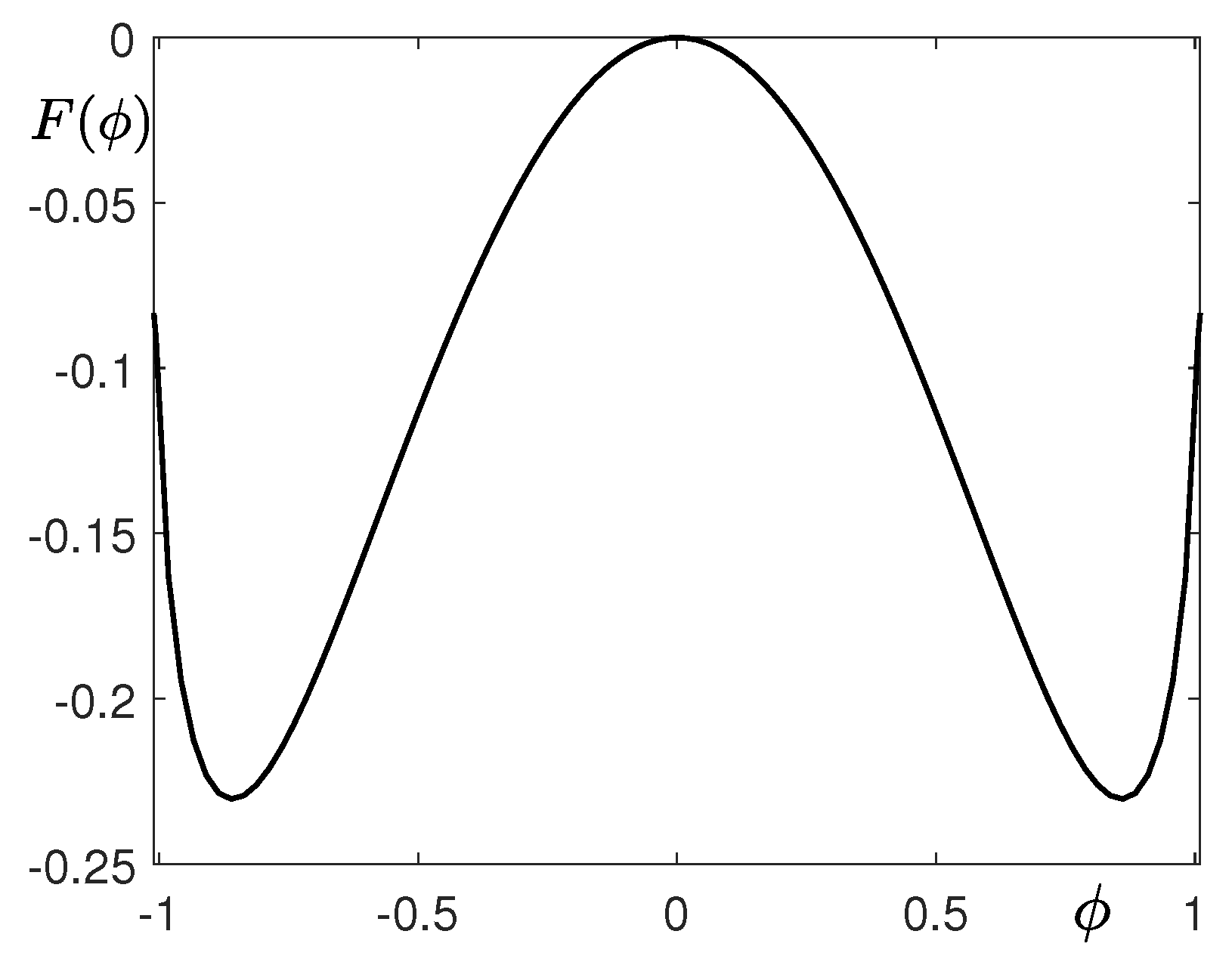
In this paper, we have used the polynomial form of double-well potential . Note that it is not the only choice. Now, we consider the logarithmic Flory–Huggins free energy [45,46]
for the AC and CH equations. Here, and is a positive constant, which are taken as 1 and 1.5, respectively, in this paper. Figure 21 illustrates the logarithmic free energy.
To solve the AC and CH equations with the logarithmic free energy (55), we also apply Eyre’s linearly stabilized splitting scheme [14]. First, we discretize the AC Equation (2) with a free energy (55):
where , and is an auxiliary constant for the splitting scheme [47]. Then, Equation (56) can be transformed into the discrete Fourier space as follows:
Therefore, we obtain the following discrete Fourier transform
Then, the updated numerical solution can be computed using Equation (9):
We conduct a numerical test with the following initial condition is
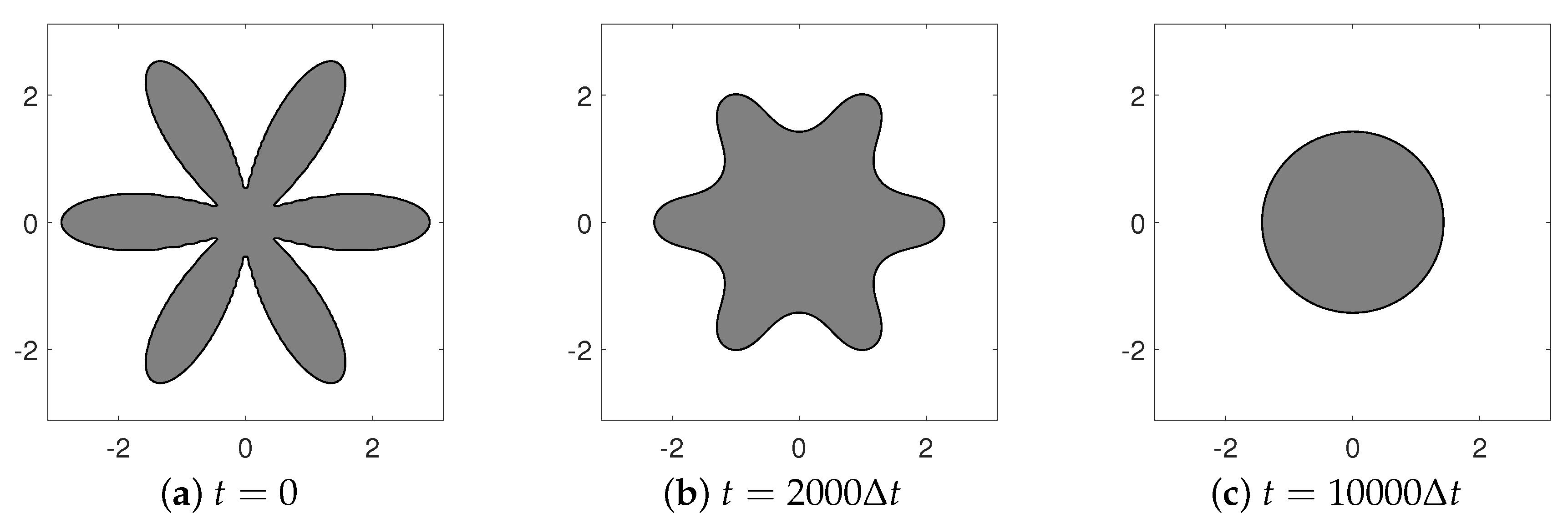
where for . We set the parameters as and . Figure 22 shows the zero-level contours over time with the initial condition (60) according to motion by mean curvature.
Next, we obtain the numerical solution of the CH Equation (3) with the logarithmic free energy (55). Applying the linearly stabilized splitting scheme [14] to the governing equation, we get
Thus, Equation (61) can be transformed into the discrete Fourier space as follows:
Therefore, we obtain the following discrete Fourier transform
Then, the updated numerical solution can be computed using Equation (9):
We perform the numerical test to the CH equation with the following initial condition (39) on the computational domain . We use , , , and . Figure 23a–c shows the numerical results at and , respectively, and represent well the coarsening dynamics of the CH equation.
According to the numerical simulation results, the unconditionally stable Fourier-spectral method ensures the fast convergence that error is decaying exponentially since the collocation points in physical space guarantee the exact function values in the Fourier space and the method provides a sufficiently smooth basis function (an exponential basis function in this case), one can obtain high-order approximations of derivatives. Moreover, it has almost linearly increasing calculation speed when a large number of grid points are used; hence one can represent the spatial details of numerical results with sufficient grid points in a short time.
4. Numerical Solutions in 3D
We extend the Fourier-spectral method on two-dimensional space to three-dimensional space, for the stated phase-field models. Let , , be positive even integers and , , be the length of each direction, respectively. We denote discretized points by for , , , where , , is the spatial step size in each direction, respectively. For , is denoted by , where is the temporal step. For the given data , , , the discrete Fourier transform is defined as
where , , . The inverse discrete Fourier transform is
Similar to the two-dimensional case, we assume that is sufficiently smooth and extended to continuous version of the numerical approximation . Therefore, we can obtain the following result.
Consequently, we can write Laplacian as coefficients in the Fourier space as follows:
where the first line is the definition of the inverse Fourier transform and the second line is just applying Equation (67) twice to x-, y-, and z-direction to and its Fourier transform. Now, we present the numerical solutions of three-dimensional phase-field models. Since most of the calculations are redundant, we just briefly list as follows by extending the solvers in two-dimensional space to those of three-dimensional space. Note that the functions f and g which are defined in Section 2 are simply extended to three-dimensional domain. The following is a numerical solution to the AC Equation (2).
Then, the renewed numerical solution can be computed using Equation (66):
Next one is a numerical solution to the CH Equation (3).
Then, the renewed numerical solution can be calculated using Equation (66):
The following is a numerical solution to the SH Equation (5).
and hence we have a numerical solution as follows:
Subsequently, we have a numerical solution to the classical PFC model (6) as follows.
Therefore, we have a numerical solution as follows:
5. Numerical Experiments in 3D
5.1. The AC Equation
We perform the numerical test to the AC Equation (2) with the following initial condition,
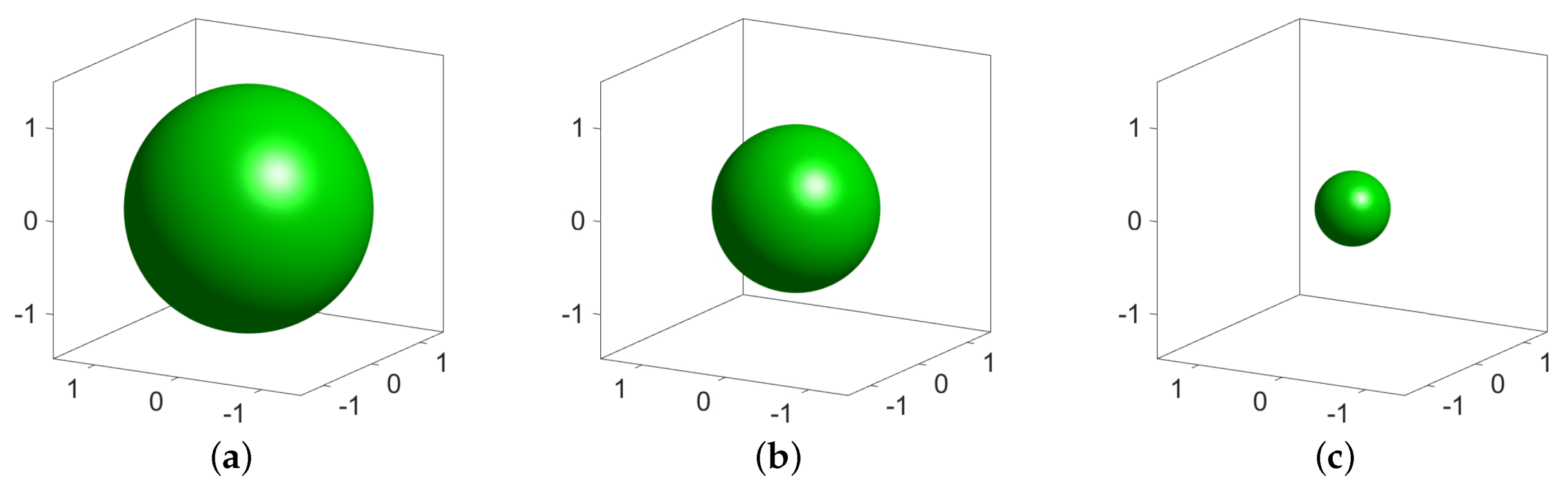
Figure 24 shows the numerical solutions at to the 3D AC equation using the Fourier-spectral method for . Here, we use , , , and . The final time is . Similar to the two-dimensional case, the simulation results depict the motion by mean curvature property quite well.
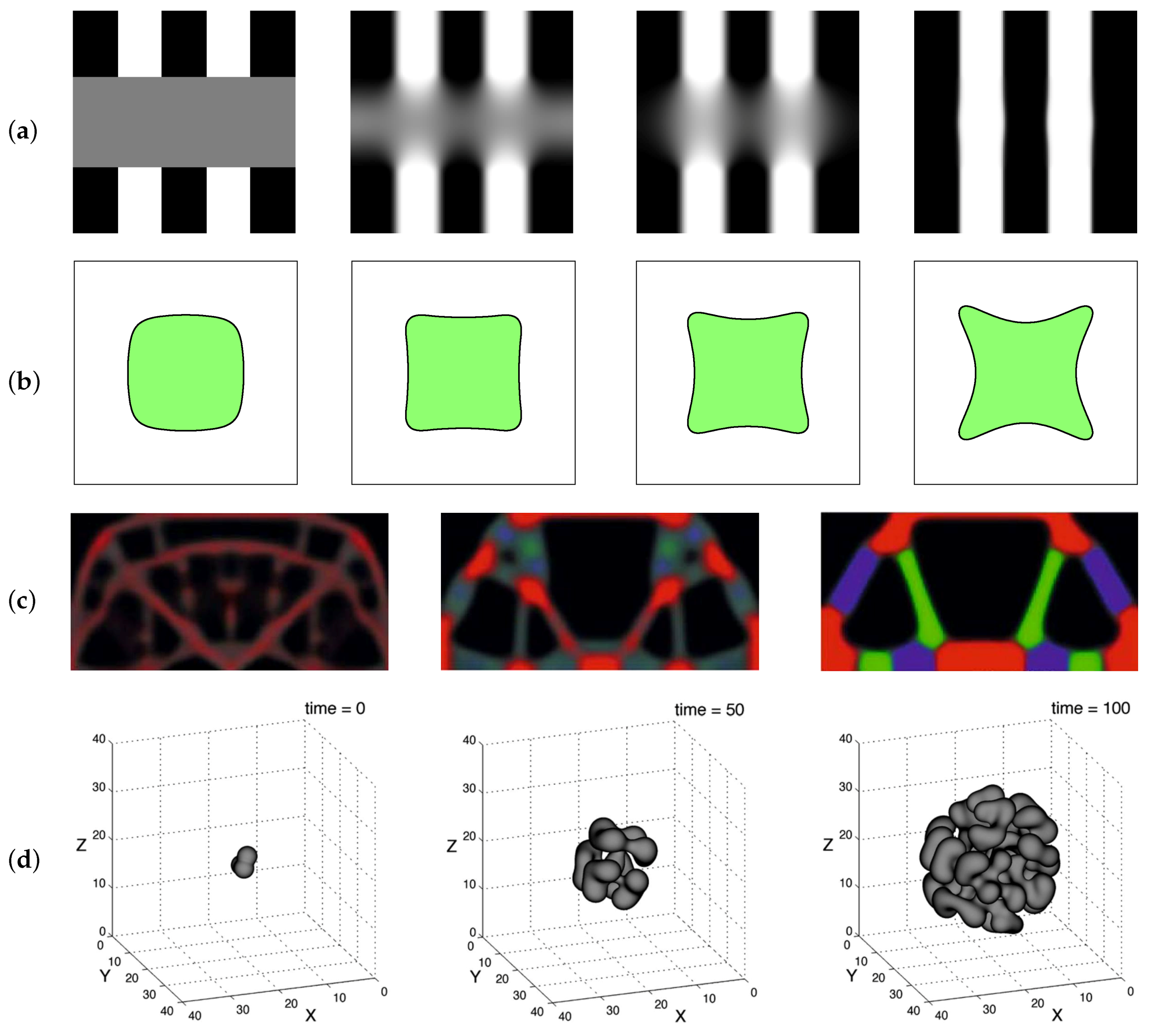
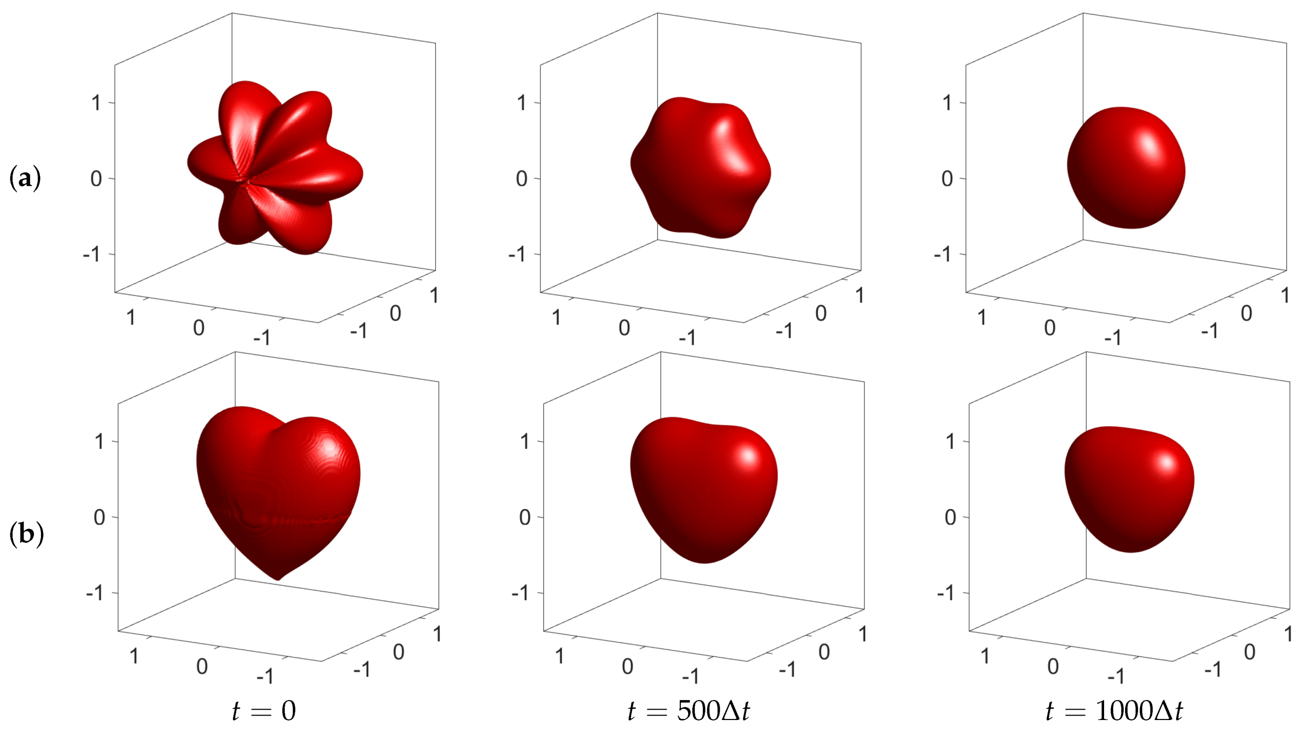
We performed the numerical experiment for the complex shape to the 3D AC equation. We defined two initial conditions of complex shape as the following:
where for . Figure 25 shows the numerical test results at . Here, we use , , , and .
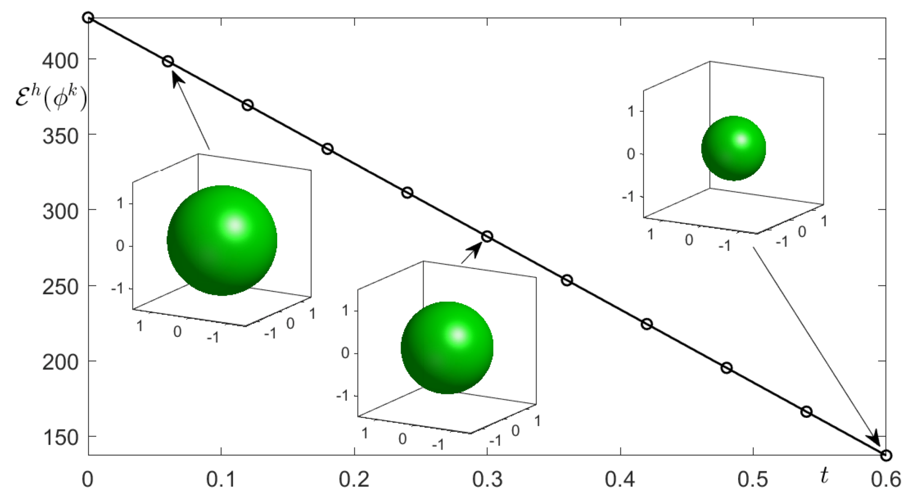
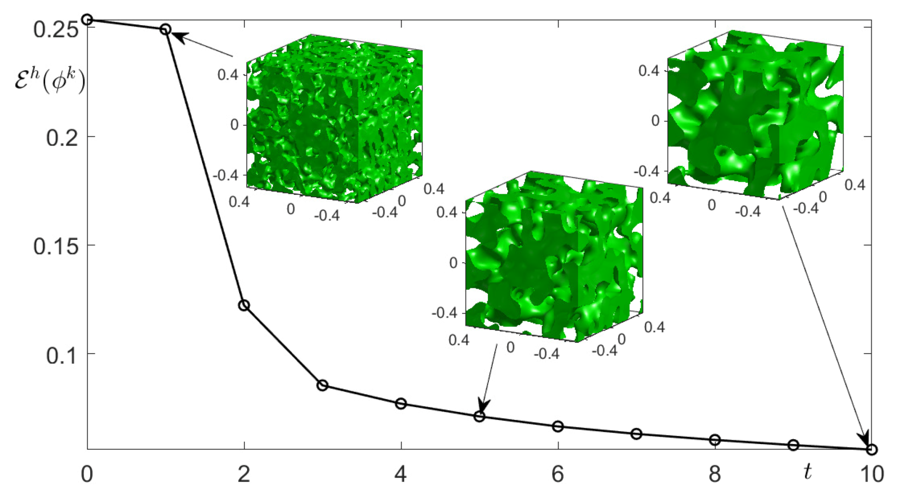
Furthermore, we present the energy dissipation to the AC equation in three-dimensional space. The discrete energy has a form as follows:
5.2. The CH Equation
Next, we investigated the numerical test to the CH Equation (3) with the following initial conditions,
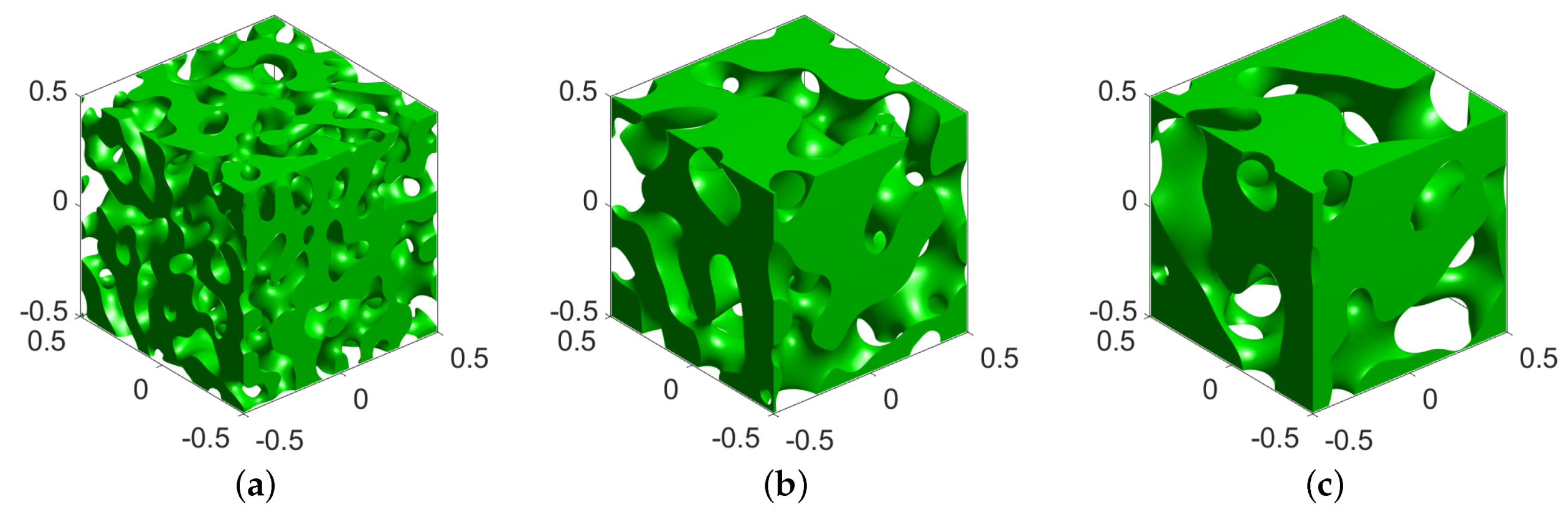
where rand implies a random number generating function ranged from to 1 and . Figure 27 shows the numerical investigation results at , and to the 3D CH equation using the Fourier-spectral method with the initial condition (81). Here, we use , , , and .
Figure 28 depicts the numerical simulation results to the 3D CH equation using the Fourier-spectral method with the initial condition (82). Here, we use , , , and . The above results represent well the coarsening dynamics of the CH equation. Moreover, we present the energy dissipation to the CH equation in three-dimensional space. We extend Equation (42) to three-dimensional case as follows:
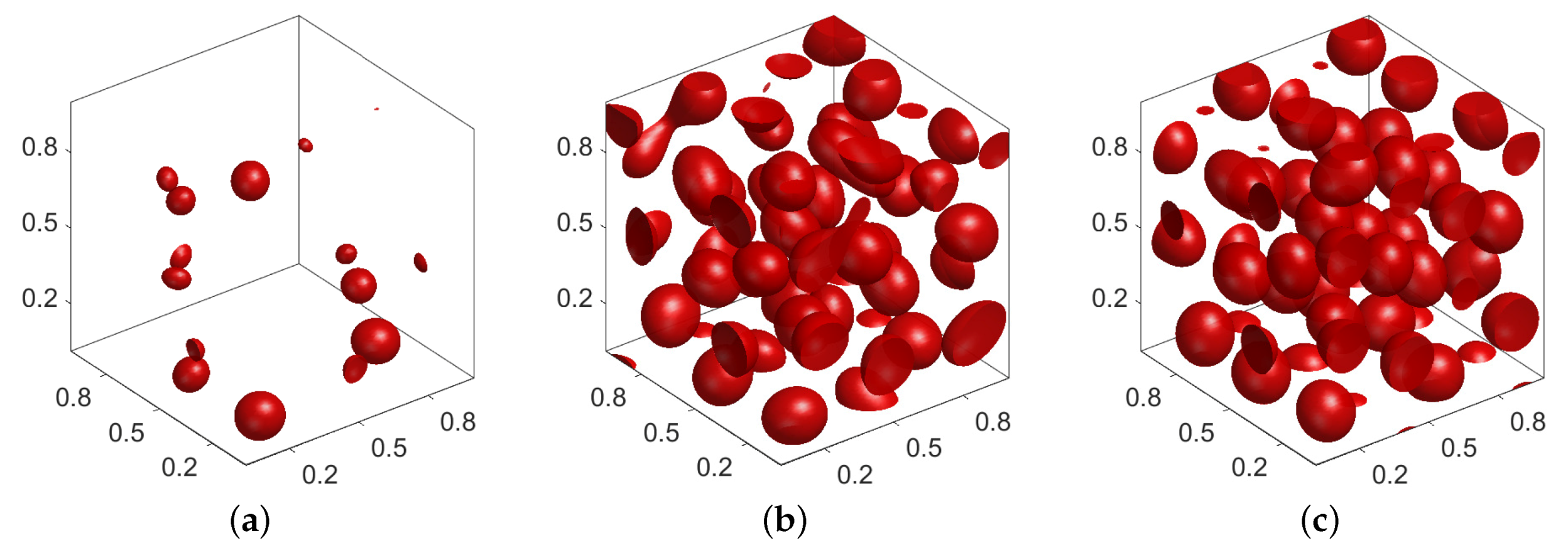
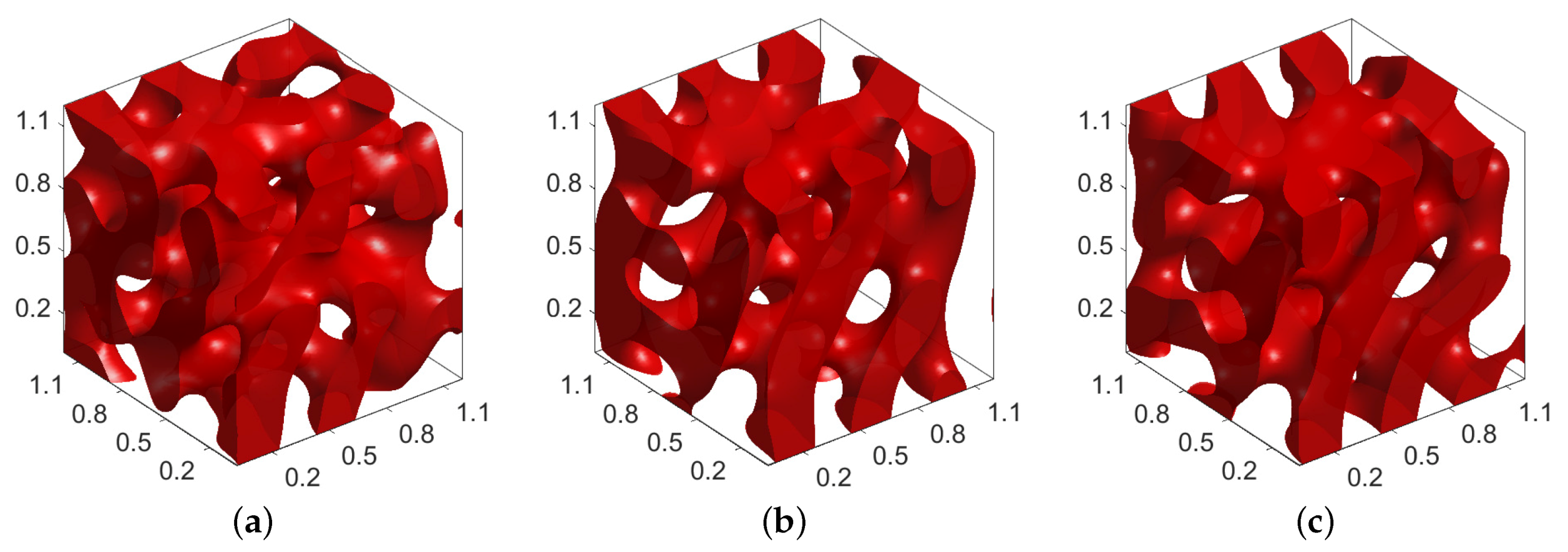
Further we present phase separation behaviors of the nonlocal CH equation in the domain . An initial condition is given by
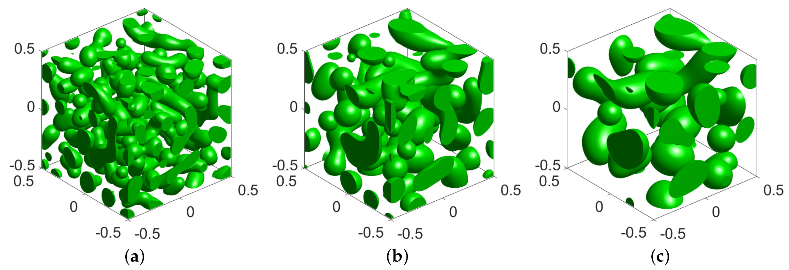
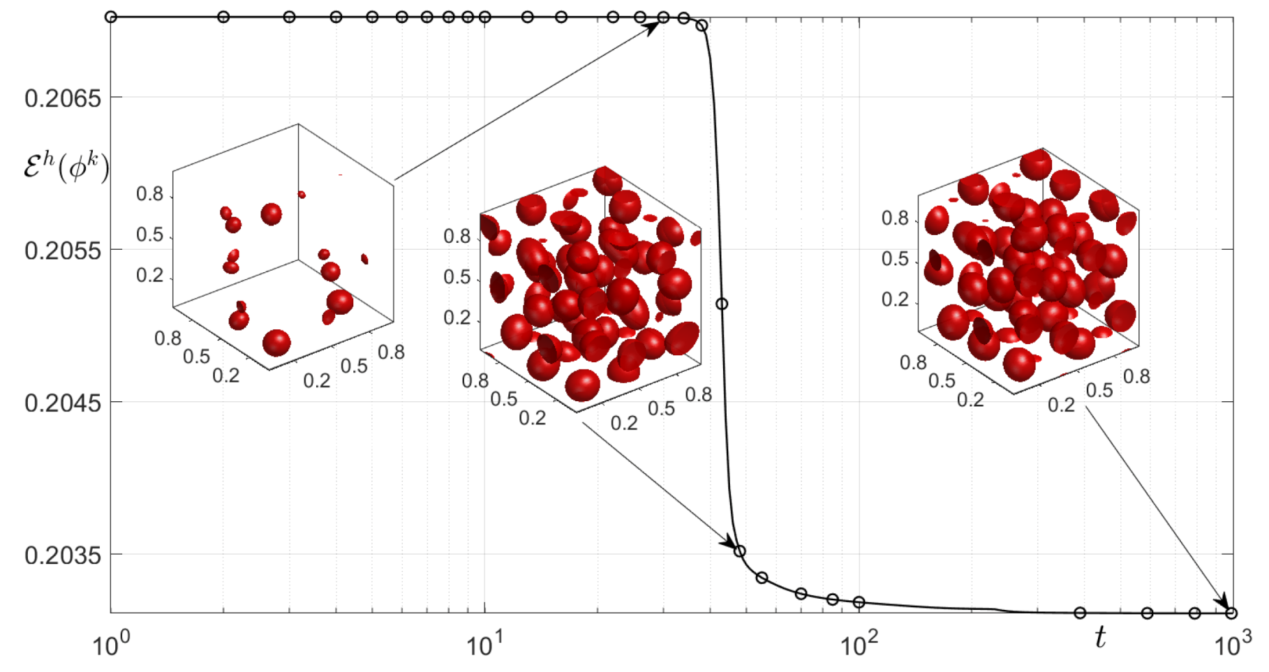
Figure 30 shows the snapshots of the spherical pattern formation via nonlocal CH equation. Here, we use Equation (84) with , , , , , and . The final time is .
5.3. The SH Equation
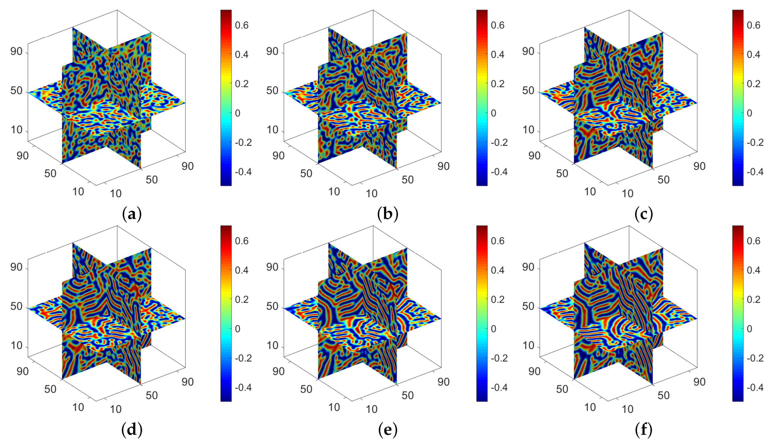
We present numerical simulation results to the SH equation in this section. A computational domain is . An initial condition is given as
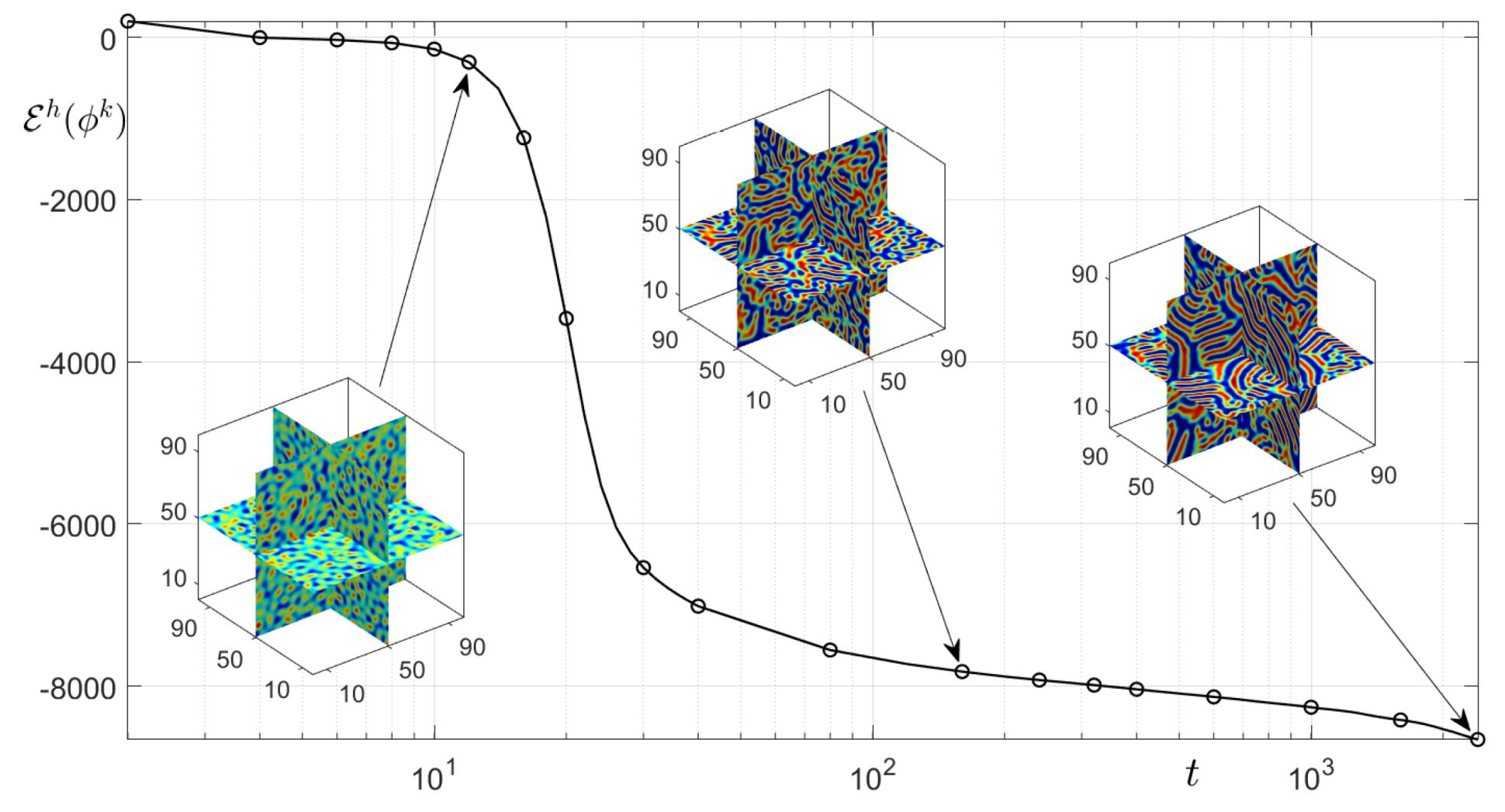
where . Figure 33 shows the patterns due to the instability of thermal fluctuations. Here, we use , , , and . The final time is .
5.4. Classical PFC Model
We present numerical simulation results to the classical PFC model in the three-dimensional domain . An initial condition is given as
where . Figure 35 shows the phase transition behaviors of this PFC model. Here, we use , , , and . The final time is .
6. Conclusions
In this paper, we briefly investigate the Fourier-spectral method to the phase-field equations in two- and three-dimensional cases, especially focused on AC, CH, SH, PFC, MBE growth models which are very important parabolic partial differential equations and are applicable to a lot of interesting scientific problems. We present detailed descriptions and numerical solutions of the unconditionally gradient stable Fourier-spectral method and explain its connection to MATLAB usage so that the interested readers can simply implement the corresponding Fourier-spectral method for their research needs without difficulties. Numerical simulation results yield the corresponding method represents well the characteristics of each equation. Furthermore, we provide the MATLAB codes for these equations in the Appendix A.
Author Contributions
All the authors contributed as follows. Conceptualization, J.K.; methodology, S.Y., D.J. and H.G.L.; software, S.Y., C.L., H.K. and S.K.; validation, S.Y., D.J., C.L. and J.K.; formal analysis, S.Y. and D.J.; investigation, S.Y., C.L., H.K., S.K. and J.K.; resources, D.J.; data curation, S.Y., H.K. and S.K.; writing—original draft preparation, S.Y., D.J., C.L., H.K., S.K. and J.K.; writing—review and editing, S.Y., C.L., H.G.L. and J.K.; visualization, S.Y., C.L., H.K. and S.K.; supervision, D.J. and J.K.; project administration, J.K.; funding acquisition, S.Y., D.J., C.L., H.K., H.G.L. and J.K. All authors have read and agreed to the published version of the manuscript.
Funding
The first author (S.Y.) was supported by the Brain Korea 21 Plus (BK 21) from the Ministry of Education. The author (D.J.) was supported by the National Research Foundation of Korea (NRF) grant funded by the Korea government (MSIP) (NRF-2017R1E1A1A03070953). The author (C.L.) was supported by Basic Science Research Program through the National Research Foundation of Korea (NRF) funded by the Ministry of Education (NRF-2019R1A6A3A13094308). The author (H.K.) was supported by Basic Science Research Program through the National Research Foundation of Korea (NRF) funded by the Ministry of Education (NRF-2020R1A6A3A13077105). The author (H.L.) was supported by the National Research Foundation of Korea (NRF) grant funded by the Korea government (MSIT) (No.2019R1C1C1011112). The corresponding author (J.K.) was supported by Basic Science Research Program through the National Research Foundation of Korea (NRF) funded by the Ministry of Education (NRF-2019R1A2C1003053).
Acknowledgments
The authors thank the reviewers for the constructive and helpful comments on the revision of this article.
Conflicts of Interest
The authors declare no conflict of interest.
Appendix A
The following MATLAB codes are available from the corresponding author’s webpage: http://elie.korea.ac.kr/~cfdkim/codes/.
Appendix A.1. The AC Equation in 2D
| clear; |
| Nx=128; Ny=128; Lx=2*pi; Ly=2*pi; hx=Lx/Nx; hy=Ly/Ny; |
| x=linspace(−0.5*Lx+hx,0.5*Lx,Nx); |
| y=linspace(−0.5*Ly+hy,0.5*Ly,Ny); |
| [xx,yy]=ndgrid(x,y); epsilon=0.05; Cahn=epsilon^2; |
| u=tanh((2-sqrt(xx.^2+yy.^2))/(sqrt(2)*epsilon)); |
| p=2*pi/Lx*[0:Nx/2 -Nx/2+1:−1]; |
| q=2*pi/Ly*[0:Ny/2 -Ny/2+1:−1]; |
| p2=p.^2; q2=q.^2; [pp2,qq2]=ndgrid(p2,q2); |
| dt=0.01; T=3; Nt=round(T/dt); ns=Nt/20; |
| figure(1); clf; |
| contourf(x,y,real(u’),[0 0]); axis image |
| axis([x(1) x(Nx) y(1) y(Ny)]) |
| pause(0.01) |
| for iter=1:Nt |
| u=real(u); |
| s_hat=fft2(Cahn*u-dt*(u.^3-3*u)); |
| v_hat=s_hat./(Cahn+dt*(2+Cahn*(pp2+qq2))); |
| u=ifft2(v_hat); |
| if (mod(iter,ns)==0) |
| contourf(x,y,real(u’),[0 0]); |
| axis image |
| axis([x(1) x(Nx) y(1) y(Ny)]) |
| pause(0.01) |
| end |
| end |
Appendix A.2. The AC Equation in 3D
| clear; |
| Nx=128; Ny=128; Nz=128; Lx=1.2; Ly=1.2; Lz=1.2; hx=Lx/Nx; hy=Ly/Ny; hz=Lz/Nz; |
| x=linspace(−0.5*Lx+hx,0.5*Lx,Nx); |
| y=linspace(−0.5*Ly+hy,0.5*Ly,Ny); |
| z=linspace(−0.5*Lz+hz,0.5*Lz,Nz); |
| [xx,yy,zz]=ndgrid(x,y,z); epsilon=hx; Cahn=epsilon^2; |
| u=rand(Nx,Ny,Nz)−0.5; |
| kx=2*pi/Lx*[0:Nx/2 -Nx/2+1:−1]; |
| ky=2*pi/Ly*[0:Ny/2 -Ny/2+1:−1]; |
| kz=2*pi/Lz*[0:Nz/2 -Nz/2+1:−1]; |
| k2x = kx.^2; k2y = ky.^2; k2z = kz.^2; |
| [kxx,kyy,kzz]=ndgrid(k2x,k2y,k2z); |
| dt=0.01; T=0.5; Nt=round(T/dt); ns=Nt/10; |
| for iter=1:Nt |
| u=real(u); |
| s_hat=fftn(Cahn*u-dt*(u.^3-3*u)); |
| v_hat=s_hat./(Cahn+dt*(2+Cahn*(kxx+kyy+kzz))); |
| u=ifftn(v_hat); |
| if (mod(iter,ns)==0) |
| figure(1); clf; |
| p1=patch(isosurface(xx,yy,zz,real(u),0.)); |
| set(p1,‘FaceColor’,‘g’,‘EdgeColor’,‘none’); daspect([1 1 1]) |
| camlight;lighting phong; box on; axis image; |
| view(45,45); |
| pause(0.01) |
| end |
| end |
Appendix A.3. The CH Equation in 2D
| clear; |
| Nx=150; Ny=150; Lx=1; Ly=1; hx=Lx/Nx; hy=Ly/Ny; |
| x=linspace(−0.5*Lx+hx,0.5*Lx,Nx); |
| y=linspace(−0.5*Ly+hy,0.5*Ly,Ny); |
| epsilon=0.0125; Cahn=epsilon^2; |
| u=0.05*(2*rand(Nx,Ny)−1); |
| p=2*pi/Lx*[0:Nx/2 -Nx/2+1:−1]; |
| q=2*pi/Ly*[0:Ny/2 -Ny/2+1:−1]; |
| p2=p.^2; q2=q.^2; [pp2,qq2]=ndgrid(p2,q2); |
| dt=0.01; T=0.5; Nt=round(T/dt); ns=Nt/50; |
| figure(1); clf; |
| contourf(x,y,real(u’),[0 0]); axis image |
| axis([x(1) x(Nx) y(1) y(Ny)]) |
| pause(0.01) |
| for iter=1:Nt |
| u=real(u); |
| s_hat=fft2(u)-dt*(pp2+qq2).*fft2(u.^3-3*u); |
| v_hat=s_hat./(1.0+dt*(2.0*(pp2+qq2)+Cahn*(pp2+qq2).^2)); |
| u=ifft2(v_hat); |
| if (mod(iter,ns)==0) |
| contourf(x,y,real(u’),[0 0]); |
| axis image |
| axis([x(1) x(Nx) y(1) y(Ny)]) |
| pause(0.01) |
| end |
| end |
Appendix A.4. The CH Equation in 3D
| clear; |
| Nx=128; Ny=128; Nz=128; Lx=1.2; Ly=1.2; Lz=1.2; hx=Lx/Nx; hy=Ly/Ny; hz=Lz/Nz; |
| x=linspace(−0.5*Lx+hx,0.5*Lx,Nx); |
| y=linspace(−0.5*Ly+hy,0.5*Ly,Ny); |
| z=linspace(−0.5*Lz+hz,0.5*Lz,Nz); |
| [xx,yy,zz]=ndgrid(x,y,z); epsilon=0.0125; Cahn=epsilon^2; |
| u=rand(Nx,Ny,Nz)−0.5; |
| kx=2*pi/Lx*[0:Nx/2 -Nx/2+1:−1]; |
| ky=2*pi/Ly*[0:Ny/2 -Ny/2+1:−1]; |
| kz=2*pi/Lz*[0:Nz/2 -Nz/2+1:−1]; |
| k2x = kx.^2; k2y = ky.^2; k2z = kz.^2; |
| [kxx,kyy,kzz]=ndgrid(k2x,k2y,k2z); |
| dt=0.001; T=0.5; Nt=round(T/dt); ns=Nt/10; |
| for iter=1:Nt |
| u=real(u); |
| s_hat=fftn(u)-dt*(kxx+kyy+kzz).*fftn(u.^3-3*u); |
| v_hat=s_hat./(1.0+dt*(2.0*(kxx+kyy+kzz)+Cahn*(kxx+kyy+kzz).^2)); |
| u=ifftn(v_hat); |
| if (mod(iter,ns)==0) |
| figure(1); clf; |
| p1=patch(isosurface(xx,yy,zz,real(u),0.)); |
| set(p1,‘FaceColor’,‘g’,‘EdgeColor’,‘none’); daspect([1 1 1]) |
| camlight;lighting phong; box on; axis image; |
| view(45,45); |
| pause(0.01) |
| end |
| end |
Appendix A.5. The SH Equation in 2D
| clear; |
| Nx=100; Ny=100; Lx=120; Ly=120; hx=Lx/Nx; hy=Ly/Ny; |
| x=linspace(−0.5*Lx+hx,0.5*Lx,Nx); |
| y=linspace(−0.5*Ly+hy,0.5*Ly,Ny); |
| epsilon=0.25; |
| u=0.2*(2*rand(Nx,Ny)−1); |
| p=2*pi/Lx*[0:Nx/2 -Nx/2+1:−1]; |
| q=2*pi/Ly*[0:Ny/2 -Ny/2+1:−1]; |
| p2=p.^2; q2=q.^2; [pp2,qq2]=ndgrid(p2,q2); |
| dt=0.01; T=0.5; Nt=round(T/dt); ns=Nt/50; |
| figure(1); clf; |
| surf(x,y,real(u’)); shading interp; view(0,90); axis image; |
| pause(0.01) |
| for iter=1:Nt |
| u=real(u); |
| s_hat=fft2(u/dt)-fft2(u.^3)+2*(pp2+qq2).*fft2(u); |
| v_hat=s_hat./(1.0/dt+(1-epsilon)+(pp2+qq2).^2); |
| u=ifft2(v_hat); |
| if (mod(iter,ns)==0) |
| surf(x,y,real(u’)); shading interp; view(0,90); |
| axis image; |
| pause(0.01) |
| end |
| end |
Appendix A.6. The SH Equation in 3D
| clear; |
| Nx=80; Ny=80; Nz=80; Lx=90; Ly=90; Lz=90; hx=Lx/Nx; hy=Ly/Ny; hz=Lz/Nz; |
| x=linspace(−0.5*Lx+hx,0.5*Lx,Nx); |
| y=linspace(−0.5*Ly+hy,0.5*Ly,Ny); |
| z=linspace(−0.5*Lz+hz,0.5*Lz,Nz); |
| [xx,yy,zz]=ndgrid(x,y,z); epsilon=0.15; |
| u=rand(Nx,Ny,Nz)−0.5; |
| kx=2*pi/Lx*[0:Nx/2 -Nx/2+1:−1]; |
| ky=2*pi/Ly*[0:Ny/2 -Ny/2+1:−1]; |
| kz=2*pi/Lz*[0:Nz/2 -Nz/2+1:−1]; |
| k2x = kx.^2; k2y = ky.^2; k2z = kz.^2; |
| [kxx,kyy,kzz]=ndgrid(k2x,k2y,k2z); |
| dt=0.01; T=0.5; Nt=round(T/dt); ns=Nt/10; t=0; |
| for iter=1:Nt |
| u=real(u); |
| s_hat=fftn(u/dt)-fftn(u.^3)+2*(kxx+kyy+kzz).*fftn(u); |
| v_hat=s_hat./(1.0/dt+(1-epsilon)+(kxx+kyy+kzz).^2); |
| u=ifftn(v_hat); |
| t=t+dt; |
| end |
Appendix A.7. The PFC Equation in 2D
| clear; |
| Nx=120; Ny=120; Lx=120; Ly=120; hx=Lx/Nx; hy=Ly/Ny; |
| x=linspace(−0.5*Lx+hx,0.5*Lx,Nx); |
| y=linspace(−0.5*Ly+hy,0.5*Ly,Ny); |
| epsilon=0.025; |
| u=0.2*(2*rand(Nx,Ny)−1); |
| p=2*pi/Lx*[0:Nx/2 -Nx/2+1:−1]; |
| q=2*pi/Ly*[0:Ny/2 -Ny/2+1:−1]; |
| p2=p.^2; q2=q.^2; [pp2,qq2]=ndgrid(p2,q2); |
| dt=0.01; T=150; Nt=round(T/dt); ns=Nt/50; |
| figure(1); clf; |
| surf(x,y,real(u’)); shading interp; axis image; view(0,90); |
| pause(0.01) |
| for iter=1:Nt |
| u=real(u); |
| s_hat=fft2(u/dt)-(pp2+qq2).*fft2(u.^3)+2*(pp2+qq2).^2.*fft2(u); |
| v_hat=s_hat./(1.0/dt+(1-epsilon)*(pp2+qq2)+(pp2+qq2).^3); |
| u=ifft2(v_hat); |
| if (mod(iter,ns)==0) |
| surf(x,y,real(u’)); shading interp; view(0,90); |
| axis image; |
| pause(0.01) |
| end |
| end |
Appendix A.8. The PFC Equation in 3D
| clear; |
| Nx=100; Ny=100; Nz=100; Lx=100; Ly=100; Lz=100; hx=Lx/Nx; hy=Ly/Ny; hz=Lz/Nz; |
| x=linspace(−0.5*Lx+hx,0.5*Lx,Nx); |
| y=linspace(−0.5*Ly+hy,0.5*Ly,Ny); |
| z=linspace(−0.5*Lz+hz,0.5*Lz,Nz); |
| [xx,yy,zz]=ndgrid(x,y,z); epsilon=0.025; |
| u=rand(Nx,Ny,Nz)−0.5; |
| kx=2*pi/Lx*[0:Nx/2 -Nx/2+1:−1]; |
| ky=2*pi/Ly*[0:Ny/2 -Ny/2+1:−1]; |
| kz=2*pi/Lz*[0:Nz/2 -Nz/2+1:−1]; |
| k2x = kx.^2; k2y = ky.^2; k2z = kz.^2; |
| [kxx,kyy,kzz]=ndgrid(k2x,k2y,k2z); |
| dt=0.01; T=0.5; Nt=round(T/dt); ns=Nt/10; t=0; |
| for iter=1:Nt |
| u=real(u); |
| s_hat=fftn(u/dt)-(kxx+kyy+kzz).*fftn(u.^3)+2*(kxx+kyy+kzz).^2.*fftn(u); |
| v_hat=s_hat./(1.0/dt+(1-epsilon)*(kxx+kyy+kzz)+(kxx+kyy+kzz).^3); |
| u=ifftn(v_hat); |
| t=t+dt; |
| end |
Appendix A.9. The MBE Growth Model in 2D
| clear; |
| Nx=128; Ny=128; Lx=2*pi; Ly=2*pi; hx=Lx/Nx; hy=Ly/Ny; |
| x=linspace(−0.5*Lx+hx,0.5*Lx,Nx); |
| y=linspace(−0.5*Ly+hy,0.5*Ly,Ny); |
| epsilon=0.1; |
| [xx,yy]=ndgrid(x,y); |
| u=0.1*(sin(3*xx).*sin(2*yy)+sin(5*xx).*sin(5*yy)); |
| p=1i*2*pi/Lx*[0:Nx/2-1 0 -Nx/2+1:−1]; |
| q=1i*2*pi/Ly*[0:Ny/2-1 0 -Ny/2+1:−1]; [pp,qq]=ndgrid(p,q); |
| p2=(2*pi/Lx*[0:Nx/2 -Nx/2+1:−1]).^2; |
| q2=(2*pi/Ly*[0:Ny/2 -Ny/2+1:−1]).^2; [pp2,qq2]=ndgrid(p2,q2); |
| dt=0.001; T=15; Nt=round(T/dt); ns=Nt/50; |
| figure(1); clf; colormap jet; |
| surf(x,y,real(u’)); axis image; view(0,90); shading interp; |
| colorbar; caxis([−1 1]); pause(0.01); |
| for iter=1:Nt |
| u=real(u); tu=fft2(u); |
| fx=real(ifft2(pp.*tu)); fy=real(ifft2(qq.*tu)); |
| f1=(fx.^2+fy.^2).*fx; f2=(fx.^2+fy.^2).*fy; |
| s_hat=fft2(u/dt)+(pp.*fft2(f1)+qq.*fft2(f2)); |
| v_hat=s_hat./(1/dt-(pp2+qq2)+epsilon*(pp2+qq2).^2); |
| u=ifft2(v_hat); |
| if (mod(iter,ns)==0) |
| clf; |
| surf(x,y,real(u’)); view(0,90); shading interp; |
| axis image; colorbar; caxis([−1 1]); |
| pause(0.01) |
| end |
| end |
There is a cautious step in the MATLAB for usage of generated grid which is used for the Fourier space. The indices are not sorted in ascending order as described in Section 2 above, one must start with 0 and replace the largest absolute value to be centered, i.e., and , then sort the others with ascending order from , to . Therefore, one must use the following grids and . Extending to the three-dimensional case is straightforward. Furthermore, it is important to make the highest frequency to zero in odd derivatives due to the symmetry [1,2].
References
- Shen, J.; Tang, T.; Wang, L.L. Spectral Methods: Algorithms, Analysis and Applications; Springer: Berlin, Germany, 2011; pp. 1–46. [Google Scholar]
- Trefethen, L.N. Spectral Methods in MATLAB; Society for Industrial and Applied Mathematics (SIAM): Philadelphia, PA, USA, 2000; pp. 1–39. [Google Scholar]
- Zhu, J.; Chen, L.Q.; Shen, J.; Tikare, V. Coarsening kinetics from a variable-mobility Cahn–Hilliard equation: Application of a semi-implicit Fourier spectral method. Phys. Rev. E 1999, 60, 3564. [Google Scholar] [CrossRef] [PubMed] [Green Version]
- Allen, S.M.; Cahn, J.W. A microscopic theory for antiphase boundary motion and its application to antiphase domain coarsening. Acta Metall. 1979, 27, 1085–1095. [Google Scholar] [CrossRef]
- Lee, H.G.; Park, J.; Yoon, S.; Lee, C.; Kim, J. Mathematical model and numerical simulation for tissue growth on bioscaffolds. Appl. Sci. 2019, 9, 4058. [Google Scholar] [CrossRef] [Green Version]
- Lee, D.; Lee, S. Image segmentation based on modified fractional Allen–Cahn equation. Math. Probl. Eng. 2019, 2019, 3980181. [Google Scholar] [CrossRef]
- Li, Y.; Lee, D.S.; Lee, H.G.; Jeong, D.; Lee, C.; Yang, D.; Kim, J. A robust and accurate phase-field simulation of snow crystal growth. J. KSIAM 2012, 16, 15–29. [Google Scholar] [CrossRef]
- Lee, H.G.; Lee, J.Y. A semi-analytical Fourier spectral method for the Allen–Cahn equation. Comput. Math. Appl. 2014, 68, 174–184. [Google Scholar]
- Cahn, J.W.; Hilliard, J.E. Free energy of a nonuniform system. I. Interfacial free energy. J. Chem. Phys. 1958, 28, 258–267. [Google Scholar] [CrossRef]
- Kim, J.; Lee, S.; Choi, Y.; Lee, S.M.; Jeong, D. Basic principles and practical applications of the Cahn–Hilliard equation. Math. Probl. Eng. 2016, 2016, 9532608. [Google Scholar] [CrossRef] [Green Version]
- Lee, C.; Jeong, D.; Yang, J.; Kim, J. Nonlinear multigrid implementation for the two-dimensional Cahn–Hilliard equation. Mathematics 2020, 8, 97. [Google Scholar] [CrossRef] [Green Version]
- Lee, H.G. Stability Condition of the Second-Order SSP-IMEX-RK Method for the Cahn–Hilliard Equation. Mathematics 2020, 8, 11. [Google Scholar] [CrossRef] [Green Version]
- Christlieb, A.; Promislow, K.; Xu, Z. On the unconditionally gradient stable scheme for the Cahn–Hilliard equation and its implementation with Fourier method. Commun. Math. Sci. 2013, 11, 345–360. [Google Scholar] [CrossRef]
- Eyre, D.J. An Unconditionally Stable One-Step Scheme for Gradient Systems; Unpublished Article; 1998; pp. 1–15. Available online: http://www.math.utah.edu/~eyre/research/methods/ch_numer.ps (accessed on 16 April 2020).
- Montanelli, H.; Bootland, N. Solving periodic semilinear stiff PDEs in 1D, 2D and 3D with exponential integrators. Math. Comput. Simul. 2020, 178, 307–327. [Google Scholar] [CrossRef]
- Zhang, K.; Hu, W.-S.; Liu, Q.-X. Quantitatively inferring three mechanisms from the spatiotemporal patterns. Mathematics 2020, 8, 112. [Google Scholar] [CrossRef] [Green Version]
- Shen, J.; Yang, X. Numerical approximations of Allen–Cahn and Cahn–Hilliard equations. Discret. Contin. Dyn. Syst. 2010, 28, 1669–1691. [Google Scholar] [CrossRef] [Green Version]
- Nishiura, Y.; Ohnishi, I. Some mathematical aspects of the micro-phase separation in diblock copolymers. Physica D 1995, 84, 31–39. [Google Scholar] [CrossRef]
- Hamley, I.W.; Hamley, I.W. The Physics of Block Copolymers; Oxford University Press: Oxford, UK, 1998; Volume 19. [Google Scholar]
- Fasolka, M.J.; Mayes, A.M. Block copolymer thin films: Physics and applications. Ann. Rev. Mater. Res. 2001, 31, 323–355. [Google Scholar] [CrossRef] [Green Version]
- Olszowka, V.; Hund, M.; Kuntermann, V.; Scherdel, S.; Tsarkova, L.; Böker, A.; Krausch, G. Large scale alignment of a lamellar block copolymer thin film via electric fields: A time-resolved SFM study. Soft Matter 2006, 2, 1089–1094. [Google Scholar] [CrossRef]
- Wu, X.F.; Dzenis, Y.A. Phase-field modeling of the formation of lamellar nanostructures in diblock copolymer thin films under inplanar electric fields. Phys. Rev. E 2008, 77, 031807. [Google Scholar] [CrossRef] [Green Version]
- Lee, C.; Jeong, D.; Yoon, S.; Kim, J. Porous three-dimensional scaffold generation for 3D printing. Mathematics 2020, 8, 946. [Google Scholar] [CrossRef]
- Swift, J.; Hohenberg, P.C. Hydrodynamic fluctuations at the convective instability. Phys. Rev. A 1977, 15, 319. [Google Scholar] [CrossRef] [Green Version]
- Hohenberg, P.C.; Swift, J. Effects of additive noise at the onset of Rayleigh–Bénard convection. Phys. Rev. A 1992, 46, 4773. [Google Scholar] [CrossRef] [PubMed]
- Hutt, A.; Atay, F.M. Analysis of nonlocal neural fields for both genenral and gamma-distributed connectivities. Physica D 2005, 203, 30–54. [Google Scholar] [CrossRef]
- Cross, M.C.; Hohenberg, P.C. Pattern formation outside of equilibrium. Rev. Mod. Phys. 1993, 65, 851. [Google Scholar] [CrossRef] [Green Version]
- Prakasha, D.G.; Veeresha, P.; Baskonus, H.M. Residual power series method for fractional Swift–Hohenberg equation. Fractal Fract. 2019, 3, 9. [Google Scholar] [CrossRef] [Green Version]
- Yang, X.; Han, D. Linearly first-and second-order, unconditionally energy stable schemes for the phase field crystal model. J. Comput. Phys. 2017, 330, 1116–1134. [Google Scholar] [CrossRef] [Green Version]
- Elder, K.R.; Katakowski, M.; Haataja, M.; Grant, M. Modeling elasticity in crystal growth. Phys. Rev. Lett. 2002, 88, 245701. [Google Scholar] [CrossRef] [Green Version]
- Elder, K.R.; Grant, M. Modeling elastic and plastic deformations in nonequilibrium processing using phase field crystals. Phys. Rev. E 2004, 70, 051605. [Google Scholar] [CrossRef] [Green Version]
- Tegze, G.; Bansel, G.; Tóth, G.I.; Pusztai, T.; Fan, Z.; Gránásy, L. Advanced operator splitting-based semi-implicit spectral method to solve the binary phase-field crystal equations with variable coefficients. J. Comput. Phys. 2009, 228, 1612–1623. [Google Scholar] [CrossRef] [Green Version]
- Demange, G.; Chamaillard, M.; Zapolsky, H.; Lavrskyi, M.; Vaugeois, A.; Luneville, L.; Simeone, D.; Patte, R. Generalization of the fourier-spectral eyre scheme for the phase-field equations: Application to self-assembly dynamics in materials. Comput. Mater. Sci. 2018, 144, 11–22. [Google Scholar] [CrossRef]
- Qiao, Z.; Zhang, Z.; Tang, T. An adaptive time-stepping strategy for the molecular beam epitaxy models. SIAM J. Sci. Comput. 2011, 33, 1395–1414. [Google Scholar] [CrossRef]
- Chen, L.; Zhao, J.; Yang, X. Regularized linear schemes for the molecular beam epitaxy model with slope selection. Appl. Numer. Math. 2018, 128, 139–156. [Google Scholar] [CrossRef]
- Clarke, S.; Vvedensky, D.D. Origin of reflection high-energy electron-diffraction intensity oscillations during molecular-beam epitaxy: A computational modeling approach. Phys. Rev. Lett. 1987, 58, 2235. [Google Scholar] [CrossRef]
- Schneider, M.; Schuller, I.K.; Rahman, A. Epitaxial growth of silicon: A molecular-dynamics simulation. Phys. Rev. B 1987, 36, 1340. [Google Scholar] [CrossRef] [PubMed] [Green Version]
- Kang, H.C.; Weinberg, W.H. Dynamic Monte Carlo with a proper energy barrier: Surface diffusion and two-dimensional domain ordering. J. Chem. Phys. 1989, 90, 2824–2830. [Google Scholar] [CrossRef] [Green Version]
- Villain, J. Continuum models of crystal growth from atomic beams with and without desorption. J. Phys. I 1991, 1, 19–42. [Google Scholar] [CrossRef]
- Krug, J. Origins of scale invariance in growth processes. Adv. Phys. 1997, 46, 139–282. [Google Scholar] [CrossRef]
- Gyure, M.F.; Ratsch, C.; Merriman, B.; Caflisch, R.E.; Osher, S.; Zinck, J.J.; Vvedensky, D.D. Level-set methods for the simulation of epitaxial phenomena. Phys. Rev. E 1998, 58, R6927. [Google Scholar] [CrossRef] [Green Version]
- Caflisch, R.E.; Gyure, M.F.; Merriman, B.; Osher, S.J.; Ratsch, C.; Vvedensky, D.D.; Zinck, J.J. Island dynamics and the level set method for epitaxial growth. Appl. Math. Lett. 1999, 12, 13–22. [Google Scholar] [CrossRef] [Green Version]
- Li, B.; Liu, J.G. Thin film epitaxy with or without slope selection. Eur. J. Appl. Math. 2003, 14, 713–743. [Google Scholar] [CrossRef] [Green Version]
- Kim, J. Phase-field models for multi-component fluid flows. Commun. Comput. Phys. 2012, 12, 613–661. [Google Scholar] [CrossRef]
- Copetti, M.I.M.; Elliott, C.M. Numerical analysis of the Cahn–Hilliard equation with a logarithmic free energy. Numer. Math. 1992, 63, 39–65. [Google Scholar] [CrossRef]
- Wang, X.; Kou, J.; Cai, J. Stabilized energy factorization approach for Allen–Cahn equation with logarithmic Flory–Huggins potential. J. Sci. Comput. 2020, 82, 25. [Google Scholar] [CrossRef] [Green Version]
- Shin, J.; Kim, S.; Lee, D.; Kim, J. A parallel multigrid method of the Cahn–Hilliard equation. Comput. Mater. Sci. 2013, 71, 89–96. [Google Scholar] [CrossRef]
Figure 1.
Convergence of second-order finite difference and Fourier-spectral method where . Note that both axes are on log-scale.
Figure 1.
Convergence of second-order finite difference and Fourier-spectral method where . Note that both axes are on log-scale.

Figure 2.
Convergence of second-order finite difference and Fourier-spectral method with backward difference in time to Equation (1). Note that both axes are on log-scale and .
Figure 2.
Convergence of second-order finite difference and Fourier-spectral method with backward difference in time to Equation (1). Note that both axes are on log-scale and .

Figure 3.
(a–d) are the Gibbs phenomena due to implement of the Fourier interpolant. Note that N denotes the number of terms in polynomial. The values are overshooted near discontinuities or sharp gradients.
Figure 3.
(a–d) are the Gibbs phenomena due to implement of the Fourier interpolant. Note that N denotes the number of terms in polynomial. The values are overshooted near discontinuities or sharp gradients.

Figure 4.
(a) Tissue growth on bioscaffolds. Reprinted from [5] with permission from MDPI. (b) Image segmentation. Reprinted from [6] with permission from Hindawi. (c) Crystal growth. Reprinted from [7] with permission from KSIAM.

Figure 5.
(a) Image inpainting, (b) microstructures with elastic inhomogeneity, (c) topology optimization, and (d) tumor growth simulation. Reprinted from [10] with permission from Hindawi.
Figure 5.
(a) Image inpainting, (b) microstructures with elastic inhomogeneity, (c) topology optimization, and (d) tumor growth simulation. Reprinted from [10] with permission from Hindawi.

Figure 6.
(a) Initial condition (34). (b,c) Numerical solutions of the Allen–Cahn (AC) equation after 6000 and 10,000 iterations with , respectively. (d) Initial condition (35). (e,f) Numerical solutions of the AC equation after 2000 and 10,000 iterations with , respectively.
Figure 6.
(a) Initial condition (34). (b,c) Numerical solutions of the Allen–Cahn (AC) equation after 6000 and 10,000 iterations with , respectively. (d) Initial condition (35). (e,f) Numerical solutions of the AC equation after 2000 and 10,000 iterations with , respectively.

Figure 7.
(a,b) are the zero-level contours over time with the initial conditions Equations (34) and (35), respectively.
Figure 7.
(a,b) are the zero-level contours over time with the initial conditions Equations (34) and (35), respectively.

Figure 8.
Energy dissipation over time to the AC equation with the initial condition (34). The final time is .
Figure 8.
Energy dissipation over time to the AC equation with the initial condition (34). The final time is .

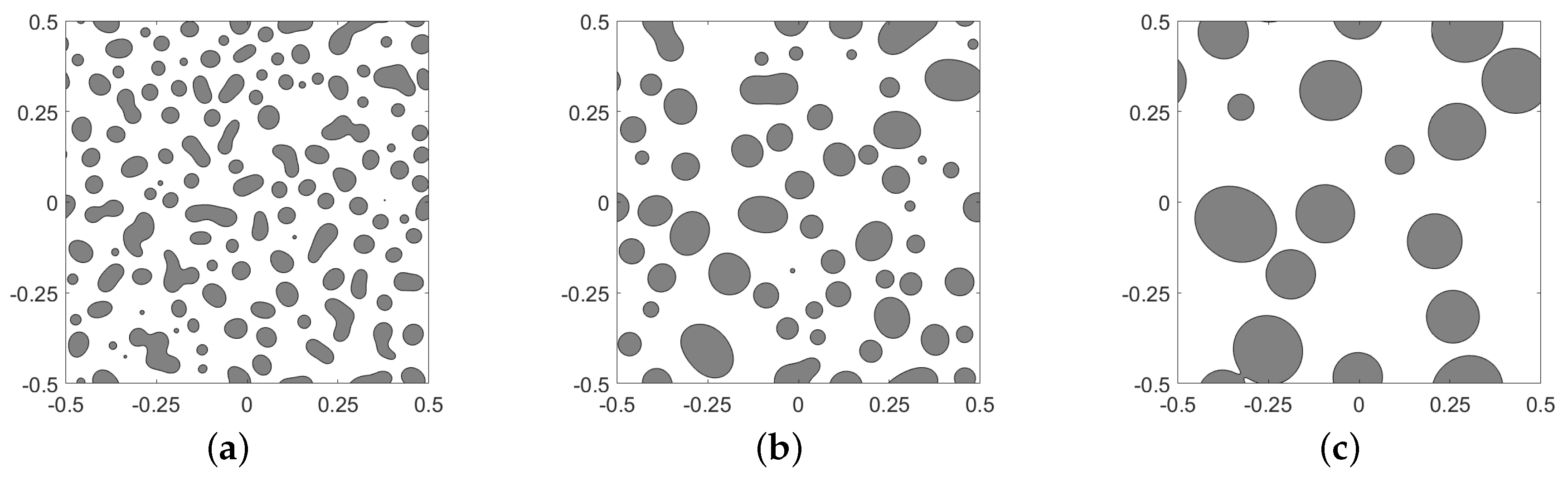
Figure 9.
(a–c) are the snapshots of numerical solutions of the Cahn–Hilliard (CH) equation with the initial condition (39) using the Fourier-spectral method at , , and , respectively.
Figure 9.
(a–c) are the snapshots of numerical solutions of the Cahn–Hilliard (CH) equation with the initial condition (39) using the Fourier-spectral method at , , and , respectively.

Figure 10.
(a–c) are the snapshots of numerical solutions of the CH equation with the initial condition (40) at , , and , respectively.
Figure 10.
(a–c) are the snapshots of numerical solutions of the CH equation with the initial condition (40) at , , and , respectively.

Figure 11.
Energy dissipation over time to the CH equation with the initial condition (39).
Figure 11.
Energy dissipation over time to the CH equation with the initial condition (39).

Figure 12.
(a–c) are the snapshots of numerical solutions of the nonlocal CH model (4) with the initial condition (43) at , , and , respectively. For colored figures, see the manuscript of web version.

Figure 13.
(a–c) are the snapshots of numerical solutions of the nonlocal CH model (4) with the initial condition (44) at , , and , respectively. For colored figures, see the manuscript of web version.

Figure 14.
Energy dissipation over time to the nonlocal CH model (4) with the initial condition (43). Note that t-axis is on log-scale.

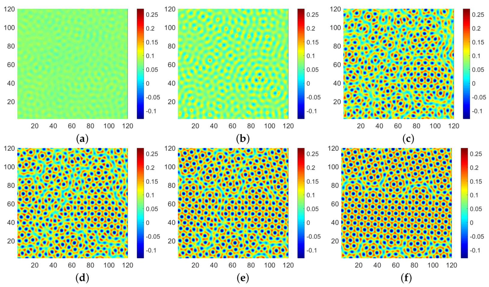
Figure 15.
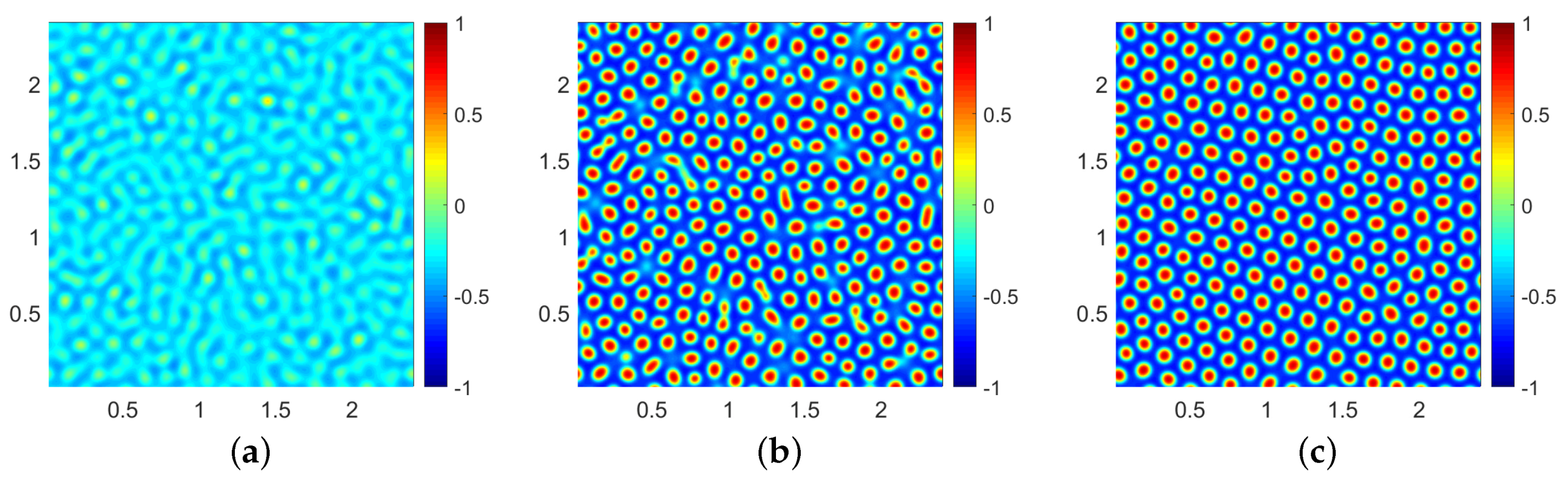
(a–f) are the snapshots of numerical solutions of the SH equation with the initial condition (47) at , , , 30,000, 60,000, and 150,000, respectively. For colored figures, see the manuscript of web version.
Figure 15.
(a–f) are the snapshots of numerical solutions of the SH equation with the initial condition (47) at , , , 30,000, 60,000, and 150,000, respectively. For colored figures, see the manuscript of web version.

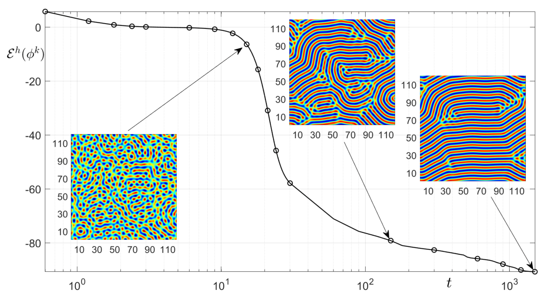
Figure 16.
Energy dissipation over time of Equation (49) to the SH equation with the initial condition (47). Note that t-axis is on log-scale.

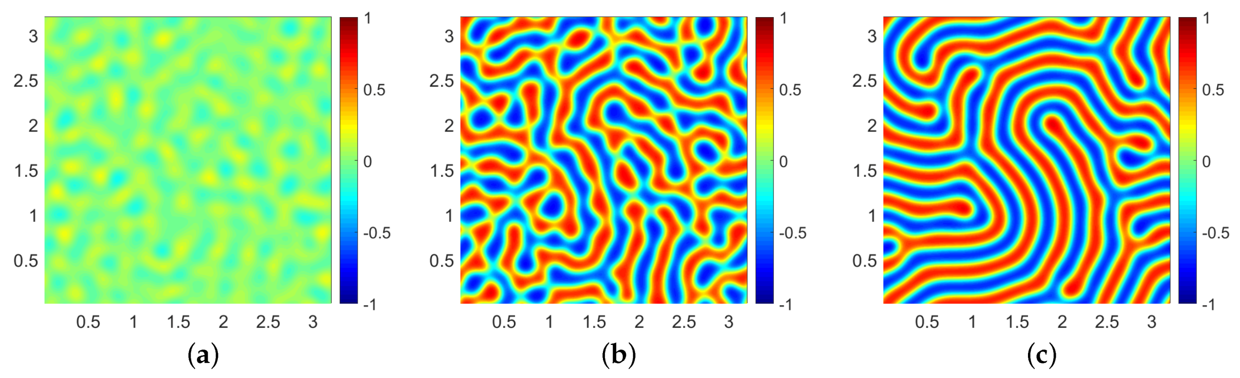
Figure 17.
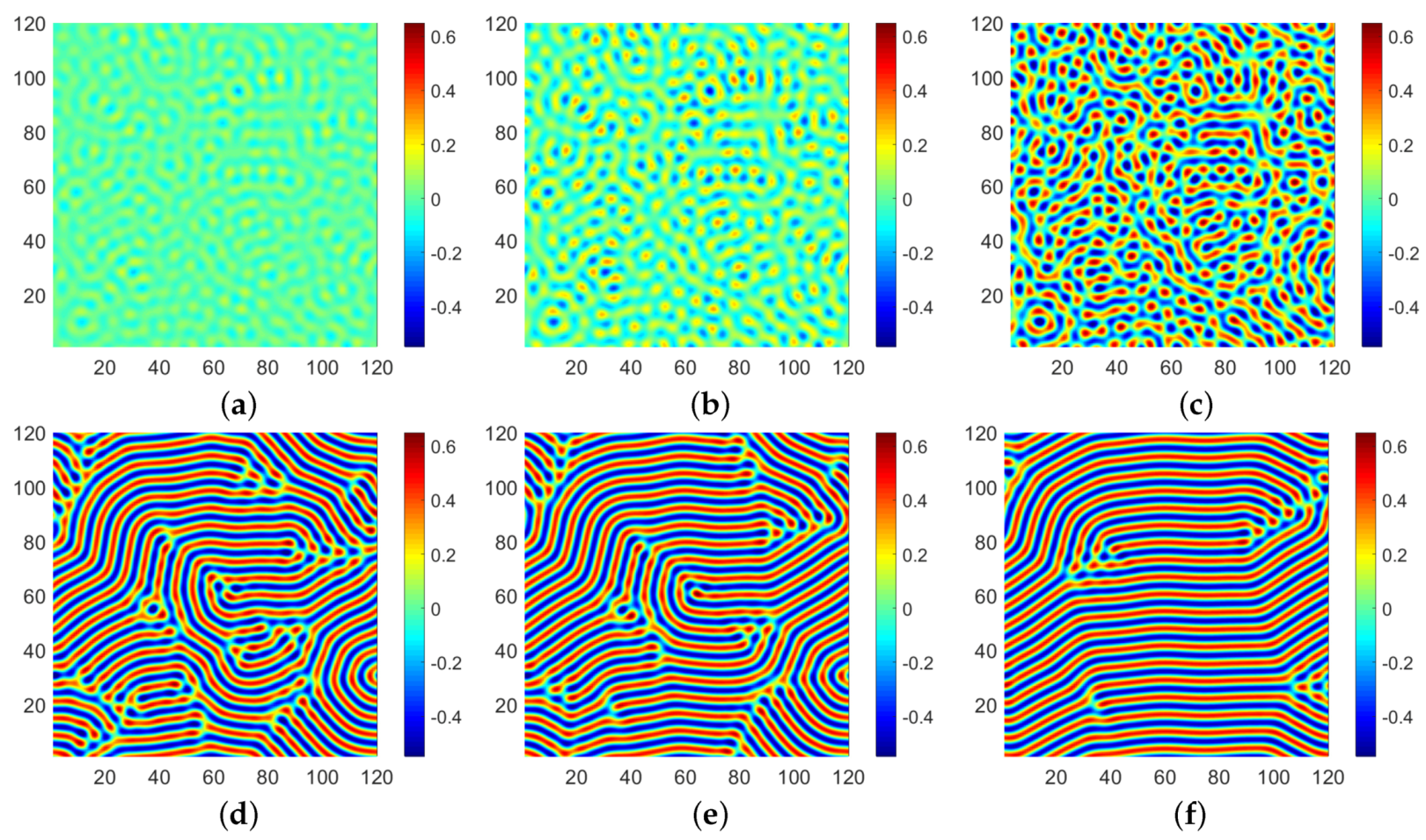
(a–f) are the snapshots of numerical solutions of the classical phase-field crystal (PFC) model with the initial condition (50) at 30,000, 210,000, 450,000, 600,000, 900,000, and 1,500,000, respectively. For colored figures, see the manuscript of web version.
Figure 17.
(a–f) are the snapshots of numerical solutions of the classical phase-field crystal (PFC) model with the initial condition (50) at 30,000, 210,000, 450,000, 600,000, 900,000, and 1,500,000, respectively. For colored figures, see the manuscript of web version.

Figure 18.
Energy dissipation over time, Equation (49), to the classical PFC model with the initial condition (50). Note that t-axis is on log-scale.

Figure 19.
(a–d) are the snapshots of numerical solutions of the molecular beam epitaxy (MBE) growth model employing the initial condition (51) at , , , and 15,000, respectively. For colored figures, see the manuscript of web version.
Figure 19.
(a–d) are the snapshots of numerical solutions of the molecular beam epitaxy (MBE) growth model employing the initial condition (51) at , , , and 15,000, respectively. For colored figures, see the manuscript of web version.

Figure 20.
Energy decay over time to the MBE model. Note that t-axis is on log-scale.

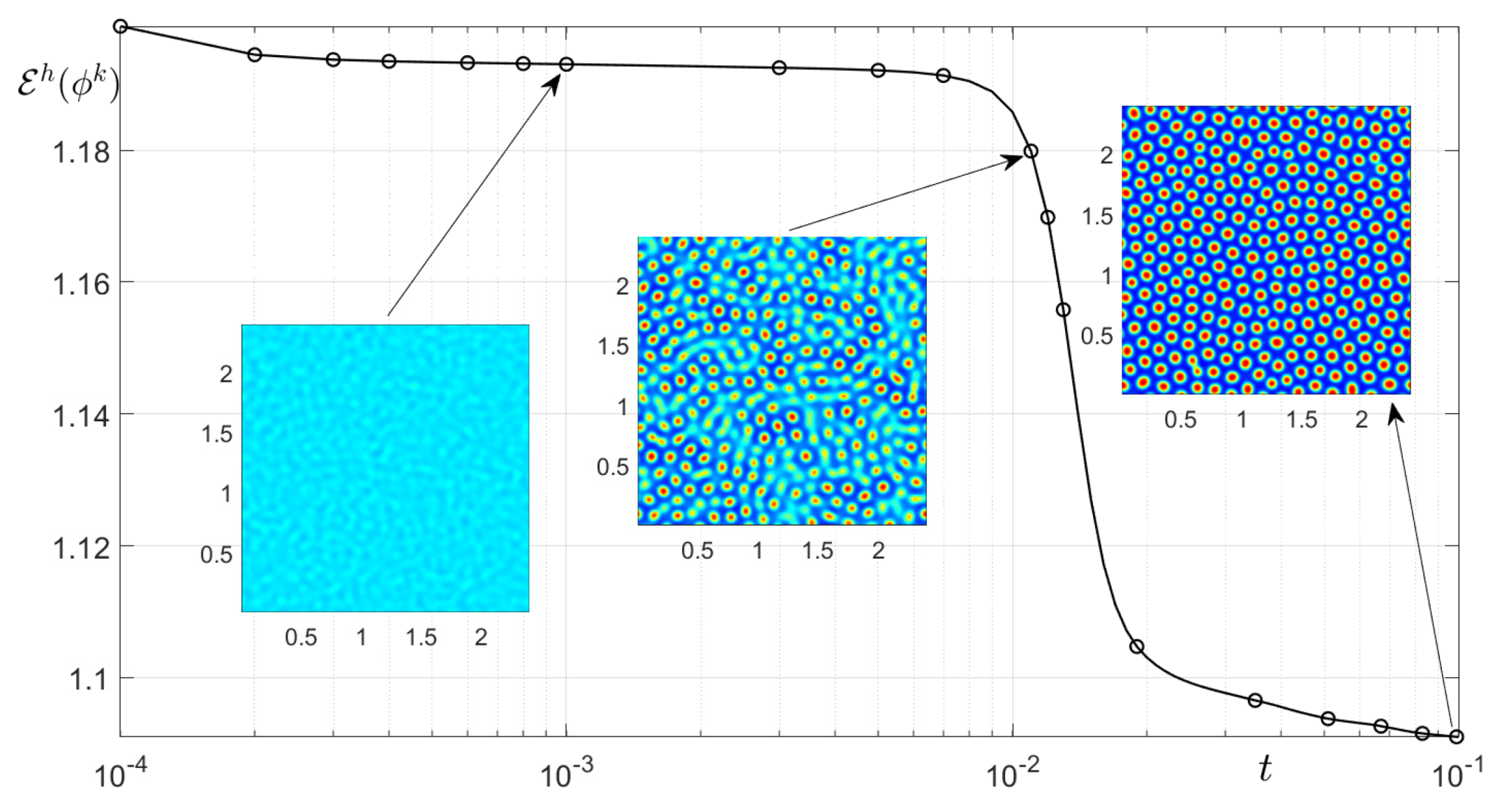
Figure 21.
Logarithmic Flory–Huggins free energy with and .

Figure 22.
(a–c) are the zero-level contours over time with the AC Equation (2) with the logarithmic Flory–Huggins free energy (55) and the initial condition (60) at , , and , respectively.

Figure 23.
(a–c) are the snapshots of numerical solutions of the CH equation with the logarithmic Flory–Huggins free energy (55) and the initial condition (40) at , , and , respectively.
Figure 23.
(a–c) are the snapshots of numerical solutions of the CH equation with the logarithmic Flory–Huggins free energy (55) and the initial condition (40) at , , and , respectively.

Figure 24.
(a) Initial condition (77). (b,c) are the snapshots of zero level set to the numerical solutions of the AC equation using the Fourier-spectral method after 480 and 800 iterations with , respectively.
Figure 24.
(a) Initial condition (77). (b,c) are the snapshots of zero level set to the numerical solutions of the AC equation using the Fourier-spectral method after 480 and 800 iterations with , respectively.

Figure 25.
Temporal evolutions of the AC equation using the Fourier-spectral method with (a) Equation (78) and (b) Equation (79). From left to right, the evolutionary times at each column are , and , respectively.
Figure 25.
Temporal evolutions of the AC equation using the Fourier-spectral method with (a) Equation (78) and (b) Equation (79). From left to right, the evolutionary times at each column are , and , respectively.

Figure 26.
Energy dissipation over time to the AC equation with the initial condition (77).
Figure 26.
Energy dissipation over time to the AC equation with the initial condition (77).

Figure 27.
With the initial condition (81), (a–c) are the snapshots of zero level set to the numerical solutions of the CH equation using the Fourier-spectral method after and 1000 iterations with , respectively.
Figure 27.
With the initial condition (81), (a–c) are the snapshots of zero level set to the numerical solutions of the CH equation using the Fourier-spectral method after and 1000 iterations with , respectively.

Figure 28.
Temporal evolutions of the CH equation with the initial condition (82) using the Fourier-spectral method. (a–c) are the snapshots of zero level set to the numerical solutions at , , and with , respectively.
Figure 28.
Temporal evolutions of the CH equation with the initial condition (82) using the Fourier-spectral method. (a–c) are the snapshots of zero level set to the numerical solutions at , , and with , respectively.

Figure 29.
Energy dissipation over time to the CH equation with the initial condition (81).
Figure 29.
Energy dissipation over time to the CH equation with the initial condition (81).

Figure 30.
(a–c) are the snapshots of the spherical pattern formation via nonlocal CH equation at , , and 10,000, respectively.
Figure 30.
(a–c) are the snapshots of the spherical pattern formation via nonlocal CH equation at , , and 10,000, respectively.

Figure 31.
(a–c) are the snapshots of the lamellar pattern formation via nonlocal CH equation at , , and 10,000, respectively.
Figure 31.
(a–c) are the snapshots of the lamellar pattern formation via nonlocal CH equation at , , and 10,000, respectively.

Figure 32.
Energy dissipation over time of Equation (85) via nonlocal CH equation with the initial condition (84). Each snapshot depicts the evolution at , , and 10,000, respectively. Note that t-axis is on log-scale.

Figure 33.
Temporal evolutions of the SH equation with the initial condition (86) using the Fourier-spectral method. (a–f) are snapshots at , , , 14,000, 20,000, and 24,000, respectively.
Figure 33.
Temporal evolutions of the SH equation with the initial condition (86) using the Fourier-spectral method. (a–f) are snapshots at , , , 14,000, 20,000, and 24,000, respectively.

Figure 34.
Energy dissipation over time of Equation (87) via SH equation with the initial condition (86). Each snapshot depicts the evolution at , , and 24,000, respectively. Note that t-axis is on log-scale.

Figure 35.
Temporal evolutions of the SH equation with the initial condition (88) using the Fourier-spectral method. (a–f) are snapshots at , 300, 450, 600, 900, and 1500, respectively.
Figure 35.
Temporal evolutions of the SH equation with the initial condition (88) using the Fourier-spectral method. (a–f) are snapshots at , 300, 450, 600, 900, and 1500, respectively.


© 2020 by the authors. Licensee MDPI, Basel, Switzerland. This article is an open access article distributed under the terms and conditions of the Creative Commons Attribution (CC BY) license (http://creativecommons.org/licenses/by/4.0/).
Share and Cite
MDPI and ACS Style
Yoon, S.; Jeong, D.; Lee, C.; Kim, H.; Kim, S.; Lee, H.G.; Kim, J. Fourier-Spectral Method for the Phase-Field Equations. Mathematics 2020, 8, 1385. https://0-doi-org.brum.beds.ac.uk/10.3390/math8081385
AMA Style
Yoon S, Jeong D, Lee C, Kim H, Kim S, Lee HG, Kim J. Fourier-Spectral Method for the Phase-Field Equations. Mathematics. 2020; 8(8):1385. https://0-doi-org.brum.beds.ac.uk/10.3390/math8081385
Chicago/Turabian StyleYoon, Sungha, Darae Jeong, Chaeyoung Lee, Hyundong Kim, Sangkwon Kim, Hyun Geun Lee, and Junseok Kim. 2020. "Fourier-Spectral Method for the Phase-Field Equations" Mathematics 8, no. 8: 1385. https://0-doi-org.brum.beds.ac.uk/10.3390/math8081385
Note that from the first issue of 2016, this journal uses article numbers instead of page numbers. See further details here.