On the Characteristic Polynomial of the Generalized k-Distance Tribonacci Sequences


Department of Mathematics, Faculty of Science, University of Hradec Králové, 500 03 Hradec Králové, Czech Republic
Mathematics 2020, 8(8), 1387; https://0-doi-org.brum.beds.ac.uk/10.3390/math8081387
Submission received: 6 August 2020
/
Revised: 17 August 2020
/
Accepted: 18 August 2020
/
Published: 18 August 2020
(This article belongs to the Special Issue New Insights in Algebra, Discrete Mathematics, and Number Theory)
Abstract
:In 2008, I. Włoch introduced a new generalization of Pell numbers. She used special initial conditions so that this sequence describes the total number of special families of subsets of the set of n integers. In this paper, we prove some results about the roots of the characteristic polynomial of this sequence, but we will consider general initial conditions. Since there are currently several types of generalizations of the Pell sequence, it is very difficult for anyone to realize what type of sequence an author really means. Thus, we will call this sequence the generalized k-distance Tribonacci sequence .
Keywords:
Fibonacci numbers; Tribonacci numbers; generalized Fibonacci numbers; characteristic equation; Descartes’ sign rule; Eneström–Kakeya theoremMSC:
11A63; 11B39; 11J861. Introduction
The Fibonacci numbers was first described in connection with computing the number of descendants of a pair of rabbits in the book Liber Abaci in 1202 (see [1], pp. 404–405). This sequence is probably one of the best known recurrent sequences and it is defined by the second order recurrence (firstly used by Albert Girard in 1634, see [2], p. 393)
with initial values and . The Fibonacci numbers have the a closed form expression for the computation (without appealing to its recurrence) of the nth Fibonacci number. It is called Binet’s formula in honor of Jacques Binet, which discovered this formula in 1843 (see [2] or [3], p. 394),
where and are the roots of the characteristic equation . The Fibonacci numbers have been the main object of many books and papers (see for example [4,5,6,7,8,9] and some references therein). Many generalizations of the Fibonacci sequence have appeared in the literature. Probably the most well-known generalization are the k-generalized Fibonacci sequence (also known as the k-bonacci, the k-fold Fibonacci or k-th order Fibonacci), satisfying
with initial values (for ) and . For instance, for , we have the usual Fibonacci numbers and for , we get the Tribonacci numbers (see Feinberg’s introductory paper [10] and Spickerman’s paper [11] with properties of roots of its characteristic equation). Miles [12] seems to be the introductory paper of this generalization. In 1971, Miller [13] proved some basic facts on the geometry of the roots of their characteristic equation , what was the bases for gradually finding the “Binet-like” formula for the sequence (see [14,15,16]) and for some properties of this sequence, see, for instance [17,18,19,20,21,22,23,24,25,26,27,28,29].
In 2008, Włoch [30] studied the total number of k-independent sets in some special simple, undirected graphs. She showed that this number is equal to the terms of the sequence , where these numbers are defined for an integer by
with initial values
She called these numbers the generalized Pell numbers, but we think that this notation is quite unclear as there are already many types of generalized Pell sequences and as this sequence is defined by “four terms recurrence relation” as the Tribonacci sequence, so we will call this sequence generalized k-distance Tribonacci sequence (the notation “k-distance’’ is very suitable as it was introduced in the same meaning, e.g., in papers [31,32,33]).
In this work, we are interested in the sequence defined by the recurrence Equation (2), but with general initial values , for an integer (where are real numbers, previously chosen). Let be characteristic polynomial of this sequence. Note that has roots which are the generators of the Pell sequence (by its “Binet-like” formula)
In fact, coincide with the Pell sequence (for the choice of and ), while, the sequence coincides with the Tribonacci sequence .
As the properties of roots of turned out important for its deeper study, in this paper, we shall study the behavior (in the algebraic and analytic sense) of the roots of . More precisely, our main result is the following:
Theorem 1.
For , let be the characteristic polynomial of . Then the following hold
- (i)
- has a dominant root, say , which is its only positive root, withfor all . In particular, tends to as .
- (ii)
- has a negative root (which is unique) only when k is even.
- (iii)
- All the roots of are simple roots.
- (iv)
- is a strictly decreasing sequence.
2. Auxiliary Results
In this section, we shall present two results which will be essential ingredients in the proof of our results. For clarity, we record some notations. As usual, denotes the set , for integers . Also, denotes the closed unit ball (i.e., all complex numbers z such that ) and is defined as the set of all complex zeros of the polynomial .
The first tool is the famous Descartes’ sign rule which gives an upper bound on the number of positive or negative real roots of a polynomial with real coefficients. For the sake of completeness, we shall state it as a lemma.
Lemma 1
(Descartes’ sign rule). Let be a polynomial with nonzero real coefficients and such that . Set
Then, there exists a non-negative integer r such that (multiple roots of the same value are counted separately).
As a corollary, we have that for obtaining information on the number of negative real roots, we must apply the previous rule for .
Remark 1.
Generally speaking, the previous result says that if the terms of a single-variable polynomial with real coefficients are ordered by descending variable exponent, then the number of positive roots of the polynomial is equal to the number of sign differences between consecutive nonzero coefficients, minus an even non-negative integer.
A fundamental result in the theory of recurrence sequences asserts that:
Lemma 2.
Let be a linear recurrence sequence whose characteristic polynomial splits as
where the ’s are distinct complex numbers. Then, there exist uniquely determined non-zero polynomials , with ( is the multiplicity of as zero of ), for , such that
The proof of this result can be found in [34], Theorem C.1.
Another useful and very important result is due to Eneström and Kakeya [35,36]:
Lemma 3
(Eneström-Kakeya theorem). Let be an n-degree polynomial with real coefficients. If , then all zeros of lie in .
Now, we are ready to deal with the proof of the theorem.
3. The Proof of the Main Theorem
3.1. Proof of Item (i)
Proof.
By Lemma 1, the polynomial has only a positive root, say . From now on, by abuse of notation, we shall write f for and for . By using that , we obtain that , where
We claim that if z is a root of , then . In fact, it suffices to prove that all the roots of belong to . This holds by applying Lemma 3 to the polynomial
since (this last inequality is valid because ).
Now, since is the only positive root of and , then , for all (also, ). Our second claim is that if z is root of with , then z is a real number. Indeed, since . then . On the other hand, the triangle inequality yields and so
Thus implying that and lie in the same ray. In particular, there are real numbers and such that and . Thus and are real numbers and by subtracting them, we deduce that so is . Therefore, is also a real number, as desired.
In conclusion, if z is a root of with , then z is a real number with . Thus, . However, leads to the absurdity as or (according to k is even or odd, respectively). Therefore, is the dominant root of .
To finish the proof of this item, we must prove that
For that, it is enough to show that and . In fact, and, since , we have
where we used the Bernoulli’s inequality: for every integer an every real number (note that ). □
3.2. Proof of Item (ii)
Proof.
By using Lemma 1 and the fact that (for k even), then has exactly one negative root.
For the case in which k is odd, we have that and so, again by Lemma 1, we infer that the number of negative roots of is either 0 or 2. Thus, we need to find another approach to conclude that there is no such that , when k is odd. To prove this, it suffices to show that , for and , for all . In fact, , since while , for (here we used that is even and so ). Furthermore, is positive, for , since (because is odd), while for . This finishes the proof. □
3.3. Proof of Item (iii)
Proof.
Aiming for a contradiction, suppose that z is a double root of . Then, . Since , then and . Thus,
and so
Hence, we obtain
yielding that . Therefore, , where
Since are both real numbers, then if , we infer that . However, implying that which leads to the absurd that . In the case in which , we use that the negative root of f satisfies (since k is even and then and ) and after some manipulations, we arrive again at the absurdity of . In conclusion, such a root z does not exist and so, all the roots of are simple roots. □
3.4. Proof of Item (iv)
Proof.
We now wish to prove that . For ease of notation, set and . Let us define the polynomial . Since (for and ), then is an increasing function. Note that and the relation , implies that . Since, by item (i), , and , then . In conclusion, yielding that the sequence is strictly decreasing. □
4. Applications of Our Results
In this section, we shall show an application of our results for the distribution of the dominant root depending on k and the determination of its upper bound (of course this is also an upper bound to the absolute value of all the other roots). For example, by Theorem 1 and Lemma 2, we can write a k-distance Tribonacci sequence in its asymptotic form
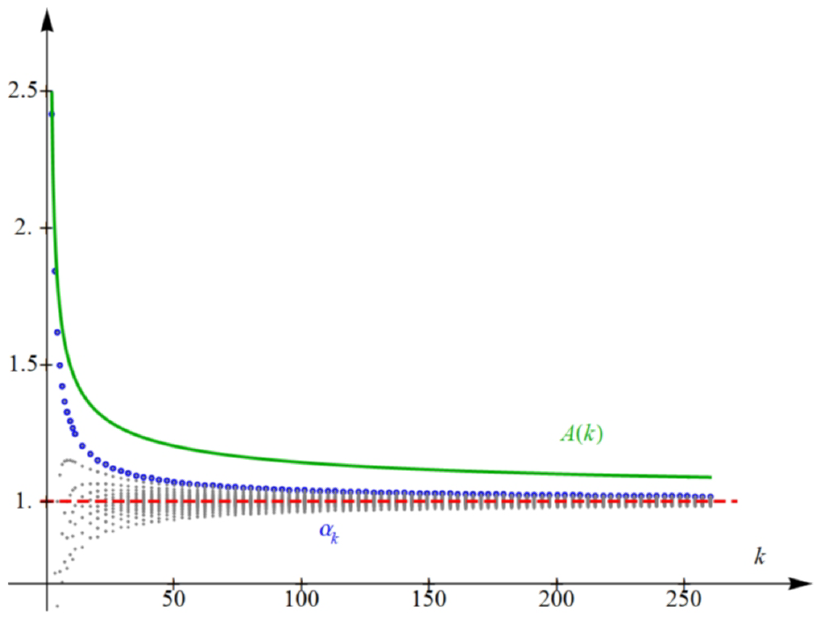
where c is a nonzero constant and is a function which tends to 0 as . Therefore, the growth of is a crucial step to gain an understanding about the growth of the sequence . This behavior and its precision is showed in the Table 1, Figure 1 and Figure 2.
5. Conclusions
In this paper, we have been interested in the behavior of the so-called k-distance Tribonacci sequence which is a kth order recurrence defined by . There exist many results in literature which permit transfer the study of the behavior of the sequence to the knowledge of the analytic and algebraic properties of roots of its characteristic polynomial (in a form of a “Binet-like formula”). In our case, this polynomial is . Therefore, in this work, we shall explicit a complete study of the roots of . For example, in our main result, we shall prove (among other things) the existence of a dominant root (together with some more accurate lower and upper bounds), for all . Moreover, we shall show that is a strictly decreasing sequence (which converges to 1 as ).
Funding
The author was supported by Project of Excelence PrF UHK No. 2215/2020, University of Hradec Králové, Czech Republic.
Acknowledgments
The author is very grateful for the support of the University of Hradec Králové.
Conflicts of Interest
The author declares no conflict of interest.
References
- Sigler, L.E. Fibonacci’s Liber Abaci: A translation into Modern English of Leonardo Pisano’s Book of Calculation; Springer: New York, NY, USA, 2002. [Google Scholar]
- Dickson, L.E. History Theory of Numbers: Divisibility and Primality; AMS Chelsea Publishing: New York, NY, USA, 1952. [Google Scholar]
- Binet, M.J. Mémoire sur l’intégration des équations linéaires aux différences finies, d’un ordre quelconque, à coefficients variables. Comptes Rendus des Séances de l’Académie des Sciences 1843, 17, 559–567. [Google Scholar]
- Kalman, D.; Mena, R. The Fibonacci Numbers–Exposed. Math. Mag. 2003, 76, 167–181. [Google Scholar]
- Koshy, T. Fibonacci and Lucas Numbers with Applications; Wiley: New York, NY, USA, 2001. [Google Scholar]
- Posamentier, A.S.; Lehmann, I. The (Fabulous) Fibonacci Numbers; Prometheus Books: Amherst, NY, USA, 2007. [Google Scholar]
- Vorobiev, N.N. Fibonacci Numbers; Birkhäuser: Basel, Switzerland, 2003. [Google Scholar]
- Hoggat, V.E. Fibonacci and Lucas Numbers; Houghton-Mifflin: PaloAlto, CA, USA, 1969. [Google Scholar]
- Ribenboim, P. My Numbers, My Friends: Popular Lectures on Number Theory; Springer: New York, NY, USA, 2000. [Google Scholar]
- Feinberg, M. Fibonacci-Tribonacci. Fibonacci Q. 1963, 1, 70–74. [Google Scholar]
- Spickerman, W.R. Binet’s Formula for the Tribonacci Sequence. Fibonacci Q. 1982, 20, 118–120. [Google Scholar]
- Miles, E.P., Jr. Generalized Fibonacci Numbers and Associated Matrices. Am. Math. Mon. 1960, 67, 745–752. [Google Scholar] [CrossRef]
- Miller, M.D. On generalized Fibonacci numbers. Am. Math. Mon. 1971, 78, 1108–1109. [Google Scholar] [CrossRef]
- Spickerman, W.R.; Joyner, R.N. Binet’s Formula for the Recursive Sequence of Order k. Fibonacci Q. 1984, 22, 327–331. [Google Scholar]
- Wolfram, D.A. Solving generalized Fibonacci recurrences. Fibonacci Q. 1998, 36, 129–145. [Google Scholar]
- Dresden, G.P.B.; Du, Z. A Simplified Binet Formula for k-Generalized Fibonacci Numbers. J. Integer Seq. 2014, 17, 1–9. [Google Scholar]
- Marques, D. On k-generalized Fibonacci numbers with only one distinct digit. Util. Math. 2015, 98, 23–31. [Google Scholar]
- Bravo, J.J.; Luca, F. On a conjecture about repdigits in k-generalized Fibonacci sequences. Publ. Math. Debr. 2013, 82, 3–4. [Google Scholar] [CrossRef]
- Noe, T.D.; Post, J.V. Primes in Fibonacci n-step and Lucas n-step sequences. J. Integer Seq. 2005, 8, 05.4.4. [Google Scholar]
- Marques, D. The proof of a conjecture concerning the intersection of k-generalized Fibonacci sequences. Bull. Braz. Math. Soc. 2013, 44, 455–468. [Google Scholar] [CrossRef] [Green Version]
- Bravo, J.J.; Luca, F. Coincidences in generalized Fibonacci sequences. J. Number Theory 2013, 133, 2121–2137. [Google Scholar] [CrossRef]
- Chaves, A.P.; Marques, D. A Diophantine equation related to the sum of squares of consecutive k-generalized Fibonacci numbers. Fibonacci Q. 2014, 52, 70–74. [Google Scholar]
- Gómez Ruiz, C.A.; Luca, F. Multiplicative independence in k-generalized Fibonacci sequences. Lith. Math. J. 2016, 56, 503–517. [Google Scholar] [CrossRef]
- Bednařík, D.; Freitas, G.; Marques, D.; Trojovský, P. On the sum of squares of consecutive k-bonacci numbers which are l-bonacci numbers. Colloq. Math. 2019, 156, 153–164. [Google Scholar] [CrossRef]
- Trojovský, P. On Terms of Generalized Fibonacci Sequences which are Powers of their Indexes. Mathematics 2019, 7, 700. [Google Scholar] [CrossRef] [Green Version]
- Siar, Z.; Erduvan, F.; Keskin, R. Repdigits as product of two Pell or Pell-Lucas numbers. Acta Math. Univ. Comenian. 2019, 88, 247–256. [Google Scholar]
- Ddamulira, M.; Luca, F. On the x-coordinates of Pell equations which are k-generalized Fibonacci numbers. J. Number Theory 2020, 207, 156–195. [Google Scholar] [CrossRef]
- Ddamulira, M. Repdigits as sums of three Padovan number. Boletín de la Sociedad Matemática Mexicana 2020, 26, 1–15. [Google Scholar] [CrossRef] [PubMed] [Green Version]
- Chaves, A.P.; Trojovský, P. A Quadratic Diophantine Equation Involving Generalized Fibonacci Numbers. Mathematics 2020, 8, 1010. [Google Scholar] [CrossRef]
- Włoch, I. On generalized Pell numbers and their graph representations. Comment. Math. 2008, 48, 169–175. [Google Scholar]
- Włoch, I.; Bednarz, U.; Bród, D.; Wołowiec-Musiał, M.; Włoch, A. On a new type of distance Fibonacci numbers. Discrete Appl. Math. 2013, 161, 2695–2701. [Google Scholar] [CrossRef]
- Bród, D.; Piejko, K.; Włoch, I. Distance Fibonacci numbers, distance Lucas numbers and their applications. Ars Comb. 2013, 112, 397–409. [Google Scholar]
- Piejko, K.; Włoch, I. On k-Distance Pell Numbers in 3-Edge-Coloured Graphs. J. Appl. Math. 2014, 2014, 428020. [Google Scholar] [CrossRef] [Green Version]
- Shorey, T.N.; Tijdeman, R. Exponential Diophantine Equations; Cambridge Tracts in Mathematics 87; Cambridge University Press: Cambridge, UK, 1986. [Google Scholar]
- Eneström, G. Remarque sur un théorème relatif aux racines de l’equation anxn+an−1xn−1+⋯+a1x+a0=0 où tous les coefficientes a sont réels et positifs. Tohoku Math. J. (1) 1920, 18, 34–36. [Google Scholar]
- Kakeya, S. On the limits of the roots of an algebraic equation with positive coefficients. Tohoku Math. J. (1) 1912, 2, 140–142. [Google Scholar]
Figure 1.
The graph of dominant roots (colored by blue) of , its upper bound (colored by green) and absolute value of the other roots of (colored by gray) for .
Figure 1.
The graph of dominant roots (colored by blue) of , its upper bound (colored by green) and absolute value of the other roots of (colored by gray) for .

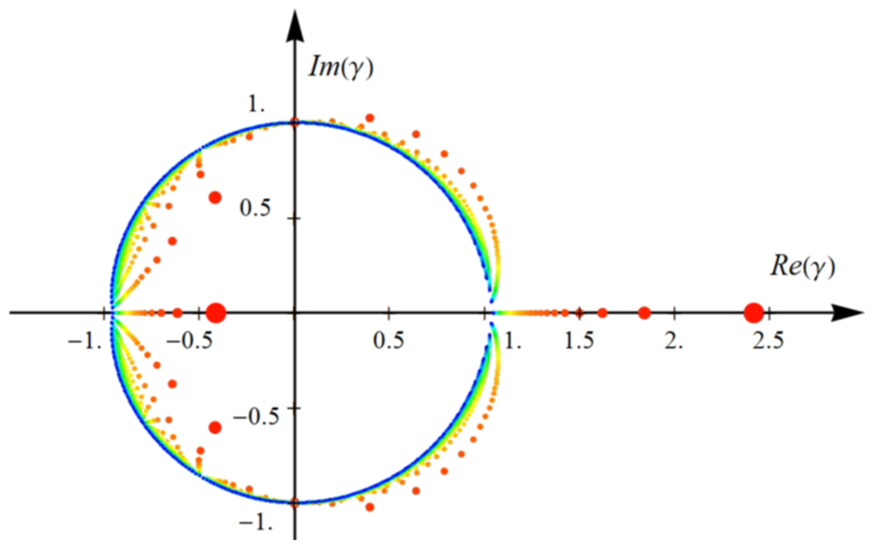
Figure 2.
The graph of all roots of for . We performed coloring points that correspond to the roots , in a manner that with increasing values of k decreased the size of the points, and their color changed gradually from warm colors to cold colors.
Figure 2.
The graph of all roots of for . We performed coloring points that correspond to the roots , in a manner that with increasing values of k decreased the size of the points, and their color changed gradually from warm colors to cold colors.


Table 1.
The dominant root of and its upper bound for k from 2 to 49.
| k | k | k | ||||||
|---|---|---|---|---|---|---|---|---|
| 2 | 2.414213562 | 2.414213562 | 18 | 1.163910449 | 1.342997170 | 34 | 1.097462321 | 1.246182982 |
| 3 | 1.839286755 | 2.000000000 | 19 | 1.156780140 | 1.333333333 | 35 | 1.095189446 | 1.242535625 |
| 4 | 1.618033989 | 1.816496581 | 20 | 1.150313062 | 1.324442842 | 36 | 1.093031609 | 1.239045722 |
| 5 | 1.497094049 | 1.707106781 | 21 | 1.144417473 | 1.316227766 | 37 | 1.090979976 | 1.235702260 |
| 6 | 1.419632763 | 1.632455532 | 22 | 1.139018098 | 1.308606700 | 38 | 1.089026607 | 1.232495277 |
| 7 | 1.365254707 | 1.577350269 | 23 | 1.134052557 | 1.301511345 | 39 | 1.087164353 | 1.229415734 |
| 8 | 1.324717957 | 1.534522484 | 24 | 1.129468689 | 1.294883912 | 40 | 1.085386751 | 1.226455407 |
| 9 | 1.293188036 | 1.500000000 | 25 | 1.125222520 | 1.288675135 | 41 | 1.083687949 | 1.223606798 |
| 10 | 1.267874775 | 1.471404521 | 26 | 1.121276701 | 1.282842712 | 42 | 1.082062631 | 1.220863052 |
| 11 | 1.247047862 | 1.447213595 | 27 | 1.117599293 | 1.277350098 | 43 | 1.080505957 | 1.218217890 |
| 12 | 1.229573607 | 1.426401433 | 28 | 1.114162811 | 1.272165527 | 44 | 1.079013511 | 1.215665546 |
| 13 | 1.214676212 | 1.408248290 | 29 | 1.110943467 | 1.267261242 | 45 | 1.077581254 | 1.213200716 |
| 14 | 1.201805729 | 1.392232270 | 30 | 1.107920561 | 1.262612866 | 46 | 1.076205487 | 1.210818511 |
| 15 | 1.190560750 | 1.377964473 | 31 | 1.105075990 | 1.258198890 | 47 | 1.074882811 | 1.208514414 |
| 16 | 1.180640991 | 1.365148372 | 32 | 1.102393848 | 1.254000254 | 48 | 1.073610101 | 1.206284249 |
| 17 | 1.171817047 | 1.353553391 | 33 | 1.099860103 | 1.250000000 | 49 | 1.072384476 | 1.204124145 |
© 2020 by the author. Licensee MDPI, Basel, Switzerland. This article is an open access article distributed under the terms and conditions of the Creative Commons Attribution (CC BY) license (http://creativecommons.org/licenses/by/4.0/).
Share and Cite
MDPI and ACS Style
Trojovský, P. On the Characteristic Polynomial of the Generalized k-Distance Tribonacci Sequences. Mathematics 2020, 8, 1387. https://0-doi-org.brum.beds.ac.uk/10.3390/math8081387
AMA Style
Trojovský P. On the Characteristic Polynomial of the Generalized k-Distance Tribonacci Sequences. Mathematics. 2020; 8(8):1387. https://0-doi-org.brum.beds.ac.uk/10.3390/math8081387
Chicago/Turabian StyleTrojovský, Pavel. 2020. "On the Characteristic Polynomial of the Generalized k-Distance Tribonacci Sequences" Mathematics 8, no. 8: 1387. https://0-doi-org.brum.beds.ac.uk/10.3390/math8081387
Note that from the first issue of 2016, this journal uses article numbers instead of page numbers. See further details here.