On Fundamental Solution for Autonomous Linear Retarded Functional Differential Equations

Abstract

This document focuses attention on the fundamental solution of an autonomous linear retarded functional differential equation (RFDE) along with its supporting cast of actors: kernel matrix, characteristic matrix, resolvent matrix; and the Laplace transform. The fundamental solution is presented in the form of the convolutional powers of the kernel matrix in the manner of a convolutional exponential matrix function. The fundamental solution combined with a solution representation gives an exact expression in explicit form for the solution of an RFDE. Algebraic graph theory is applied to the RFDE in the form of a weighted loop-digraph to illuminate the system structure and system dynamics and to identify the strong and weak components. Examples are provided in the document to elucidate the behavior of the fundamental solution. The paper introduces fundamental solutions of other functional differential equations.

1. Introduction

This paper examines and characterizes the fundamental matrix solution for the n-vector autonomous linear retarded functional differential equation (RFDE)

$$\begin{array}{cc}\hfill x^{\prime }(t)& =\underset{0}{\overset{a}{\int }}A(ds)x(t-s)+f(t),t>0,\hfill \end{array}$$

(1)

with forcing function $f(t)$ and initial function $h(\theta )$

$$\begin{array}{cc}\hfill x(\theta )& =h(\theta ),-a\le \theta \le 0,\hfill \end{array}$$

(2)

where $x(t)$ is an n-vector, the kernel matrix $A(ds)$ is an $n\times n$ matrix of Borel measures with support on the interval $[0,a]$, and f and g belong to function spaces that will be described in Section 2.

We shall consider the case that

$$A(ds)=\sum _{i=0}^N{A}_i\delta (s-{\theta }_i)+A(s)ds,$$

(3)

where $0={\theta }_0<{\theta }_1\cdots <{\theta }_N=a$, $A_i$ are $n\times n$ matrices over $\mathbb{R}$, $\delta (s)$ is the Dirac delta function, and $A(s)$ is an integrable $n\times n$ matrix function on the interval $[0,a]$. Consequently, in terms of the Radon–Nikodym theorem, $A(ds)$ has an absolutely continuous part $A(s)$, a discrete singular part with a finite number of point masses (atoms) corresponding to Dirac delta measures, and a zero continuous singular part. It will be evident from the context whether the symbol A refers to an $n\times n$ matrix over Borel measures, an $n\times n$ matrix over the real numbers, or a matrix function. The terms ${\sum }_{i=0}^N{A}_i\delta (s-{\theta }_i)$ and $A(s)ds$ respectively correspond to discrete delays and distributed delay of the kernel matrix $A(ds)$.

The fundamental solution $\Phi (t)$ satisfies the RFDE

$$\begin{array}{cc}\hfill {\Phi }^{\prime }(t)& =\underset{0}{\overset{a}{\int }}A(ds)\Phi (t-s),t>0,\hfill \end{array}$$

(4)

with initial conditions

$$\begin{array}{cc}\hfill \Phi (0)& =I,\Phi (t)=O\mathrm{for}t<0,\hfill \end{array}$$

(5)

where I and O are respectively the $n\times n$ identity and zero matrices. Note that the fundamental solution $\Phi (t)$ also satisfies the Volterra integro-differential equation

$$\begin{array}{cc}\hfill {\Phi }^{\prime }(t)& =\underset{0}{\overset{t}{\int }}A(ds)\Phi (t-s),t>0,\hfill \end{array}$$

(6)

with initial condition

$$\begin{array}{cc}\hfill \Phi (0)& =I.\hfill \end{array}$$

(7)

Theorem 1.

The fundamental solution $\Phi (t)$ is given by

$$\Phi (t)=\sum _{n=0}^{\infty }\frac{1}{n!}\underset{0}{\overset{t}{\int }}{A}^n(ds){(t-s)}^n,$$

(8)

where the convolutional powers of the kernel matrix $A^n(ds)$ are defined by

1. 

$A^0(ds)=I\delta (s)$,

2. 

$A^1(ds)=A(ds)$, and

3. 

$A^n(ds)=A^{n-1}(ds)\ast A^1(ds)$ for $n\ge 2$,

where ∗ denotes the convolution of two matrix measures.

Proof. 

See the proof of Theorem 2. □

This expression for the fundamental solution in the case $n=1$ can be found in References [1,2,3]. Note that the computation for the fundamental solution $\Phi (t)$ is simplified by the restriction of a finite number of discrete atoms in the discrete singular component, and a zero continuous singular component.

The fundamental solution $\Phi (t)$ for the autonomous linear ordinary differential equation (ODE) ${\Phi }^{\prime }(t)=A\Phi (t)$ is given (see Reference [4]) by the exponential matrix function

$$\Phi (t)=\sum _{n=0}^{\infty }\frac{1}{n!}{(At)}^n=exp(At).$$

(9)

Note that the fundamental solution $\Phi (t)$ in Equation (8) for the RFDE is analogous to and is a generalization of the fundamental solution in Equation (9) for the ODE, and that it has the form of a convolutional exponential matrix function.

Equation (4) establishes a relationship between two actors in an RFDE: the fundamental solution $\Phi (t)$ and the kernel matrix $A(ds)$. Let us consider the other actors and their roles.

For $z\in \mathbb{C}$ the Laplace transform $\mathcal{L}$ (see Reference [5]) of the fundamental solution $\Phi (t)$ is

$$\mathcal{L}(\Phi (t))(z)=\widehat{\Phi }(z)=\underset{0}{\overset{\infty }{\int }}{e}^{-zt}\Phi (t)dt.$$

(10)

Definition 1.

We define the characteristic matrix $\Delta (z)=zI-\underset{0}{\overset{a}{\int }}A(ds)e^{-zs}$, the characteristic determinant $det(\Delta (z))$, and the resolvent matrix ${\Delta }^{-1}(z)$.

We shall show in Section 4.1 that $\widehat{\Phi }(z)={\Delta }^{-1}(z)$ or alternatively $\Phi (t)={\mathcal{L}}^{-1}({\Delta }^{-1}(z))$, so that the fundamental solution $\Phi (t)$ is the inverse Laplace of the resolvent matrix ${\Delta }^{-1}(z)$.

The fundamental solution $\Phi (t)$ can also be expressed in the form of Laplace inverse as a contour integral in the z-plane

$${\Phi }_{ci}(t)=\frac{1}{2\pi i}{\int }_{(c)}{e}^{zt}{\Delta }^{-1}(z)dz,$$

(11)

where contributions to the integral arise from the characteristic roots $\{{\lambda }_j\}$ with multiplicity $m_r$ of the characteristic determinant $D(z)=det(\Delta (z))=0$. We shall show in Section 4 that this gives rise to a spectral representation of the fundamental solution $\Phi (t)$ in terms of the exponential solutions of the RFDE

$${\Phi }_{ci}(t)=\sum _r\sum _{j=0}^{m_r-1}{\Psi }_{rj}{t}^{j}exp({\lambda }_{r}t).$$

(12)

In the case that all characteristic roots ${\lambda }_r$ are simple with multiplicity $m_r=1$, we have

$${\Phi }_{ci}(t)=\sum _r{\Psi }_{r}exp({\lambda }_{r}t),$$

(13)

where ${\Psi }_r=C({\lambda }_r)/D^{\prime }({\lambda }_r)$ with $C(z)=\mathrm{adj}(\Delta (z))$. The characteristic roots $\{{\lambda }_r\}$ can be arranged in some appropriate order, such as decreasing real part $\Re ({\lambda }_r)$ or increasing modulus $|{\lambda }_r|$.

It is known (References [6,7,8,9]) that ${\Phi }_{ci}(t)$ is convergent for a range of values of t, where $-a\le t<na$. The case $t=-a$ arises in the scalar case in which the exponential solutions are complete and independent (see Reference [10]). Even where convergence is not an issue, we could have ${\Phi }_{ci}(t)\ne \Phi (t)$ for $t<t_0$ and ${\Phi }_{ci}(t)\equiv \Phi (t)$ for $t\ge t_0$, as shown in the example in Section 4.4, where $t_0=2a$. An open question is to characterize the minimum time $t_0$ for the equality of ${\Phi }_{ci}(t)$ and $\Phi (t)$ given by $t_0={inf}_{\tau >-a}\{\tau ;{\Phi }_{ci}(t)\equiv \Phi (t)\mathrm{for}t>\tau \}$. Note that ${\Phi }_{ci}(t)$ plays the role of a spectral representation of the fundamental solution $\Phi (t)$ for $t>t_0$.

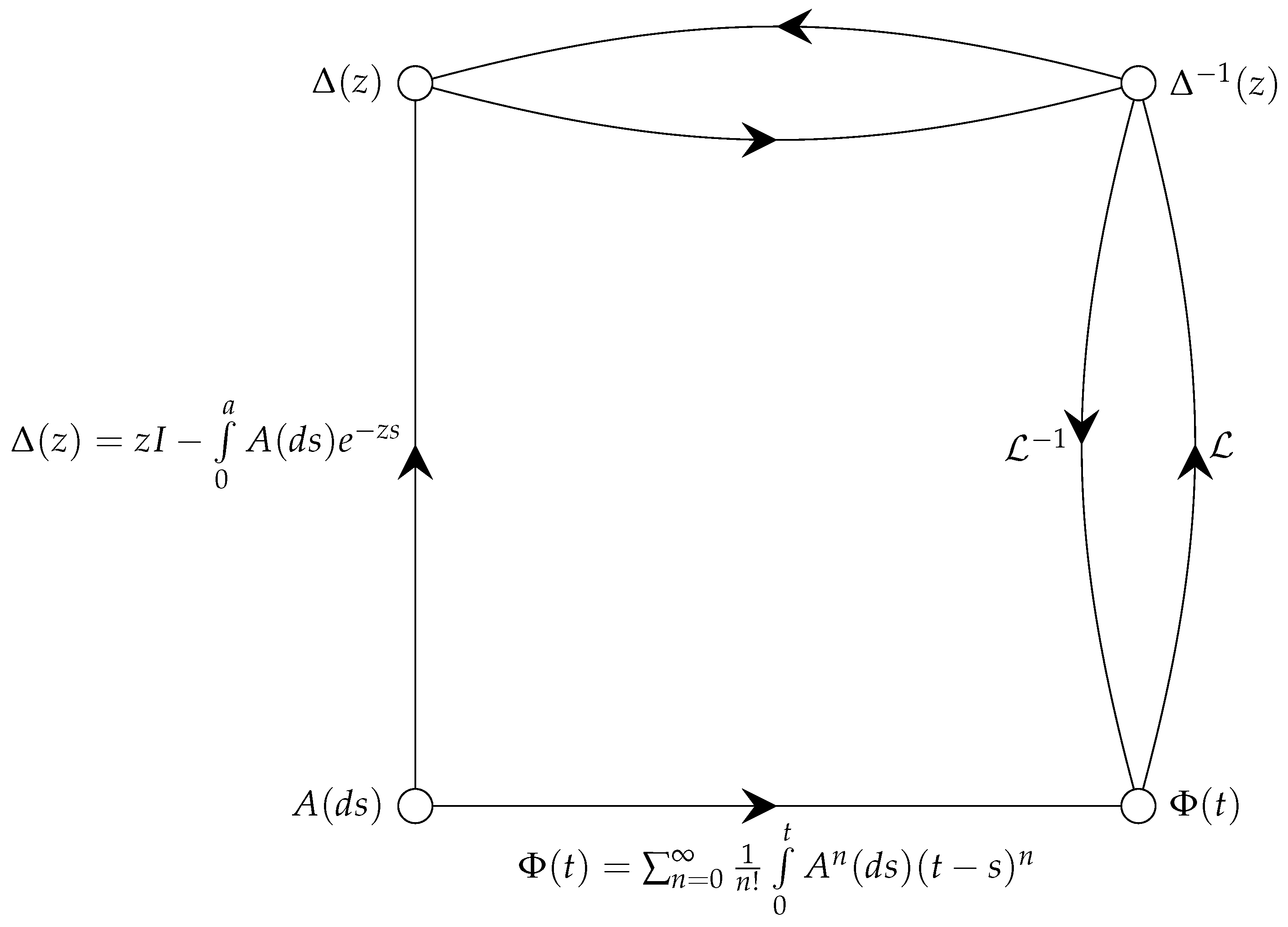
Figure 1 shows the relationship between the RFDE actors: the kernel matrix $A(ds)$, the fundamental solution $\Phi (t)$, the characteristic matrix $\Delta (z)$, and the resolvent matrix ${\Delta }^{-1}(z)$. Note that Figure 1 shows two different routes to determine the fundamental solution $\Phi (t)$ from the kernel matrix $A(ds)$: (i) the direct route from Equation (8), and (ii) the indirect route through the characteristic matrix, the resolvent matrix, and the Laplace inverse. Depending on circumstances, either route may be preferable.

On its own, the fundamental solution is a representative proxy for the solutions of the RFDE. For example, the fundamental solution has exponential bounds that determine the asymptotic behavior of the RFDE solutions. Also the fundamental solution combined with a solution representation gives an exact expression in explicit form for the solution of an RFDE. However, the explicit form of the fundamental solution does not in and of itself convey all the information on its properties. It is the diversity of actors and their interplay that brings a variety of perspectives and the full force to bear on extracting information on the RFDE.

Remark 1.

The right hand side of the linear autonomous RFDE (1) is expressed as

$$\underset{0}{\overset{a}{\int }}A(ds)x(t-s)insteadof\underset{-a}{\overset{0}{\int }}{A}^{\prime }(ds)x(t+s)$$

(14)

where $A^{\prime }(ds)=A(-ds)$, to emphasize the convolution nature of the linear autonomous RFDE (see page 77 of Reference [11]), to highlight the convolutional composition of the fundamental solution, and to reflect the situation that for a linear autonomous RFDE essentially every operation is a convolution.

Remark 2.

The use of measures in the kernel matrix of the RFDE in Equation (1) is chosen over the alternatives of (i) distributions and (ii) functions of normalized bounded variation. This choice is mainly a matter of style. Whatever choice is made, the fundamental solution will involve convolutional powers of the kernel matrix.

Some monographs dealing with the study of functional differential equations and related Volterra integro-differential equations are References [7,11,12,13,14,15,16,17,18].

The remainder of the paper is organized as follows: Section 2 on preliminaries establishes the foundation for the paper. Section 3 applies algebraic graph theory to study RFDEs. It uses a weighted loop-digraph representation of an RFDE to illuminate the system structure, connectivity, and dynamics. The characteristics of the fundamental solution are explored in Section 4. Examples are considered in the main body of the document to elucidate the behavior of the fundamental solution to an RFDE. Section 5 extends the fundamental solution to other functional differential equations. Finally, the conclusions are presented in Section 6.

2. Preliminaries

2.1. Ring of Borel Measures

Consider the set ${\mathbb{B}}_{cs}^{+}$ of Borel measures on ${\mathbb{R}}^{+}$ with compact support of the form

$$a(ds)=\sum _{i=0}^N{a}_i\delta (s-{\theta }_i)+a(s)ds$$

(15)

with finite number of atoms at $\{{\theta }_i\}$, $0={\theta }_0<{\theta }_1\cdots <{\theta }_N$, $a_i\in \mathbb{R}$, and integrable function $a(s)$.

The addition operator + is given by

$$(a+b)(ds)=a(ds)+b(ds)=\sum _{i=0}^N{a}_i\delta (s-{\theta }_i)+\sum _{i=0}^M{b}_i\delta (s-{\eta }_i)+a(s)ds+b(s)ds,$$

(16)

and convolution (aka multiplication) operator ∗ is given by

$$\begin{array}{}\hfill \mathrm{(17)}& \begin{array}{cc}\hfill (a\ast b)(ds)=a(ds)\ast b(ds)& ={\displaystyle \sum _{i=0}^N}{\displaystyle \sum _{j=0}^M}{a}_i{b}_j\delta (s-{\theta }_i-{\eta }_j)+{\displaystyle \sum _{i=0}^N}{a}_{i}b(s-{\theta }_i)ds\hfill \end{array}\hfill \hfill \mathrm{(18)}& \begin{array}{cc}\hfill & +{\displaystyle \sum _{j=0}^M}{b}_{j}a(s-{\eta }_j)ds+(a\ast b)(s)ds,\hfill \end{array}\hfill \end{array}$$

where

$$b(ds)=\sum _{j=0}^M{b}_j\delta (s-{\eta }_j)+b(s)ds.$$

(19)

It is straightforward to show that ${\mathbb{B}}_{cs}^{+}={\mathbb{B}}_{cs}^{+}(+,\ast )$ is a commutative ring, with additive identity $0(ds)$ such that $(0+a)(ds)=a(ds)$, and the multiplicative identity the Dirac delta measure $\delta (ds)$ such that $\delta (s)\ast a(ds)=a(ds)$.

Definition 2.

For $a(ds)\in {\mathbb{B}}_{cs}^{+}$ define norm $\left|a(ds)\right|={sup}_{|f(x)|\le 1}\int a(ds)f(s)$.

Define the support $\mathrm{supp}(a(ds))$ as the complement in ${\mathbb{R}}^{+}$ of the set $X=\{x:\underset{N_x}{\int }a(ds)=0\}$ for all neighborhoods $N_x$ of x that are sufficiently small.

We have the following standard results:

• $|(a\ast b)(ds)|\le |a(ds)||b(ds)|$.
• $\mathrm{supp}((a+b)(ds)))\subseteq \mathrm{supp}(a(ds))\bigcup \mathrm{supp}(b(ds))$.
• $\mathrm{supp}((a\ast b)(ds)))\subseteq \mathrm{supp}(a(ds))+\mathrm{supp}(b(ds))$.

In particular, if $\mathrm{supp}(a(ds))\subseteq [0,d]$, $\mathrm{supp}(a^n(ds))\subseteq [0,nd]$.

2.2. Matrix over Ring of Borel Measures

Definition 3.

A $n\times n$ matrix over a ring of Borel measures $M_n({\mathbb{B}}_{cs}^{+})$ is a $n\times n$ array of elements of the ring ${\mathbb{B}}_{cs}^{+}$.

We have matrix addition

$$C(ds)=(A+B)(ds)=A(ds)+B(ds)with{c}_{ij}(ds)=a_{ij}(ds)+b_{ij}(ds)$$

(20)

and matrix convolution (multiplication)

$$C(ds)=(A\ast B)(ds)=A(ds)\ast B(ds)with{c}_{ij}(ds)=\sum _{k=0}^n{a}_{ik}(ds)\ast b_{kj}(ds).$$

(21)

Note that the kernel matrix $A(ds)\in M_n({\mathbb{B}}_{cs}^{+})$, and well as its its convolutional powers $A^n(ds)\in M_n({\mathbb{B}}_{cs}^{+})$.

Definition 4.

A matrix norm $\left|\right|A\left|\right|$ for $A\in M_n(\mathbb{R})$ with addition and multiplication defined conventionally on the ring $\mathbb{R}$ has the following properties:

1. 

$\left|\right|A\left|\right|\ge 0Nonnegative$

2. 

$\left|\right|A\left|\right|=0\iff A=0Positive$

3. 

$\left|\right|cA\left|\right|=\left|c\right|\left|\right|A\left|\right|,c\in \mathbb{R}Homogeneous$

4. 

$\left|\right|A+B\left|\right|\le \left|\right|A\left|\right|+\left|\right|B\left|\right|TriangleInequality$

5. 

$\left|\right|AB\left|\right|\le \left|\right|A\left|\right|\left|\right|B\left|\right|Submultiplicativity$

Particular instances of matrix norms are the $l_1$-norm ${\left|\right|A\left|\right|}_1={\sum }_{i=j=1}^n\left|a_{ij}\right|$ and the Frobenius $l_2$-norm ${\left|\right|A\left|\right|}_2=({\sum }_{i=j=1}^n|a_{ij}{{|}^2)}^{\frac{1}{2}}$. See Section 5.6 of Reference [19].

2.3. Fundamental Solution

We now turn our attention to the Volterra integro-differential equation of convolutional type satisfied by the fundamental solution for an RFDE

$${\Phi }^{\prime }(t)=\underset{0}{\overset{t}{\int }}A(ds)\Phi (t-s),t>0,\Phi (0)=I.$$

(22)

By integrating we obtain the equivalent Volterra integral equation of convolutional type

$$\Phi (t)=I+\underset{0}{\overset{t}{\int }}dsB(s)\Phi (t-s),t\ge 0,$$

(23)

where the kernel matrix function

$$B(t)=\underset{0}{\overset{t}{\int }}A(ds)=\sum _{i=0}^N{A}_{i}H(t-{\theta }_i)+\underset{0}{\overset{min(t,a)}{\int }}d\theta A(\theta ),$$

(24)

with

$$H(t)=\left\{\begin{array}{cc}1,\hfill & t\ge 0,\hfill \\ 0,\hfill & t<0.\hfill \end{array}\right.$$

(25)

It is well known that this Volterra integral equation has a Liouville–Neumann series solution in the form

$$\Phi (t)=I+\sum _{n=1}^{\infty }\underset{0}{\overset{t}{\int }}{B}^n(s)ds$$

(26)

where matrix functions $B^n(t)$ are defined by $B^1=B$, and $B^n=B^{n-1}\ast B^1$ where ∗ denotes a convolution of two matrix functions. This form of the fundamental solution is promulgated in References [14,15,20].

Proposition 1.

The two forms of the fundamental solution

$$\Phi (t)=\sum _{n=0}^{\infty }\frac{1}{n!}\underset{0}{\overset{t}{\int }}{A}^n(ds){(t-s)}^n\mathrm{and}\Phi (t)=I+\sum _{n=1}^{\infty }\underset{0}{\overset{t}{\int }}{B}^n(s)ds$$

(27)

are equivalent.

Proof. 

Since $B(t)=\underset{0}{\overset{t}{\int }}A(ds)$, we have $\mathcal{L}((B(t))(z)=\widehat{B}(z)=\widehat{A}(z)/z$.

$$\mathcal{L}\left(\underset{0}{\overset{t}{\int }}{B}^n(s)ds\right)={(\widehat{B}(z))}^n/z={(\widehat{A}(z))}^n/z^{n+1}.$$

(28)

$$\mathcal{L}\left(\frac{1}{n!}\underset{0}{\overset{t}{\int }}{A}^n(ds){(t-s)}^n\right)=\frac{1}{n!}\mathcal{L}(A^n(ds))\mathcal{L}(t^n)={(\widehat{A}(z))}^n/z^{n+1}.$$

(29)

Hence from equality of Laplace transforms $\frac{1}{n!}\underset{0}{\overset{t}{\int }}{A}^n(ds){(t-s)}^n=\underset{0}{\overset{t}{\int }}{B}^n(s)ds$ for $n\ge 1$. □

Theorem 2.

The solution of ${\Phi }^{\prime }(t)=\underset{0}{\overset{t}{\int }}A(ds)\Phi (t-s)$ with $\Phi (0)=I$ exists in a form

$$\Phi (t)=\sum _{n=0}^{\infty }\frac{1}{n!}\underset{0}{\overset{t}{\int }}{A}^n(ds){(t-s)}^n.$$

(30)

The solution $\Phi (t)$ is unique and has continuous dependence on the kernel matrix $A(ds)$.

Proof. 

For $t\in [0,T]$ where $T<\infty$ we have

$$\left|\right|\sum _{n=0}^{\infty }\frac{1}{n!}\underset{0}{\overset{t}{\int }}{A}^n(ds){(t-s)}^n\left|\right|\le \sum _{n=0}^{\infty }\frac{1}{n!}{K}^n{T}^n=exp(KT)$$

(31)

so that the series converges absolutely and uniformly, thereby justifying the formal procedures in the following steps:

$$\begin{array}{}\hfill \mathrm{(32)}& \begin{array}{cc}\hfill {\Phi }^{\prime }(t)& ={\displaystyle \sum _{n=1}^{\infty }}\frac{1}{(n-1)!}\underset{0}{\overset{t}{\int }}{A}^n(ds){(t-s)}^{n-1}={\displaystyle \sum _{n=0}^{\infty }}\frac{1}{n!}\underset{0}{\overset{t}{\int }}{A}^{n+1}(ds){(t-s)}^n\hfill \end{array}\hfill \hfill \mathrm{(33)}& \begin{array}{cc}\hfill & ={\displaystyle \sum _{n=0}^{\infty }}\frac{1}{n!}\underset{0}{\overset{t}{\int }}A(du)\underset{0}{\overset{t-u}{\int }}{(t-s-u)}^n={\int }_0^{t}A(du){\displaystyle \sum _{n=0}^{\infty }}\frac{1}{n!}\underset{0}{\overset{t-u}{\int }}{A}^n(ds){(t-s-u)}^n\hfill \end{array}\hfill \hfill \mathrm{(34)}& \begin{array}{cc}\hfill & =\underset{0}{\overset{t}{\int }}A(du)\Phi (t-u).\hfill \end{array}\hfill \end{array}$$

Intermediate steps are

$$\begin{array}{}\hfill \mathrm{(35)}& \begin{array}{cc}\hfill \underset{0}{\overset{t}{\int }}{A}^{n+1}(ds){(t-s)}^n& =\underset{0}{\overset{t}{\int }}\underset{0}{\overset{s}{\int }}A(du)A^n(d(s-u)){(t-s)}^n=\underset{0}{\overset{t}{\int }}A(du)\underset{u}{\overset{t}{\int }}{A}^n(d(s-u)){(t-s)}^n\hfill \end{array}\hfill \hfill \mathrm{(36)}& \begin{array}{cc}\hfill & =\underset{0}{\overset{t}{\int }}A(du)\underset{0}{\overset{t-u}{\int }}{A}^n(ds){(t-s-u)}^n.\hfill \end{array}\hfill \end{array}$$

Hence $\Phi (t)$ is a solution.

To show that the solution is unique, suppose that we have two solutions ${\Phi }_1(t)$ and ${\Phi }_2(t)$ so that for the Volterra integral equation we have

$${\Phi }_1(t)-{\Phi }_2(t)=\underset{0}{\overset{t}{\int }}B(t-s)[{\Phi }_1(s)-{\Phi }_2(s)]ds.$$

(37)

Consequently

$$\left|\right|{\Phi }_1(t)-{\Phi }_2(t)\left|\right|<ϵ+\underset{0}{\overset{t}{\int }}K\left|\right|{\Phi }_1(s)-{\Phi }_2(s)\left|\right|ds$$

(38)

for some constant $K>0$, arbitrarily small $ϵ>0$, and $0\le t\le T$. From Gronwall’s inequality (see page 24 of Reference [21]) we have $\left|\right|{\Phi }_1(t)-{\Phi }_2(t)\left|\right|\le ϵexp(Kt)$. However, since $ϵ$ is arbitrarily small, we have $\left|\right|{\Phi }_1(t)-{\Phi }_2(t)\left|\right|=0$ and consequently ${\Phi }_1(t)={\Phi }_2(t)$.

To demonstrate continuous dependence on the kernel matrix $A(ds)$, consider two solutions ${\Phi }_1(t)$ and ${\Phi }_2(t)$ of

$${\Phi }_1(t)=I+\underset{0}{\overset{t}{\int }}{B}_1(t-s){\Phi }_1(s)ds\mathrm{and}{\Phi }_2(t)=I+\underset{0}{\overset{t}{\int }}{B}_2(t-s){\Phi }_2(s)ds.$$

(39)

We can write

$${\Phi }_1(t)-{\Phi }_2(t)=\underset{0}{\overset{t}{\int }}{B}_1(t-s)[{\Phi }_1(s)-{\Phi }_2(s)]ds+\underset{0}{\overset{t}{\int }}[B_1(t-s)-B_2(t-s)]{\Phi }_2(s)ds,$$

(40)

so that

$$\left|\right|{\Phi }_1(t)-{\Phi }_2(t)\left|\right|\le \underset{0}{\overset{t}{\int }}\left|\right|B_1(t-s)\left|\right|\left|\right|{\Phi }_1(s)-{\Phi }_2(s)\left|\right|ds+\underset{0}{\overset{t}{\int }}\left|\right|B_1(t-s)-B_2(t-s)\left|\right|\left|\right|{\Phi }_2(s)\left|\right|ds.$$

(41)

Choose $K_1>0$ so that $\left|\right|B_1(s)\left|\right|<K_1$, $K_2>0$ so that $\left|\right|{\Phi }_2(t)\left|\right|<K_2$ and $\delta =\left|\right|A_1(ds)-A_2(ds)\left|\right|$ so that $\left|\right|B_1(s)-B_2(s)\left|\right|\le T\delta$. Then

$$\left|\right|{\Phi }_1(t)-{\Phi }_2(t)\left|\right|\le \underset{0}{\overset{t}{\int }}{K}_1\left|\right|{\Phi }_1(s)-{\Phi }_2(s)\left|\right|]ds+K_2{T}^2\delta ,$$

(42)

so that by Gronwall’s inequality we have $\left|\right|{\Phi }_1(t)-{\Phi }_2(t)\left|\right|\le K_2{T}^2\delta exp(K_{1}T)$. □

We have already seen an exponential bound $\left|\right|\Phi (t)\left|\right|\le exp(KT)$ on the interval $[0,T]$. A more precise exponential bound is provided by the supremum of the real part of the characteristic roots of the characteristic determinant $det(\Delta (z))=0$.

Theorem 3

(Theorem 1.21 of Reference [15]). Let ${\alpha }_0=sup\{\Re (z);det(\Delta (z)=0\}$. For $\alpha >{\alpha }_0$$\exists K>0$ with $\left|\right|\Phi (t)\left|\right|\le Kexp(\alpha t)$ for $t\ge 0$.

Remark 3.

The term fundamental solution $\Phi (t)$ has several synonyms in the literature depending on context:

A. Cauchy matrix $C(t,s)$ for the nonautonomous RFDE

$$x^{\prime }(t)=\underset{s}{\overset{t}{\int }}A(t,d\tau )x(\tau )+f(t),t>s.$$

(43)

See page 51 of Reference [16]. For the autonomous equation $C(t,s)=\Phi (t-s)$.

B. Differential resolvent for the Volterra integro-differential equation

$$x^{\prime }(t)=\underset{0}{\overset{t}{\int }}A(ds)x(t-s)+f(t),t>0.$$

(44)

See page 77 of Reference [11].

C. Green’s function or impulse response function for RFDE

$$x^{\prime }(t)=\underset{0}{\overset{a}{\int }}A(ds)x(t-s)+f(t),t>0,$$

(45)

with $h=0$ and $f(t)=\delta (s)$. In some parts of the literature, for example Reference [16], a Green’s function is associated with a boundary value problem.

Proposition 2.

$$\underset{0}{\overset{t}{\int }}A(ds)\Phi (t-s)=\underset{0}{\overset{t}{\int }}\Phi (t-s)A(ds),$$

(46)

so that the kernel matrix and the fundamental solution commute convolutionally.

Proof. 

$$\begin{array}{}\hfill \mathrm{(47)}& \begin{array}{cc}\hfill \underset{0}{\overset{t}{\int }}A(ds)\Phi (t-s)& =A\ast \Phi =A\ast {\displaystyle \sum _{n=0}^{\infty }}\frac{1}{n!}{A}^{\ast n}\ast {(t)}^n\hfill \end{array}\hfill \hfill \mathrm{(48)}& \begin{array}{cc}\hfill & ={\displaystyle \sum _{n=0}^{\infty }}\frac{1}{n!}{A}^{\ast (n+1)}\ast {(t)}^n={\displaystyle \sum _{n=0}^{\infty }}\frac{1}{n!}{A}^{\ast n}\ast {(t)}^n\ast A\hfill \end{array}\hfill \hfill \mathrm{(49)}& \begin{array}{cc}\hfill & =\Phi \ast A=\underset{0}{\overset{t}{\int }}\Phi (t-s)A(ds),\hfill \end{array}\hfill \end{array}$$

where the steps involving an infinite sum are justified by uniform convergence. □

2.4. RFDE Solution

Standard choices for the initial function space are:

$F_1=M^2([-a,0],{\mathbb{R}}^n)$; h is Lebesgue measurable on $[-a,0]$, $h(0)$ is well defined, $\underset{-a}{\overset{0}{\int }}{\left|h(t)\right|}^{2}dt<\infty$, and ${\left|\right|h\left|\right|}_1={\{|h(0)|}^2+\underset{-a}{\overset{0}{\int }}{\left|h(t)\right|}^2{dt\}}^{1/2}$.

$F_2=C([-a,0],{\mathbb{R}}^n)$, ${\left|\right|h\left|\right|}_2={sup}_{-a\le t\le 0}\left|h(t)\right|$.

The standard choice for the forcing function space is $L_{loc}^1([0,\infty ),{\mathbb{R}}^n)$.

Results on the existence, uniqueness and continuous dependence on the initial data can be found in Reference [22] for function space $F_1$ and Reference [13] for function space $F_2$.

Theorem 4.

The representation of the solution $x(t)$ for the RFDE in Equation (1) is

$$x(t)=\Phi (t)h(0)+\underset{-a}{\overset{0}{\int }}d\alpha \underset{-\alpha }{\overset{a}{\int }}A(ds)\Phi (t-s-\alpha )h(\alpha )+\underset{0}{\overset{t}{\int }}\Phi (s)f(t-s)ds.$$

(50)

Proof. 

We first consider the case $h(0)\ne 0$, $h=0$ and $f\ne 0$. Taking the Laplace transform we obtain

$$\widehat{x}(z)=\widehat{\Phi }(z)h(0)+\widehat{\Phi }(z)\widehat{f}(z),$$

(51)

and taking the Laplace inverse, we have

$$x(t)=\Phi (t)h(0)+\underset{0}{\overset{t}{\int }}\Phi (s)f(t-s).$$

(52)

Now consider the case $h(0)=0$, $h\ne 0$, $f=0$.

Define

$$g(t)=\left\{\begin{array}{cc}\underset{t}{\overset{a}{\int }}A(s)h(t-s),\hfill & \mathrm{if}0\le t\le a,\hfill \\ 0,\hfill & \mathrm{if}t>a.\hfill \end{array}\right.$$

(53)

We have the equivalent equation

$$x^{\prime }(t)=\underset{0}{\overset{t}{\int }}A(ds)x(t-s)+g(t)$$

(54)

with $h(0)=0$ and $h=0$.

This equation has the solution

$$\begin{array}{}\hfill \mathrm{(55)}& \begin{array}{ccc}\hfill x(t)& =\underset{0}{\overset{t}{\int }}ds\Phi (t-s)\underset{s}{\overset{a}{\int }}A(du)h(s-u)\hfill & \hfill =\underset{0}{\overset{a}{\int }}ds\Phi (t-s)\underset{s}{\overset{a}{\int }}A(du)h(s-u)\end{array}\hfill \hfill \mathrm{(56)}& \begin{array}{ccc}\hfill & =\underset{-a}{\overset{0}{\int }}d\alpha \underset{-\alpha }{\overset{a}{\int }}\left[ds\right]\Phi (t-\alpha -s)A(ds)h(\alpha )\hfill & \hfill =\underset{-a}{\overset{0}{\int }}d\alpha \underset{-\alpha }{\overset{a}{\int }}A(ds)\Phi (t-\alpha -s)h(\alpha ).\end{array}\hfill \end{array}$$

From linearity, we can combine the two solutions to obtain the complete solution. □

Remark 4.

Note that the fundamental solution in combination with the representation of the solution gives an exact expression in explicit form for the solution of an RFDE.

Remark 5.

Note that the initial function h and forcing function f enter into the three constituents of the RFDE solution $x(t)$ as

1. 

Initial function point value $h(0)$ (with no history) in $\Phi (t)h(0)$,

2. 

Initial function h (with history and hereditary information) as an integrand in $\underset{-a}{\overset{0}{\int }}d\alpha \underset{-\alpha }{\overset{a}{\int }}A(ds)\Phi (t-s-\alpha )h(\alpha )$,

3. 

Forcing function f as a convolution with the fundamental solution $\Phi (t)$ in $\underset{0}{\overset{t}{\int }}\Phi (s)f(t-s)ds$.

Remark 6.

The integration region R for the double integral is

$$R=\{(\alpha ,s);-s\le \alpha \le 0,0\le s\le a\}=\{(\alpha ,s);-\alpha \le s\le a,-a\le \alpha \le 0\}.$$

(57)

The alternative expressions for the double integral are:

$$\begin{array}{}\hfill \mathrm{(58)}& \begin{array}{cc}\hfill \underset{-a}{\overset{0}{\int }}d\alpha \underset{-\alpha }{\overset{a}{\int }}A(ds)\Phi (t-s-\alpha )h(\alpha )& =\underset{-a}{\overset{0}{\int }}d\alpha \underset{-\alpha }{\overset{a}{\int }}\left[ds\right]\Phi (t-s-\alpha )A(ds)h(\alpha )\hfill \end{array}\hfill \hfill \mathrm{(59)}& \begin{array}{cc}\hfill & =\underset{0}{\overset{a}{\int }}\left[ds\right]\underset{-s}{\overset{0}{\int }}d\alpha \Phi (t-s-\alpha )A(ds)h(\alpha )\hfill \end{array}\hfill \hfill \mathrm{(60)}& \begin{array}{cc}\hfill & =\underset{0}{\overset{a}{\int }}\left[ds\right]\underset{-s}{\overset{0}{\int }}d\alpha A(ds)\Phi (t-s-\alpha )h(\alpha ).\hfill \end{array}\hfill \end{array}$$

The change in the order of integration in the double integral is justified by the Fubini theorem. The change in the order of the kernel matrix and the fundamental solution is justified since they commute convolutionally.

3. Application of Algebraic Graph Theory

In this section we apply algebraic graph theory to examine and to provide a pictorial rendition of the system structure and system dynamics of an RFDE. We also use the theory to characterize the system connectivity of the RFDE, and to identify its strong and weak components. The main reference for the application of algebraic graph theory to RFDEs is the excellent book [23].

3.1. Weighted Loop-Digraph Representation

We consider a weighted loop-digraph representation for the mathematical objects of the kernel matrix $A(ds)$ and its convolutional powers $A^n(ds)$. These mathematical objects are prominent aspects of the RFDE and its fundamental solution $\Phi (t)$.

In component form the fundamental solution $\Phi (t)$ is

$${\Phi }_{ij}(t)=H(t){\delta }_{ij}+\sum _{n=1}^{\infty }\frac{1}{n!}\underset{0}{\overset{t}{\int }}{a}_{ij}^n(ds){(t-s)}^n,$$

(61)

where

$${\delta }_{ij}=\left\{\begin{array}{cc}1,\hfill & \mathrm{if}i=j,\hfill \\ 0,\hfill & \mathrm{if}i\ne j.\hfill \end{array}\right.$$

(62)

The component form expression for the RFDE is

$$\begin{array}{}\hfill \mathrm{(63)}& \begin{array}{cc}\hfill x_i^{{}^{\prime }}(t)& ={\displaystyle \sum _{j=1}^n}\underset{0}{\overset{a}{\int }}{a}_{ij}(ds)x_j(t-s)\hfill \end{array}\hfill \hfill \mathrm{(64)}& \begin{array}{cc}\hfill & =\cdots +\underset{0}{\overset{a}{\int }}{a}_{ii}(ds)x_i(t-s)+\cdots +\underset{0}{\overset{a}{\int }}{a}_{ij}(ds)x_j(t-s)+\dots .\hfill \end{array}\hfill \end{array}$$

Likewise

$$x_j^{{}^{\prime }}(t)=\cdots +\underset{0}{\overset{a}{\int }}{a}_{jj}(ds)x_j(t-s)+\cdots +\underset{0}{\overset{a}{\int }}{a}_{ji}(ds)x_i(t-s)+\dots .$$

(65)

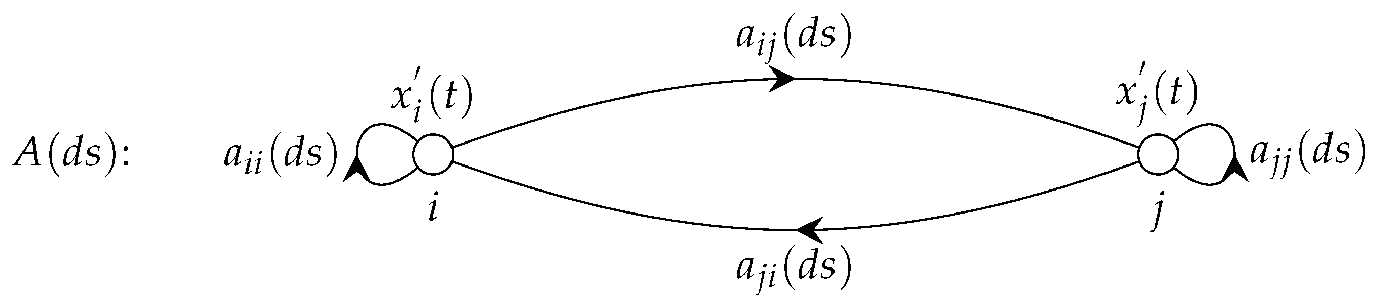
Figure 2 depicts the network structure and interactive systems dynamics for a general RFDE in the form of a weighted loop-digraph, albeit for simplicity focusing only on two nodes i and j.

Definition 5.

A weighted loop-directed graph or loop-digraph is an ordered triple $G=(V,E,W)$ where V is a set of elements called vertices (or nodes, points), and E is a set of ordered pairs of vertices called directed edges and loops. The directed edges connect two distinct vertices in the given order. Loops connect a specific vertex with itself. W is the weight assigned to each directed edge and loop.

Although for the most part the book [23] focuses on directed graphs without loops and without weights, the applied results in this paper are applicable to directed graphs with loops and weights.

Figure 2 shows a weighted loop-digraph for an n-vector RFDE. The weights assigned to directed edge $e_{ij}$ and loop $e_{ii}$ are Borel measures ${\mathbb{B}}_{cs}^{+}$ of $a_{ij}(ds)$ and $a_{ii}(ds)$, respectively. By convention the direction on the directed edge $e_{ij}$ is i to j. However, note that in a physical interpretation the influence of node j on the system dynamics at node i is represented by the Borel measure $a_{ij}(ds)$ in the opposite direction. This consideration should be borne in mind in interpreting the system dynamics from the loop-digraph.

For the components of the second convolutional power $A^2(ds)$ we have

$$a_{ij}^2(ds)=\sum _{k=1}^n(a_{ik}\ast a_{kj})(ds).$$

(66)

This has the interpretation that the Borel measure $a_{ij}^2(ds)$ is the sum of convolutions of the Borel measures encountered on the directed edges and loops on a walk of length 2 from vertex i to vertex j. More generally the Borel measure $a_{ij}^n(ds)$ is the sum of convolutions of the Borel measures encountered on the directed edges and loops on a walk of length n from vertex i to vertex j. The Borel measures $a_{ij}^n(ds)$ thus have a straightforward interpretation in the language of algebraic graph theory.

The following examples illustrate the concepts.

Example 1.

We have the RFDE

$$\begin{array}{cc}\hfill x_1^{{}^{\prime }}(t)& =x_2(t)\hfill \end{array}$$

(67)

$$\begin{array}{cc}\hfill x_2^{{}^{\prime }}(t)& =a{x}_1(t-1).\hfill \end{array}$$

(68)

The kernel matrix and its convolutional powers are

$$A(ds)=\left[\begin{array}{cc}0& \delta (s)\\ a\delta (s-1)& 0\end{array}\right],$$

(69)

$$A^{2n}(ds)=\left[\begin{array}{cc}{a}^n\delta (s-n)& 0\\ 0& a^n\delta (s-n)\end{array}\right],$$

(70)

$$A^{2n+1}(ds)=\left[\begin{array}{cc}0& a^n\delta (s-n)\\ a^{n+1}\delta (s-n-1)& 0\end{array}\right].$$

(71)

The fundamental solution is

$$\Phi (t)=\left[\begin{array}{cc}{\Phi }_{11}(t)& {\Phi }_{12}(t)\\ {\Phi }_{21}(t)& {\Phi }_{22}(t)\end{array}\right],$$

(72)

where

$$\begin{array}{cc}\hfill {\Phi }_{11}(t)& ={\Phi }_{22}=\sum _{n=0}^{\infty }\frac{1}{2n!}{a}^n{(t-n)}_{+}^{2n},\hfill \end{array}$$

(73)

$$\begin{array}{cc}\hfill {\Phi }_{12}(t)& =\sum _{n=0}^{\infty }\frac{1}{(2n+1)!}{a}^n{(t-n)}_{+}^{2n+1},\hfill \end{array}$$

(74)

$$\begin{array}{cc}\hfill {\Phi }_{21}(t)& =\sum _{n=0}^{\infty }\frac{1}{(2n+1)!}{a}^{n+1}{(t-n-1)}_{+}^{2n+1},\hfill \end{array}$$

(75)

where

$${(t)}_{+}=\left\{\begin{array}{cc}t,\hfill & ift>0,\hfill \\ 0,\hfill & ift\le 0.\hfill \end{array}\right.$$

(76)

The weighted loop-digraphs for the kernel matrix and its convolutional powers for the RFDE are shown in Figure 3.

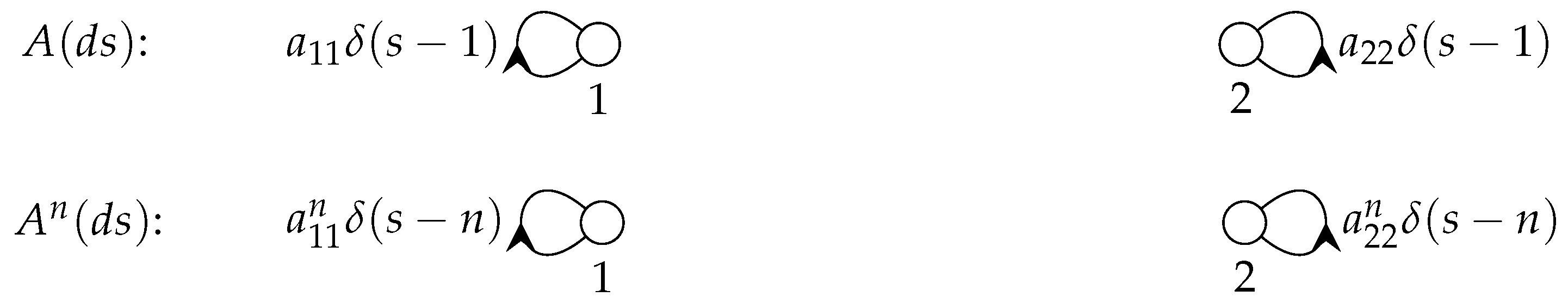
Example 2.

The RFDE is

$$x_1^{{}^{\prime }}(t)=a_{11}{x}_1(t-1)$$

(77)

$$x_2^{{}^{\prime }}(t)=a_{22}{x}_2(t-1).$$

(78)

The kernel matrix and its convolutional powers are

$$A(ds)=\left[\begin{array}{cc}{a}_{11}\delta (s-1)& 0\\ 0& a_{22}\delta (s-1)\end{array}\right],$$

(79)

$$A^n(ds)=\left[\begin{array}{cc}{a}_{11}^n\delta (s-n)& 0\\ 0& a_{22}^n\delta (s-n)\end{array}\right].$$

(80)

The fundamental solution is

$$\Phi (t)=\left[\begin{array}{cc}{\Phi }_{11}(t)& 0\\ 0& {\Phi }_{22}(t)\end{array}\right],$$

(81)

where

$$\begin{array}{cc}\hfill {\Phi }_{11}(t)& =\sum _{n=0}^{\infty }\frac{1}{n!}{a}_{11}^n{(t-n)}_{+}^n,\hfill \end{array}$$

(82)

$$\begin{array}{cc}\hfill {\Phi }_{22}(t)& =\sum _{n=0}^{\infty }\frac{1}{n!}{a}_{22}^n{(t-n)}_{+}^n.\hfill \end{array}$$

(83)

The weighted loop-digraphs for the kernel matrix and its convolutional powers for the RFDE are shown in Figure 4.

3.2. Strong and Weak Connectivity

Notice that in the first example from the previous subsection that the two components in the RFDE are interconnected and interact, and that there is no interaction in the second example. The two components are interconnected in the first example, and disconnected in the second example. The nature of the interaction between the RFDE components will be obvious in the case that the number of components is small, but less so when the number is large.

In this subsection we apply material from Chapters 2,3,5,14 of Reference [23] to characterize the connectivity between RFDE components and to classify the nature of the connectivity. Notice that this approach focuses on the structure of the RDFE, and is not concerned with the dynamics produced by the Borel measures, i.e., the weights on the directed edges and loops.

We start with some definitions.

Definition 6.

A path from $v_1$ to $v_n$ is an ordered collection of vertices $v_1,v_2\cdots v_n$ interspersed with an ordered collection of directed edges $v_1{v}_2,v_2{v}_3,\cdots ,v_{n-1}{v}_n$.

A semipath from $v_1$ to $v_n$ is an ordered collection of vertices $v_1,v_2\cdots v_n$ interspersed with an ordered collection of $n-1$ directed edges, one from each pair of directed edges $v_1{v}_2$ or $v_2{v}_1$, $v_2{v}_3$ or $v_3{v}_2$, ⋯, $v_{n-1}{v}_n$ or $v_n{v}_{n-1}$.

A strict semipath is a semipath that is not a path.

A vertex v is reachable from a vertex u if there is a path from u to v.

Points u and v are 0—connected if they are not joined by a semipath; 1—connected if they are joined by a semipath but not a path; 2—connected if they are joined by a path in one direction but not the other; 3—connected if they are joined by paths in both directions.

A loop-digraph is strongly connected or strong if every two vertices are mutually reachable.

A loop-digraph is unilaterally connected or unilateral if for any two points, at least one is reachable from the other; it is strictly unilateral if it is unilateral but not strong.

A loop-digraph is weakly connected or weak if every two vertices are joined by a semipath; it is strictly weak if it is weak but not unilateral.

A subgraph of a loop-digraph D is a loop-digraph in which the vertices and loops/directed edges are vertices and loops/directed edges of D.

A strong component of a loop-digraph is a maximal strong loop-digraph.

A unilateral component of a loop-digraph is a maximal unilateral loop-digraph.

A weak component of a loop-digraph is a maximal weak loop-digraph.

Theorem 5

(Theorem 3.2 of Reference [23]). Every vertex and every directed edge is contained in exactly one weak component.

Every vertex and every directed edge is contained in at least one unilateral component.

Every vertex and every directed edge is contained in exactly one strong component.

We shall now proceed to demonstrate how to decompose a loop-digraph into strong and weak components.

The reachability matrix $R=\left[r_{ij}\right]$ is defined as

$$r_{ij}=\left\{\begin{array}{cc}1,\hfill & \mathrm{if}\mathrm{vertex}j\mathrm{is}\mathrm{reachable}\mathrm{from}\mathrm{vertex}i,\hfill \\ 0,\hfill & \mathrm{if}\mathrm{vertex}j\mathrm{is}\mathrm{not}\mathrm{reachable}\mathrm{from}\mathrm{vertex}i.\hfill \end{array}\right.$$

(84)

In terms of the convolutional powers $A^k(ds)$ for $0\le k\le n-1$ of the kernel matrix $A(ds)$, the reachability matrix $R=\left[r_{ij}\right]$ is given by

$$r_{ij}=\left\{\begin{array}{cc}1,\hfill & \mathrm{if}{a}_{ij}^k(ds)\ne 0\mathrm{for}\mathrm{some}k,0\le k\le n-1,\hfill \\ 0,\hfill & \mathrm{otherwise}.\hfill \end{array}\right.$$

(85)

Other variants of the reachability matrix come into play:

The transpose reachability matrix $R^T=\left[r_{ij}^T\right]$ is given by

$$r_{ij}^T=\left\{\begin{array}{cc}1,\hfill & \mathrm{if}\mathrm{vertex}i\mathrm{is}\mathrm{reachable}\mathrm{from}\mathrm{vertex}j,\hfill \\ 0,\hfill & \mathrm{if}\mathrm{vertex}i\mathrm{is}\mathrm{not}\mathrm{reachable}\mathrm{from}\mathrm{vertex}j.\hfill \end{array}\right.$$

(86)

The symmetric reachability matrix $R^S=\left[r_{ij}^S\right]$ arises from the symmetrized kernel matrix $A^S(ds)$ where $a_{ij}^S(ds)=a_{ij}(ds)+a_{ji}(ds)$. It is given by

$$r_{ij}^S=\left\{\begin{array}{cc}1,\hfill & \mathrm{vertex}i\mathrm{is}\mathrm{reachable}\mathrm{from}\mathrm{vertex}j\underset{¯}{\mathrm{or}}\mathrm{vertex}j\mathrm{is}\mathrm{reachable}\mathrm{from}\mathrm{vertex}i,\hfill \\ 0,\hfill & \mathrm{otherwise}.\hfill \end{array}\right.$$

(87)

The element-wise product $R\times R^T=\left[r_{ij}^P\right]=\left[r_{ij}{r}_{ji}\right]$. It is given by

$$r_{ij}^P=\left\{\begin{array}{cc}1,\hfill & \mathrm{vertex}i\mathrm{is}\mathrm{reachable}\mathrm{from}\mathrm{vertex}j\underset{¯}{\mathrm{and}}\mathrm{vertex}j\mathrm{is}\mathrm{reachable}\mathrm{from}\mathrm{vertex}i,\hfill \\ 0,\hfill & \mathrm{otherwise}.\hfill \end{array}\right.$$

(88)

The following theorem says that the strong components of the RFDE are determined by the elementwise product reachability matrix $R\times R^T$.

Theorem 6

(Theorem 5.8 of Reference [23]). The strong component containing the vertex $v_i$ is given by the entries of 1 in the ith row (or column) in the elementwise product reachability matrix $R\times R^T$.

The following theorem says that the weak components of the RFDE are determined by the symmetric reachability matrix $R^S$.

Theorem 7

(Corollary 5.15a of Reference [23]). The weak component containing the vertex $v_i$ is given by the entries of 1 in the ith row (or column) in the symmetric reachability matrix $R^S$.

The connectedness matrix $C=\left[c_{ij}\right]$ is obtained from the reachability matrix $R=\left[r_{ij}\right]$ as follows:

If $v_i$ and $v_j$ are in the same weak component $c_{ij}=r_{ij}+r_{ji}+1$.

Otherwise $c_{ij}=0$.

The connectedness matrix $C=\left[c_{ij}\right]$ takes the values

$$c_{ij}=\left\{\begin{array}{cc}0,\hfill & \mathrm{vertices}i\mathrm{and}j\mathrm{are}\mathrm{not}\mathrm{connected}\mathrm{with}\mathrm{a}\mathrm{semipath},\mathrm{i}.\mathrm{e}.,\mathrm{they}\mathrm{are}\mathrm{disconnected},\hfill \\ 1,\hfill & \mathrm{vertices}i\mathrm{and}j\mathrm{are}\mathrm{connected}\mathrm{with}\mathrm{a}\mathrm{strict}\mathrm{semipath},\hfill \\ 2,\hfill & \mathrm{vertices}i\mathrm{and}j\mathrm{are}\mathrm{connected}\mathrm{with}\mathrm{a}\mathrm{path}\mathrm{in}\mathrm{one}\mathrm{direction}\mathrm{but}\mathrm{not}\mathrm{the}\mathrm{other},\hfill \\ 3,\hfill & \mathrm{vertices}i\mathrm{and}j\mathrm{are}\mathrm{connected}\mathrm{with}\mathrm{paths}\mathrm{in}\mathrm{both}\mathrm{directions}.\hfill \end{array}\right.$$

(89)

Definition 7.

A permutation matrix $P\in M_n({\mathbb{B}}_{cs}^{+})$ has exactly one entry in each row and in each column set to $\delta (ds)$. All other entries are 0. A permutation matrix P can be construed as relabelling the vertices in a loop-digraph.

A $n\times n$ matrix $M\in M_n({\mathbb{B}}_{cs}^{+})$ is said to be decomposable if ∃ a permutation matrix $P\in M_n({\mathbb{B}}_{cs}^{+})$ such that

$$P^{T}MP=\left[\begin{array}{cc}{M}_{11}& O_{r\times n-r}\\ O_{n-r\times r}& M_{22}\end{array}\right],$$

(90)

where $M_{11}$ and $M_{22}$ are square matrices of sizes $r\times r$ and $n-r\times n-r$ respectively, and $O_{r\times n-r}$ and $O_{n-r\times r}$ are zero matrices of the indicated sizes.

Theorem 8

(Theorem 5.17 of Reference [23]). The following conditions are equivalent.

1. 

The loop-digraph is disconnected.

2. 

Its kernel matrix is decomposable.

3. 

Its reachability matrix is decomposable.

Theorem 9.

Suppose that the loop-digraph for an RFDE is disconnected so that the kernel matrix $A(ds)$ is decomposable in the form

$$A(ds)=\left[\begin{array}{cc}{A}_{11}(ds)& O_{r\times n-r}\\ O_{n-r\times r}& A_{22}(ds)\end{array}\right].$$

(91)

Then the fundamental solution $\Phi (t)$ is also decomposable in the form

$$\Phi (t)=\left[\begin{array}{cc}{\Phi }_{11}(t)& O_{r\times n-r}\\ O_{n-r\times r}& {\Phi }_{22}(t)\end{array}\right],$$

(92)

where ${\Phi }_{11}(t)$ and ${\Phi }_{22}(t)$ are the fundamental solutions corresponding respectively to the kernel matrices $A_{11}(ds)$ and $A_{22}(ds)$.

In general, if the loop-digraph for an RFDE has p weak components, the kernel matrix $A(ds)$ can be decomposed into the form

$$A(ds)=\left[\begin{array}{cc}{A}_{11}(ds)& \\ & A_{22}(ds)& \\ & \\ & & A_{pp}(ds)\end{array}\right],$$

(93)

and the fundamental solution can also be decomposed into a corresponding form

$$\Phi (t)=\left[\begin{array}{cc}{\Phi }_{11}(t)& \\ & {\Phi }_{22}(t)& \\ & \\ & & {\Phi }_{pp}(t)\end{array}\right],$$

(94)

where ${\Phi }_{ii}(t)$ is the fundamental solution for the kernel matrix $A_{ii}(ds)$.

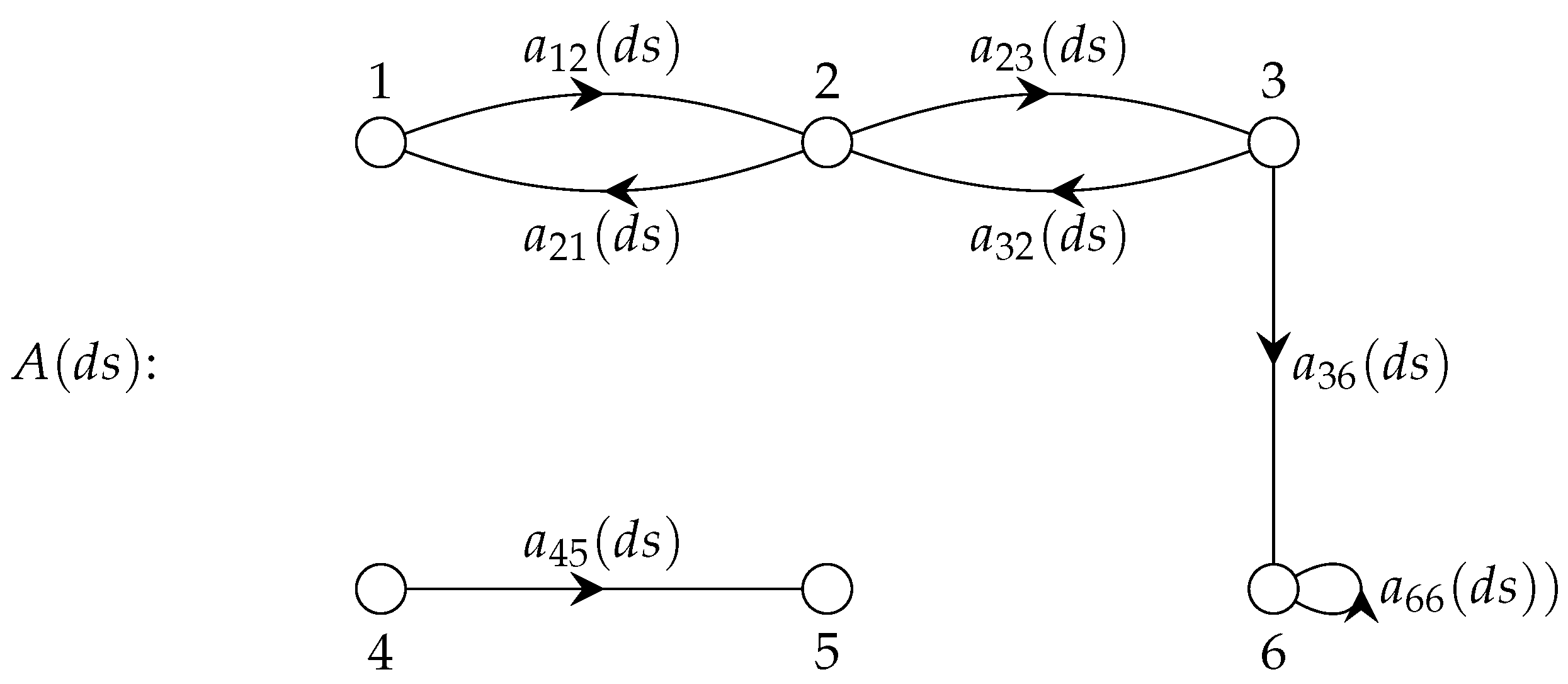
Example 3.

To illustrate the results, we consider the RFDE weighted loop-digraph shown in Figure 5.

The kernel matrix $A(ds)$ is

$$A(ds)=\begin{array}{cc}\begin{array}{ccc}& & \end{array}& \begin{array}{cccccc}& & & & & \end{array}\\ \begin{array}{ccc}& & \end{array}& \begin{array}{cccccc}{v}_1& v_2& v_3& v_4& v_5& v_6\end{array}\\ \begin{array}{ccc}& v_1& \\ & v_2\\ & v_3& \\ & v_4& \\ & v_5& \\ & v_6& \end{array}& \begin{array}{cccccc}0& a_{12}& 0& 0& 0& 0\\ a_{21}& 0& a_{23}& 0& 0& 0\\ 0& a_{32}& 0& 0& 0& a_{36}\\ 0& 0& 0& 0& a_{45}& 0\\ 0& 0& 0& 0& 0& 0\\ 0& 0& 0& 0& 0& a_{66}\end{array}\\ \begin{array}{ccc}& & \end{array}& \begin{array}{cccccc}& & & & & \end{array}\end{array},$$

(95)

where the dummy variable (ds) is suppressed within the matrix to reduce clutter.

The symmetric kernel matrix $A^S(ds)$ is

$$A^S(ds)=\begin{array}{cc}\begin{array}{ccc}& & \end{array}& \begin{array}{cccccc}& & & & & \end{array}\\ \begin{array}{ccc}& & \end{array}& \begin{array}{cccccc}{v}_1& v_2& v_3& v_4& v_5& v_6\end{array}\\ \begin{array}{ccc}& v_1& \\ & v_2\\ & v_3& \\ & v_4& \\ & v_5& \\ & v_6& \end{array}& \begin{array}{cccccc}0& a_{12}+a_{21}& 0& 0& 0& 0\\ a_{12}+a_{21}& 0& a_{23}+a_{32}& 0& 0& 0\\ 0& a_{23}+a_{32}& 0& 0& 0& a_{36}\\ 0& 0& 0& 0& a_{45}& 0\\ 0& 0& 0& a_{45}& 0& 0\\ 0& 0& a_{36}& 0& 0& 2^{·}{a}_{66}\end{array}\\ \begin{array}{ccc}& & \end{array}& \begin{array}{cccccc}& & & & & \end{array}\end{array}.$$

(96)

The reachability matrix $R$ is

$$R=\begin{array}{cc}\begin{array}{ccc}& & \end{array}& \begin{array}{cccccc}& & & & & \end{array}\\ \begin{array}{ccc}& & \end{array}& \begin{array}{cccccc}{v}_1& v_2& v_3& v_4& v_5& v_6\end{array}\\ \begin{array}{ccc}& v_1& \\ & v_2\\ & v_3& \\ & v_4& \\ & v_5& \\ & v_6& \end{array}& \begin{array}{cccccc}1& 1& 1& 0& 0& 1\\ 1& 1& 1& 0& 0& 1\\ 1& 1& 1& 0& 0& 1\\ 0& 0& 0& 1& 1& 0\\ 0& 0& 0& 0& 1& 0\\ 0& 0& 0& 0& 0& 1\end{array}\\ \begin{array}{ccc}& & \end{array}& \begin{array}{cccccc}& & & & & \end{array}\end{array}.$$

(97)

The transpose reachability matrix $R^T$ is

$$R^T=\begin{array}{cc}\begin{array}{ccc}& & \end{array}& \begin{array}{cccccc}& & & & & \end{array}\\ \begin{array}{ccc}& & \end{array}& \begin{array}{cccccc}{v}_1& v_2& v_3& v_4& v_5& v_6\end{array}\\ \begin{array}{ccc}& v_1& \\ & v_2\\ & v_3& \\ & v_4& \\ & v_5& \\ & v_6& \end{array}& \begin{array}{cccccc}1& 1& 1& 0& 0& 0\\ 1& 1& 1& 0& 0& 0\\ 1& 1& 1& 0& 0& 0\\ 0& 0& 0& 1& 0& 0\\ 0& 0& 0& 1& 1& 0\\ 1& 1& 1& 0& 0& 1\end{array}\\ \begin{array}{ccc}& & \end{array}& \begin{array}{cccccc}& & & & & \end{array}\end{array}.$$

(98)

The symmetric reachability matrix $R^S$ is

$$R^S=\begin{array}{cc}\begin{array}{ccc}& & \end{array}& \begin{array}{cccccc}& & & & & \end{array}\\ \begin{array}{ccc}& & \end{array}& \begin{array}{cccccc}{v}_1& v_2& v_3& v_4& v_5& v_6\end{array}\\ \begin{array}{ccc}& v_1& \\ & v_2\\ & v_3& \\ & v_4& \\ & v_5& \\ & v_6& \end{array}& \begin{array}{cccccc}1& 1& 1& 0& 0& 1\\ 1& 1& 1& 0& 0& 1\\ 1& 1& 1& 0& 0& 1\\ 0& 0& 0& 1& 1& 0\\ 0& 0& 0& 1& 1& 0\\ 1& 1& 1& 0& 0& 1\end{array}\\ \begin{array}{ccc}& & \end{array}& \begin{array}{cccccc}& & & & & \end{array}\end{array}.$$

(99)

This yields the weak components $\{v_1,v_2,v_3,v_6\}$ and $\{v_4,v_5\}$.

The element-wise product reachability matrix $R\times R^T$ is

$$R\times R^T=\begin{array}{cc}\begin{array}{ccc}& & \end{array}& \begin{array}{cccccc}& & & & & \end{array}\\ \begin{array}{ccc}& & \end{array}& \begin{array}{cccccc}{v}_1& v_2& v_3& v_4& v_5& v_6\end{array}\\ \begin{array}{ccc}& v_1& \\ & v_2\\ & v_3& \\ & v_4& \\ & v_5& \\ & v_6& \end{array}& \begin{array}{cccccc}1& 1& 1& 0& 0& 0\\ 1& 1& 1& 0& 0& 0\\ 1& 1& 1& 0& 0& 0\\ 0& 0& 0& 1& 0& 0\\ 0& 0& 0& 0& 1& 0\\ 0& 0& 0& 0& 0& 1\end{array}\\ \begin{array}{ccc}& & \end{array}& \begin{array}{cccccc}& & & & & \end{array}\end{array}.$$

(100)

This yields the strong components $\{v_1,v_2,v_3\}$, $\{v_4\}$, $\{v_5\}$, and $\{v_6\}$.

The connectedness matrix C is given by

$$C=\begin{array}{cc}\begin{array}{ccc}& & \end{array}& \begin{array}{cccccc}& & & & & \end{array}\\ \begin{array}{ccc}& & \end{array}& \begin{array}{cccccc}{v}_1& v_2& v_3& v_4& v_5& v_6\end{array}\\ \begin{array}{ccc}& v_1& \\ & v_2\\ & v_3& \\ & v_4& \\ & v_5& \\ & v_6& \end{array}& \begin{array}{cccccc}3& 3& 3& 0& 0& 2\\ 3& 3& 3& 0& 0& 2\\ 3& 3& 3& 0& 0& 2\\ 0& 0& 0& 3& 2& 0\\ 0& 0& 0& 2& 3& 0\\ 2& 2& 2& 0& 0& 3\end{array}\\ \begin{array}{ccc}& & \end{array}& \begin{array}{cccccc}& & & & & \end{array}\end{array}.$$

(101)

By applying the appropriate permutation matrix or simply interchanging the rows of columns of the kernel matrix $A(ds)$ in accordance with the weak components, the kernel matrix is expressed in decomposed form, as follows:

The kernel matrix $A(ds)$ is

$$A(ds)=\begin{array}{cc}\begin{array}{ccc}& & \end{array}& \begin{array}{cccccc}& & & & & \end{array}\\ \begin{array}{ccc}& & \end{array}& \begin{array}{cccccc}{v}_1& v_2& v_3& v_6& v_4& v_5\end{array}\\ \begin{array}{ccc}& v_1& \\ & v_2\\ & v_3& \\ & v_6& \\ & v_4& \\ & v_5& \end{array}& \begin{array}{cccccc}0& a_{12}& 0& 0& 0& 0\\ a_{21}& 0& a_{23}& 0& 0& 0\\ 0& a_{32}& 0& a_{36}& 0& 0\\ 0& 0& 0& a_{66}& 0& 0\\ 0& 0& 0& 0& 0& a_{45}\\ 0& 0& 0& 0& 0& 0\end{array}\\ \begin{array}{ccc}& & \end{array}& \begin{array}{cccccc}& & & & & \end{array}\end{array}.$$

(102)

The kernel matrix $A(ds)$ is expressed succinctly in the decomposed form

$$A(ds)=\left[\begin{array}{cc}{A}_{11}(ds)& O_{4\times 2}\\ O_{2\times 4}& A_{22}(ds)\end{array}\right],$$

(103)

where $A_{11}(ds)$ and $A_{22}(ds)$ are respectively $4\times 4$ and $2\times 2$ kernel matrices, and $O_{2\times 4}$ and $O_{4\times 2}$ are respectively $2\times 4$ and $4\times 2$ zero matrices.

The fundamental solution $\Phi (t)$ can be expressed in decomposed form

$$\Phi (t)=\left[\begin{array}{cc}{\Phi }_{11}(t)& O_{4\times 2}\\ O_{2\times 4}& {\Phi }_{22}(t)\end{array}\right],$$

(104)

where ${\Phi }_{11}(t)$ and ${\Phi }_{22}(t)$ are respectively the fundamental solutions for the kernel matrices $A_{11}(ds)$ and $A_{22}(ds)$.

4. Characteristics of Fundamental Solution

4.1. Fundamental Solution is Laplace Inverse of Resolvent Matrix

The fundamental solution satisfies the Volterra integro-differential equation of convolutional type

$${\Phi }^{\prime }(t)=\underset{0}{\overset{t}{\int }}A(ds)\Phi (t-s),t>0,\Phi (0)=I.$$

(105)

Taking the Laplace transform, we have

$$\begin{array}{cc}\hfill z\widehat{\Phi }(z)-I& =\widehat{\Phi }(z)\left[\underset{0}{\overset{a}{\int }}A(ds)e^{-zs}\right]\hfill \end{array}$$

(106)

$$\begin{array}{cc}\hfill \Delta (z)\widehat{\Phi }(z)& =I\hfill \end{array}$$

(107)

$$\begin{array}{cc}\hfill \widehat{\Phi }(z)& ={\Delta }^{-1}(z)\hfill \end{array}$$

(108)

$$\begin{array}{cc}\hfill \Phi (t)& ={\mathcal{L}}^{-1}\left({\Delta }^{-1}(z)\right).\hfill \end{array}$$

(109)

Consequently, the fundamental solution is the Laplace inverse of the resolvent matrix ${\Delta }^{-1}(z)$. Alternatively, the Laplace transform of the fundamental solution $\Phi (t)$ is the resolvent matrix ${\Delta }^{-1}(z)$.

4.2. Tauberian Behavior

From the previous subsection, we have

$$\widehat{\Phi }(z)=\underset{0}{\overset{\infty }{\int }}\Phi (t)exp(-zt)dt={\Delta }^{-1}(z)={\left(zI-\underset{0}{\overset{a}{\int }}A(ds)exp(-zs)\right)}^{-1}.$$

(110)

Assume that all the characteristic roots of the characteristic determinant $det(\Delta (z))$ have real part less than zero, so that ${\alpha }_0<0$. Choose $\alpha$ so that ${\alpha }_0<\alpha$. Then $\Phi (t)exp(-\alpha t)$ is integrable and we have

$$\underset{0}{\overset{\infty }{\int }}\Phi (t)exp(-\alpha t)dt={\left(\alpha I-\underset{0}{\overset{a}{\int }}A(ds)exp(-\alpha s)\right)}^{-1}$$

(111)

In particular for $\alpha =0$ we have

$$\underset{0}{\overset{\infty }{\int }}\Phi (t)dt={\left(-\underset{0}{\overset{a}{\int }}A(ds))\right)}^{-1}.$$

(112)

4.3. Contour Integral Version of Fundamental Solution

Let us consider the expression for the fundamental solution ${\Phi }_{ci}(t)$ in the form of Laplace inverse as a contour integral in the z-plane

$${\Phi }_{ci}(t)=\frac{1}{2\pi i}{\int }_{(c)}{e}^{zt}{\Delta }^{-1}(z)dz=\frac{1}{2\pi i}{\int }_{(c)}{e}^{zt}\frac{\mathrm{adj}(\Delta (z))}{det(\Delta (z))}dz.$$

(113)

For notational convenience, we put $C(z)=\mathrm{adj}(\Delta (z))$, $D(z)=det(\Delta (z))$, and $E(z)=1/det(\Delta (z))$.

To obtain the contribution to the integral of a characteristic root ${\lambda }_r$ of $det(\Delta (\lambda ))=0$ with multiplicity $m_r$, we consider the integral over a small circle centered at ${\lambda }_r$ containing no other characteristic roots of $det(\Delta (\lambda ))=0$.

Following the approach in Reference [10], we have

$$\begin{array}{cc}\hfill e^{zt}& =e^{{\lambda }_{r}t}{e}^{(z-{\lambda }_r)t}=e^{{\lambda }_{r}t}\sum _{n=0}\frac{t^n}{n!}{(z-{\lambda }_r)}^n,\hfill \end{array}$$

(114)

$$\begin{array}{cc}\hfill C(z)& =\sum _{n=0}\frac{1}{n!}{C}^{(n)}({\lambda }_r){(z-{\lambda }_r)}^n,\hfill \end{array}$$

(115)

$$\begin{array}{cc}\hfill D(z)& ={(z-{\lambda }_r)}^{m_r}\sum _{n=0}\frac{1}{(n+m_r)!}{D}^{((n+m_r))}({\lambda }_r){(z-{\lambda }_r)}^n.\hfill \end{array}$$

(116)

We have that $E(z)$, the reciprocal function of $D(z)$, is given by

$$E(z)={(z-{\lambda }_r)}^{-m_r}\sum _{n=0}{E}_n({\lambda }_r){(z-{\lambda }_r)}^n,$$

(117)

where $E_0({\lambda }_r)=m_r!/D^{((m_r))}({\lambda }_r)$, and $E_n({\lambda }_r)$ for $n\ge 1$ is obtained recursively from

$$\sum _{m=0}^n\frac{1}{(m+m_r)!}{E}_{n-m}({\lambda }_r)D^{((m+m_r))}({\lambda }_r)=0.$$

(118)

We have

$$e^{zt}{\Delta }^{-1}(z)=e^{{\lambda }_{r}t}{(z-{\lambda }_r)}^{-m_r}\sum _{k_1=0k_2=0k_3=0}^{\infty }\frac{t^{k_1}}{k_1!k_2!}{C}^{(k_2)}({\lambda }_r)E_{k_3}({\lambda }_r){(z-{\lambda }_r)}^{k_1+k_2+k_3}.$$

(119)

The residue for the characteristic root ${\lambda }_r$ is the coefficient of ${(z-{\lambda }_r)}^{-1}$ corresponding to $k=k_1+k_2+k_3=m_r-1$. It is given by

$$e^{{\lambda }_{r}t}\sum _{k_1+k_2+k_3=m_r-1}\frac{t^{k_1}}{k_1!k_2!}{C}^{(k_2)}({\lambda }_r)E_{k_3}({\lambda }_r){(z-{\lambda }_r)}^{k_1+k_2+k_3}.$$

(120)

The matrix coefficient ${\Psi }_{rj}$ is given by

$${\Psi }_{rj}=\frac{1}{j!}\sum _{k_2+k_3=m_r-1-j}\frac{1}{k_2!}{C}^{(k_2)}({\lambda }_r)D_{k_3}({\lambda }_r).$$

(121)

For example ${\Psi }_{r,m_r-1}=C({\lambda }_r)m_r/D^{(m_r)}({\lambda }_r)$, and for $m_r=1$${\Psi }_{r,0}=C({\lambda }_r)/D^{\prime }({\lambda }_r)$.

We have arrived at the following theorem:

Theorem 10.

Let $\{{\lambda }_r\}$ be the characteristic roots of the characteristic determinant $det(\Delta (z))=0$ with multiplicity $m_r$. The version of the fundamental solution ${\Phi }_{ci}(t)$ arising from a contour integral has the form of spectral decomposition of exponential solutions

$${\Phi }_{ci}(t)=\sum _r\sum _{j=0}^{m_r-1}{\Psi }_{rj}{t}^{j}exp({\lambda }_{r}t),$$

(122)

where

$${\Psi }_{rj}=\frac{1}{j!}\sum _{k_2+k_3=m_r-1-j}\frac{1}{k_2!}{C}^{(k_2)}({\lambda }_r)E_{k_3}({\lambda }_r).$$

(123)

In the case that all characteristic roots ${\lambda }_r$ are simple with multiplicity $m_r=1$ we have

$${\Phi }_{ci}(t)=\sum _r{\Psi }_{r}exp({\lambda }_{r}t),$$

(124)

where ${\Psi }_r=C({\lambda }_r)/D^{\prime }({\lambda }_r)$. For the scalar case $n=1$, $C(z)\equiv 1$ so that ${\Psi }_r=1/D^{\prime }({\lambda }_r)$.

Example 4.

Consider

$$\begin{array}{cc}\hfill x_1^{{}^{\prime }}(t)& =A_1{x}_2(t-a)\hfill \end{array}$$

(125)

$$\begin{array}{cc}\hfill x_2^{{}^{\prime }}(t)& =A_2{x}_3(t-a)\hfill \end{array}$$

(126)

$$\begin{array}{cc}\hfill x_3^{{}^{\prime }}(t)& =0.\hfill \end{array}$$

(127)

$$A(ds)=\left[\begin{array}{ccc}0& A_1\delta (s-a)& 0\\ 0& 0& A_2\delta (s-a)\\ 0& 0& 0\end{array}\right].$$

(128)

$$A^2(ds)=\left[\begin{array}{ccc}0& 0& A_1{A}_2\delta (s-2a)\\ 0& 0& 0\\ 0& 0& 0\end{array}\right].$$

(129)

$A^n(ds)=0$ for $n\ge 3$ so that $A(ds)$ is a nilpotent matrix with index 3. The weighted loop-digraphs for the kernel matrix and its convolutional powers for the RFDE are shown in Figure 6.

The fundamental matrix $\Phi (t)$ is

$$\Phi (t)=\left[\begin{array}{ccc}H(t)& A_1{(t-a)}_{+}& \frac{1}{2}{A}_1{A}_2{(t-2a)}_{+}^2\\ 0& H(t)& A_2{(t-a)}_{+}\\ 0& 0& H(t)\end{array}\right].$$

(130)

$$\Delta (z)=\left[\begin{array}{ccc}z& -A_1{e}^{-za}& 0\\ 0& z& -A_2{e}^{-za}\\ 0& 0& z\end{array}\right].$$

(131)

$$C(z)=\left[\begin{array}{ccc}{z}^2& A_{1}z{e}^{-za}& A_1{A}_2{e}^{-2za}\\ 0& z^2& A_{2}z{e}^{-za}\\ 0& 0& z^2\end{array}\right].$$

(132)

$D(z)=z^3$.

The contribution to the contour integral is

$$\sum _{k_1+k_2=2}\frac{t^{k_1}}{k_1!k_2!}{C}^{(k_2)}(0)=\frac{1}{2}{C}^{(2)}(0)+t{C}^{(1)}(0)+\frac{1}{2}{t}^{2}C(0).$$

(133)

The contour integral version of the fundamental solution ${\Phi }_{ci}(t)$ is given by

$${\Phi }_{ci}(t)=\left[\begin{array}{ccc}1& A_1(t-a)& \frac{1}{2}{A}_1{A}_2{(t-2a)}^2\\ 0& 1& A_2(t-a)\\ 0& 0& 1\end{array}\right].$$

(134)

Note for this specific example that ${\Phi }_{ci}(t)\equiv \Phi (t)$ for $t\ge 2a$, but that ${\Phi }_{ci}(t)\ne \Phi (t)$ for $0\le t<2a$. As this example has only a finite number of terms in ${\Phi }_{ci}(t)$ and $\Phi (t)$, convergence is not a factor in the discrepancy. The issue is that $\Phi (t)$ is compelled to contain truncated powers of t to reflect delay activations, whereas by its nature ${\Phi }_{ci}(t)$ is compelled to contain untruncated powers of t.

An open question is to characterize the minimum time $t_0$ for the equality of ${\Phi }_{ci}(t)$ and $\Phi (t)$ given by $t_0={inf}_{\tau >-a}\{\tau ;{\Phi }_{ci}(t)\equiv \Phi (t)\mathrm{for}t>\tau \}$. The matter has been encountered and considered in the literature (see References [6,7,8,9]) with values of $t_0$ ranging from $-a$ to $na$.

4.4. Semigroup Relations

The fundamental solution $\Phi (t)$ for the ODE $x^{\prime }(t)=Ax(t)$ satisfies the semigroup relation $\Phi (t_1+t_2)=\Phi (t_1)\Phi (t_2)$. The generalization for the fundamental solution $\Phi (t)$ for an RFDE

$$x^{\prime }(t)=\underset{0}{\overset{a}{\int }}A(ds)x(t-s)$$

(135)

is as follows:

Theorem 11.

For $t_1\geqq 0$ and $t_2\geqq 0$

$$\Phi (t_1+t_2)=\Phi (t_1)\Phi (t_2)+\underset{-a}{\overset{0}{\int }}d\alpha \underset{-\alpha }{\overset{a}{\int }}\left[ds\right]\Phi (t_1-s-\alpha )A(ds)\Phi (t_2+\alpha ).$$

(136)

Proof. 

This follows from the representation of the solution with $f=0$ and the consideration that the translate of a solution of an autonomous linear RFDE is also a solution. □

Remark 7.

A related result is found in Reference [24].

Remark 8.

It follows from the representation of solutions that the double integral has the following equivalent forms (see Equation (58)):

$$\begin{array}{}\hfill \mathrm{(137)}& \begin{array}{cc}\hfill \underset{-a}{\overset{0}{\int }}d\alpha \underset{-\alpha }{\overset{a}{\int }}A(ds)\Phi (t-s-\alpha )\Phi (t_2+\alpha )& =\underset{-a}{\overset{0}{\int }}d\alpha \underset{-\alpha }{\overset{a}{\int }}\left[ds\right]\Phi (t-s-\alpha )A(ds)\Phi (t_2+\alpha )\hfill \end{array}\hfill \hfill \mathrm{(138)}& \begin{array}{cc}\hfill & =\underset{0}{\overset{a}{\int }}\left[ds\right]\underset{-s}{\overset{0}{\int }}d\alpha \Phi (t-s-\alpha )A(ds)\Phi (t_2+\alpha )\hfill \end{array}\hfill \hfill \mathrm{(139)}& \begin{array}{cc}\hfill & =\underset{0}{\overset{a}{\int }}\left[ds\right]\underset{-s}{\overset{0}{\int }}d\alpha A(ds)\Phi (t-s-\alpha ))\Phi (t_2+\alpha ).\hfill \end{array}\hfill \end{array}$$

4.5. Semigroup of Solution Operators

In this subsection we consider the role played by the fundamental solution $\Phi (t)$ in solution operators mapping the initial function h to the solution $x(t;h)$ in the function spaces $M^2([-a,0],{\mathbb{R}}^n)$ and $C([-a,0],{\mathbb{R}}^n)$.

The solution $x(t;h)$ is given by

$$\begin{array}{}\hfill \mathrm{(140)}& \begin{array}{cc}\hfill x(t;h)& =\Phi (t)h(0)+\underset{-a}{\overset{0}{\int }}d\alpha \underset{-\alpha }{\overset{a}{\int }}A(ds)\Phi (t-s-\alpha )h(\alpha )\hfill \end{array}\hfill \hfill \mathrm{(141)}& \begin{array}{cc}\hfill & =\Phi (t)h(0)+\underset{-a}{\overset{0}{\int }}d\alpha \tilde{\Phi }(t,\alpha )h(\alpha ),\hfill \end{array}\hfill \end{array}$$

where

$$\begin{array}{cc}\hfill \tilde{\Phi }(t,\alpha )& =\underset{-\alpha }{\overset{a}{\int }}A(ds)\Phi (t-s-\alpha ).\hfill \end{array}$$

(142)

Remark 9.

Note that a solution operator has to accommodate two aspects of the initial function h: (i) the initial value $h(0)$ acted on by the fundamental solution $\Phi (t)$, and (ii) the initial function h as an integrand with kernel $\tilde{\Phi }(t,\alpha )$.

For the function space $M^2([-a,0],{\mathbb{R}}^n)={\mathbb{R}}^n\times L^2([-a,0],{\mathbb{R}}^n)$ we use the notation $\overline{h}=(h(0),h)$ and ${\overline{x}}_t(h)=(x(t;h),x_t(h))$, where

$$x_t(h)(\theta )=x(t+\theta ;h),-a\le \theta \le 0.$$

(143)

The $M^2([-a,0],{\mathbb{R}}^n)$ solution operator $S(t)$ is given by

$$\begin{array}{cc}\hfill S(t)\overline{h}& ={\overline{x}}_t(\overline{h})\hfill \end{array}$$

(144)

$$\begin{array}{cc}\hfill S(t)(h(0),h)& =(x(t;h),x_t(h)).\hfill \end{array}$$

(145)

We write

$$S(t)(h(0),h)=\left[\begin{array}{cc}{S}_{00}(t)h(0)& S_{01}(t)h\\ S_{10}(t)h(0)& S_{11}(t)h\end{array}\right],$$

(146)

where

$$\begin{array}{cc}\hfill S_{00}(t)& :{\mathbb{R}}^n\to {\mathbb{R}}^n,S_{00}(t)h(0)=\Phi (t)h(0),\hfill \end{array}$$

(147)

$$\begin{array}{cc}\hfill S_{01}(t)& :L^2\to {\mathbb{R}}^n,S_{01}(t)h=\underset{-a}{\overset{0}{\int }}d\alpha \tilde{\Phi }(t,\alpha )h(\alpha ),\hfill \end{array}$$

(148)

$$\begin{array}{cc}\hfill S_{10}(t)& :{\mathbb{R}}^n\to L^2,(S_{10}(t)h(0))(\theta )=\Phi (t+\theta )h(0),\hfill \end{array}$$

(149)

$$\begin{array}{cc}\hfill S_{11}(t)& :L^2\to L^2,(S_{11}(t)h)(\theta )=\underset{-a}{\overset{0}{\int }}d\alpha \tilde{\Phi }(t+\theta ,\alpha )h(\alpha ).\hfill \end{array}$$

(150)

The $C([-a,0],{\mathbb{R}}^n)$ solution operator $T(t)$ is given by

$$\begin{array}{cc}\hfill T(t)h& =x_t(h)\hfill \end{array}$$

(151)

$$\begin{array}{}\hfill \mathrm{(152)}& \begin{array}{cc}\hfill (T(t)h)(\theta )& =x(t+\theta ;h)\hfill \end{array}\hfill \hfill \mathrm{(153)}& \begin{array}{cc}\hfill & =\Phi (t+\theta )h(0)+\underset{-a}{\overset{0}{\int }}d\alpha \tilde{\Phi }(t+\theta ,\alpha )h(\alpha ).\hfill \end{array}\hfill \end{array}$$

The solution operator $S(t)$ on the function space $M^2([-a,0],{\mathbb{R}}^n)$ is a strongly continuous semigroup of linear operators for $t\ge 0$ satisfying: (i) $S(0)=I$, (ii) $S(t_1+t_2)=S(t_1)S(t_2)$ for $t_1,t_2\ge 0$, and (iii) ${lim}_{t\downarrow 0}\parallel S(t)h-h\parallel =0$. See References [22,25,26,27]. Likewise for the solution operator $T(t)$ on the function space $C([-a,0],{\mathbb{R}}^n)$. See References [8,13,15].

4.6. Picard Iteration

Definition 8.

The $n^{th}$ Picard iteration $\{{\Phi }_n(t)\}$ for the fundamental solution $\Phi (t)$ based on its Volterra integral equation $\Phi (t)=I+\underset{0}{\overset{t}{\int }}B(s)\Phi (t-s)ds$ is

$${\Phi }_0(t)=I,{\Phi }_{n+1}(t)=I+\underset{0}{\overset{t}{\int }}B(s){\Phi }_n(t-s)ds.$$

(154)

Theorem 12.

The $n^{th}$ Picard iteration ${\Phi }_n(t)$ is given by

$$\begin{array}{}\hfill \mathrm{(155)}& \begin{array}{cc}\hfill {\Phi }_n(t)& =I+{\displaystyle \sum _{j=1}^n}\underset{0}{\overset{t}{\int }}{B}^j(s)ds\hfill \end{array}\hfill \hfill \mathrm{(156)}& \begin{array}{cc}\hfill & ={\displaystyle \sum _{j=0}^n}\frac{1}{j!}\underset{0}{\overset{t}{\int }}{A}^j(ds){(t-s)}^j.\hfill \end{array}\hfill \end{array}$$

Proof. 

Arguing by induction, it suffices to show that

$$\underset{0}{\overset{t}{\int }}dsB(s)\underset{0}{\overset{t-s}{\int }}{B}^n(u)=\underset{0}{\overset{t}{\int }}ds\underset{0}{\overset{s}{\int }}duB(s-u)B^n(u)=\underset{0}{\overset{t}{\int }}ds{B}^{n+1}(s).$$

(157)

The first equation in the proof follows from a change in dummy integration variables, and the second from the definition of $B^n(s)$. The second equation in the theorem follows from $\underset{0}{\overset{t}{\int }}{B}^n(s)ds=\frac{1}{n!}\underset{0}{\overset{t}{\int }}{A}^n(ds){(t-s)}^n$. □

5. Extensions to other Functional Differential Equations

5.1. p-th Order RFDE

We consider fundamental solution $\Phi (t)$ for the p-th order RFDE with n-vector $x(t)$

$$x^{(p)}=\underset{0}{\overset{a}{\int }}A(ds)x(t-s).$$

(158)

By the standard procedure we convert the p-th order RFDE for n-vector $x(t)$ into a first order RFDE for a $pn$-vector $y(t)$

$$y^{\prime }(t)=\underset{0}{\overset{a}{\int }}\mathcal{A}(ds)y(t-s),$$

(159)

where the $pn\times pn$ companion matrix $\mathcal{A}(ds)$ is given by

$$\mathcal{A}(ds)=\left[\begin{array}{ccccc}0& I_n\delta (s)& 0& \cdots & 0\\ 0& 0& I_n\delta (s)& \cdots & 0\\ \cdots & \cdots & \cdots & \cdots & \cdots \\ A(ds)& 0& 0& \cdots & 0\end{array}\right].$$

(160)

The $pn\times pn$ fundamental solution is $\Phi (t)=({\Phi }_{ij}(t))$ where

$${\Phi }_{ij}(t)=\sum _{m=0}^{\infty }\frac{1}{(pm+k)!}\underset{0}{\overset{t}{\int }}{A}^{m+l}(ds){(t-s)}^{pm+k},$$

(161)

where

$$k=\left\{\begin{array}{cc}j-i,\hfill & \mathrm{if}j\ge i,\hfill \\ j+p-1,\hfill & \mathrm{if}j<i,\hfill \end{array}\right.\mathrm{and}l=\left\{\begin{array}{cc}1,\hfill & \mathrm{if}i>j,\hfill \\ 0,\hfill & \mathrm{if}i\le j.\hfill \end{array}\right.$$

(162)

In particular, for $p=2$

$$\Phi (t)=\left[\begin{array}{cc}{\Phi }_{11}(t)& {\Phi }_{12}(t)\\ {\Phi }_{21}(t)& {\Phi }_{22}(t)\end{array}\right],$$

(163)

where

$$\begin{array}{cc}\hfill {\Phi }_{11}(t)& ={\Phi }_{22}=\sum _{n=0}^{\infty }\frac{1}{2n!}\underset{0}{\overset{t}{\int }}{A}^n(ds){(t-s)}^{2n},\hfill \end{array}$$

(164)

$$\begin{array}{cc}\hfill {\Phi }_{12}(t)& =\sum _{n=0}^{\infty }\frac{1}{(2n+1)!}\underset{0}{\overset{t}{\int }}{A}^n(ds){(t-s)}^{2n+1},\hfill \end{array}$$

(165)

$$\begin{array}{cc}\hfill {\Phi }_{21}(t)& =\sum _{n=0}^{\infty }\frac{1}{(2n+1)!}\underset{0}{\overset{t}{\int }}{A}^{n+1}(ds){(t-s)}^{2n+1}.\hfill \end{array}$$

(166)

See Reference [28].

5.2. Infinite Delay

The RDFE with finite delay has a kernel matrix $A(ds)\in {\mathbb{B}}_{cs}^{+}$ with compact support and an initial function space defined over a finite interval $[-a,0]$. In contrast, the RDFE with infinite (or unbounded) delay has a kernel matrix with non-compact support and an initial function space defined on the infinite interval $(-\infty ,0]$. There is a wide variety of choices for this initial function space and the theory for the RDFE with infinite delay is intricately intertwined with a choice (see Reference [29]). However, the fundamental solution, with its simple initial condition of $\Phi (0)=I$ and $\Phi (t)=O$ for $t<0$ is exempt from these intricacies.

Reference [29] considers the fundamental solution for the equation

$$x^{\prime }(t)=\sum _{j=0}^{\infty }{A}_{j}x(t-{\theta }_j)+\underset{0}{\overset{t}{\int }}A(t-s)x(s)ds,t>0,$$

(167)

where $0={\theta }_0<{\theta }_1<\cdots <{\theta }_N<\cdots$, ${\sum }_{j=0}^{\infty }\left|\right|A_j\left|\right|<\infty$, and $\left|\right|A(s)\left|\right|\in L^1[0,\infty )$. We assume that there is no finite accumulation point and that there is some minimum separation $\alpha ={inf}_i({\theta }_{i+1}-{\theta }_i)>0$, so that given $0<T<\infty$ we can find N so that ${\theta }_N\le T<{\theta }_{N+1}$.

For tractability we split Equation (167) into two equations corresponding to discrete delays and a distributed delay, as follows:

$$x^{\prime }(t)=\sum _{j=0}^{\infty }{A}_{j}x(t-{\theta }_j),t>0,$$

(168)

and

$$x^{\prime }(t)=\underset{0}{\overset{t}{\int }}A(t-s)x(s)ds,t>0.$$

(169)

The fundamental solutions for Equation (168) for $t\in (0,T]$ is

$$\Phi (t)=I+\sum _{r_0+\cdots +r_N=n=1}^{\infty }\frac{1}{r_0!\cdots r_N!}{A}_0^{r_0}\cdots A_N^{r_N}{(t-r_0{\theta }_0-\cdots -r_N{\theta }_N)}_{+}^n.$$

(170)

In this expression we assume either (i) we are dealing with the scalar case or (ii) that the matrices $A_0\cdots A_N$ commute. Note that for fixed t we have a finite sum if $A_0=0$. The method of steps for computing the fundamental solution $\Phi (t)$ will work in this case.

The fundamental solutions for Equation (169) is

$$\Phi (t)=\sum _{n=0}^{\infty }\frac{1}{n!}\underset{0}{\overset{t}{\int }}{A}^n(s){(t-s)}^{n}ds,t>0.$$

(171)

It is possible, as demonstrated in the following example, that in the case of an infinite delay that the fundamental solution satisfies an ODE—without a delay.

Example 5.

Consider the scalar case with $A(t)=exp(-Kt){\sum }_{i=0}^p{a}_i{t}^i$ so that

$$x^{\prime }(t)=\underset{0}{\overset{t}{\int }}\left\{\sum _{i=0}^p{a}_i{(t-s)}^i\right\}exp(-K(t-s))x(s)ds,t>0.$$

(172)

Multiplying Equation (172) by $exp(Kt)$, differentiating $p+1$ times, and then multiplying by $exp(-Kt)$, we obtain that the fundamental solution $\Phi (t)$ satisfies the ${(p+2)}^{th}$ order ODE

$$\sum _{j=0}^{p+1}\left(\genfrac{}{}{0pt}{}{p+1}{j}\right)K^j{x}^{((p+2-j))}(t)=\sum _{j=0}^p{K}^j\sum _{i=0}^{p-j}i!a_i{x}^{((p-j-i))}(t).$$

(173)

Consequently the fundamental solution satisfies an ODE with no delay.

5.3. Nonautonomous RFDE

We consider the fundamental solution $\Phi (t,s)$ for the nonautonomous RFDE

$$x^{\prime }(t)=\underset{s}{\overset{t}{\int }}{d}_{\tau }A(t,\tau )x(\tau ),t>s,$$

(174)

where $A(t,\tau )$ is measurable in t, of bounded variation in $\tau$ for $s<\tau <t$, constant for $\tau \ge t$, and

$$\underset{s}{\overset{T}{\int }}dt|\underset{s}{\overset{T}{\int }}{d}_{\tau }A(t,\tau )|<\infty .$$

(175)

The fundamental solution $\Phi (t,s)$ (also known as the Cauchy function $C(t,s)$) satisfies initial conditions $\Phi (s,s)=I$, and $\Phi (t,s)=O$ for $t<s$.

We integrate to obtain the equivalent Volterra integral equation

$$\Phi (t,s)=I+\underset{s}{\overset{t}{\int }}d{\tau }_1\underset{s}{\overset{{\tau }_1}{\int }}{d}_{{\tau }_2}A({\tau }_1,{\tau }_2)\Phi ({\tau }_2,s).$$

(176)

Applying Picard iteration, we obtain the fundamental solution $\Phi (t,s)$ in the form

$$\Phi (t,s)=I+\sum _{n=1}^{\infty }\underset{s}{\overset{t}{\int }}d{\tau }_1\underset{s}{\overset{{\tau }_1}{\int }}{d}_{{\tau }_2}A({\tau }_1,{\tau }_2)\cdots \underset{s}{\overset{{\tau }_{2n-2}}{\int }}d{\tau }_{2n-1}\underset{s}{\overset{{\tau }_{2n-1}}{\int }}{d}_{{\tau }_{2n}}A({\tau }_{2n-1},{\tau }_{2n}).$$

(177)

Note that in the autonomous case that the Picard iteration for the fundamental solution of the nonautonomous RFDE reduces to the established expression

$$\Phi (t)=\sum _{n=0}^{\infty }\frac{1}{n!}\underset{0}{\overset{t}{\int }}{A}^n(ds){(t-s)}^n.$$

(178)

6. Conclusions

This paper has extended the expression for and the treatment of the fundamental solution for autonomous linear RFDE from scalar to n-vector, in the following ways: The fundamental solution is presented in the form of a convolutional exponential matrix function. The paper demonstrates how RFDE analysis can be conducted through an interplay of the RFDE actors (fundamental solution, kernel matrix, characteristic matrix, characteristic determinant, resolvent matrix) and tools (Laplace transform and solution representation). Elements of algebraic graph theory are applied in the form of a weighted loop-digraph to illuminate the system structure and dynamics, and to identify the strong and weak components. This is potentially a powerful tool in the case that the RFDE has a special structure, such as coupled oscillators with delay interactions. The paper compares the fundamental solution $\Phi (t)$ of an RFDE with its contour integral version ${\Phi }_{ci}(t)$ for a special example, and raises an open question on the minimum time $t_0$ for equivalence. For $t>t_0$, ${\Phi }_{ci}(t)$ plays the role of a spectral representation for the fundamental solution $\Phi (t)$. In its explicit form and in tandem with the solution representation, the paper describes the key role played by the fundamental solution in the semigroup of solution operators. The paper considers the fundamental solution for other functional differential equations (p-th order RFDE, RFDE with infinite delay, nonautonomous RFDE), but stops short of Neutral and Partial functional differential equations. Finally, the paper opens the door to future work on fundamental solutions and associated analysis for (i) RFDEs with a special structure and (ii) Neutral and Partial functional differential equations.

References

- McCalla, C. Exact Solutions of Some Functional Differential Equations. In An International Symposium; Cesari, L., Hale, J.K., LaSalle, J.P., Eds.; Academic Press: New York, NY, USA, 1976; Volume 2, pp. 163–168. [Google Scholar]
- McCalla, C. Zeros of the Solutions of First Order Functional Differential Equations. SIAM J. Math. Anal. 1978, 9, 843–847. [Google Scholar] [CrossRef]
- McCalla, C. Asymptotic Behavior of First Order Scalar Linear Autonomous Retarded Functional Differential Equations. Funct. Differ. Equ. 2018, 25, 155–187. [Google Scholar]
- Coddington, E.A.; Levinson, N. The Theory of Ordinary Differential Equations; Robert E. Krieger Publishing Co.: Malabar, India, 1983. [Google Scholar]
- Doetsch, G. Introduction to the Theory and Applications of the Laplace Transform; Springer: New York, NY, USA, 1974. [Google Scholar]
- Banks, H.T.; Manitius, A. Projection Series for Retarded Functional Differential Equations with Applications to Optimal Control Problems. J. Differ. Equ. 1975, 18, 296–332. [Google Scholar] [CrossRef] [Green Version]
- Bellman, R.; Cooke, K.L. Differential-Difference Equations; Academic Press: New York, NY, USA, 1963. [Google Scholar]
- Verduyn Lunel, S.M. Exponential Type Calculus for Linear Delay Equations; Centre for Mathematics and Computer Science, Tract No. 57, Amsterdam 1989; Springer: New York, NY, USA, 1993. [Google Scholar]
- Verduyn Lunel, S.M. Series Expansions and Small Solutions for Volterra Equations of Convolution Type. J. Differ. Equ. 1995, 85, 17–53. [Google Scholar] [CrossRef] [Green Version]
- Levinson, N.; McCalla, C. Completeness and Independence of the Exponential Solutions of Some Functional Differential Equations. Stud. Appl. Math. 1974, 53, 1–15. [Google Scholar] [CrossRef]
- Gripenberg, G.; Londen, S.-O.; Staffans, O. Volterra Integral and Functional Equations; Cambridge University Press: Cambridge, UK, 1990. [Google Scholar]
- Myshkis, A.D. Linear Differential Equations with Retarded Arguments; Nauka: Moscow, Russia, 1972. [Google Scholar]
- Hale, J.K.; Verduyn Lunel, S.M. Introduction to Functional Differential Equations; Springer: New York, NY, USA, 1993. [Google Scholar]
- Diekmann, O.; Gils, S.A.; Verduyn Lunel, S.M.; Walther, H.-O. Delay Equations, Functional-, Complex-, and Nonlinear Analysis; Springer: New York, NY, USA, 1995. [Google Scholar]
- Kappel, F. Linear Autonomous Functional Differential Equations. In Delay Equations and Applications; Arino, O., Hbid, M.L., Ait Dads, E., Eds.; Springer: Dordrecht, The Netherlands, 2006; pp. 41–139. [Google Scholar]
- Azbelev, N.V.; Maksimov, V.P.; Rakhmatullina, L.F. Introduction to the Theory of Functional Differential Equations: Methods and Applications; Hindawi Publishing Corporation: New York, NY, USA, 2007. [Google Scholar]
- Vlasov, V.V.; Medvedev, D.A. Functional-Differential Equations in Sobolev Spaces and Related Problems of Spectral Theory. J. Math. Sci. 2010, 64, 659–841. [Google Scholar] [CrossRef]
- Agarwal, R.; Berezansky, L.; Braverman, E.; Domoshnitsky, A. Nonoscillation Theory of Functional Differential Equation with Applications; Springer: New York, NY, USA, 2012. [Google Scholar]
- Horn, R.A.; Johnson, C.R. Matrix Analysis, 2nd ed.; Cambridge University Press: New York, NY, USA, 2013. [Google Scholar]
- Kappel, F. Laplace-Transform Methods and Linear Autonomous Functional-Differential Equations; Bericht Nr. 64, Mathematisch-Statistischen Sektion in Forschungszentrum Graz: Graz, Austria, 1976. [Google Scholar]
- Hartman, P. Ordinary Differential Equations; Philip Hartman: Baltimore, MD, USA, 1973. [Google Scholar]
- Delfour, M.C.; Mitter, S.K. Hereditary Differential Equations with Constant Delays II—A Class of Affine Systems and the Adjoint Problem. J. Differ. Equ. 1975, 18, 399–409. [Google Scholar] [CrossRef] [Green Version]
- Harary, F.; Norman, R.Z.; Cartwright, D. Structural Models: An Introduction to the Theory of Directed Graphs; John Wiley & Sons: New York, NY, USA, 1965. [Google Scholar]
- Richardson, J.M. Quasi-Differential Equations and Generalized Semigroup Relations. J. Math. Anal. Appl. 1961, 2, 293–298. [Google Scholar] [CrossRef] [Green Version]
- Bernier, C.; Manitius, A. On Semigroups in Rn × Lp corresponding to Differential Equations with Delays. Can. J. Math. 1978, 30, 897–914. [Google Scholar] [CrossRef]
- Delfour, M.C.; Manitius, A. The Structural Operator F and its Role in the Theory of Retarded Systems, I. J. Math. Anal. Appl. 1980, 73, 359–381. [Google Scholar] [CrossRef] [Green Version]
- Delfour, M.C.; Manitius, A. The Structural Operator F and its Role in the Theory of Retarded Systems, II. J. Math. Anal. Appl. 1980, 75, 466–490. [Google Scholar] [CrossRef] [Green Version]
- McCalla, C. Oscillatory and Asymptotic Behavior of Second Order Functional Differential Equations. Nonlinear Anal. Theory Methods Appl. 1979, 3, 283–291. [Google Scholar] [CrossRef]
- Corduneanu, C.; Lakshmikantham, V. Equations with Unbounded Delay: A Survey. Nonlinear Anal. Theory Methods Appl. 1980, 4, 831–877. [Google Scholar] [CrossRef] [Green Version]
Figure 1.
Relationships between retarded functional differential equation (RFDE) actors.
Figure 2.
Weighted loop-digraph for general RFDE.
Figure 3.
Weighted loop-digraphs for Example 1.
Figure 4.
Weighted loop-digraphs for Example 2.
Figure 5.
Weighted loop-digraph for Example 3.
Figure 6.
Weighted loop-digraphs for Example 4.
© 2020 by the author. Licensee MDPI, Basel, Switzerland. This article is an open access article distributed under the terms and conditions of the Creative Commons Attribution (CC BY) license (http://creativecommons.org/licenses/by/4.0/).
Share and Cite
MDPI and ACS Style
McCalla, C. On Fundamental Solution for Autonomous Linear Retarded Functional Differential Equations. Mathematics 2020, 8, 1418. https://0-doi-org.brum.beds.ac.uk/10.3390/math8091418
AMA Style
McCalla C. On Fundamental Solution for Autonomous Linear Retarded Functional Differential Equations. Mathematics. 2020; 8(9):1418. https://0-doi-org.brum.beds.ac.uk/10.3390/math8091418
Chicago/Turabian StyleMcCalla, Clement. 2020. "On Fundamental Solution for Autonomous Linear Retarded Functional Differential Equations" Mathematics 8, no. 9: 1418. https://0-doi-org.brum.beds.ac.uk/10.3390/math8091418
Note that from the first issue of 2016, this journal uses article numbers instead of page numbers. See further details here.