An Evolutionary Approach to Improve the Halftoning Process
by
 , , , and
Noé Ortega-Sánchez
1 ,
,
Diego Oliva
1,2,* ,
,
Erik Cuevas
1 ,
,
Marco Pérez-Cisneros
1,* and
Angel A. Juan
2
1
División de Electrónica y Computación, Universidad de Guadalajara, CUCEI, Av. Revolución 1500, Guadalajara CP. 44430, Jal, Mexico
2
IN3-Computer Science Department, Universitat Oberta de Catalunya, 08860 Castelldefels, Spain
*
Authors to whom correspondence should be addressed.
Mathematics 2020, 8(9), 1636; https://0-doi-org.brum.beds.ac.uk/10.3390/math8091636
Submission received: 14 August 2020
/
Revised: 17 September 2020
/
Accepted: 18 September 2020
/
Published: 22 September 2020
(This article belongs to the Special Issue Evolutionary Image Processing)
Abstract
:The techniques of halftoning are widely used in marketing because they reduce the cost of impression and maintain the quality of graphics. Halftoning converts a digital image into a binary image conformed by dots. The output of the halftoning contains less visual information; a possible benefit of this task is the reduction of ink when graphics are printed. The human eye is not able to detect the absence of information, but the printed image stills have good quality. The most used method for halftoning is called Floyd-Steinberger, and it defines a specific matrix for the halftoning conversion. However, most of the proposed techniques in halftoning use predefined kernels that do not permit adaptation to different images. This article introduces the use of the harmony search algorithm (HSA) for halftoning. The HSA is a popular evolutionary algorithm inspired by the musical improvisation. The different operators of the HSA permit an efficient exploration of the search space. The HSA is applied to find the best configuration of the kernel in halftoning; meanwhile, as an objective function, the use of the structural similarity index (SSIM) is proposed. A set of rules are also introduced to reduce the regular patterns that could be created by non-appropriate kernels. The SSIM is used due to the fact that it is a perception model used as a metric that permits comparing images to interpret the differences between them numerically. The aim of combining the HSA with the SSIM for halftoning is to generate an adaptive method that permits estimating the best kernel for each image based on its intrinsic attributes. The graphical quality of the proposed algorithm has been compared with classical halftoning methodologies. Experimental results and comparisons provide evidence regarding the quality of the images obtained by the proposed optimization-based approach. In this context, classical algorithms have a lower graphical quality in comparison with our proposal. The results have been validated by a statistical analysis based on independent experiments over the set of benchmark images by using the mean and standard deviation.
1. Introduction
In the industrial processes, it is always necessary to look for an enhancement in the products or reduce costs. In a simple word, the resources should be optimized to provide the best experience to the customer. Enterprises usually employ publicity to increase the number of sales. Some transmission media are radio, television, magazines, newspapers, and recently digital alternatives related to the internet. However, the printing stills are the alternative used on a large scale. Halftoning is a tool used to transform a digital image into a dotted binary image. The idea is to compress the frequency of the tones independently if the image is in grayscale or color space. The resultant image possesses different dots that conform to the continues-tones. This image contains less visual information that is not perceived by the human eye due to the blurring effects [1]. Then, the aim of halftoning can be summarized in the creation of an image with fewer amplitude levels that can be perceptually similar to the original [2].
Different printing devices take advantage of halftoning, and it is included as a step that permits the reduction of resources such as ink [3]. Ink reduction is a common implementation, and it happens due to the print devices having a limited color palette. Halftoning has been extensively used, for example, in newspapers where the output binary values are a representation of blank ink or spaces [1]. It has also been applied in digital typesetters, medical instruments, and scientific devices [4]. The importance of halftoning is not only for printing but also for the transmission of information and representation [5]. It is necessary to develop an accurate halftoning mechanism to increase the quality of the output images; it helps, for example, to reduce the waste of ink in printing devices [3]. The strengths and weaknesses of halftoning algorithms are discussed in the present work; also introduced here is an alternative method that can obtain better results with desired characteristics.
In the related literature, it is possible to find different halftoning algorithms, and they can be classified into three categories: (1) Ordered dither, (2) error diffusion, and (3) patterning [6]. The algorithms considered in the article are based on the error diffusion; it is the most used approach with a reserved performance due to the fact that the same kernel is applied in all the images. The most outstanding representative method is called Floyd-Steinberger [7], although it is not the only one. It has been widely used and compared with the algorithm proposed by Jarvis, Judice, and Ninke [8], and with the method introduced by Stucki and Sierra [9]. The main drawback of these techniques is that the error diffusion kernel is assumed to be known a priori. The assumption that all images can be treated with the same kernel becomes impractical since each image has its unique characteristics.
On the other hand, from the best of our knowledge, the use of metaheuristic algorithms (MA) that include the evolutionary methods has not been proposed for halftoning. MA are important tools used to solve complex optimization problems [10,11]. Some examples of their use are in data classification [12] and medical diagnosis [13,14]. In this paper, an alternative approach to calculating a personalized kernel based on the features of the image is presented. The best kernel computation is then treated as an optimization problem. The harmony search algorithm (HSA) is a MA that was used widely in the last years to solve complex optimization problems with high performance and accuracy. Since the publication of HSA in [15], it has been adapted in applications such as vanishing point detection [16], block matching for motion estimation [17], phase optimization of wavefront shaping [18], etc. The virtues of HSA are a straightforward implementation, good convergence, and low computational cost. Similar to other MA, the HSA has a metaphor that it is related to musical improvisation. In other words, the search procedure consists of the exploration of a search space looking for the best solution using operators that imitate the improvisation of new melodies. The algorithm has a memory that stores different harmonies; then, in the iterative process, a new harmony can be selected from the memory or randomly created. When a harmony is taken from the memory, it can also be adjusted. It means that the candidate solution is perturbated to verify if a better harmony exists around it. Finally, the worst element of the memory is replaced if the new harmony has a better objective function value.
For the halftoning process, the HSA is used to estimate the best parameters of a kernel. In this sense, each harmony is considered as a kernel that is applied to generate a binary output image. In the iterative process, the fitness (objective function) is the structural similarity index (SSIM) [19] that permits checking if the elements of the new image are similar to the original. The experimental results quantitatively show that the implementation based on HSA has values slightly higher than the standard procedures of halftoning. The methods used for comparisons are Jarvis-Judice-Ninke [8], Floyd-Steinberg [7], Sierra-Dithering [2], and Stucki [9]. The peak signal-noise-to-ratio (PSNR) and SSIM are employed to compare the quality of images of all the methods [20].
The main contribution of this article is the proposal of an adaptive method for halftoning. In the proposed approach, a unique kernel for each image is estimated; this is possible since our algorithm considers halftoning as an optimization problem. By computing an adaptive kernel, it is possible to preserve the best features of the input image and create more visually detailed outputs. To enhance the accuracy the use of the HSA to identify the best values for each index is introduced. This optimization process considers the SSIM as a criterion of evaluation due to its capabilities to compare two digital images. In addition, to avoid the computation of kernels that produce regular patterns, it is proposed based on the HSA and different design rules to obtain the internal values of the kernel. By using this version, the randomness permits avoiding the regular patterns, but also the quality of the output images is enhanced.
The remainder of the paper is organized as follows: Section 2 offers the related work of different algorithms of halftoning and the metaheuristic algorithm HSA. Section 3 presents the approach to solve the halftoning with HSA. Section 4 demonstrates the experimental results and discussion to illustrate the effectiveness of the proposed method. Finally, Section 5 shows a conclusion of the use of personalized kernels based on the HSA.
2. Preliminaries
2.1. Halftoning
Image processing halftoning is a process commonly used to compress the information contained in the image. This fact permits printing or displaying the image in different formats. An example of the use of halftoning is a publication by offset printing, such as in newspapers, magazines, and books. This kind of offset is most used in the industry to reach a large-scale audience. With the use of dots to form objects in images, it is possible to fool the perception and show different levels of gray [6] (see Figure 1). This fact occurs due to grouping and the distance between the dots. Based on the previous statement, is it necessary to find the best representation of the images with the use of dots.
The related literature has representative algorithms for halftoning in digital images. To understand their behavior, we would analyze approaches to create an image with dots. In this sense, the output of such methods will be an image that fools the human perception.
The process of halftoning is carried out through the image following a trajectory from top to bottom and from left to right. During this procedure, the pixels are evaluated with a kernel. The aim is to distribute the error since the pixels that are binarized generate an accumulative error [21]. The error is distributed between its lower and left neighborhoods; the graphical representation of this procedure is shown in Figure 2.
In this way, when evaluating the pixel of interest, it will become 0 or 255, depending on the cut-off value [2,22], and the distribution error in the neighborhood amortizes its difference. It is a simple process, and it can generate competitive results and enhance quality.
Halftoning Algorithms
The definition of halftoning is the visual representation of the “noise”. The halftoning is commonly described as a process used to generate an image in terms of noise called dither, but the results are not aligned with the spatial dither. The dither is the error that has been decorrelated by adding random noise in the input. One of the side effects is that this method creates ghosts in the visual area of the resulting images.
Error diffusion: The error diffusion is a popular halftoning technique (Equation (1)); it assumes a given image of size in grayscale. The treatment of each pixel in this approach is from top to down and from left to right. In this process, the feedback is not considered in the pixels already treated. Here, and denote the original pixel value and the output result of error diffusion, respectively, where and .
From Equation (1), m and n are the indexes for rows and columns in the image. Meanwhile, denotes the selected kernel. Initially, a value associated with the current grayscale pixel value is compared with the threshold . In other words, the error-diffused greyscale value is computed. If is smaller than the threshold , the output of the error is 255. Equation (2) describes how to calculate the values of eij and bij.
Floyd-Steinberg: The Floyd-Steinberg approach proposed in [7] is a technique that has the advantage of not presenting any ghosting effect, and the output is computed in a parallel way. However, it tends to blur the image; therefore, a visual appreciation is not accurate for the human expert. The kernel generates an output image with a delicate texture, low contrast, and some artifacts tend to dissipate into the output image. The kernel proposed in the Floyd-Steinberg method is described in Equation (3).
Jarvis-Judice-Ninke: The algorithm of Jarvis-Judice-Ninke [8] has the virtue to obtain a high contrast output. One of the problems of this method is that the texture of the halftone image is rough. Moreover, it was proposed in the 70s. The technique is also based on the error diffusion and possesses a kernel of 12-coefficients as presented in Equation (4).
A kernel with the same dimensions was also introduced by Stucki [9], and it has a larger filter used to reduce directional artifacts (Equation (5)).
Sierra Dithering: The last studied algorithm for halftoning is called Sierra Dithering [23]. This method employs a simple filter that produces better results than the original Floyd-Steinberg filter. The kernel of the Sierra Dithering approach is presented in Equation (6).
2.2. Harmony Search Algorithm
The harmony search algorithm (HSA) was developed in an analogy with the music improvisation process, where music players improvise the pitches of their instruments to obtain a better harmony [24]. In this sense, one of the advantages is that the HSA is easy to codify. It works using a harmony, which represents a solution that exists in an n-dimensional space. A harmony is saved in the harmony memory (HM); then, a new solution could be created from two possible ways: (1) Randomly generated, always between the limits of the problem, and (2) by selecting a harmony from HM to compose a new solution. The possibility of adjusting or to improve the new candidate solution takes into consideration the pitch adjustment rate (PAR) operation. At this stage, a bandwidth (BW) that permits a fine adjustment is used. Finally, the last stage is the inclusion of the new harmony in the HM by using a rule that only allows updating if the fitness of the new harmony is better than the worst element of the HM. The basic HSA consists of three phases: HM initialization, improvisation of the new harmony, and updating of the HM. The HSA has shown excellent performance in diverse areas and applications [25].
The computational procedure of HSA is summarized as follows:
| Step 1: | Set the parameter HMS, HMCR, PAR, BW, and NI. |
| Step 2: | Initialize the HM and calculate the objective function value of each harmony. |
| Step 3: | Improvise a new harmony as follows: |
| for (j= 0 to d) do | |
| if (r1 < HMCR) then | |
| , where | |
| if (r2 < PAR) then | |
| , where | |
| end if | |
| if , then | |
| end if | |
| if , then | |
| end if | |
| else | |
| , where | |
| end if | |
| end for | |
| Step 4: | Update the HM as , if . |
| Step 5: | If NI is completed, the best harmony in the HM is returned; otherwise, go back to step 3. |
From the previous steps, d is the number of dimensions, upper() and lower() limit the boundaries of the search space. The r1, r2, r3 are random numbers uniformly distributed between 0 and 1. The use of random numbers is common in evolutionary algorithms because it permits diversifying the solutions by performing the exploration and exploitation of the search space.
3. Halftoning by Using Harmony Search Algorithm (HHSA)
Definition of the Optimization Problem
In general, halftoning could be addressed as an optimization problem; in this case, a kernel (the technique of halftoning) is optimized with the use of HSA to obtain a resultant image with enhanced quality in the contraposition of the other techniques of halftoning. Therefore, we treated the integration of the concepts of error diffusion into HSA and how it is possible to get an image with improved characteristics. The definition of the kernel has an essential role because the number of elements and the limits of each one is relevant to distribute the error.
On the HSA, a kernel is considered as harmony; in the execution of the algorithm, it makes a new configuration; as a result, it creates a new kernel. The first step is to calculate a harmony in random distribution between 1 and 10 (Equation (7)).
where and * are the pixels of interest.
The kernel is normalized, and with this action, the pixels in the neighborhood have a gradual increment. Therefore, the diffusion error is also distributed (see Figure 3). The possible values have been studied based on other algorithms, and we propose the boundaries of the search space in a range of 1 to 10; by this action, the kernel is optimized using the HSA. As shown in Figure 3, the kernel tours and creates a new image. The arrow’s direction indicates the kernel movement; the process is carried out with each new harmony.
The objective function considers the image obtained after applying the halftoning computed by the HHSA and the original image. After processing the image with the new kernel (), it is evaluated with Equation (8), resulting in a measure of similarity between the original image and the output. The new harmony is evaluated with SSIM (defined in Equation (9)) as a quality metric to improve in each iteration of our fitness, and it means that the objective function is the SSIM in the HHSA. The SSIM must be maximized to evaluate the quality of the solutions provided by the HHSA, due to the interrogative of how to evaluate an image.
The approach of this investigation uses the SSIM index (see Equation (9)) to measure the quality and similitude of images. Wang et al. developed it, and it is considered to be correlated with the quality perception of the human visual system (HVS) [19].
The elements evaluated in this Equation are divided into luminosity, contrast, and correlation; those components are fundamental for a proper comparison. The first indicates how similar or close the luminance is between the two images. The second evaluates the contrast and shows if the images are similar in this term. If the values are near 1 the images are closer. The last term is the comparison in structural forms, evaluating the correlation coefficient between f and g. The SSIM index throws values in the range of [0, 1]. The constant values are used to avoid a null denominator. The set of evaluations of the terms provides us with valuable information that is used as an objective function. As was previously mentioned, the SSIM is a maximization problem and considers the image obtained after applying the new kernel in each iteration. In this sense, a new image f (output of the kernel) is created and compared with the image g (original) and computed with Equation (8), but first, it would be proceeded to estimate the values of the kernel.
On the other hand, a comparative study is performed using the PSNR. The best solution obtained using the proposed HHSA is compared with the original image. Although the resultant images are impartial, at the same time, they prove the enhanced results. The PSNR is a metric in which its properties are used to evaluate an image; when the values tend to be zero, it means the quality of the image is accurate. Given a reference image f and a test image g, both sizes of M × N, and the PSNR between f and g is defined by:
In the case of getting higher PSNR values to indicate a higher image quality, in the other direction, we will expect a lower similitude between the images. In other words, the differences between the images are higher. Therefore, the images are different. Although PSNR is a metric that has stood out to compare images, it is only used to validate the HHSA results. In this way, the best kernel was already found, but the PSNR is used to verify the image quality.
4. Experimental Results
4.1. The Configuration of the HHSA
For the experiments performed, the parameters of HSA have been set as follows: HMS has 100 harmonies, HMCR is set in 0.7, and PAR has 0.3; the behavior of these last two parameters includes the exploration and the exploitation. It should be noted that these parameters are widely used and show excellent performance in state of the art. The NI was set in 1000; this number of iterations has been increased to ensure the convergence in our work. Moreover, it is possible to create rules in step 5 to stop the number of iterations, but in the experiments, we considered that it was better to leave a fixed number of iterations to find the optimal value. The parameters of HSA were set according to the guidelines provided in [15] and by considering some experiments.
The experimental results provide evidence of the performance of the proposed approach for the halftoning process; they were developed by different experiments with images of size 512 × 512. As explained in Section 3, the halftoning methodology and the HSA have been combined to get the optimal solution and proportionate the optimal customized kernel for each image; the proposed method is named HHSA. The images tested are commonly used as a benchmark in image processing. They have different degrees of complexity due to the elements contained in the scene. The set of benchmark images has twelve samples; some examples of the image used are presented in Figure 4. Simultaneously, a statistical test to prove the enhancement of the solutions has also been included. In this sense, the configuration settings of the algorithm have popular values that are widely used in the literature [25]. Moreover, different comparisons are developed into two ways, one for analytically verifying the quality of the solutions and the second to visually analyze the output of the algorithms where the human perspective is essential.
The Floyd–Steinberg filter, the Jarvis-Judice-Ninke, and the Stucki methods are used to measure the sensitivity of the SSIM and PSNR. We consider the proposed SSIM indexing approach as a particular implementation of structural similarity, from an image formation perspective. It is worth mentioning that PSNR is only used to evaluate the final results. With this, we perform a fair evaluation because it will not be the same metric with which the algorithm was run. The experiments are evaluated with SSIM and PSNR. The properties of SSIM are used as a measure of quality in the algorithms [26], where it is used to create a schema to select the neighborhood of the pixel. Some characteristics of SSIM that encourage using it in the proposed method are the following: Finding better values in luminance, contrast, and structure; finding the top ranking of the value gives an enhanced image [19]. On the other hand, the PSNR is used in the proposed approach to measure the output image from the HHSA, since it measures the quality of compression in reconstructed images. The metrics have a controversial role, and both have promoted variants [20]. However, they are widely used in the related literature.
4.2. Optimization Problem Results
When the HHSA is running, the fitness value has an interesting behavior, and the modification of the kernel generates a new candidate solution to obtain an image in halftones with better quality and perception. It is a fact that fitness changes as far as the kernel changes. In Figure 5, it is possible to see the results of running the proposal; in it, we show the first kernel and the last, and we could appreciate it. Previously, we wrote the speciation of HHSA, but one of the critical parameters is the thresholding of the halftoning in the test; practically, we established the value of 128.
Figure 6a shows how the best algorithm solution changes, and the kernel quality is improved. It is emphasized by the SSIM that is used to evaluate the quality of the solution. On the other hand, the changes of the worst vector solution are shown in Figure 6b; it is evident how the HSA memory is modified since it compares the new solutions with the worst one in the memory. From Figure 6a, it is possible to see that the algorithm converges around 700–800 iterations. However, the stop criterion is higher in order to provide a better perspective of the optimization.
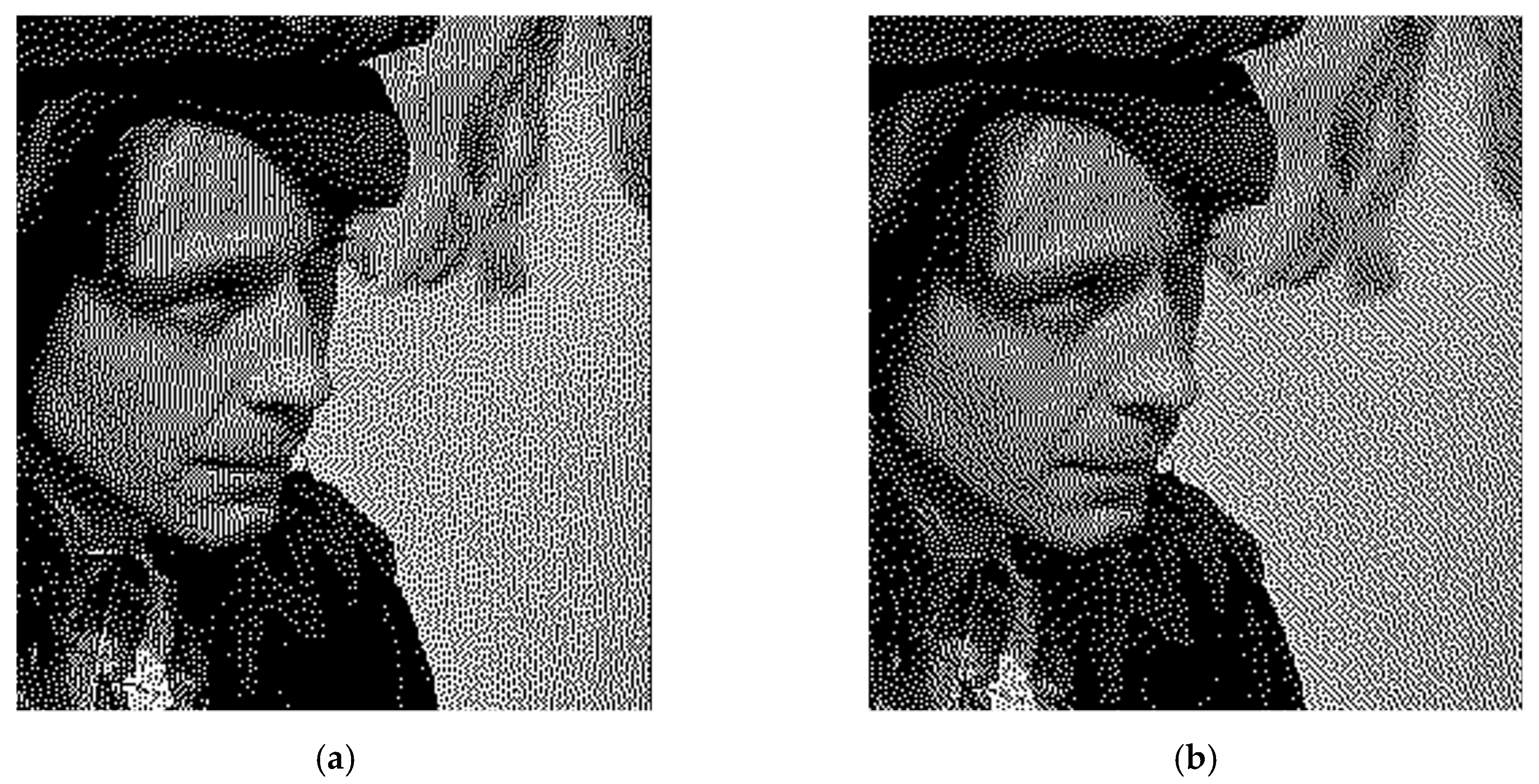
In Figure 7, different stages of maturity in the image are presented before obtaining the results. It is possible to analyze that Figure 7b has details near the nose, which are not aesthetic. Meanwhile, in Figure 7d, the nose looks detailed and presents more accuracy in the fur.
In Table 1, we show the statistical results, where the values of the HHSA are better in terms of SSIM and offer the same behavior with the PSNR. The proposed approach has notable performance in comparison with the classical algorithms of halftoning. In Table 1, it can be noted that the HHSA includes statistics since the study carried out a series of experiments with 35 independent runs. The reason is creating a validity study; it attracts the attention of the classical halftoning algorithms and does not have statistics since the kernel is fixed and, therefore, will always give the same value.
From the values in Table 1, it is appreciable that our proposal has advantages over the other halftoning algorithms. It made sense that the results have a significant difference, but in others, this advantage is less significant. This situation is not bad; it only confirms that our approach is competitive. From Table 1, it is possible to analyze that in all the cases, the HHSA provides a higher value in terms of SSIM; the second in the rank is the method called Jarvis-Judice-Ninke, and the worst is the Floyd-Steinberg approach. Notice that for this comparison, the mean of the SSIM for HHSA after 35 independent runs is considered. This value is taken to provide stability in the test in the execution of the algorithm. However, the standard deviation (std) in all the cases is lower. It means that the HHSA results are stable and do not vary from one iteration to another. Here, it is important to mention that the mean and std are not used for the other methods because they are not iterative. Regarding the PSNR, the proposed HHSA is a competitive alternative in most cases; it has a higher value. Meanwhile, the worst is from the Jarvis-Judice-Ninke approach.
On the other hand, Table 2 presents a comparative study that permits us to perform a visual inspection of the results and an appreciation between our algorithm and classical approaches. This table shows the 12 images used for the experiments and the results obtained by all the algorithms. From a visual inspection, it is possible to see that the outputs provided by HHSA possess more features related to the original image.
For a proper analysis of the results in Table 2, it is important to consider that the transmission of information into different media has some undesired effects; this paper presents a methodology using HSA and halftoning. A series of experiments were performed to validate the HHSA results. One of the main drawbacks of the halftoning version based on the HSA is that it creates regular patterns with low randomness. It occurs due to the nature of the optimization problem and because the HSA is searching for the best kernel that provides an output with a high similarity to the original image. This fact demerits the visual results of HHSA, especially when the images are loaded in a text file by reducing the size of the output. However, this affects the HHSA and the other dithering methodologies. The management of images in text processors has effects of losing quality when images are resized. To deal with the harmful effects, image processors have developed different formats trying not to lose quality. In this context, we have used image files with the extension .svg to overcome some failures, but even with this consideration, the output of our approach presents some not desired visual effects.
The images in Table 2 have some problems with the methods due to regular patterns created by the HHSA and the handling of the image files. Such issues came from the resizing and can be seen and analyzed by zooming the areas that present visual inconsistencies. For example, the images named test1, test2, test6, and test10 present not desired patterns, artifacts, and some sooty that is only present when the output images are resized. Thanks to the personalized kernel, each one has different behavior and presents some beneficial visual effects. To properly analyze the situations described above, in Figure 8b a zoom of the resultant image (test1) of Floyd-Steinberg’s method is presented. This image shows more patterns in the building in the background that is near fading away, in comparison to the output of the HHSA in Figure 8a, where the same objects are better defined and less blurred.
Other images from Table 2 present a high contrast due to the same situation of the low randomness in the patterns and the handling of the images in a text processor. However, for some halftoning methods, this situation does not occur. The computation of the output image by using an individually designed kernel obtained by the HHSA changes the frequency of the dots and affects the contrast of the output images. This fact is more notable in the images of test2, test5, test7, test9, and test12. Depending on the images that, in this case, are different optimization problems, the effects on the outputs could be more notorious. In this way, the results obtained by the HHSA are better and more details are defined from the objects of the scene. Some examples are presented in Figure 9, where the zoom and crop of some areas of test2 and test12 are presented for a visual inspection. In Figure 9a, the solid grayscale values of the input image are enhanced by using more dots. Meanwhile, some regions (mostly dark or white) do not require too many dots to define the objects. This fact occurs due to the personalized kernel (with regular patterns) created by the HHSA. In counterpart, Figure 9b shows the output provided by the Jarvis-Judice-Ninke method; from this sample, we can see that the regions as the hair is blurred and not well defined. This fact also occurs in the mirror, where some shadows are not properly represented. Regarding test12 and Figure 9c, the shapes in the sky and the object in the boat are clearly defined; it can be noticed due to the patterns created by the dots by using the kernel obtained by the HHSA. However, this behavior is not present in Figure 9d, which shows the output of the Floyd-Steinberg method. From this sample, we can see that the objects are not accurately defined, and the eye could lose some details between the points. The HHSA output is a good alternative for most of the images because it considers each of them as a unique problem. However, due to the nature of the problem, the solutions of the HHSA are optimal, and it does not mean that they are superior in most of the cases; of course, they could be improved, but as a prelaminar approach, it is competitive. In addition, the use of the computation of the unique kernel could help save resources in the printer and plot systems.
The regular patterns generated by the kernel could be good enough to recreate the images, but it is not desired. Moreover, handling the files has collateral effects; some of them are good, such as the enhanced transitions between structures. Some effects do not help with clarity, due to the stripes or patches in large areas without elements. The HHSA presents this drawback in some cases; it could be seen in Figure 10a. Furthermore, in Figure 10b it is less affected, but it could be seen that the stripes and the irregular dark pattern are more evident in some techniques.
4.3. Avoiding the Regular Patterns in HHSA
The study presented in Table 1 shows an improvement of the output images in terms of the SSIM and PSNR. In contrast, the images in Table 2 appear less competitive in comparison to the classical methods after applying the custom kernels. This occurs due to the process of finding the configuration of the kernel that generates regular patterns, and this causes a problem in the present images, even though the statistics show better values than the classical method. The HHSA calculates a custom kernel by looking for the best values based on the SSIM, and the quality is checked with the PSNR. However, it is well known in image processing that the value of a metric is not always the fair value compared to the image’s perception. This leads us to have images with the optimal SSIM and PSNR, but with low quality for human perception.
To overcome the problems previously explained, a series of additional experiments were performed to avoid the moiré effect [27] presented in some images. Therefore, a set of rules are also proposed and implemented in the HHSA in the pitch adjustment stage that will avoid this effect. It produces a new version called HHSA, avoiding regular patterns (HHSA-ARP). On the other hand, the values of the metrics (SSIM and PSNR) are lower than the first approach (see Table 3). However, it continues giving better values than the Floyd-Steinberg and the rest of the algorithms used for comparisons.
An attempt to solve the problem that creates regular pattern effects in the image consists of avoiding some configurations in the kernels (such as repeated numbers in the neighborhood). Then, in the HHSA an extra step in the pitch adjustment stage is included. This step helps verify if the kernel has a not desired configuration and computes new values for the elements of the matrix. The rules used in the HHSA-ARP are defined as follows:
The rules in Equation (12) were designed in consideration of the diffusion error that is made from left to right and from top to bottom. This has been done as an attempt to minimize the moiré effect; this effect is not desired, even though it has been used in other types of applications and benefits the investigations in other fields.
The new experiments throw a new series of statistics based on the implementation of the rules. They present a reduction in the SSSIM and PSNR values in contrast to the initial investigations, but they still are better than the other dithering methods. The output images show fewer effects of artifacts and regular patterns. We present the most representative images in Table 4, where it is the first attempt of HHSA, and the version of the HHSA configured to suppress the creation of regular patterns.
Table 4 presents samples from the set of benchmark images that were selected due to the effects of the regular patterns that are more comfortable to be visually identified. In the case of HHSA, the effect of the distortion due to regular patterns in the custom kernel are shown. The HHSA-ARP has the following characteristics: In test 1, a reduction of artifacts and other effects in the background of the sky can be seen, although the SSIM values have gone from 0.530965 to 0.52801318 and the PSNR values from 7.651838 to 7.622100038. In test2, it can be observed that the model’s face has been less affected by the moiré effect. For test4, the background on the right side is smooth, and the face of the pirate has fewer affectations. Finally, for test12 the benefits of the patterns created by adding the rules can be seen in the sky (especially in the upper left corner) and the back of the leading boat. Here, it is important to notice that the images are visually better, but the values of SSIM and PSNR suffer a reduction. It is evident because the nature of such metrics is a comparison pixel by pixel. However, they help provide a first approach that permits addressing the halftoning from an optimization point of view.
5. Conclusions
This article presents an implementation for halftoning based on the HSA called the HHSA. This method computes a personalized kernel for each image for halftoning. The proposed algorithm considers halftoning from an optimization point of view. In an iterative process, the HSA search for the best kernel configuration permits generating an optimal image based on dots. The idea is to create a unique kernel for each image using the SSIM as an objective function. The SSIM is proposed as an objective function because it permits comparing the input and output images based on the intrinsic information contained on them. In addition, a set of rules is also introduced that helps in having more accurate kernels that create visually better images, avoiding undesired artifacts in the output scene. Such rules are used in combination with the HSA and SSIM in a version called the HHSA-ARP.
The HHSA and HHSA-ARP can solve the disadvantages of classical methods regarding using only one kernel for all the images that do not permit the adaptation to complex images. The experimental results provide evidence that the HHSA and HHSA-ARP based halftoning approaches are an alternative for this purpose. In the comparisons, the HHSA-ARP provides competitive results to the classical approaches in terms of PSNR and SSIM. Moreover, the results were statistically validated to verify the stability of the HHSA and HHSA-ARP. In this way, the output images after applying the proposed algorithm are visually competitive with the obtained classical methods. However, it has points that it could be improved in future work. These improvements include developing specialized metrics for dithering images and implementing an objective function capable of reducing noise and extraneous patterns. In the case of the SSIM, it is possible to conclude that the results of the two proposed approaches outperformed the rest of the algorithms in the 12 benchmark images based on the statistics. Meanwhile, the output images in terms of the PSNR are compared to show that the results of the HSA based methods are improved in 11 of the 12 cases. Regarding the rest of the methods, the worst in terms of the SSIM is the Floyd-Steinberg and for PSNR the Jarvis-Judice-Ninke.
As future work, this methodology will be extended with other optimization algorithms considering different metrics. The presented approach also needs to be evaluated in images from different color spaces. In the same context, it is also necessary to study the influence of the threshold for halftoning. Furthermore, the use of multi-objective algorithms will also be explored.
Author Contributions
Conceptualization, N.O.-S., D.O., and E.C.; methodology, N.O.-S. and D.O.; software, N.O.-S.; validation, E.C., D.O., and M.P.-C.; formal analysis, N.O.-S., D.O., E.C., and A.A.J.; investigation, N.O.-S.; resources, N.O.-S., M.P.-C., and A.A.J.; data curation, E.C., M.P.-C., and A.A.J.; writing—original draft preparation, N.O.-S.; writing—review and editing, N.O.-S., D.O., and M.P.-C.; visualization, M.P.-C. and A.A.J.; supervision, D.O., E.C., M.P.-C. and A.A.J. All authors have read and agreed to the published version of the manuscript.
Funding
This research received no external funding.
Conflicts of Interest
The authors declare no conflict of interest.
References
- Crounse, K.R.; Chua, L.O.; Roska, T.; Roska, T. Image Halftoning with Cellular Neural Networks. IEEE Trans. Circuits Syst. II Analog Digit. Signal Process. 1993, 40, 267–283. [Google Scholar] [CrossRef]
- Ulichney, R. A Review of Halftoning Techniques. In Proceedings of the Color Imaging: Device-Independent Color, Color Hardcopy, and Graphic Arts V; SPIE: San Jose, CA, USA, 1999; Volume 3963, pp. 378–391. [Google Scholar]
- Jiang, W.; Veis, A.; Ulichney, R.; Allebach, J.P. Novel color halftoning algorithm for ink savings. Electron. Imaging 2018, 2018, 429-1–429-7. [Google Scholar] [CrossRef]
- Bakshi, A.; Patel, A.K. Halftoning Algorithm Using Pull-Based. In Proceedings of the International Conference on Innovative Computing and Communications; Lecture Notes in Networks and Systems; Bhattacharyya, S., Hassanien, A., Gupta, D., Khanna, A.P.I., Eds.; Springer: Singapore, 2019; pp. 411–419. [Google Scholar]
- Makarov, A.; Yakovleva, E. Comparative Analysis of Half toning Algorithms for Digital Watermarking. In Proceedings of the 18th Conference of Open Innovations Association and Seminar on Information Security and Protection of Information Technolog; IEEE: St. Petersburg, Russia, 2016; pp. 193–199. [Google Scholar]
- Lau, D.L.; Arce, G.R. Modern Digital Halftoning; CRC Press: Boca Raton, FL, USA, 2006; ISBN 9780471780496. [Google Scholar]
- Steinberg, R.W.; Floyd, L. An Adaptive Algorithm for Spatial Greyscale. Proc. Soc. 1976, 17, 75–77. [Google Scholar]
- Jarvis, J.F.; Judice, C.N.; Ninke, W.H. A survey of techniques for the display of continuous tone pictures on bilevel displays. Comput. Graph. image Process. 1976, 5, 13–40. [Google Scholar] [CrossRef]
- Stucki, P. Image processing for document reproduction. In Advances in digital image processing; Springer: Berlin/Heidelberg, Germany, 1979; pp. 177–218. [Google Scholar]
- Xu, Y.; Chen, H.; Luo, J.; Zhang, Q.; Jiao, S.; Zhang, X. Enhanced Moth-flame optimizer with mutation strategy for global optimization. Inf. Sci. (N. Y.) 2019, 492, 181–203. [Google Scholar] [CrossRef]
- Chen, H.; Heidari, A.A.; Chen, H.; Wang, M.; Pan, Z.; Gandomi, A.H. Multi-population differential evolution-assisted Harris hawks optimization: Framework and case studies. Futur. Gener. Comput. Syst. 2020, 111, 175–198. [Google Scholar] [CrossRef]
- Shen, L.; Chen, H.; Yu, Z.; Kang, W.; Zhang, B.; Li, H.; Yang, B.; Liu, D. Evolving support vector machines using fruit fly optimization for medical data classification. Knowl.-Based Syst. 2016, 96, 61–75. [Google Scholar] [CrossRef]
- Wang, M.; Chen, H.; Yang, B.; Zhao, X.; Hu, L.; Cai, Z.N.; Huang, H.; Tong, C. Toward an optimal kernel extreme learning machine using a chaotic moth-flame optimization strategy with applications in medical diagnoses. Neurocomputing 2017, 267, 69–84. [Google Scholar] [CrossRef]
- Wang, M.; Chen, H. Chaotic multi-swarm whale optimizer boosted support vector machine for medical diagnosis. Appl. Soft Comput. J. 2020, 88, 105946. [Google Scholar] [CrossRef]
- Geem, Z.W. Recent Advances in Harmony Search Algorithm; Springer: Berlin/Heidelberg, Germany, 2010; Volume 270. [Google Scholar]
- Moon, Y.Y.; Geem, Z.W.; Han, G.T. Vanishing point detection for self-driving car using harmony search algorithm. Swarm Evol. Comput. 2018, 41, 111–119. [Google Scholar] [CrossRef]
- Bhattacharjee, K.; Tiwari, A.; Kumar, S. Block Matching Algorithm Based on Hybridization of Harmony Search and Differential Evolution for Motion Estimation in Video Compression. In Soft Computing: Theories and Applications; Springer: Berlin/Heidelberg, Germany, 2018; pp. 625–635. [Google Scholar]
- Wu, Y.; Zhang, X.; Yan, H. Focusing light through scattering media using the harmony search algorithm for phase optimization of wavefront shaping. Opt. J. Light Electron Opt. 2018, 158, 558–564. [Google Scholar] [CrossRef]
- Wang, Z.; Bovik, A.C.; Sheikh, H.R.; Simoncelli, E.P. Image quality assessment: From error visibility to structural similarity. IEEE Trans. Image Process. 2004, 13, 600–612. [Google Scholar] [CrossRef] [PubMed] [Green Version]
- Horé, A.; Ziou, D. Image quality metrics: PSNR vs. SSIM. In Proceedings of the 20th International Conference on Pattern Recognition, Istabul, Turkey, 23–26 August 2010; pp. 2366–2369. [Google Scholar]
- Knuth, D.E. Digital halftones by dot diffusion. ACM Trans. Graph. 1987, 6, 245–273. [Google Scholar] [CrossRef]
- Ulichney, R.A. Dithering with blue noise. Proc. IEEE 1988, 76, 56–79. [Google Scholar] [CrossRef]
- Sierra, F. LIB 17. Proc. Dev.’s Den CIS Gr. Support Forum 1989. Unpublished. [Google Scholar]
- Geem, Z.W.; Kim, J.H.; Loganathan, G.V. A new heuristic optimization algorithm: Harmony search. Simulation 2001, 76, 60–68. [Google Scholar] [CrossRef]
- Ser, J.D. Harmony Search Algorithm: Proceedings of the 3rd International Conference on Harmony Search Algorithm (ICHSA 2017); Advances in Intelligent Systems and Computing; Springer: Singapore, 2017; ISBN 9789811037283. [Google Scholar]
- Wang, S.; Rehman, A.; Wang, Z.; Ma, S.; Gao, W. SSIM-motivated rate-distortion optimization for video coding. IEEE Trans. Circuits Syst. Video Technol. 2012, 22, 516–529. [Google Scholar] [CrossRef] [Green Version]
- Meadows, D.M.; Johnson, W.O.; Allen, J.B. Generation of Surface Contours by Moiré Patterns. Appl. Opt. 1970, 9, 942. [Google Scholar] [CrossRef] [PubMed]
Figure 1.
Cut out of image. (a) Original, (b) halftoning.

Figure 2.
An area of the image and the kernel trajectory.

Figure 3.
The cameraman (a) is processed with a kernel (c) in the arrow directions (b); after processing the image, it is evaluated with the structural similarity index (SSIM) to know the quality of the proposed kernel.
Figure 3.
The cameraman (a) is processed with a kernel (c) in the arrow directions (b); after processing the image, it is evaluated with the structural similarity index (SSIM) to know the quality of the proposed kernel.

Figure 4.
Samples of images to develop the test.

Figure 5.
Results of processing the original image (a), results of halftone with harmony search (HS) (b), and a cut and zoom of the boat (c,d).
Figure 5.
Results of processing the original image (a), results of halftone with harmony search (HS) (b), and a cut and zoom of the boat (c,d).

Figure 6.
Evolution of the fitness SSIM at each iteration. (a) The best particle of harmony memory (HM) (b) the worst harmony in the memory, which is a competition to new harmonies.
Figure 6.
Evolution of the fitness SSIM at each iteration. (a) The best particle of harmony memory (HM) (b) the worst harmony in the memory, which is a competition to new harmonies.

Figure 7.
The four different outputs of test3. (a) The fitness SSIM is low in Iteration 1 and shows defects and distortions. (b) The image is improved but still has some visual defects. We look at the values of fitness SSIM that are increasing. (c) The fitness SSIM almost reaches the optimal value but we let it keep iterating to find a better value. (d) The last fitness SSIM reaches a value which represents the best fitness and visualizes an image near the original image.

Figure 8.
A crop and zoom of image test1. (a) The output image after applying the proposed halftoning by using HSA (HHSA). (b) The output image after applying the method of Floyd-Steinberg. The zoom permits seeing dots and patterns in detail.
Figure 8.
A crop and zoom of image test1. (a) The output image after applying the proposed halftoning by using HSA (HHSA). (b) The output image after applying the method of Floyd-Steinberg. The zoom permits seeing dots and patterns in detail.

Figure 9.
A crop and zoom of image test2 and 12. (a) The output of image test2 after applying the proposed HHSA. (b) The output of image test2 after applying the method of Jarvis-Judice-Ninke. (c) The resultant image test12 after applying the proposed HHSA. (d) The output of image test12 after applying the method of Floyd-Steinberg. The zoom permits seeing dots and patterns in detail.

Figure 10.
A crop and zoom of image test4. (a) The output image after applying the proposed HHSA. (b) The output image after applying the method of Floyd-Steinberg. The zoom permits seeing artifacts and patterns in the face and background of the image.
Figure 10.
A crop and zoom of image test4. (a) The output image after applying the proposed HHSA. (b) The output image after applying the method of Floyd-Steinberg. The zoom permits seeing artifacts and patterns in the face and background of the image.


Table 1.
Statistical results.
| HHSA | Jarvis-Judice-Ninke | Floyd-Steinberg | Sierra-Dithering | Stucki | ||
|---|---|---|---|---|---|---|
| SSIM | ||||||
| mean | std | |||||
| test 1 | 0.530965 | 0.006110809 | 0.442754 | 0.305369 | 0.314663 | 0.378702 |
| test 2 | 0.483038 | 0.004577303 | 0.475290 | 0.280892 | 0.294486 | 0.380525 |
| test 3 | 0.584160 | 0.006311886 | 0.578918 | 0.371786 | 0.380374 | 0.454066 |
| test 4 | 0.611333 | 0.002879088 | 0.575283 | 0.449854 | 0.458353 | 0.511553 |
| test 5 | 0.485476 | 0.025799264 | 0.461556 | 0.313459 | 0.328122 | 0.368585 |
| test 6 | 0.470101 | 0.003897454 | 0.443539 | 0.277847 | 0.288033 | 0.358991 |
| test 7 | 0.544270 | 0.006003758 | 0.531579 | 0.323045 | 0.336291 | 0.426775 |
| test 8 | 0.487829 | 0.011720087 | 0.454227 | 0.269676 | 0.279263 | 0.356964 |
| test 9 | 0.583895 | 0.005794814 | 0.575704 | 0.401112 | 0.413867 | 0.474699 |
| test 10 | 0.519052 | 0.005425102 | 0.510012 | 0.29933 | 0.312307 | 0.401745 |
| test 11 | 0.548769 | 0.005214272 | 0.51432 | 0.366638 | 0.377768 | 0.418065 |
| test 12 | 0.495473 | 0.004611630 | 0.484349 | 0.314840 | 0.328805 | 0.400891 |
| PSNR | ||||||
| mean | std | |||||
| test 1 | 7.651838 | 0.034465888 | 7.228841 | 7.277824 | 7.270218 | 7.267355 |
| test 2 | 7.047287 | 0.086462267 | 6.697432 | 6.754390 | 6.746273 | 6.738812 |
| test 3 | 6.977601 | 0.040181257 | 6.659878 | 6.959343 | 6.93148 | 6.901012 |
| test 4 | 8.489320 | 0.065361811 | 8.020814 | 8.164862 | 8.14788 | 8.130009 |
| test 5 | 9.504212 | 0.037655832 | 7.539568 | 7.626550 | 7.614034 | 7.604983 |
| test 6 | 7.153715 | 0.040888407 | 6.841787 | 6.868554 | 6.864408 | 6.862674 |
| test 7 | 6.900233 | 0.056174709 | 6.628160 | 6.747999 | 6.735287 | 6.716799 |
| test 8 | 6.824300 | 0.028533137 | 6.582260 | 6.685023 | 6.675296 | 6.656737 |
| test 9 | 7.587587 | 0.069440544 | 7.058648 | 7.284244 | 7.262257 | 7.236547 |
| test 10 | 6.836581 | 0.052831395 | 6.593367 | 6.668213 | 6.660108 | 6.647340 |
| test 11 | 8.066916 | 0.081025465 | 7.419925 | 7.572861 | 7.551219 | 7.538850 |
| test 12 | 6.994021 | 0.037012217 | 6.689220 | 6.784387 | 6.774046 | 6.757137 |
Table 2.
Comparative between the resultant images of the different halftoning methods used in the experiments.
Table 2.
Comparative between the resultant images of the different halftoning methods used in the experiments.
| Original Image | HHSA | Floyd-Steinberg | Jarvis–Judice–Ninke | Sierra Dithering | Stucki | |
|---|---|---|---|---|---|---|
| test 1 |  |  |  |  |  |  |
| test 2 |  |  |  |  |  |  |
| test 3 |  |  |  |  |  |  |
| test 4 |  |  |  |  |  |  |
| test 5 |  |  |  |  |  |  |
| test 6 |  |  |  |  |  |  |
| test 7 |  |  |  |  |  |  |
| test 8 |  |  |  |  |  |  |
| test 9 |  |  |  |  |  |  |
| test 10 |  |  |  |  |  |  |
| test 11 |  |  |  |  |  |  |
| test 12 |  |  |  |  |  |  |
Table 3.
Comparative between HHSA and HHSA with rules to avoid regular patterns.
| SSIM | PSNR | |||||||
|---|---|---|---|---|---|---|---|---|
| HHSA | HHSA-ARP | HHSA | HHSA-ARP | |||||
| Mean | Std | Mean | Std | Mean | Std | Mean | Std | |
| test 1 | 0.530965 | 0.006110809 | 0.52801318 | 0.006915539 | 7.651838 | 0.034465888 | 7.622100038 | 0.042169674 |
| test 2 | 0.483038 | 0.004577303 | 0.47937723 | 0.005241727 | 7.047287 | 0.086462267 | 6.964648742 | 0.078500675 |
| test 3 | 0.584160 | 0.006311886 | 0.56332022 | 0.011727794 | 6.977601 | 0.040181257 | 6.949102235 | 0.066822314 |
| test 4 | 0.611333 | 0.002879088 | 0.60630796 | 0.006449049 | 8.489320 | 0.065361811 | 8.447737055 | 0.08213532 |
| test 5 | 0.485476 | 0.025799264 | 0.47840261 | 0.038499056 | 9.504212 | 0.037655832 | 8.612058266 | 0.775191246 |
| test 6 | 0.470101 | 0.003897454 | 0.46850974 | 0.005744441 | 7.153715 | 0.040888407 | 7.123846942 | 0.045259563 |
| test 7 | 0.544270 | 0.006003758 | 0.53583375 | 0.008759206 | 6.900233 | 0.056174709 | 6.848529485 | 0.041106374 |
| test 8 | 0.487829 | 0.011720087 | 0.4808898 | 0.008525419 | 6.824300 | 0.028533137 | 6.783413082 | 0.056248647 |
| test 9 | 0.583895 | 0.005794814 | 0.56849882 | 0.009178075 | 7.587587 | 0.069440544 | 7.496128991 | 0.078647944 |
| test 10 | 0.519052 | 0.005425102 | 0.51467182 | 0.00873848 | 6.836581 | 0.052831395 | 6.819108727 | 0.078024087 |
| test 11 | 0.548769 | 0.005214272 | 0.54609907 | 0.546099069 | 8.066916 | 0.081025465 | 8.010846971 | 0.049816626 |
| test 12 | 0.495473 | 0.004611630 | 0.49094678 | 0.004913998 | 6.994021 | 0.037012217 | 6.918520971 | 0.066242468 |
Table 4.
HHSA and HHSA configured to avoid regular patterns.
| HHSA | HHSA-ARP | |
|---|---|---|
| test 1 |  |  |
| test 2 |  |  |
| test 4 |  |  |
| test 12 |  |  |
© 2020 by the authors. Licensee MDPI, Basel, Switzerland. This article is an open access article distributed under the terms and conditions of the Creative Commons Attribution (CC BY) license (http://creativecommons.org/licenses/by/4.0/).
Share and Cite
MDPI and ACS Style
Ortega-Sánchez, N.; Oliva, D.; Cuevas, E.; Pérez-Cisneros, M.; Juan, A.A. An Evolutionary Approach to Improve the Halftoning Process. Mathematics 2020, 8, 1636. https://0-doi-org.brum.beds.ac.uk/10.3390/math8091636
AMA Style
Ortega-Sánchez N, Oliva D, Cuevas E, Pérez-Cisneros M, Juan AA. An Evolutionary Approach to Improve the Halftoning Process. Mathematics. 2020; 8(9):1636. https://0-doi-org.brum.beds.ac.uk/10.3390/math8091636
Chicago/Turabian StyleOrtega-Sánchez, Noé, Diego Oliva, Erik Cuevas, Marco Pérez-Cisneros, and Angel A. Juan. 2020. "An Evolutionary Approach to Improve the Halftoning Process" Mathematics 8, no. 9: 1636. https://0-doi-org.brum.beds.ac.uk/10.3390/math8091636
Note that from the first issue of 2016, this journal uses article numbers instead of page numbers. See further details here.