Analysis of the Parametric Correlation in Mathematical Modeling of In Vitro Glioblastoma Evolution Using Copulas

Abstract

Modeling and simulation are essential tools for better understanding complex biological processes, such as cancer evolution. However, the resulting mathematical models are often highly non-linear and include many parameters, which, in many cases, are difficult to estimate and present strong correlations. Therefore, a proper parametric analysis is mandatory. Following a previous work in which we modeled the in vitro evolution of Glioblastoma Multiforme (GBM) under hypoxic conditions, we analyze and solve here the problem found of parametric correlation. With this aim, we develop a methodology based on copulas to approximate the multidimensional probability density function of the correlated parameters. Once the model is defined, we analyze the experimental setting to optimize the utility of each configuration in terms of gathered information. We prove that experimental configurations with oxygen gradient and high cell concentration have the highest utility when we want to separate correlated effects in our experimental design. We demonstrate that copulas are an adequate tool to analyze highly-correlated multiparametric mathematical models such as those appearing in Biology, with the added value of providing key information for the optimal design of experiments, reducing time and cost in in vivo and in vitro experimental campaigns, like those required in microfluidic models of GBM evolution.

1. Introduction

Biological processes usually involve several cell populations interacting in a complex, dynamic, and multiple interactive micro-environment [1]. Understanding these interactions between cells and microenvironment is crucial in many physiological and pathological processes [2]. However, progressing in this understanding with only in vivo experiments is difficult. Despite them being more realistic, isolating effects or achieving particular conditions is complex in such experiments due to technical and/or ethical reasons.

In vitro experiments permit better control of the variables, while reducing costly and ethically-questioned animal assays. Nonetheless, the predictive power of currently available in vitro models is still poor due to the strong difficulties that we face in reproducing the structure and distribution of the different cell populations as well as the particular environmental conditions in which cells live, adapt and react (e.g., three-dimensionality) [3]. Microfluidics is a new in vitro technique that allows more precise reproductions of the microenvironment and cell distribution [4,5], including three-dimensionality, thus making in vitro tests much closer to the actual in vivo conditions. This permits, for example, a more reliable and efficient drug testing [6,7].

Finally, mathematical models allow to separate and quantify the effects of each mechanism or parameter, as well as to predict the outcome in “what if” situations, which are sometimes impossible to achieve in in vivo or in vitro experiments [8,9]. Nevertheless, these models are mostly non-linear, involve highly-coupled multiphysic interactions, and include many parameters. In many occasions, those parameters are difficult to measure and have strong hidden correlations. Moreover, it is usual to have a lack of data both for quantification and validation of the parameters and results [10]. Therefore, they are fitted only for the results available, which usually correspond to very specific conditions. This may lead to trivial conclusions that could have been directly derived from the model assumptions, making the results only useful for those particular experiments, with the obtained conclusions impossible to generalize.

In a previous paper [11], we addressed this parametric analysis in a particular problem—the mathematical modeling of the in vitro (using microfluidic devices) evolution of glioblastoma multiforme (GBM), the most aggressive and lethal among primary glioma tumors [12]. In Ref. [11], we presented a general framework in which the main cell processes involved (proliferation, chemotaxis, random migration, apoptosis, and necrosis), in response to changes in the oxygen concentration, were mathematically formulated. We then analyzed three different experimental configurations, reproducing the main GBM migratory structures (pseudopalisade and necrotic core formation). An extensive analysis of all model parameters was performed, both from literature and by fitting the associated in silico results with those derived from the experiments. As main results of that work, we identified a unique set of parameters able to accurately reproduce the quantitative results for the three case-studies. However, we also found two model limitations: (i) the sensitivity analysis showed that the model is strongly affected by small variations in the oxygen cell consumption and diffusion and (ii) a strong correlation was found between the parameters associated with those two mechanisms.

The objective of the present work is to present the possibilities in this context offered by a methodology that is able to separate the correlated effects found in that study, and to get a more accurate and reliable representation of the experimental results in the parametric space. With that purpose, we approximate the multidimensional probability density function of the parameters by means of appropriate copulas. Copulas allow considering separately the marginal distributions and the dependence between variables in multivariate statistical problems, including those with high correlation. This permits using general models for the marginal distributions, while the variable dependence model can be different [13]. Copulas are today used in a wide range of areas in Economic sciences and Engineering. The most recent models have been successfully applied in portfolio management and optimization [14], actuarial analysis [15], quantitative finance and risk theory [16,17]. A particularly hot topic is the study of climate-agent time series [18,19], hydrology [20,21] and weather and climate research [22,23]. Some efforts have been made in transportation research [24] and traffic policy [25]. Recently, copulas have been successfully applied in reliability analysis in civil [26], mechanical and structural [27], offshore [28] and software [29] engineering. In Biology, copulas have been used in the field of genetics [30] to model gene dependencies.

Up to the authors’ knowledge, there is no work using copulas for the parametric analysis of evolution processes in Biology, where, as commented, many of the parameters involved are unknown and uncontrolled, and high correlations between parameters are common. We prove here that copulas are an adequate tool to improve the analysis of highly-correlated multiparametric mathematical models such as those appearing in Biology, with the added value of providing key information for the optimal design of new experiments with the highest information possible, thus reducing time and cost not only in in vitro experiments but also in scarce and costly in vivo cases.

2. Rationale of the Approach

2.1. Deterministic and Stochastic Models

Let us suppose that our problem may be represented by the following mathematical relationship:

$$\mathit{u}=\mathit{F}(\mathbf{\lambda },\mathbf{\theta }),$$

(1)

with

• $\mathit{u}$ (an m-dimensional vector) the output variable, that is, the outcome of the experiments, that we measure.
• $\mathbf{\lambda }$ the variables which we can control when performing the experiments (such as environmental variables, geometric parameters, or boundary conditions).
• $\mathbf{\theta }$ the model parameters, that we cannot control and whose values must be determined ($\mathbf{\theta }\in \mathsf{\Omega }$, with $\mathsf{\Omega }$ the parametric space of dimension n).
• $\mathit{F}$ the mathematical model, that relates the experimental configuration $\mathbf{\lambda }$ with the output variables $\mathit{u}$ in terms of the set of parameters $\mathbf{\theta }$.

In relation to the accuracy and precision of the model, it is possible to define three levels of analysis: (1) the model is perfect and the experimental measures are noise-free; (2) the model is perfect and the experimental measures are noisy; and (3) the model is not perfect and the measurements are noisy. Only the third case is, in general, realistic in complex problems as the one here analyzed.

In addition, it is difficult to define universal values for the parameters in biological problems, since they are highly-dependent on the particular experimental context.

As a consequence of all the previous observations, it is more appropriate to consider a stochastic approach, and reformulate Equation (1) as:

$$\mathit{U}=\mathit{F}(\mathbf{\lambda },\mathsf{\Theta }),$$

(2)

where $\mathit{U}$ and $\mathsf{\Theta }$ are now random vectors of dimensions m and n respectively.

The proposed approach is therefore suitable when the following conditions are satisfied:

• Many coupled phenomena are present, being difficult to design experiments able to isolate each of them (complexity).
• The measurement space is large and it is possible to perform a sufficiently big number of experiments N (data availability).

From a mathematical point of view, these two statements may be reformulated as:

• The model $\mathit{F}$ includes many parameters ($n\gg 1$) and/or is non-separable.
  The separability of a model is evaluated by the possibility of approximating $\mathit{F}$ as:

  $$\mathit{F}(\mathbf{\lambda },\mathbf{\theta })\simeq {\mathit{F}}^M(\mathbf{\lambda },\mathbf{\theta })=\sum _{i=1}^M\prod _{j=1}^n{F}_{i,j}(\mathbf{\lambda },{\theta }_j).$$

  (3)
  The lower M, the easier to define a set of different experimental configurations $\mathcal{S}={\left\{{\mathbf{\lambda }}^j\right\}}_{j=1,\dots ,k}$ to isolate each of the parameters ${\theta }_j$ by solving separately each equation ${\mathit{u}}^j={\mathit{F}}^M(\mathbf{\lambda },\mathbf{\theta })$. Although this separability definition is not very rigorous, it is enlightening enough for our purposes.
• The dimension of the measurement space is high ($m\gg 1$) and/or the sample size is large enough ($N\gg 1$). Without loss of generality, we consider that m is, actually, the reduced dimensionality of the space or in other words that all variables of the ambient space are independent.

2.2. Case Study: In Vitro GBM Evolution

There have been many attempts to develop mathematical models to describe how tumors grow and respond to therapies [10,31]. In particular, in previous works, we demonstrated the possibility of developing GBM pseudopalisades [32] and necrotic cores [33] in vitro. Figure 1 illustrates one of such experiments in which a high density cell culture is exposed to oxygen flow by two lateral channels but, due to self-induced hypoxia, the formation of a necrotic core in the central part of the chamber is observed.

One of the main problems in these models is the lack of reliable values for the many parameters involved that forces many times to rely on values fitted from different situations, leading sometimes to unreliable conclusions. We recently proposed a mathematical model for GBM in vitro evolution [11], together with an extensive parameter discussion. This model enables the simulation of different stages of GBM evolution under several experimental conditions, showing robustness, while keeping a small uncertainty range in the results. It is established in terms of three advection-reaction-diffusion equations and the associated parameters that are expressed as:

$$\begin{array}{ll}\frac{\partial C_{\mathrm{a}}}{\partial t}=& \frac{\partial }{\partial x}\left(D_{\mathrm{a}}\frac{\partial C_{\mathrm{a}}}{\partial x}-K_{\mathrm{a}}{\chi }_{\mathrm{a}}^{O_2}\left(O_2\right){\chi }_{\mathrm{a}}^{C_{\mathrm{a}}}\left(C_{\mathrm{a}}\right)C_{\mathrm{a}}\frac{\partial O_2}{\partial x}\right)\\ & +\frac{1}{{\tau }_{\mathrm{a}}}{\beta }_{\mathrm{a}}\left(O_2\right)G_{\mathrm{a}}(C_{\mathrm{a}},C_{\mathrm{d}})C_{\mathrm{a}}-\frac{1}{{\tau }_{\mathrm{a}\mathrm{d}}}{S}_{\mathrm{a}\mathrm{d}}\left(O_2\right)C_{\mathrm{a}}\end{array}$$

(4)

$$\begin{array}{cc}\hfill \frac{\partial C_{\mathrm{d}}}{\partial t}& =\frac{1}{{\tau }_{\mathrm{a}\mathrm{d}}}{S}_{\mathrm{a}\mathrm{d}}\left(O_2\right)C_{\mathrm{a}}\hfill \end{array}$$

(5)

$$\begin{array}{cc}\hfill \frac{\partial O_2}{\partial t}& =D_{O_2}\frac{{\partial }^2{O}_2}{\partial x^2}-{\alpha }_{\mathrm{a}}{H}_{\mathrm{a}}\left(O_2\right)C_{\mathrm{a}}.\hfill \end{array}$$

(6)

Equation (4) quantifies the evolution of the cell normoxic phenotype concentration, $C_{\mathrm{a}}$, with three terms: random diffusion, growth-death source, and chemotaxis. Equation (5) models the evolution of the necrotic phenotype concentration, $C_{\mathrm{d}}$, which contains only the dead cells derived from the normoxic phenotype. Finally, Equation (6) defines the $O_2$ concentration evolution in the hydrogel in which cells are embedded, considering both oxygen diffusion and cell consumption. Functions ${\beta }_{\mathrm{a}}$, $G_{\mathrm{a}}$, ${\chi }_{\mathrm{a}}^{O_2}$, ${\chi }_{\mathrm{a}}^{C_{\mathrm{a}}}$, $S_{\mathrm{a}\mathrm{d}}$ and $H_{\mathrm{a}}$ are nonlinear corrections accounting for cell metabolic behavior:

${\chi }_{\mathrm{a}}^{O_2}$ defines a chemotaxis correction accounting for the oxygen concentration. It has been shown that GBM cells present what is called the go or grow behavior [34]: cells spend resources in proliferating when they are enough oxygenated and activate migration mechanisms under hypoxia conditions, that is, when the oxygen concentration is under a certain hypoxia threshold $O_2^H$. Therefore, we state:

$${\chi }_{\mathrm{a}}^{O_2}\left(O_2\right)=\left\{\begin{array}{ccc}1-O_2/O_2^H\hfill & \mathrm{if}& 0\le O_2\le O_2^H\\ 0\hfill & \mathrm{if}& O_2>O_2^H.\end{array}\right.$$

(7)

${\chi }_{\mathrm{a}}^{C_{\mathrm{a}}}$ defines a chemotaxis correction accounting for the cell concentration. We assume that cellular motility is only possible when the cell concentration is below the saturation capacity of the hydrogel $C^M$:

$${\chi }_{\mathrm{a}}^{C_{\mathrm{a}}}\left(C_{\mathrm{a}}\right)=\left\{\begin{array}{ccc}1-C_{\mathrm{a}}/C^M\hfill & \mathrm{if}& 0\le C_{\mathrm{a}}\le C^M\\ 0\hfill & \mathrm{if}& C_{\mathrm{a}}>C^M.\end{array}\right.$$

(8)

${\beta }_{\mathrm{a}}$ accounts for the dependence of the proliferation activity on the oxygen concentration, in agreement with the go or grow paradigm [34]. Cell proliferation decreases when the oxygen concentration is under the hypoxia threshold, $O_2^H$, and is totally inactivated under total lack of oxygen:

$${\beta }_{\mathrm{a}}\left(O_2\right)=\left\{\begin{array}{ccc}{O}_2/O_2^H\hfill & \mathrm{if}& 0\le O_2\le O_2^H\\ 1\hfill & \mathrm{if}& O_2>O_2^H.\end{array}\right.$$

(9)

$G_{\mathrm{a}}$ is a logistic growth correction accounting for space and nutrients availability [35]. Cell proliferation decreases when the cell concentration approaches the hydrogel saturation capacity, $C^M$:

$$G_{\mathrm{a}}(C_{\mathrm{a}},C_{\mathrm{d}})=\left(1-\frac{C_{\mathrm{a}}+C_{\mathrm{d}}}{C^M}\right).$$

(10)

$S_{\mathrm{a}\mathrm{d}}$ is a death activation function accounting for the oxygen concentration. Cell death is a complex phenomenon that can be due to two different cell mechanisms, necrosis, and apoptosis [36,37]. Cell necrosis is highly dependent on the oxygen concentration, while cell apoptosis is not. Therefore, we have chosen a soft transition function for $S_{\mathrm{a}\mathrm{d}}$ depending on two parameters—a location parameter, $O_2^A$, identifying the anoxia oxygen concentration and a spread parameter, $\Delta O_2^A$, associated with the death stochastic nature:

$$S_{\mathrm{a}\mathrm{d}}\left(O_2\right)=\frac{1}{2}\left(1-\tanh \left(\frac{O_2-O_2^A}{\Delta O_2^A}\right)\right).$$

(11)

Finally, $H_{\mathrm{a}}$ is the Michaelis-Menten correction factor in oxygen consumption, related to the oxidative phosphorylation kinetics [38]. The consumption rate is constant for high oxygen concentrations, but decreases to zero with a homographic shape. The value of the oxygen concentration for which the consumption rate is halved is the so-called Michaelis-Menten constant, $O_2^M$. The function $H_{\mathrm{a}}$ is then stated as:

$$H_{\mathrm{a}}\left(O_2\right)=\frac{O_2}{O_2^M+O_2}.$$

(12)

Equations (4)–(6) are complemented with the boundary and initial conditions. For the experiments carried out in our microfluidic devices, we assume total impermeability (Neumann boundary conditions) for the cell populations and a fixed value for the oxygen concentration at both sides of the channel (Dirichlet boundary conditions). Therefore, if L is the chamber length, we may write:

$$\begin{array}{cc}\hfill \frac{\partial C_{\mathrm{a}}}{\partial x}& =0,x=0,L\hfill \\ \hfill \frac{\partial C_{\mathrm{d}}}{\partial x}& =0,x=0,L\hfill \\ \hfill O_2& =O_2^l,x=0\hfill \\ \hfill O_2& =O_2^r,x=L,\hfill \end{array}$$

(13)

with $O_2^l$ and $O_2^r$ the oxygen levels at the left and right channels of the chip.

The initial oxygen concentration is assumed to be homogeneous over the whole chamber and equal to the maximum of both lateral oxygen concentrations, that is $O_2(x,t=0)=O_2^0=\max (O_2^l,O_2^r)$.

The resulting experimental parametric space consists, therefore, of three parameters, corresponding to the concentration at the boundaries of the chip, ($O_2^l,O_2^r$), and the initial cell concentration, ($C_0$), assumed constant throughout the chip. That is:

$$\mathbf{\lambda }=[O_2^l,O_2^r,C_0].$$

(14)

$O_2^H$, $O_2^A$, $\Delta O_2^A$ and $O_2^M$ have a clear meaning in terms of cell metabolism and are assumed to be known and constant for all cell cultures used in our experiments, at least from an illustrative point of view. Besides, although $C^M$ is very dependent on the experimental conditions (hydrogel mechanical properties, nutrients, …), we shall assume it is constant, for the sake of simplicity. The values for these parameters were taken from a previous work [11].

Previous research in computational biology has mainly focused on the value of the parameters or, in the best case, in their (individual) uncertainty. However, in many cases, the fitting process is very complex and the parameters are highly correlated due to, at least, two facts:

• Samples variability: Different physical phenomena may have an inherent correlation supported by physical considerations, being this correlation independent of the experiments performed or the model used. For example, when working with GBM cellular models, cell motility is induced by the random motion inherent to any cell and several taxis effects driven by external physical or chemical stimuli. Mathematical parameters related to these phenomena (e.g., diffusion and chemotaxis coefficients) appearing in the model equations will present, therefore, a strong correlation in the different experimental samples.
• Model complexity: The non-separability of the model and/or the experiments does not allow to isolate the particular mechanisms. For example, when working with GBM cellular models, without further measurements of cell oxygen consumption or oxygen flux, it is impossible to establish if a lack of oxygen in a certain region is due to high cell consumption or due to low oxygen diffusion. The mathematical parameters related to these phenomena (e.g., oxygen diffusion and cell oxygen consumption coefficients) should present a strong correlation, although this correlation does not have a physical meaning, being inherent to the model or to the experimental set-up.

Thanks to the flexibility, portability, automation, integration, and miniaturization of the microfluidic experiments, a huge amount of data may be generated. Accordingly, this type of experiments is a perfect domain of application for the framework presented herein.

3. Methods

3.1. Data Generation and Numerical Solution

As the methodology is based on the availability of sufficient data, the data set used for illustrating the methodology was generated synthetically using numerical simulation. For this purpose, the assumed values for the parameters were extracted from Ref. [11] and a data set of “experimental” measurements was generated by simulation, using randomly generated boundary and initial conditions.

The summary of the model parameters is shown in

Table 1. Model parameters and values used for data generation.

Parameter	Symbol	Value Used for Data Generation [11]
Normoxic cell diffusion coefficient	$D_{\mathrm{a}}$	$5\times {10}^{-10}{\mathrm{cm}}^2/\mathrm{s}$
Normoxic cell chemotaxis coefficient	$K_{\mathrm{a}}$	$7.5\times {10}^{-9}{\mathrm{cm}}^2/\mathrm{mmHg}·\mathrm{s}$
Oxygen diffusion coefficient	$D_{O_2}$	$1\times {10}^{-5}{\mathrm{cm}}^2/\mathrm{s}$
Oxygen consumption coefficient	${\alpha }_{\mathrm{a}}$	$1\times {10}^{-9}\mathrm{mmHg}·{\mathrm{cm}}^3/\mathrm{cell}·\mathrm{s}$
Growth characteristic time	${\tau }_{\mathrm{a}}$	$200\mathrm{h}$
Death characteristic time	${\tau }_{\mathrm{a}\mathrm{d}}$	$48\mathrm{h}$
Hypoxia activation threshold	$O_2^H$	$7\mathrm{mmHg}$
Growth saturation capacity	$C^M$	$5\times {10}^7\mathrm{cell}/\mathrm{mL}$
Anoxia activation location parameter	$O_2^A$	$1.8\mathrm{mmHg}$
Anoxia activation spread parameter	$\Delta O_2^A$	$0.1\mathrm{mmHg}$
Michaelis-Menten constant	$O_2^M$	$2.5\mathrm{mmHg}$

, together with the value used for data generation.

With respect to the simulated virtual experiment, we set a chip length of $L=0.1\mathrm{cm}$, a mesh size of $\Delta x=0.0025\mathrm{cm}$ and a time step of $\Delta t=1000\mathrm{s}$. $N=400$ different experiments, ${\left\{{\mathbf{\lambda }}^i\right\}}_{i=1,\dots ,400}$, were simulated varying the boundary conditions: the left and right channel oxygen concentrations were set randomly between 0 and $7\mathrm{mmHg}$ using two independent uniform distributions while the initial oxygen concentration was set to the maximum of both values, as mentioned. The initial cell profile is supposed to be uniform and randomly sampled from a reciprocal distribution (to take into account both the exponential and saturated growth regimes) between $4\times {10}^6$ and $5\times {10}^7\mathrm{cell}/\mathrm{mL}$. The numerical solutions are obtained for $t_m=8\mathrm{d}$ and the output variable associated to the experiment i, ${\mathit{u}}^i={\mathit{u}}_s(\mathit{x},t_m;{\mathbf{\lambda }}^i)$, is the numerical solution of the model equations (the mathematical approach and numerical procedures and algorithms are detailed in Ref. [11]), with boundary and initial conditions defined by $\mathbf{\lambda }$, at time $t_m$ and at points given by the defined mesh $\mathit{x}$. Here, $x_j=j\Delta x$, $j=1,\dots ,41$. The computed data were all perturbed with a uniform noise ${ϵ}_j=0.2\times u_j\times V$ with V a random uniform distribution $V\sim \mathcal{U}[-1,1]$. Consequently, $u_j^i=u_s(x_j,t_m,{\mathbf{\lambda }}^i)+{ϵ}_j^i$, $j=1,\dots ,41$ and $i=1,\dots ,400$.

Within the framework presented in Section 2.1, $\mathit{u}=\mathit{F}(\mathbf{\lambda },\mathbf{\theta })$ are the numerical solutions obtained, with $\mathbf{\lambda }$ the control parameters, $\mathbf{\theta }$ the unknown parameters and $\mathit{F}$ the mathematical model presented.

3.2. Copula-Based Parametric Model Analysis

3.2.1. Concept of Copulas

In Probability and Statistics, a copula is an n-multivariate probability distribution function $\mathit{U}$ whose marginals, $U_i$, are uniform distributions on $[0,1]$ [39]. They were introduced by Sklar in 1959 [40]. As the marginal distributions are known, a copula describing the structural dependence between variables is enough to perfectly define the model.

Mathematical definition.

As mentioned, a copula is a function $C:I^n\to I$, where $I=[0;1]$ such that:

• For $u_1,\dots ,u_n\in I$, and if $u_i=0$ for some $1\le i\le n$:

  $$C(u_1,\dots ,u_n)=0.$$

  (15)
• For $u_j\in I,1\le j\le n$:

  $$C(1,\dots ,1,u_j,1,\dots ,1)=u_j.$$

  (16)
• C is n-non decreasing, that is, for each $B={\prod }_{i=1}^n[x_i;y_i]\subset I^n$, the C-volume of B is non-negative:

  $${\int }_{B}dC\left(u\right)=\sum _{\mathit{z}\in {\times }_{i=1}^n\{x_i;y_i\}}{(-1)}^{\#\{k:z_k=x_k\}}C\left(\mathit{z}\right)\ge 0.$$

  (17)

We can distinguish between parametric and non-parametric copulas. In this work, we use a hybrid approach, as we fit the marginal distributions by means of kernel estimators [41] of the probability density functions and use a parametric copula. With this approach, the required data-set grows as $\mathcal{O}\left(n\right)$ where n is the space dimension.

3.2.2. Fitting and Model Validation

Let us suppose we have a data-set of values for different experiments, ${\mathbf{\lambda }}^i$, characterized in terms of a resultant mean value ${\mathbf{\mu }}^i$ and a covariance matrix ${\mathsf{\Sigma }}^i$, $i=1,\dots ,N$, obtained from different measurements associated to the configuration i. As the assumed model $\mathit{F}$ is known, it is possible, for each piece of data ${\mathit{u}}_i$, to obtain the set of parameters ${\mathbf{\theta }}^i$ which best fits it.

In order to avoid pathological numerical convergence, we only take into account those sets of parameters ${\mathbf{\theta }}^i$ which lie inside the bibliography ranges considered in Ref. [11], amplified by $50\%$ to avoid considering the parameters bounds as deterministic values, that, as shown in

Table 2. Parameter ranges considered in the analysis.

Parameter	Lower Bound	Upper Bound	Units
$D_{\mathrm{a}}$	$3.3\times {10}^{-12}$	$7.5\times {10}^{-5}$	${\mathrm{cm}}^2/\mathrm{s}$
$K_{\mathrm{a}}$	$1\times {10}^{-10}$	$1.1\times {10}^{-3}$	${\mathrm{cm}}^2/\mathrm{mmHg}·\mathrm{s}$
$D_{O_2}$	$5\times {10}^{-6}$	$3\times {10}^{-5}$	${\mathrm{cm}}^2/\mathrm{s}$
${\alpha }_{\mathrm{a}}$	$5\times {10}^{-10}$	$1.1\times {10}^{-6}$	$\mathrm{mmHg}·{\mathrm{cm}}^3/\mathrm{cell}·\mathrm{s}$
${\tau }_{\mathrm{a}}$	8	3000	$\mathrm{h}$
${\tau }_{\mathrm{a}\mathrm{d}}$	24	917	$\mathrm{h}$

, are very large ranges. Therefore, the resulting intervals are $[(1-\kappa )x_{\inf },(1+\kappa )x_{\sup }]$, being $x_{\inf }$ and $x_{\sup }$ the lower and upper bounds detailed in Ref. [11] and $\kappa =0.5$, as summarized in Table 2. As a result of this process, we obtain a dataset with $n=6$ (number of parameters), $N=111$ (dataset size) and $m=41$ (measurement space dimension), so we are under the scope of the presented framework: $N\times m\gg n>1$.

Once ${\mathbf{\theta }}^i$, $i=1,\dots ,N$ are obtained, the next step is the adjustment of the marginal distributions. The values ${\theta }_j^i$, $j=1,\dots ,n$, are used for fitting the marginal random variable ${\mathsf{\Theta }}_j$ whose cumulative distribution is assumed to be $G_j$. Here, we can follow either a parametric (that is, $G_j\left(x\right)=G_j(x;{\mathbf{\alpha }}_j)$) or a non-parametric approach (which is the one followed in this work). The values ${\theta }_j^i$ are therefore transformed into uniformly distributed ones via the standard transformation $y_j^i=G_j\left({\theta }_j^i\right)$. As ${\mathit{y}}^i$ are considered uniformly distributed with a joint dependence, it is possible to fit this structural dependence using parametric copulas.

To summarize, the steps of the training process are:

• Problem minimization to obtain ${\mathbf{\theta }}^i$. We have to minimize the residual function $R^i$:

  $$R^i\left(\mathbf{\theta }\right)={\left(\mathit{F}({\mathbf{\lambda }}^i,\mathbf{\theta })-{\mathbf{\mu }}^i\right)}^T{\left({\mathsf{\Sigma }}^i\right)}^{-1}\left(\mathit{F}({\mathbf{\lambda }}^i,\mathbf{\theta })-{\mathbf{\mu }}^i\right),$$

  (18)

  where the Mahalanobis distance has been used to take into account the sample variability. Assuming that ${\mathsf{\Sigma }}^i={{\sigma }^i}^2\mathit{I}$, Equation (18) can be rewritten as:

  $$R^i\left(\mathbf{\theta }\right)=\frac{1}{{{\sigma }^i}^2}{∥\mathit{F}({\mathbf{\lambda }}^i,\mathbf{\theta })-{\mathbf{\mu }}^i∥}^2.$$

  (19)
• Kernel density estimation of the marginal distributions from the data ${\theta }_j^i$.
• Transformation into uniformly distributed values $y_j^i$.
• Copula fitting of the $\mathit{y}$ data to capture the joint dependence.

The presented sequence of steps allows moving from a dataset $\mathcal{S}={\left\{{\mathbf{\theta }}^i\right\}}_{i=1,\dots ,N}$ to a probabilistic model for the random vector $\mathsf{\Theta }$ (the marginal kernel densities and the copula parameters encoding the structural dependence), as it is the aim of statistical procedures.

To avoid overfitting, we follow a typical train-test approach: we divide the datasets ${\mathbf{\lambda }}^i$ − ${\mathit{u}}^i$ (where ${\mathit{u}}^i$ includes ${\mathbf{\mu }}^i$ and ${\mathsf{\Sigma }}^i$) in two separate subsets, one used for training and the other used for testing.

If we consider now the test data-set, the procedure is:

• Problem minimization to obtain ${\mathbf{\theta }}^i$.
• Testing the statistical fitting:
  • Marginal fitting: q-q plots, histograms, empirical cumulative distribution functions (ecdf), boxplots, parametric or non-parametric statistical tests [42].
  • Joint 2 vs. 2 correlations: correlations, scatterplots, parametric statistical tests for correlations [42].
  • Whole joint structural dependence: multivariate parametric and non-parametric statistical tests [43].

3.2.3. Model Analysis and Parameter Estimation

Once the distribution of the random vector $\mathsf{\Theta }$ is learned, the model is known from a probabilistic point of view. The first straightforward application is parameter estimation It is important to emphasize that with “parameter estimation” we refer to the parameters of the mathematical model, not to the parameters of the distributions used in the statistical characterization (actually, the statistical characterization may be non-parametric), that may be estimated via common statistical inference techniques. A point estimate of the model parameters is given by:

$$\widehat{\mathbf{\theta }}=\mathbb{P}\left[\mathsf{\Theta }\right],$$

(20)

where $\mathbb{P}$ is a central tendency operator, for example, the expectation operator $\mathbb{E}$, minimizing the $L^2$ squared norm dispersion (its minimum is the variance), or the geometric median operator $\mathbb{M}$, minimizing the $L^2$ norm dispersion (its minimum is the mean absolute deviation).

However, it is more interesting to perform a confidence region estimation. As suggested in Ref. [44], in this work, we use the so-called Highest Density Regions (HDR) because of their easy interpretation, straightforward generalization to multi-dimensional spaces and direct computation. Recall that, under some distributional assumptions (e.g., normality assumption), HDR computation is reduced to other standard confidence region computation techniques (e.g., ${\chi }^2$ quantile tolerance ellipsoids). HDR computation enables reliable parameter estimation since, given a significant level threshold $\alpha$, it is possible to define an HDR region in which the parameters are located with a $p=1-\alpha$ probability. This may be performed for single parameters, or, in general, k-tuples of parameters.

This methodology is also applicable to conditional distributions. Let us suppose that we know the value of a certain subset of parameters ${\mathbf{\theta }}^{\ast }$ and let us define $\mathbf{\theta }=({\mathbf{\theta }}^{\prime },{\mathbf{\theta }}^{\ast })$. Knowing the distribution $\mathsf{\Theta }$, that is obtained after the fitting-validation procedure, it is possible to define the conditioned distribution of $\mathsf{\Theta }$ given ${\mathsf{\Theta }}^{\ast }={\mathbf{\theta }}^{\ast }$ by its density $f^{\prime }$ defined in terms of the density f of $\mathbf{\theta }$:

$$f^{\prime }({\mathbf{\theta }}^{\prime }|{\mathbf{\theta }}^{\ast })=\frac{f({\mathbf{\theta }}^{\prime },{\mathbf{\theta }}^{\ast })}{\int f(\mathbf{\eta },{\mathbf{\theta }}^{\ast })d\mathbf{\eta }},$$

(21)

so all HDR computations are now applied to the distribution of $\mathsf{\Theta }$ given ${\mathsf{\Theta }}^{\ast }={\mathbf{\theta }}^{\ast }$ by replacing f by $f^{\prime }$.

3.2.4. Design of Experiments

Design of experiments techniques aim to maximize the information obtained from each performed experiment, in order to reduce the number of them required [45]. In particular, in this work, we use the techniques within the Bayesian Experimental Design (BED), based on the Bayesian interpretation of probability.

BED aims to maximize the expected utility of the experiment outcome [46]. The utility function expresses how useful is the information provided by an experiment. Of course, the optimal experiment design depends on the chosen utility criterion. In this work, the definition of the utility function is based on the Shannon entropy or Information entropy [47].

Under these assumptions, the utility of an experiment $\mathbf{\lambda }$ is defined as the prior-posterior gain in Shannon information. That is, the additional information that the experimental configuration $\mathbf{\lambda }$ provides about our model parameters. The utility $U\left(\mathbf{\lambda }\right)$ then writes:

$$U(\mathbf{\lambda })=\int \int f(\mathbf{\theta },\mathit{u}|\mathbf{\lambda })logf(\mathit{u}|\mathbf{\theta },\mathbf{\lambda })d\mathbf{\theta }d\mathit{u}-\int f(\mathit{u}|\mathbf{\lambda })logf(\mathit{u}|\mathbf{\lambda })d\mathit{u},$$

(22)

where $\mathit{u}$ is the experimental observation and $\mathbf{\theta }$ is a vector of parameters to be determined. $f(\mathit{u}|\mathbf{\theta },\mathbf{\lambda })$ is the probability density of obtaining an experimental outcome $\mathit{u}$ given the experimental configuration $\mathbf{\lambda }$ and the model parameters $\mathbf{\theta }$ and $f(\mathbf{\theta },\mathit{u}|\mathbf{\lambda })$ is obtained as follows, being $f\left(\mathbf{\theta }\right)$ the prior PDF over the parameters $\mathbf{\theta }$:

$$f(\mathbf{\theta },\mathit{u}|\mathbf{\lambda })=f(\mathbf{\theta }\left)f\right(\mathit{u}|\mathbf{\theta },\mathbf{\lambda }).$$

(23)

If we assume that $\mathit{u}$ has a multivariate normal distribution (what is indeed not necessary but has been here considered for illustration purposes) with covariance matrix $\mathsf{\Sigma }={\sigma }^2\mathit{I}$, and knowing that the entropy of a multivariate normal distribution of dimension n is only dependent on the standard deviation $\sigma$ [48], we have the following expression for the utility:

$$U\left(\mathbf{\lambda }\right)=-\frac{n}{2}log\left(2\pi \mathrm{e}{\sigma }^2\right)-\int f(\mathit{u}|\mathbf{\lambda })logf(\mathit{u}|\mathbf{\lambda })d\mathit{u}.$$

(24)

We assume that we measure the alive cell concentration at 5 given points: $u_k=C_{\mathrm{a}}(x=x_k),k=1,\dots ,5$, where $x_1=0.015\mathrm{cm},x_2=0.035\mathrm{cm},x_3=0.050\mathrm{cm},x_4=0.065\mathrm{cm},x_5=0.085\mathrm{cm}$. We work under the homoscedasticity and independence assumption so that each concentration measurement is assumed to be normally distributed with ${\mu }_i=u_i$ and ${\sigma }_i=\sigma$, $i=1,\dots ,5$. The uncertainty associated with the measurement of the cell concentration is assumed to be $\sigma =1\times {10}^6\mathrm{cell}/\mathrm{mL}$.

As we work under the assumptions detailed above, Equation (24), representing the utility of an experimental configuration $\mathbf{\lambda }$, may be computed via numerical integration. A convergence analysis was performed, justifying the use of a given value of $N_{\theta }$ (number of sampling points for the model parameter) and $N_u$ (number of sampling points for the experimental outcome) for each computation in the numerical integration process.

The simulations were performed for ten different oxygen levels at each side of the chip, $O_2^l=O_2(x=0)$ and $O_2^r=O_2(x=L)$ (from 0 to 9 mmHg) and four different initial cell concentrations ($1\times {10}^6\mathrm{cell}/\mathrm{mL}$, $5\times {10}^6\mathrm{cell}/\mathrm{mL}$, $1\times {10}^7\mathrm{cell}/\mathrm{mL}$ and $5\times {10}^7\mathrm{cell}/\mathrm{mL}$).

In order to avoid numerical problems, in all simulations the uniform distributions of the parameters were sampled from $ϵ=0.01$ to $1-ϵ=0.99$.

4. Results

4.1. Copula Fitting

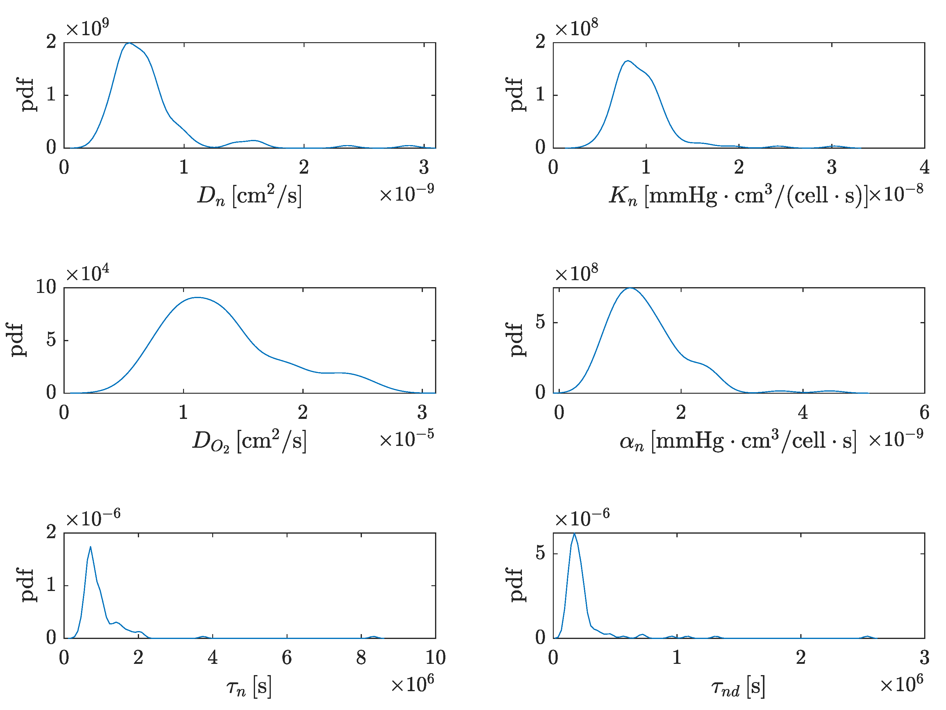
4.1.1. Marginal Distributions

First of all, we obtain the fitting of the univariate marginal distributions. Figure 2 shows the kernel estimation of the marginal distribution of the different parameters. We have chosen a Gaussian kernel for all the estimations with variable bandwidths ($w_1=7.46\times {10}^{-11}{\mathrm{cm}}^2/\mathrm{s}$, $w_2=9.52\times {10}^{-10}{\mathrm{cm}}^2/(\mathrm{mmHg}·\mathrm{s})$, $w_3=1.66\times {10}^{-6}{\mathrm{cm}}^2/\mathrm{s}$, $w_4=2.17\times {10}^{-10}\mathrm{mmHg}·{\mathrm{cm}}^3/(\mathrm{cell}·\mathrm{s})$, $w_5=9.57\times {10}^4\mathrm{s}$ and $w_6=2.74\times {10}^4\mathrm{s}$). The values are generally concentrated around the one used for the data generation, although the distributions present a variable uncertainty, related to the model complexity and its influence on the minimization procedure. For example, it is interesting to observe that all distributions present a multimodal feature, surely related to the existence of several local minima in the minimization procedure.

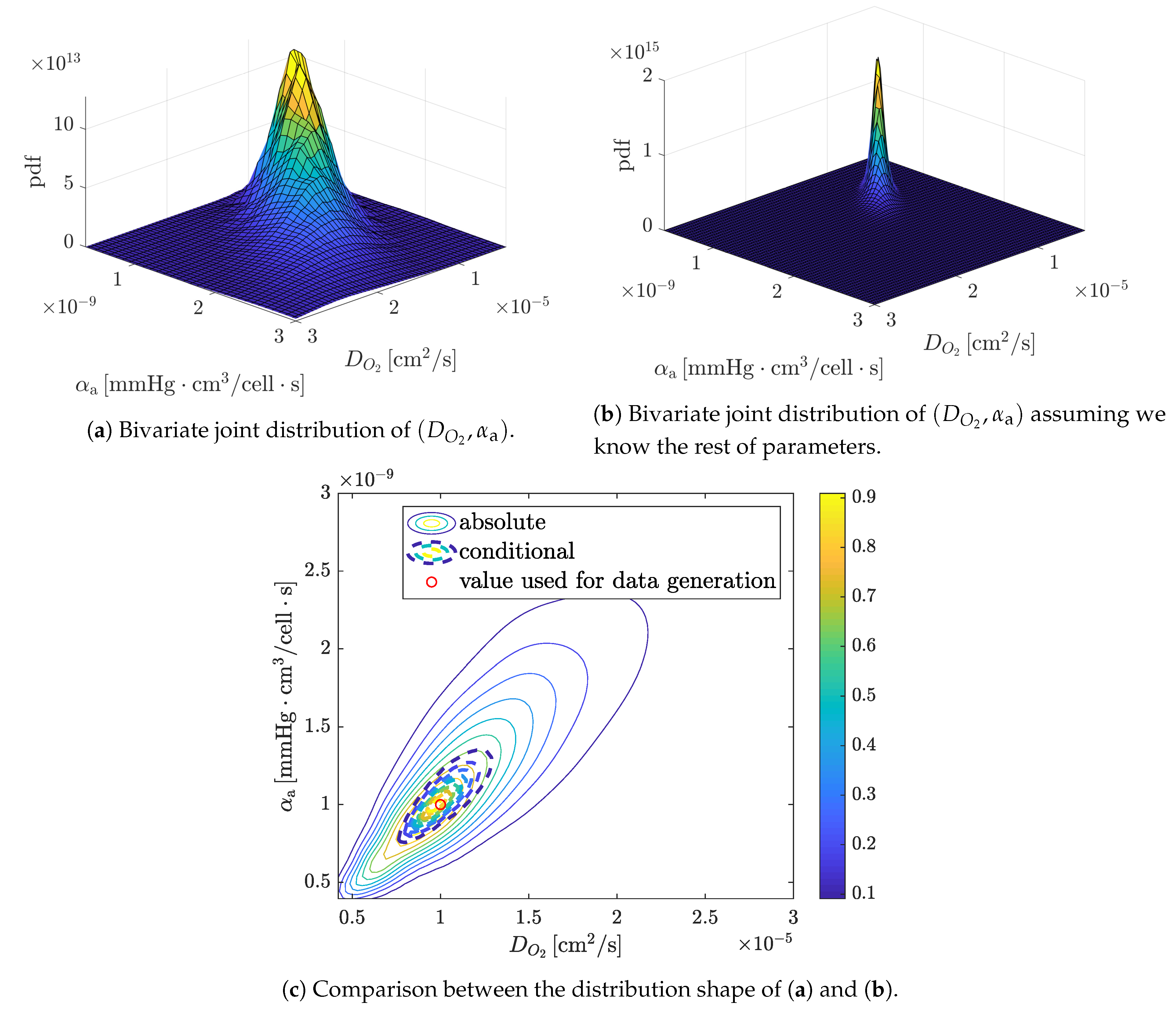
4.1.2. Parametric Copula Structure

Then, the data are transformed into uniformly distributed values using the cumulative distribution function (CDF) associated to this kernel estimation and a t-Student copula fitted by means of maximum likelihood (ML) estimation. The use of a t-Student copula is justified as it allows a different structural dependence for each of the variable pairs considered [16] and, besides, it outperforms Gaussian copula when estimating the co-occurrence of extreme events [49]. We obtain a copula with $\nu =1.8$ degrees of freedom and a Pearson correlation matrix of:

$$\mathit{P}=\left[\begin{array}{cccccc}1.00& 0.93& 0.71& 0.77& 0.70& 0.40\\ 0.93& 1.00& 0.74& 0.74& 0.77& 0.38\\ 0.71& 0.51& 1.00& 0.91& 0.61& 0.20\\ 0.77& 0.74& 0.91& 1.00& 0.54& 0.26\\ 0.70& 0.77& 0.61& 0.54& 1.00& 0.24\\ 0.40& 0.38& 0.20& 0.26& 0.24& 1.00\end{array}\right]$$

(25)

Note that the value obtained for $\nu$ is far from the Gaussian limit ($\nu \to \infty$), justifying the use of the t-Student model.

4.1.3. Complete Probabilistic Model and Bayesian a Posteriori Corrections

In order to briefly analyze the aspect of the whole model, we represent in Figure 3a the bivariate joint distribution of $(D_{O_2},{\alpha }_{\mathrm{a}})$. Knowing the whole joint distribution function allows us to make a posteriori corrections using Bayesian theory and conditional probability as explained in Section 3.2.3. If we are interested in the joint distribution of two parameters (e.g., $D_{O_2}\mathrm{and}{\alpha }_{\mathrm{a}}$), assuming that we know the rest ($D_{\mathrm{a}},K_{\mathrm{a}},{\tau }_{\mathrm{a}},{\tau }_{\mathrm{a}\mathrm{d}}$), the uncertainty of the parameter estimation obviously decreases, as can be seen in Figure 3b. In order to compare the impact of setting a posteriori the rest of the parameters, contour plots of both distributions, absolute and conditional (normalized between 0 and 1 to compare them more easily) are depicted in Figure 3c.

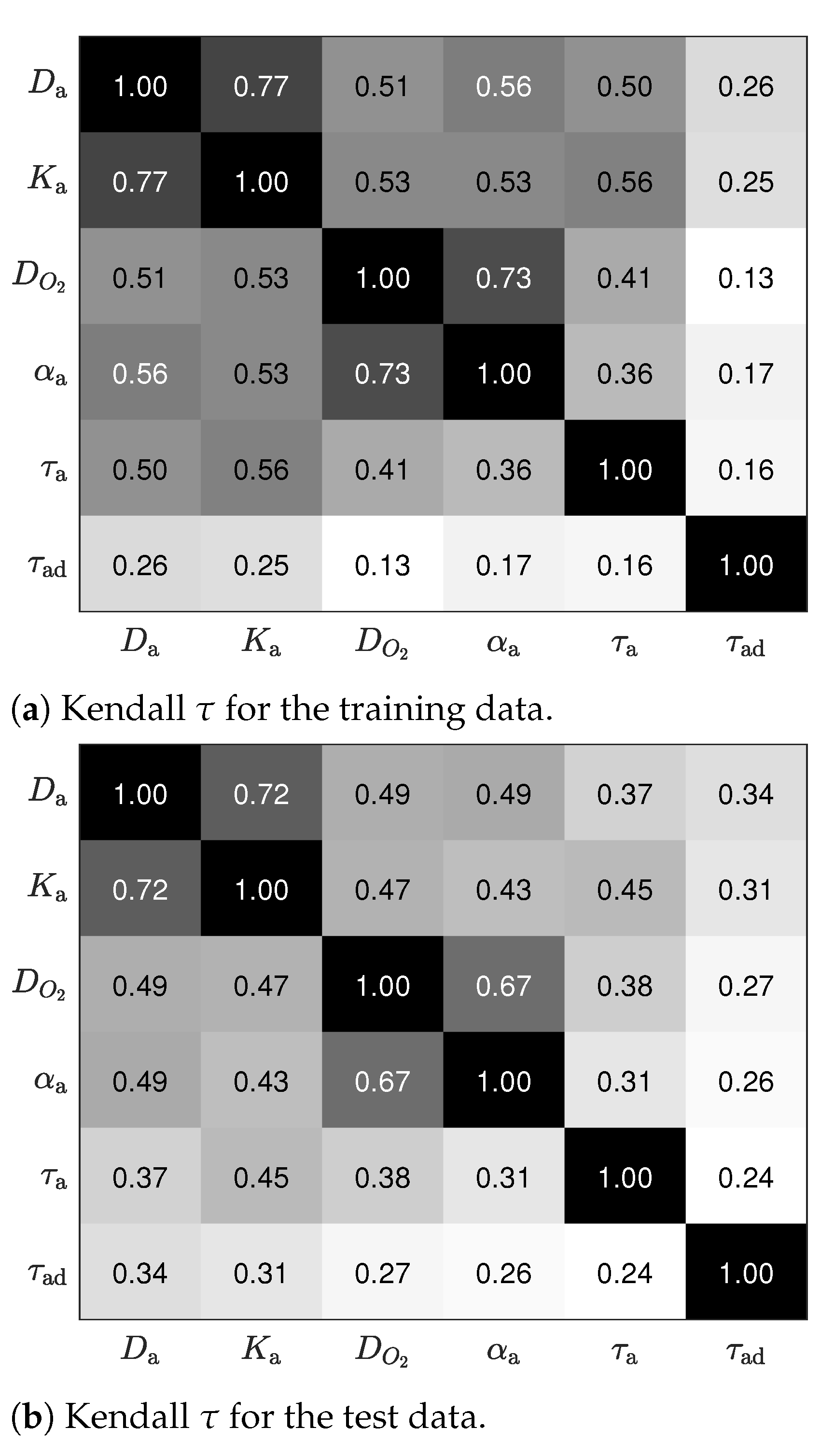
4.2. Validation of the Results Using Test Data

Over-fitting is one of the main problems in any statistical or numerical parametric fitting. In our methodology, this is avoided by using a sub-set of the data as test data for validating the models.

4.2.1. Marginal Distributions

Marginal distributions are validated as pointed out in Section 3.2. To do so, new “experimental” data are compared to the data generated from the multivariate model. It is important to note that the original data are not used, but, on the contrary, a new data-set is strictly generated from the parametric copula and marginal densities, using the same procedure described for the generation of the original data. The histogram of data, the ecdf of the test data (with $95\%$ confident interval) compared to the model data, the boxplot of both test and model data and the Q-Q plot of the test data, when compared to the model, are shown in Figure 4 for $D_{\mathrm{a}}$ as an illustrative example. The validation of the whole set of variables has been performed and good agreement was found between the model and test data except, if at all, for the extreme values, at the tail values of the distributions. In Figure 5, the ecdf of the test data for each model parameter is shown.

4.2.2. Joint Dependencies

Testing the structural dependence between parameters is not trivial. In Section 3.2, a multivariate statistical test was referenced. However, here we evaluate merely the differences in the correlation coefficients between the model-based and the test data. In Figure 6b, we represent the Kendall $\tau$ correlation index between the variables for the model and test data. We observe again a good agreement between the model values of the correlation coefficients (Figure 6a) and those obtained from the sample of the test data (Figure 6b), even though the test sample is finite, which can cause differences between the model and the statistical values.

4.3. Parameter Estimation

In Figure 7, we show p-confident HDR regions for $p=0.90$, $p=0.95$ and $p=0.99$ for the pair of variables $D_{O_2}-{\alpha }_{\mathrm{a}}$. We present the results for the absolute distribution and the conditional distribution when the rest of parameters are known. The results are compared with the classical ellipsoid estimation, which is based on the normality assumption. The differences, both in the shape and the size of the regions, are clear and are explained by the complex dependence structure between variables.

4.4. Estimation of the Output Variables

Once the multivariate distribution of the random vector $\mathsf{\Theta }$ is characterized, we know the distribution of the random vectors $\mathit{U}=\mathit{F}(\lambda ,\mathsf{\Theta })$. In Figure 8, we show the distribution of the vector $\mathit{U}$ for three experiments, which illustrates completely different behaviors corresponding to the main histopathological features of GBM. For the first one, the oxygen flow is set to $2\mathrm{mmHg}$ in the left channel and 0 in the right channel and the initial concentration of cells is $C_0=4\times {10}^6\mathrm{cell}/\mathrm{mL}$ (pseudopalisade experiment in Ref. [11]). For the second one, the oxygen flow is set to $7\mathrm{mmHg}$ in both channels and the initial concentration of cells is $C_0=40\times {10}^6\mathrm{cell}/\mathrm{mL}$ (necrotic core experiment in Ref. [11]). Finally, for the third one, the oxygen flow is set to $7\mathrm{mmHg}$ in both channels and the initial concentration of cells is $C_0=4\times {10}^6\mathrm{cell}/\mathrm{mL}$ (double pseudopalisade experiment in oxygenated conditions in Ref. [11]).

4.5. Design of Experiments

In this section, the aim is to determine the experimental configuration with the highest utility, that is, to choose both right and left oxygen flow levels and the initial cell concentration to get the maximum possible information from the new experiment. We focus here on the effect of coupling between parameters and how it affects the utility interpretation and model parameter estimation.

Two different families of simulations were carried out. In the first one, only one parameter dependence is analyzed at a time, leaving the rest fixed at the value set in Section 3.1. These figures show configurations where, if the rest of the parameters are assumed to be known, the unknown parameter will be estimated accurately. This is the case in Figure 9a,b. In the second family, two parameter dependencies are analyzed. They are considered as bivariate distributions in order to observe the effect that the parameter correlation has in characterizing these parameters, that is, how it modifies the utility values. Figure 9c, which belongs to this family, illustrates experimental configurations where the two-dimensional vector will be estimated accurately.

In Figure 9 we compare the iso-utility curves when analyzing one or two parameter dependencies for the pair of parameters related to oxygen, changes in the cell population and cell motility respectively. We assume for all figures $C_0=5\times {10}^7\mathrm{cell}/\mathrm{mL}$. In these figures we can see the most useful experiments (those configurations corresponding to the highest utility values) and those that lead to a poor adjustment of the model parameters.

This analysis may be performed for different parameter combinations, and for different degrees of knowledge. For instance,

Table 3. Different possibilities when exploring the relationship between $D_{O_2}$ and ${\alpha }_{\mathrm{a}}$ in the utility computation.

Parameters to Be Estimated	Known Parameters	Figure
$D_{O_2}$	None	-
$D_{O_2}$	$D_{\mathrm{a}}$, $K_{\mathrm{a}}$, ${\tau }_{\mathrm{a}}$, ${\tau }_{\mathrm{a}\mathrm{d}}$	-
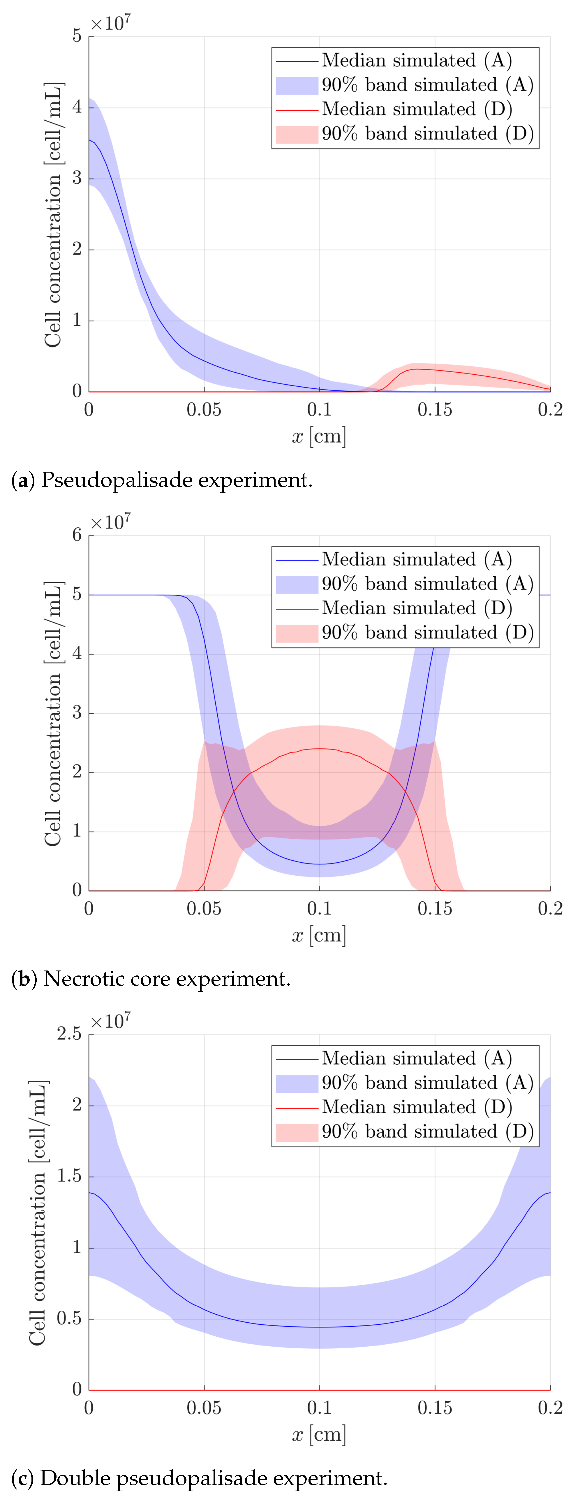
$D_{O_2}$	$D_{\mathrm{a}}$, $K_{\mathrm{a}}$, ${\tau }_{\mathrm{a}}$, ${\tau }_{\mathrm{a}\mathrm{d}}$, ${\alpha }_{\mathrm{a}}$	Figure 9a
${\alpha }_{\mathrm{a}}$	None	-
${\alpha }_{\mathrm{a}}$	$D_{\mathrm{a}}$, $K_{\mathrm{a}}$, ${\tau }_{\mathrm{a}}$, ${\tau }_{\mathrm{a}\mathrm{d}}$	-
${\alpha }_{\mathrm{a}}$	$D_{\mathrm{a}}$, $K_{\mathrm{a}}$, ${\tau }_{\mathrm{a}}$, ${\tau }_{\mathrm{a}\mathrm{d}}$, $D_{O_2}$	Figure 9b
$D_{O_2}$, ${\alpha }_{\mathrm{a}}$	None	-
$D_{O_2}$, ${\alpha }_{\mathrm{a}}$	$D_{\mathrm{a}}$, $K_{\mathrm{a}}$, ${\tau }_{\mathrm{a}}$, ${\tau }_{\mathrm{a}\mathrm{d}}$	Figure 9c

summarizes all possibilities when exploring the relationship between $D_{O_2}$ and ${\alpha }_{\mathrm{a}}$, as we are interested in the estimation of these two parameters, both individually or jointly. The cases analyzed in this paper are reported in the third column.

5. Discussion

The train-test methodology based on copulas followed in the fitting process has shown that it is possible to establish a gradation in the strength of the parameter dependencies. Figure 6a illustrates the strength of this relationship, showing that there are pairs of phenomena difficult to isolate from the experimental and/or computational points of view. For example, cell random motility and chemotaxis migration ($\tau =0.77$). Both phenomena have similar effects but in the opposite direction. Thus, it is difficult to isolate their individual effect on cell behavior if we have limited measurements available on the cell profiles. It is then only possible to evaluate, on the outcome, their combined resultant effect, that is, the average cell motility. This analysis may be done for each parameter couple, justifying the approach adopted in this work.

It is important to note that the high complexity of biological systems, resulting in coupling between pairs of variables, is moderated by the values of the rest, since the bivariate random distributions (shown for example in Figure 3a) are only a projection of the whole 6-dimensional joint distribution. Comparing Figure 3a,b, for example, we can observe the conditioning effect in location, spread, and directionality of the dependency.

Once the probabilistic model is fitted, predicting the actual value of the model parameters is easily carried out. As it is observed in Figure 7, the normality assumption for the confidence region estimation is not always a good starting hypothesis. First, it does not take into account the complexity of the relationship between the model parameters (i.e., physical phenomena) and may lead to non reliable values (meaningless physical magnitudes, such as negative oxygen diffusion). Secondly, it may mislead with respect to the uncertainty that we actually have for different significant levels. In any case, the confident region estimation using HDR and a proper probabilistic analysis are very informative about the degree of reliability of the mathematical model used for a biological explanation. These two observations become even more evident when the uncertainty of the model is reduced, as it can be seen when comparing Figure 7a,b: the chosen significant level has a major impact on the confidence region size and shape. In all the cases analyzed, this uncertainty reduction makes the confidence region to concentrate around the parameter values used in the data generation process.

Knowledge of the model parameter variation (from a probabilistic point of view) allows to predict the outcome of a given experiment. This can be used not only for model calibration and validation, but for experimental planning (deciding the appropriate material, equipment or accuracy of the measuring devices and techniques to be used). For example, in Figure 8, it may be seen that the necrotic core experiment requires less accuracy in the measurement of the cell profile in the central part of the chamber for parameter estimation, while the pseudopalisade experiment requires a measurement technique able to detect extremely low alive cell concentrations. It can also be observed that the appearance of significant alive cells at the right side of the chamber in the pseudopalisade experiment would not be explained by the model parameter variability, but rather by a model limitation.

The probabilistic knowledge of the model can be further exploited in experimental planning and design by using BED theory. In the analysis performed in this work, there are several aspects important to remark. All graphics showing the utility function are symmetric with respect to the line $O_l=O_r$. This is coherent with the symmetrical configuration of the experimental set-up (geometry and properties). The utility value should therefore not be modified by flipping the boundary conditions. Besides, it can be seen that the level curves belonging to $D_{O_2}$ and ${\alpha }_{\mathrm{a}}$ have similar shapes. This is due to the correlation between parameters, as it can be observed from the Kendall correlation coefficient $\tau$ for each pair of variables (Figure 6b). The coefficient corresponding to $D_{O_2}$ and ${\alpha }_{\mathrm{a}}$ is high and, consequently, they are strongly correlated, so the experiments needed to characterize the value of one of them are similar to the ones needed to characterize the other.

Iso-utility curves give us a picture that may be interpreted biologically and is coherent with the different phenomena occurring in the microfluidic device. However, the coupling between them makes this interpretation difficult. In this work, the utility has been computed for four different initial cell concentrations, ranging from a low concentration $C_0=1\times {10}^6\mathrm{cell}/\mathrm{mL}$ to the chip saturation concentration $C_0=C^M=5\times {10}^7\mathrm{cell}/\mathrm{mL}$. The maximum utility is always reached for the highest initial concentration ($5\times {10}^7$ cell/mL).

A summary of the analysis is presented in

Table 4. Most useful experimental configuration for each of the parameters’ evaluation.

Parameters to Be Estimated	Upper ${\mathbf{O}}_2$ Concentration [mmHg]	Lower ${\mathbf{O}}_2$ Concentration [mmHg]	Maximum Utility Value
$D_{O_2}$	7	0	$1.58$
${\alpha }_{\mathrm{a}}$	5	2	$1.53$
$(D_{O_2},{\alpha }_{\mathrm{a}})$	5	1	$2.58$
${\tau }_{\mathrm{a}}$	7	0	$0.07$
${\tau }_{\mathrm{a}\mathrm{d}}$	7	0	$1.29$
$({\tau }_{\mathrm{a}},{\tau }_{\mathrm{a}\mathrm{d}})$	7	0	$1.63$
$D_{\mathrm{a}}$	8	0	$0.51$
$K_{\mathrm{a}}$	7	1	$0.35$
$(D_{\mathrm{a}},K_{\mathrm{a}})$	8	0	$0.49$

, where the best experimental configuration is presented for each of the parameters’ calibration, together with the maximum utility value.

For the analyzed family of experiments, the most useful experiments are always the ones performed for high concentrated cell cultures. As most phenomena are related to cell concentrations, the higher the concentration, the more quantifiable the different biological mechanisms. Besides, it results clear that configurations with oxygen gradient are more useful for accurately characterizing the parameters related to oxygen ($D_{O_2}$, ${\alpha }_{\mathrm{a}}$) and cell migration ($D_{\mathrm{a}}$, $K_{\mathrm{a}}$), when the other parameters are assumed to be known. However, this gradient has to be moderate to avoid regions of total normoxia or total anoxia. When the aim is to perfectly discriminate between their effects, softer gradients are generally preferred (Figure 9c, Table 4). Finally, for high initial cell concentrations, growth and death parameters are also well characterized under gradient conditions: we need to induce localized hypoxic conditions in order to evaluate growth under saturation capacity and death.

6. Conclusions

Mathematical modeling of complex cell processes is very challenging due to its intrinsic non-linearity, highly-coupled multiphysic interactions, and the many correlated parameters which are difficult to measure or simply unknown. These parameters are most times obtained for a particular problem under specific conditions, leading in many cases to conclusions, directly derived from the modeling assumptions and therefore providing little new information. Also, they are difficult to generalize.

As a result, a proper and extensive parametric analysis is mandatory. This should include an extensive and detailed study of the values reported in the bibliography, a careful sensitivity analysis and a sufficient number of different experiments, not only for calibration but also for validation, avoiding parameter overfitting.

This analysis, although it allows the identification of the optimal set of parameters, is most times difficult to extend to other problems with reasonable accuracy and therefore with a certain validation of its actual physical character and its value range. It is also difficult to discriminate between correlated parameters associated to mechanisms that cannot be isolated in the experiments. Hence, we need additional information both to get a better discrimination between them, and to identify the optimal conditions for additional experiments to provide the maximum information possible in order to get such discrimination.

We have proved here that copulas are a simple and powerful tool to detect and improve highly-correlated multiparametric mathematical models such as those appearing in Biology, with the added value of providing key information for the optimal design of new experiments with the highest information possible for the problem in hands, thus reducing time and cost not only in our in vitro experiments but also in scarce and costly in vivo cases.

References

- Quail, D.F.; Joyce, J.A. Microenvironmental regulation of tumor progression and metastasis. Nat. Med. 2013, 19, 1423. [Google Scholar] [CrossRef] [PubMed]
- Hanahan, D.; Weinberg, R.A. Hallmarks of cancer: The next generation. Cell 2011, 144, 646–674. [Google Scholar] [CrossRef] [PubMed] [Green Version]
- Scannell, J.W.; Blanckley, A.; Boldon, H.; Warrington, B. Diagnosing the decline in pharmaceutical R & D efficiency. Nat. Rev. Drug Discov. 2012, 11, 191. [Google Scholar] [PubMed]
- Sackmann, E.K.; Fulton, A.L.; Beebe, D.J. The present and future role of microfluidics in biomedical research. Nature 2014, 507, 181. [Google Scholar] [CrossRef] [PubMed]
- Bhatia, S.N.; Ingber, D.E. Microfluidic organs-on-chips. Nat. Biotechnol. 2014, 32, 760. [Google Scholar] [CrossRef] [PubMed]
- Boussommier-Calleja, A.; Li, R.; Chen, M.B.; Wong, S.C.; Kamm, R.D. Microfluidics: A new tool for modeling cancer–immune interactions. Trends Cancer 2016, 2, 6–19. [Google Scholar] [CrossRef] [PubMed] [Green Version]
- Zervantonakis, I.K.; Hughes-Alford, S.K.; Charest, J.L.; Condeelis, J.S.; Gertler, F.B.; Kamm, R.D. Three-dimensional microfluidic model for tumor cell intravasation and endothelial barrier function. Proc. Natl. Acad. Sci. USA 2012, 109, 13515–13520. [Google Scholar] [CrossRef] [PubMed] [Green Version]
- Byrne, H.; Alarcon, T.; Owen, M.; Webb, S.; Maini, P. Modelling aspects of cancer dynamics: A review. Philos. Trans. R. Soc. Lond. A Math. Phys. Eng. Sci. 2006, 364, 1563–1578. [Google Scholar] [CrossRef] [Green Version]
- Kitano, H. Computational systems biology. Nature 2002, 420, 206. [Google Scholar] [CrossRef]
- Bearer, E.L.; Lowengrub, J.S.; Frieboes, H.B.; Chuang, Y.L.; Jin, F.; Wise, S.M.; Ferrari, M.; Agus, D.B.; Cristini, V. Multiparameter computational modeling of tumor invasion. Cancer Res. 2009, 69, 4493–4501. [Google Scholar] [CrossRef] [Green Version]
- Ayensa-Jiménez, J.; Pérez-Aliacar, M.; Randelovic, T.; Oliván, S.; Fernández, L.; Sanz-Herrera, J.A.; Ochoa, I.; Doweidar, M.H.; Doblaré, M. Mathematical formulation and parametric analysis of in vitro cell models in microfluidic devices: Application to different stages of glioblastoma evolution. Sci. Rep. 2020, 10, 1–21. [Google Scholar] [CrossRef] [PubMed]
- Brat, D.J. Glioblastoma: Biology, genetics, and behavior. In American Society of Clinical Oncology Educational Book; American Society of Clinical Oncology: Alexandria, VA, USA, 2012; pp. 102–107. [Google Scholar] [CrossRef]
- Ang, A.; Chen, J. Asymmetric correlations of equity portfolios. J. Financ. Econ. 2002, 63, 443–494. [Google Scholar] [CrossRef]
- Boubaker, H.; Sghaier, N. Portfolio optimization in the presence of dependent financial returns with long memory: A copula based approach. J. Bank. Financ. 2013, 37, 361–377. [Google Scholar] [CrossRef]
- McNeil, A.; Frey, R.; Embrechts, P. Quantitative Risk Management: Concepts, Techniques, and Tools; Princeton University Press: Princeton, NJ, USA, 2017. [Google Scholar]
- Kole, E.; Koedijk, K.; Verbeek, M. Selecting copulas for risk management. J. Bank. Financ. 2007, 31, 2405–2423. [Google Scholar] [CrossRef] [Green Version]
- Meucci, A. A new breed of copulas for risk and portfolio management. Risk 2011, 24, 122–126. [Google Scholar]
- Solari, S.; Losada, M. Non-stationary wave height climate modeling and simulation. J. Geophys. Res. Ocean. 2011, 116. [Google Scholar] [CrossRef]
- Munkhammar, J.; Widén, J. An autocorrelation-based copula model for generating realistic clear-sky index time-series. Sol. Energy 2017, 158, 9–19. [Google Scholar] [CrossRef]
- Arya, F.K.; Zhang, L. Copula-based Markov process for forecasting and analyzing risk of water quality time series. J. Hydrol. Eng. 2017, 22, 04017005. [Google Scholar] [CrossRef]
- Laux, P.; Wagner, S.; Wagner, A.; Jacobeit, J.; Bardossy, A.; Kunstmann, H. Modelling daily precipitation features in the Volta Basin of West Africa. Int. J. Climatol. A J. R. Meteorol. Soc. 2009, 29, 937–954. [Google Scholar] [CrossRef] [Green Version]
- Schoelzel, C.; Friederichs, P. Multivariate non-normally distributed random variables in climate research–introduction to the copula approach. Nonlinear Process. Geophys. 2008, 15, 761–772. [Google Scholar] [CrossRef] [Green Version]
- Laux, P.; Vogl, S.; Qiu, W.; Knoche, H.R.; Kunstmann, H. Copula-based statistical refinement of precipitation in RCM simulations over complex terrain. Hydrol. Earth Syst. Sci. 2011, 15, 2401–2419. [Google Scholar] [CrossRef] [Green Version]
- Zou, Y.; Zhang, Y. A copula-based approach to accommodate the dependence among microscopic traffic variables. Transp. Res. Part C Emerg. Technol. 2016, 70, 53–68. [Google Scholar] [CrossRef]
- Spissu, E.; Pinjari, A.R.; Pendyala, R.M.; Bhat, C.R. A copula-based joint multinomial discrete–continuous model of vehicle type choice and miles of travel. Transportation 2009, 36, 403–422. [Google Scholar] [CrossRef]
- Kilgore, R.T.; Thompson, D.B. Estimating joint flow probabilities at stream confluences by using copulas. Transp. Res. Rec. 2011, 2262, 200–206. [Google Scholar] [CrossRef]
- Bartoli, G.; Mannini, C.; Massai, T. Quasi-static combination of wind loads: A copula-based approach. J. Wind Eng. Ind. Aerodyn. 2011, 99, 672–681. [Google Scholar] [CrossRef]
- Dong, S.; Zhou, C.; Tao, S.S.; Xue, D.S. Bivariate Gumbel distribution based on Clayton Copula and its application in offshore platform design. Period. Ocean Univ. China 2011, 41, 117–120. [Google Scholar]
- Pham, H. Recent studies in software reliability engineering. In Handbook of Reliability Engineering; Springer: London, UK, 2003; pp. 285–302. [Google Scholar]
- Kim, J.M.; Jung, Y.S.; Sungur, E.A.; Han, K.H.; Park, C.; Sohn, I. A copula method for modeling directional dependence of genes. BMC Bioinform. 2008, 9, 225. [Google Scholar] [CrossRef] [Green Version]
- Kim, Y.; Jeon, H.; Othmer, H. The role of the tumor microenvironment in glioblastoma: A mathematical model. IEEE Trans. Biomed. Eng. 2017, 64, 519–527. [Google Scholar] [CrossRef] [Green Version]
- Ayuso, J.M.; Monge, R.; Martínez-González, A.; Virumbrales-Muñoz, M.; Llamazares, G.A.; Berganzo, J.; Hernández-Laín, A.; Santolaria, J.; Doblaré, M.; Hubert, C.; et al. Glioblastoma on a microfluidic chip: Generating pseudopalisades and enhancing aggressiveness through blood vessel obstruction events. Neuro-Oncology 2017, 19, 503–513. [Google Scholar] [CrossRef] [Green Version]
- Ayuso, J.M.; Virumbrales-Muñoz, M.; Lacueva, A.; Lanuza, P.M.; Checa-Chavarria, E.; Botella, P.; Fernández, E.; Doblare, M.; Allison, S.J.; Phillips, R.M.; et al. Development and characterization of a microfluidic model of the tumour microenvironment. Sci. Rep. 2016, 6, 36086. [Google Scholar] [CrossRef]
- Hatzikirou, H.; Basanta, D.; Simon, M.; Schaller, K.; Deutsch, A. ‘Go or grow’: The key to the emergence of invasion in tumour progression? Math. Med. Biol. A J. IMA 2012, 29, 49–65. [Google Scholar] [CrossRef] [PubMed]
- Stramer, B.; Mayor, R. Mechanisms and in vivo functions of contact inhibition of locomotion. Nat. Rev. Mol. Cell Biol. 2017, 18, 43. [Google Scholar] [CrossRef] [PubMed]
- Galluzzi, L.; Vitale, I.; Aaronson, S.A.; Abrams, J.M.; Adam, D.; Agostinis, P.; Alnemri, E.S.; Altucci, L.; Amelio, I.; Andrews, D.W.; et al. Molecular mechanisms of cell death: Recommendations of the Nomenclature Committee on Cell Death 2018. Cell Death Differ. 2018, 25, 486. [Google Scholar] [CrossRef] [PubMed]
- Sendoel, A.; Hengartner, M.O. Apoptotic cell death under hypoxia. Physiology 2014, 29, 168–176. [Google Scholar] [CrossRef] [PubMed] [Green Version]
- Chance, B.; Williams, G.R. The respiratory chain and oxidative phosphorylation. Adv. Enzymol. Relat. Areas Mol. Biol. 1956, 17, 65–134. [Google Scholar]
- Jaworski, P.; Durante, F.; Härdle, W.K.; Rychlik, T. Copula Theory and Its Applications: Proceedings of the Workshop Held in Warsaw, Poland, 25–26 September 2009; Springer: Berlin/Heidelberg, Germany, 2010; Volume 198. [Google Scholar]
- Sklar, M. Fonctions de repartition an dimensions et leurs marges. Publ. Inst. Statist. Univ. Paris 1959, 8, 229–231. [Google Scholar]
- Wand, M.P.; Jones, M.C. Kernel Smoothing; CRC Press: Boca Raton, FL, USA, 1994. [Google Scholar]
- Kottegoda, N.T.; Rosso, R. Applied Statistics for Civil and Environmental Engineers; Blackwell Malden: Malden, MA, USA, 2008. [Google Scholar]
- Fan, Y. Goodness-of-fit tests for a multivariate distribution by the empirical characteristic function. J. Multivar. Anal. 1997, 62, 36–63. [Google Scholar] [CrossRef] [Green Version]
- Hyndman, R.J. Computing and graphing highest density regions. Am. Stat. 1996, 50, 120–126. [Google Scholar]
- Fisher, R.A. The Design of Experiments; Oliver and Boyd: Edinburgh/London, UK, 1937. [Google Scholar]
- Chaloner, K.; Verdinelli, I. Bayesian Experimental Design: A Review. Stat. Sci. 1995, 10, 273–304. [Google Scholar] [CrossRef]
- Shannon, C.E. A mathematical theory of communication. Bell Syst. Tech. J. 1948, 27, 379–423. [Google Scholar] [CrossRef] [Green Version]
- Ahmed, N.A.; Gokhale, D. Entropy expressions and their estimators for multivariate distributions. IEEE Trans. Inf. Theory 1989, 35, 688–692. [Google Scholar] [CrossRef]
- Demarta, S.; McNeil, A.J. The t copula and related copulas. Int. Stat. Rev. 2005, 73, 111–129. [Google Scholar] [CrossRef]