Generation of 3D Turbine Blades for Automotive Organic Rankine Cycles: Mathematical and Computational Perspectives


1
Mechanical Engineering Department, Engineering College, University of Hail, Hail 81481, Saudi Arabia
2
Alasala Colleges, King Fahad Bin Abdulaziz Rd., Dammam 31483, Saudi Arabia
3
Department of Mechanical, Aerospace and Civil Engineering, Brunel University London, Centre of Advanced Powertrain and Fuels, Uxbridge UB8 3PH, UK
4
Mechanical Engineering Department, Engineering College, Suez University, Suez 43521, Egypt
*
Author to whom correspondence should be addressed.
Mathematics 2021, 9(1), 50; https://0-doi-org.brum.beds.ac.uk/10.3390/math9010050
Submission received: 17 September 2020
/
Revised: 17 October 2020
/
Accepted: 19 October 2020
/
Published: 29 December 2020
(This article belongs to the Special Issue Mathematical Modelling in Applied Sciences)
Abstract
:Organic Rankine cycle technology is gaining increasing interest as one of potent future waste heat recovery potential from internal combustion engines. The turbine is the component where power production takes place. Therefore, careful attention to the turbine design through mathematical and numerical simulations is required. As the rotor is the main component of the turbine, the generation of the 3D shape of the rotor blades and stator vanes is of great importance. Although several types of commercial software have been developed, such types are still expensive and time-consuming. In this study, detailed mathematical modelling was presented. To account for real gas properties, REFPROP software was used. Moreover, a detailed 3D CFD numerical analysis was presented to examine the nature of the flow after generating the 3D shapes of the turbine. Moreover, finite element analysis was performed using various types of materials to obtain best-fit material for the current application. As the turbine is part of a larger system (i.e., ORC system), the effects of its performance on the whole ORC system were discussed. The results showed that the flow was smooth with no recirculation at the design point except at the last part of the suction surface where strong vortices were noticed. Despite the strong vortices, the mathematical model proved to be an effective and fast tool for the generation of the 3D shapes of turbine blades and vanes. The deviations between the 1D mean-line and 3D CFD in turbine efficiency and power output were 2.28% and 5.10%, respectively.
1. Introduction
Since the late 19th century, the average temperature on Earth has risen by approximately 0.9 °C because of the increased carbon dioxide (CO2) and other man-made emissions to the atmosphere [1]. Besides the potential effects of CO2 on global climate, transportation contributes to air pollution through mono-nitrogen oxides (NOx) and particulate matter (PM) emissions [2]. Transportation also contributes to global warming through CO2 emissions which pose serious threats to public health. Among fuel-based applications, transportation burns most of the world’s fuel, accounting for more than 28% of the total fuel consumption in the United States in 2018 [3] and more than 50% in the United Kingdom [4]. In addition, fuel prices have continually increased, from 1.191$/gallon in 1990 to 2.578$/gallon in the US [5]. Additionally, with the improvement of people’s living standards, fuel consumption by the transportation sector will increase significantly [6]. These concerns necessitate the development of more efficient combustion engines to reduce fuel consumption and CO2 emissions. In this regard, waste heat recovery (WHR) technology is one of the promising technologies in recovering the wasted fuel energy.
Lately, organic Rankine cycle (ORC) systems have gained lots of attention for recovering waste heat from low to medium temperature heat sources [7]. Compared to other WHR technologies, ORC systems present high thermal efficiency under a wide range of operating conditions [8], relatively low cost and minor increase of pumping losses [9]. The implementation of ORC systems in internal combustion engines (ICEs) is found to significantly improve fuel consumption by up to 5% [9], while another study reported that engine exhaust emissions (especially NOx) drop as engine load is minimized [10]. More recent studies show the high potential of ORC systems as WHR technologies in ICEs. Karvountzis-Kontakiotis et al. [11] studied the effects of variable geometry turbine performance on the thermal cycle performance. Compared to fixed geometry turbines, the thermal efficiency of the cycle with variable geometry turbine variable was 32.2% better. Zhang et al. [12] developed an experimental system to recover wasted heat in the exhaust gas of a heavy-duty diesel engine. The results indicated that the maximum power output, ORC efficiency and overall system efficiency were respectively 10.38 kW, 6.48% and 43.8%. Guillaume et al. [13] used exhaust gases of a truck diesel engine as the heat source for their ORC system. They used a radial inflow turbine as the expansion machine and two working fluids: R245fa and R1233zd. The maximum electric power and turbine efficiency were 2.8 kW (using R245fa) and 32% (using R1233zd), respectively. Alshammari et al. [14,15] explored the potential of integrating an ORC as WHR technology in heavy-duty diesel engines. The authors used an intermediate thermal oil loop to ensure steady-state operation. Although operated at off-design conditions, electrical power of 9 kW was generated. Lion et al. [16] investigated different engine-ORC architectures using a large two-stroke marine diesel engine. The results proved the ability of ORC to reduce the engine fuel consumption by 5.4% at full load. Imran et al. [17] developed a multi-objective optimization model of an organic Rankine cycle system using the exhaust gas of a heavy-duty diesel engine at 40% load. At the design point, a net power output of 10.94 kW was obtained. Mat Nawi et al. [18] extracted the wasted heat in a 996 kW marine engine with an exhaust temperature of 573.15 K using an ORC system. The obtained system efficiency and net power were 2.28% and 5.10 kW. Ezoji and Ajarostaghi [19] performed thermodynamic-computational fluid dynamics (CFD) analysis to recover wasted heat from the coolant system (water jacket) in a six-cylinder homogeneous charge compression ignition (HCCI). Results indicate that the improvement in thermal performance of the hybrid system in the HCCI engine can be as high as 27.94%. Yue at al. [20] proposed a mathematical model for vehicle energy supply system using ORC system and various turbine inlet temperatures. The maximum thermal efficiency of 37.5% was obtained using cyclo-pentane as the working fluid. The results showed also that the maximal gasoline oil saving rate at 9.73 kg/h, and the minimal payback period at 769 h were achieved. Liao et al. [21] investigated the potential of recovering waste heat from a coal-fired plant. The results showed a maximum thermal efficiency of 16.37%. Liu et al. [22] developed a new system for harvesting wasted heat aiming at reducing fuel consumption and exhaust emissions of a 14-cylinder marine engine, by combining steam and organic Rankine cycles. The results showed that the thermal efficiency of the engine could be improved by 4.42% and the fuel consumption could be reduced by 9322 tons per year. Le Brun et al. [23] analyzed the feasibility and prospects of small-scale commercial combined ICE + ORC CHP systems. They concluded that the installation of 40 kWe ORC system e alongside a 400-kWe ICE-CHP system can lead to an increase in overall efficiency from 51.7% to 54.0%, and a reduction of 2% in carbon emissions. Ochoa et al. [24] studied the feasibility of integrating ORCs in internal combustion engines using advanced exergo-environmental modelling. The results showed that BSFC and CO2 emissions could be improved significantly using ORC systems.
Among the components of the ORC system, the expansion machine is the most crucial because of its significant effects on the performance, size and cost of the overall cycle [25]. Radial inflow turbines appear as the main tool to improve the energy efficiency of automotive powertrain systems [26]. Although mean-line modelling consumes up to 50% of the total engineering time during radial turbine design [27,28], some conditions require a good geometrical representation [29]. Mean-line modelling is yet incapable of capturing the flow behaviour, such as flow separation and shock waves. Thus, 3D simulations are essential [30]. Within the turbine, the rotor is the key component to produce work. Ahead of starting the 3D simulations, the 3D shape of the turbine blades and vanes should be generated. Most of the studies in the literature use commercial software for this task. However, such types of software are expensive and time-consuming. This makes it imperative to develop fast and accurate mathematical modelling for blade generation. As small-scale radial inflow turbines are characterized with small mass flow rates, the turbine usually adopts radial blades at the inlet (zero-degree blade angle). Radial inlet blades are beneficial to avoid bending stresses. To increase the turbine work (enthalpy drop within the rotor), the tangential velocity at the rotor inlet should be increased as explained un the previous study [31]. Using backswept (non-radial) blades results in positive relative angle and consequently, larger enthalpy drop. However, utilizing backswept blades results in higher bending stresses at the rotor leading edge and failure is likely to occur, leading to catastrophic consequences both physically and economically. Therefore, it is very essential to ensure that the turbine rotor can withstand the operating conditions of the flow and have adequate life in service. Therefore, structural evaluation of the turbine stage using FEA, which is widely applied in the analysis of engineering problems [32], is essential. Colonna et al. [33] developed an in-house Euler solver to perform complete CFD simulations for supersonic turbines. They mainly focused on the effects of different equations of state (EoS) for real gases. The results showed a significant deviation when an ideal gas EoS was applied, while the Span–Wagner and Peng–Robinson–Stryjek–Vera equations were very similar. Harinck et al. [34] performed a complete steady-state simulation for their supersonic radial inflow turbine using ANSYS CFX. The property tables were generated using REFPROP [35]. Their results showed that the improved stator model was able to deliver the required tangential velocity components with a Mach number value as high as 2.85. Sauret and Gu [36] presented 3D CFD simulations of ORC radial inflow turbines using commercial software to validate the mean-line model. The results showed good agreement between the mean-line and numerical results. The results also showed the significant effects of the turbine off-design conditions on the ORC system. Uusitalo et al. [37] simulated a high supersonic small-scale ORC turbine stator where a real gas model was implemented in a CFD solver using both the 𝑘 − 𝜀 and 𝑘 − 𝜔 𝑆𝑇𝑇 turbulence models. The results showed that Mach number at the stator exit was 2.27 for 𝑘 − 𝜀 solver and 2.31 for 𝑘 − 𝜔 𝑆𝑇𝑇. Recently, White [38] performed a full CFD analysis using ANSYS CFX as a validation for his mean-line model of the ORC radial turbine. The agreement between the mean-line and CFD was very good with a deviation of 0.3% in the total to static efficiency. He also validated his model with the CFD by comparing the stagnation and static thermodynamic properties at the inlet and exit of the turbine rotor. The results were very accurate with a maximum deviation of 6.3% in the static pressure at rotor inlet. Similarly, Verma et al. [39] validated his 1D model with a complete CFD simulation using ANSYS CFX, and the deviation between the mean-line and CFD simulation in the turbine efficiency was 0.17%. Their CFD results showed a choking condition at the design point with Mach number of 1.55. Nithesh and Chatterjee [40] presented a study that combines 1-D design and 3D CFD. The numerical CFD analyses were in good agreement with 1-D model. Song et al. [41] studied the performance of radial outflow turbines at off-design conditions using 1D and CFD analyses. Their 1D results correlated well with the CFD results. Daabo et al. [42] presented two design models for axial and radial turbines to be used in solar powered Brayton cycles. Their CFD analyses were validated against experimental work and then used to validate the mean-line models. Dong et al. [43] explored the sensitivity of turbine design to some design parameters such as stator velocity coefficient. The proposed model was followed by a detailed CFD study in which a good agreement was obtained. Sun et al. [44] investigated the effects of non-equilibrium condensation flow on the performance of radial inflow turbines using CFD studies. Wang et al. [45] studied the effects of different zeotropic mixtures on the design of radial inflow turbines. There 1D results were compared with extensive CFD analyses and presented a maximum deviation of 5.02% in turbine power. Recently, Schuster et al. [46] presented an optimization model for ORC radial inflow turbines supported by CFD analyses. Their results showed sufficient agreement between 1D and CFD results. The brief review shows that CFD analysis allows the calculation of the flow field considering the viscous effects which are usually neglected in 1D model. Moreover, CFD can be applied as a reference of validation of mean-line models. Al Jubori et al. [47] developed a 1D mean-line model for designing a single stage radial turbine accompanied with CFD and experimental investigations. The results showed a tight race between the mean-line model and CFD. Flores et al. proposed a unidimensional design approach for a 10 kW radial inflow turbine. Both theoretical and numerical, proved to be in a good approximation.
In turbomachines, the rotor is the key component to produce work [48]. As small-scale radial inflow turbines are characterized with small mass flow rates, the turbine usually adopts radial blades at the inlet (zero-degree blade angle). Radial inlet blades are beneficial to avoid bending stresses. To increase the turbine work (enthalpy drop within the rotor), the tangential velocity at the rotor inlet should be increased according to the Euler equation as explained un the previous study [31]. Using backswept (non-radial) blades result in a positive relative angle which results in larger tangential velocity and hence, larger enthalpy drop. However, utilizing backswept blades results in higher bending stresses at the rotor leading edge. Failure is likely to occur when stresses are greater than the yield stress of the material of the rotor which may lead to catastrophic consequences both physically and economically [49]. The main challenge in the operation of turbine blades is the harsh operating environment (high temperature, high pressure and high rotational speed) in which thermal and structural stresses can result which further leads to creep and fatigue phenomenon and finally failure of the blades. Therefore, it is very essential to ensure that the turbine rotor can withstand the operating conditions of the flow and have adequate life in service. Therefore, structural evaluation of the turbine stage using FEA, which is widely applied in the analysis of engineering problems [50], is essential.
Research on bending stresses in ORC turbines is an area in which little available literature exists. However, enough studies were conducted aiming at analyzing bending stresses on air and steam turbines. Chen and Xie [51] created a finite element model of a low-pressure turbine blade to investigate the elastic-plastic conditions considering centrifugal load and aerodynamic load. Similarly, Fu [52] created a three-dimensional finite element model of the turbine blade to analyze the stress distribution of the turbine blade based on the thermo-elastic-plastic finite element under the conditions of centrifugal load and temperature load. Odabaee et al. [53] presented an FE analysis of a high-pressure ratio single stage radial-inflow turbine using ANSYS. The results showed a good agreement between the numerical and experimental data. Gad-el-Hak [54] presented a coupled CFD-FEA study with air as the working fluid and compared the results with experimental data. Similarly, Xie et al. [55] investigated the flow environment and blade thermal stresses using ANSYS with air as the working fluid. The authors considered both the thermal load and the centrifugal load. Banaszkiewicz [56] presented a methodology for analyzing both axial and radial stresses in steam turbine rotors and compared the proposed model with different methods available in the literature. Wang et al. [57] studied the effects of active thermal management on failure risk of disks and explores possible means for risk control. They concluded that the probability of disk failure increases with increasing the load cycle. They also concluded that the disk hub is the riskiest part and strongly influences the disk safety.
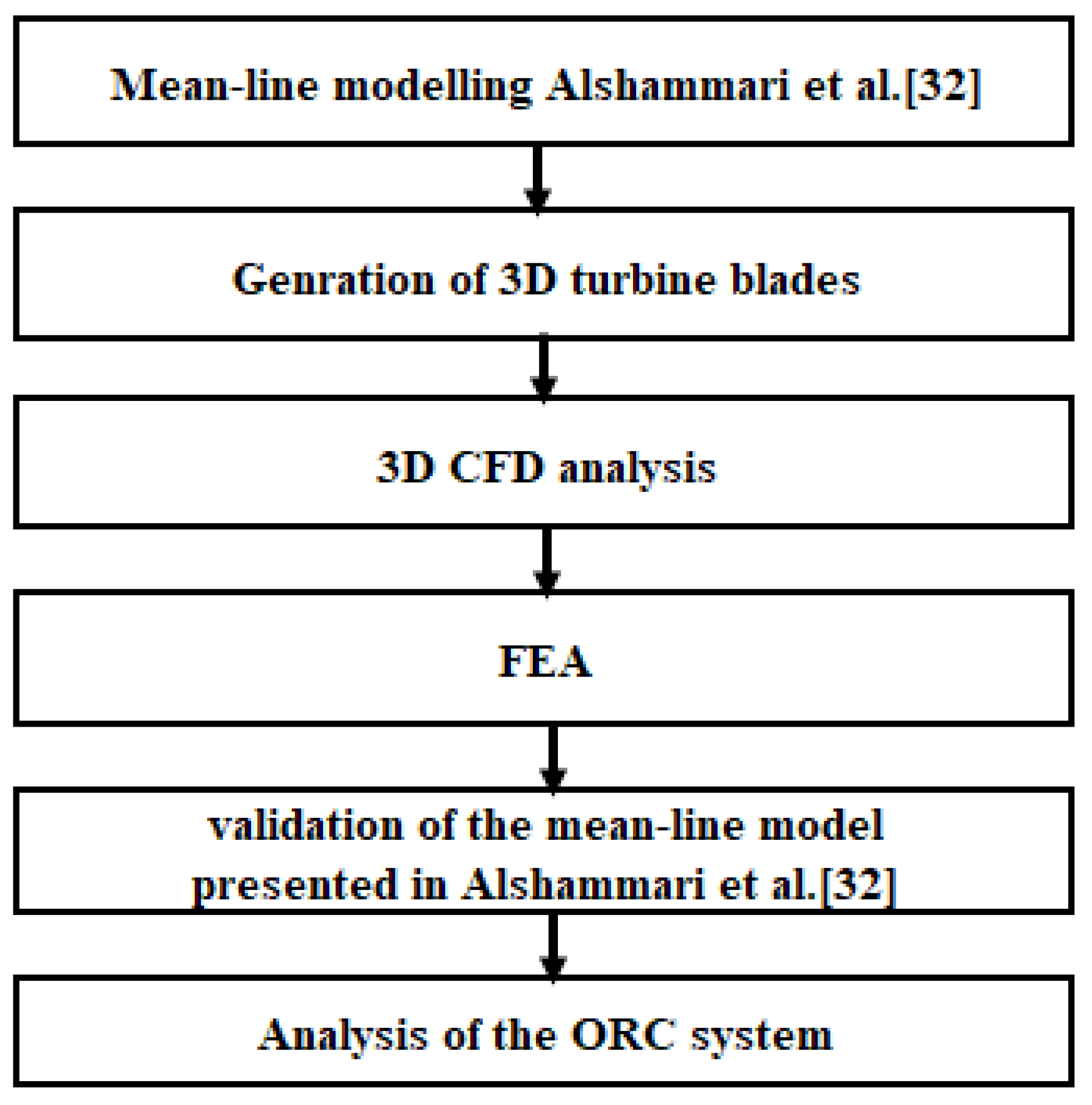
The brief literature review in the above paragraphs indicates the importance of developing a fast and accurate mathematical modelling of blade generation. Moreover, CFD and FE analyses are crucial steps for checking the turbine feasibility before sending the turbine for manufacturing and hence saving money. Moreover, ORC radial inflow turbines usually operate with the high-pressure ratio which necessities a careful examination of the flow environment, especially at the stator exit (due to the high Mach numbers at this region). In addition, ORC systems operate with high dense real fluids (organic fluids). Therefore, proper modelling of the fluid properties should be considered. Very importantly, it can be noticed that the non-radial (backswept) blade in radial turbines is an area in which little available literature exists. Therefore, the proper mathematical modelling of backswept blades is presented. In addition, the thermodynamic parameters of the exhaust gas, such as mass flow rate and temperature can vary widely with time in heat sources such as ICEs. This variance causes heat sources to become unstable and uncontrollable. Therefore, the performance behaviour of the 3D shaped turbine when running at off-design rotational speeds and pressure ratios should be accurately predicted. In addition, the radial inflow turbine is part of a larger system which the ORC in the current study. Therefore, it is of great importance to analyze the performance of the ORC system under various operating conditions of the turbine. Moreover, the brief literature review also indicates the success of CFD discipline in validating mean-line models. This study aims at filling these gaps by providing a complete 3D-shape generation and CFD-FE analyses at design and off-design conditions. Figure 1 presents a flowchart of the current study.
2. Organic Rankine Cycle and Radial Inflow Turbine
Typical ORC consists of four main components, namely: evaporator, turbine, condenser and pump, Figure 2. The working fluid is vaporized in the evaporator (7 to 1) and then expanded in the turbine (1 to 5) that drives a generator to produce electricity. Finally, the working fluid is condensed at constant pressure (5 to 6) and pumped again (6 to 7) to the evaporator. Points 1 to 5 represent the turbine stage as shown in Figure 3.
The detailed description of the ORC system and internal combustion engine can be found in the previous studies of the authors [14,15]. Three different radial inflow turbines were designed in the previous study [31], a separate turbine for each engine operating point. In this study, the operating conditions of the exhaust gas at P3 is selected as the heat source of the current study. In addition, the geometry of the radial inflow turbine of P3 is considered in the current simulation since P3 is considered as the optimum engine point. The detailed geometry of the P3 turbine can be seen in [31]. Table 1 presents the input conditions for the mean-line model, which are used as the input conditions for the current CFD study. Table 2 summarizes the basic equations in ORC and radial inflow turbine applied in the current study.
3. Generation of 3D Model
This section presents the construction of the 3D model of the turbine stage, namely, stator and rotor. The volute is excluded since the losses are extremely small compared to the losses in the stator and rotor. Although the 3D generation of turbine blades and vanes have extensively explained in the literature such as in Aungier [27]. However, these equations are related to ideal gas equations of state. In the current study, real gas properties of the fluid have been accounted for using REFPROP [35].
3.1. Stator Model
The inlet and exit vane angles are 76.335° and 66.75°, respectively, as obtained from the turbine mean-line model [31]. The distribution of thickness is performed according to the procedure proposed by Aungier [27]. The thickness distribution is performed on a parabolic-arc camber-line as outlined in Aungier [27]. The governing equation for a parabolic-arc camber-line is shown in Equation (7). The coordinate (x,y) is shown in Figure 4. and are the location and value of maximum camber along the chord, respectively. and are camber-line angles at inlet and exit, respectively.
The stator geometrical parameters can then be obtained based on the value of . The required parameters are chord length , maximum camber and its location . The leading and trailing edge blade angles can be obtained using Equations (8) and (9). The angle of the blade comber-line is then the sum of the two-blade angles.
Aungier [27] proposed several equations to calculate the blade thickness at any location along the camber-line as shown in Equations (10)–(14).
3.2. Rotor Model
For the construction of the rotor, three geometrical aspects were constructed to generate the full rotor blade. These aspects are meridional profiles, blade angle distribution and thickness distribution.
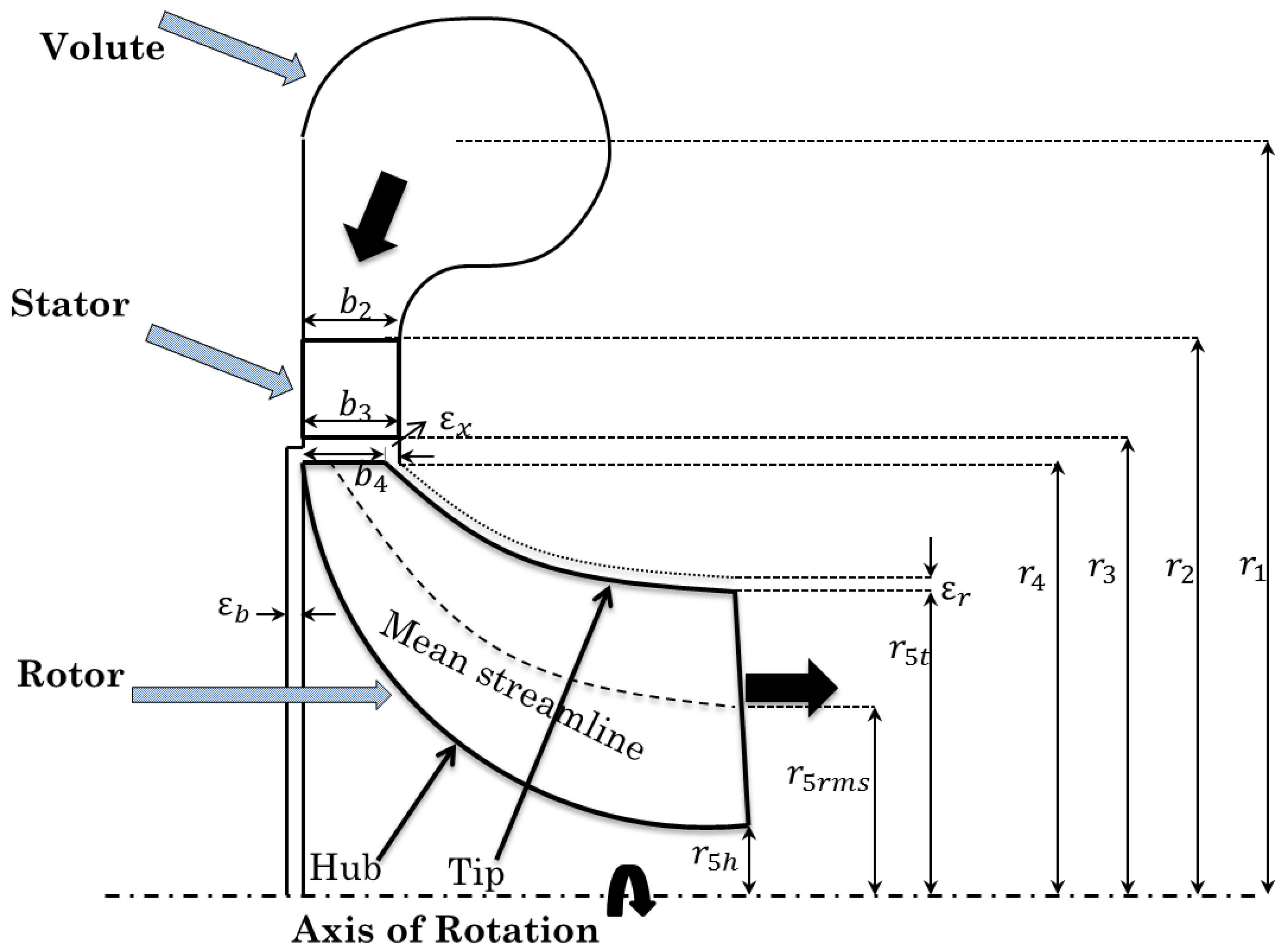
The 2D rotor meridional profiles (end-wall contours) are defined by applying the methodology presented in Aungier [27]. In this study, a quarter ellipse is applied to define the three meridional profiles, namely, hub, mid and shroud, as shown in Figure 7. As explained in the previous study [31], , , and are the inlet blade height, inlet blade radius and axial length, respectively.
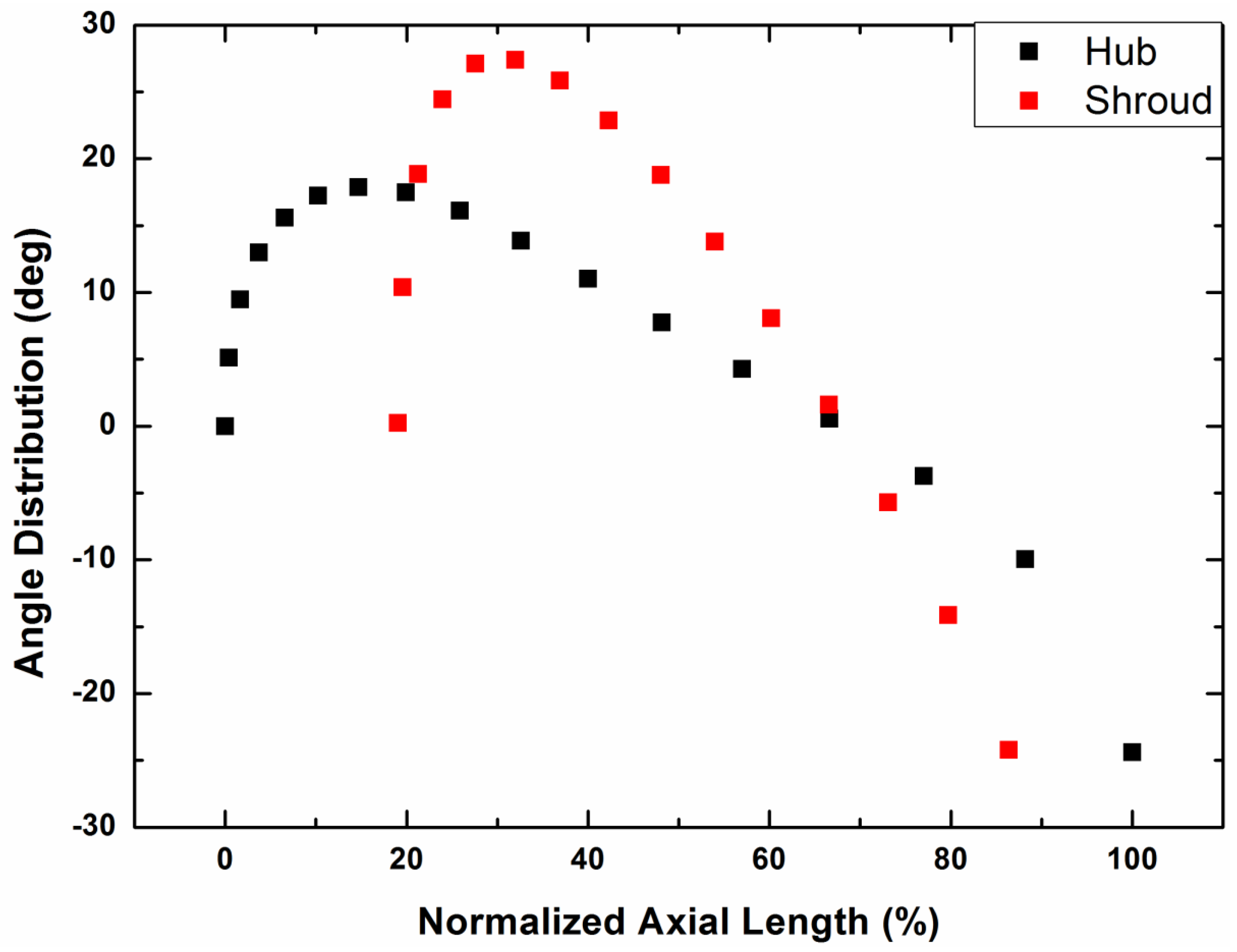
In the current study, the blade is not radially fibred. The blade distribution of blade angles is determined by the numerical integration of Equations (15) and (16), where 𝑚 is the meridional distance along the 𝑍 − 𝑅 contour, Figure 7. The coefficients to are summarized in Table 3. Equation (15) is the blade camber-line along the shroud contour, whereas Equation (16) is the camber-line along the hub contour. The distribution of the blade angle is shown in Figure 8.
Blade thickness is distributed in three regions, namely, leading-edge, meridional profile, and trailing edge. As will be shown later, blade root is the location where stress is the highest. Therefore, this region must be the thickest to improve the weight distribution of the blade. To obtain thick root, the blade is tapered from hub to tip. Thicknesses at inlet and exit of the leading edge and trailing edge, Figure 9, are calculated using Equations (17)–(20) [27,58]. and are the tip and hub exit thicknesses and obtained from the mean-line model [31]. In the current study, the blade thickness at the hub ( is obtained using Equation (20) to keep thicker root. Figure 9 also presents the developed 3D rotor blade.
4. Computational Fluid Dynamics (CFD)
Before sending the turbine out for manufacturing, a complete CFD study of the full turbine stage is accomplished using ANSYS CFX [59]. In this section, the setup of the turbulence model, physical domain, boundary conditions and the organic fluid (NOVEC 649) are presented. A grid-independent study is also performed to ensure that the results are independent of the number of nodes. Figure 10 presents the flowchart of the adopted numerical analysis and Figure 11 presents a 3D view of a radial turbine stage and boundary conditions.
4.1. Grid Generation of the Fluid Model
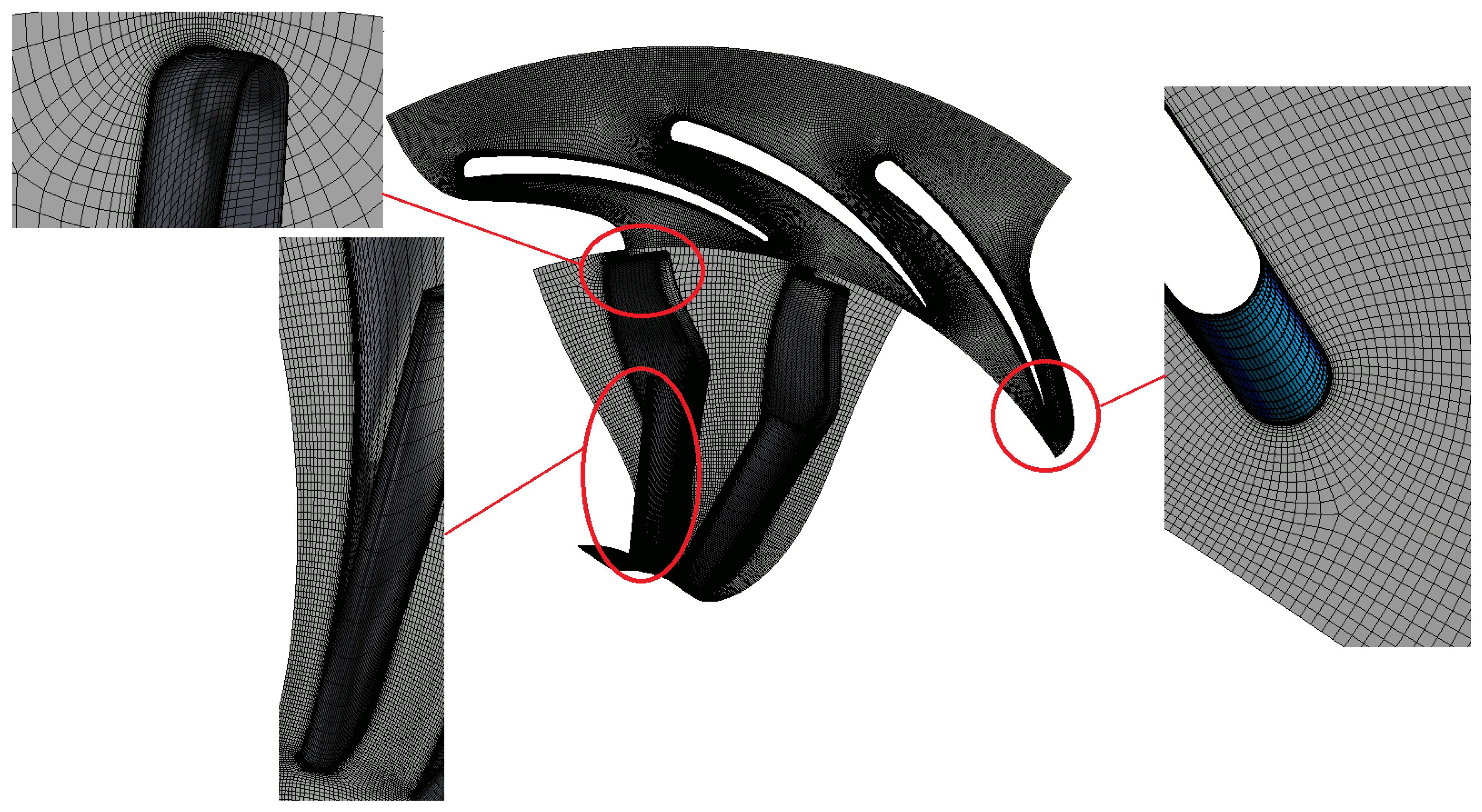
In the current study, the solid parts are imported to ANSYS TurboGrid to generate the appropriate meshes, as shown in Figure 12. An automatic topology (ATM Optimised) is selected so ANSYS TurboGrid could select the suitable topology for the blade passage. If the mesh quality at a certain region, such as the rotor leading edge, is poor, then the control points can be adjusted by the user to solve the problem. Figure 13 presents the sensitivity analysis of the element number of the passage to the turbine isentropic efficiency and the static exit temperature at the rotor exit.
4.2. Turbulence Model, Physical Domain, Boundary Conditions, and Governing Equations
During the past two decades, two main turbulence models have been developed: model, which is based on the turbulence dissipation rate , and model, which is based on the specific dissipation rate. Fajardo [60] indicated that is more accurate than in computing the near-wall layers. However, converges faster and is robust with real gas applications [36]. Menter [61] developed less complex and less computationally expensive model called shear stress transport () model. The SST model applies the model to capture the near-wall region accurately and switches to the model in the free-stream to avoid the sensitivity of to the effects of free-stream turbulence. Menter’s predicted results using the model are in good agreement with the experimental data. Therefore, is applied in the current analysis for both the design point and off-design analyses.
To reduce computational time, a single flow passage for the rotor and stator is simulated and rotational periodicity is applied by setting an appropriate pitch ratio at the interface between the stator and rotor. Different meshing is required because of the different components considered in the simulation. Therefore, the position of the grid nodes in one domain may not match those in the other domains. The general grid interface is applied to avoid such non-matching interface. Domain interfaces are required because a change in reference frame between stationary (stator) and rotating (rotor) domains occurs. ANSYS CFX has two main interfaces, namely, mixing plane and frozen rotor. The main difference between the two interfaces is that the mixing plane applies the average qualities on the interface for upstream and downstream components; therefore, it is applied in the current study. Figure 14 shows the modelled components with the corresponding fluid domains.
Navier–Stokes equations that are discretized by a finite volume approach are integrated into the current study. These equations are applied to solve for velocity, pressure and temperature associated with a moving fluid. Navier–Stokes equations describe the conservation of mass, momentum and energy, as shown in Equations (21)–(23), respectively. The Reynolds’s average Navier–Stokes (RANS) equations are also used to account for the turbulence in the flow. These equations are solved to obtain the time-averaged properties of the flow without the need for resolution of the turbulent fluctuations.
5. Finite Element Analysis (FEA)
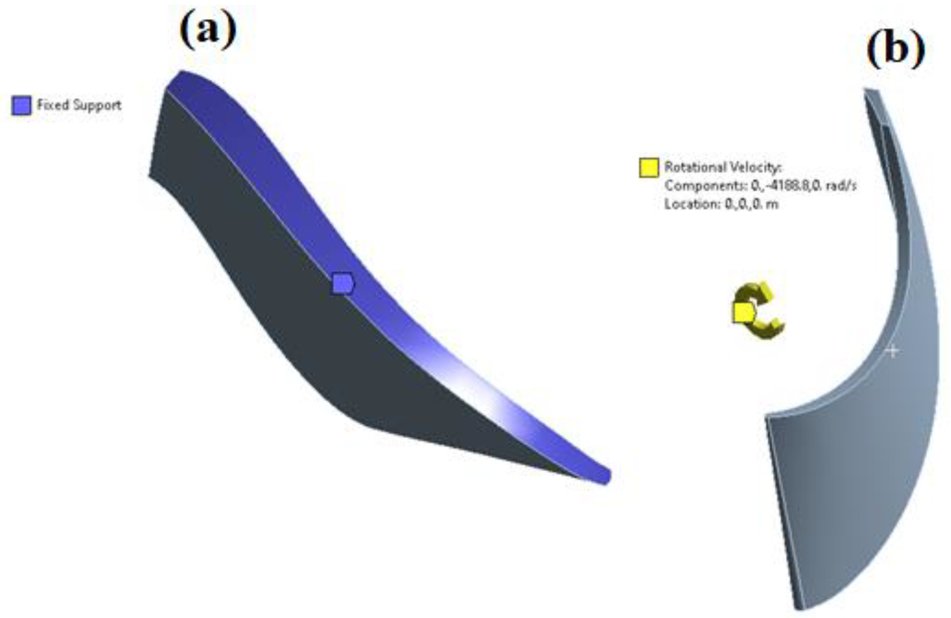
Rotors in radial inflow turbines experience aerodynamic and mechanical loads. Therefore, it is essential to investigate the mechanical integrity of such components. In addition, rotor blades in conventional radial turbines are usually radially fibered (zero inlet blade angle) to minimize bending stresses. However, since backswept blades are used in the current study, the centrifugal stresses at the leading edge must be analyzed and checked carefully. The purpose of the current analysis is to identify the limits of blade tip deformation and total von Mises stresses using ANSYS Static Structure. The resulted maximum stress and displacement should not exceed the material tensile strength and the running tip clearance (0.6 mm [31]). The running tip clearance is the clearance between the rotor and the casing. Figure 15 shows the specified fixed support and direction of rotation.
5.1. Material Selection
Various types of materials are investigated. Fullcure 720 which is a multipurpose Polymer is considered as a cost-effective and efficient way for turbine manufacturing [62]. In other studies [63,64], rotor blades are made of the aluminium alloy due to its light weight, ease of machining, strength-to-weight ratio and corrosion resistance. In Kaczmarczyk et al. [65], rotor blades were made of stainless steel to provide adequate heat compensation and minimize the propagation of vibrations of the machine to the entire installation. Moreover, rotors made of Titanium alloy are used in some studies such as [66,67] to provide high mechanical resilience. Table 4 presents the properties of considered types of materials.
5.2. Mesh Generation and Sensitivity Analyses
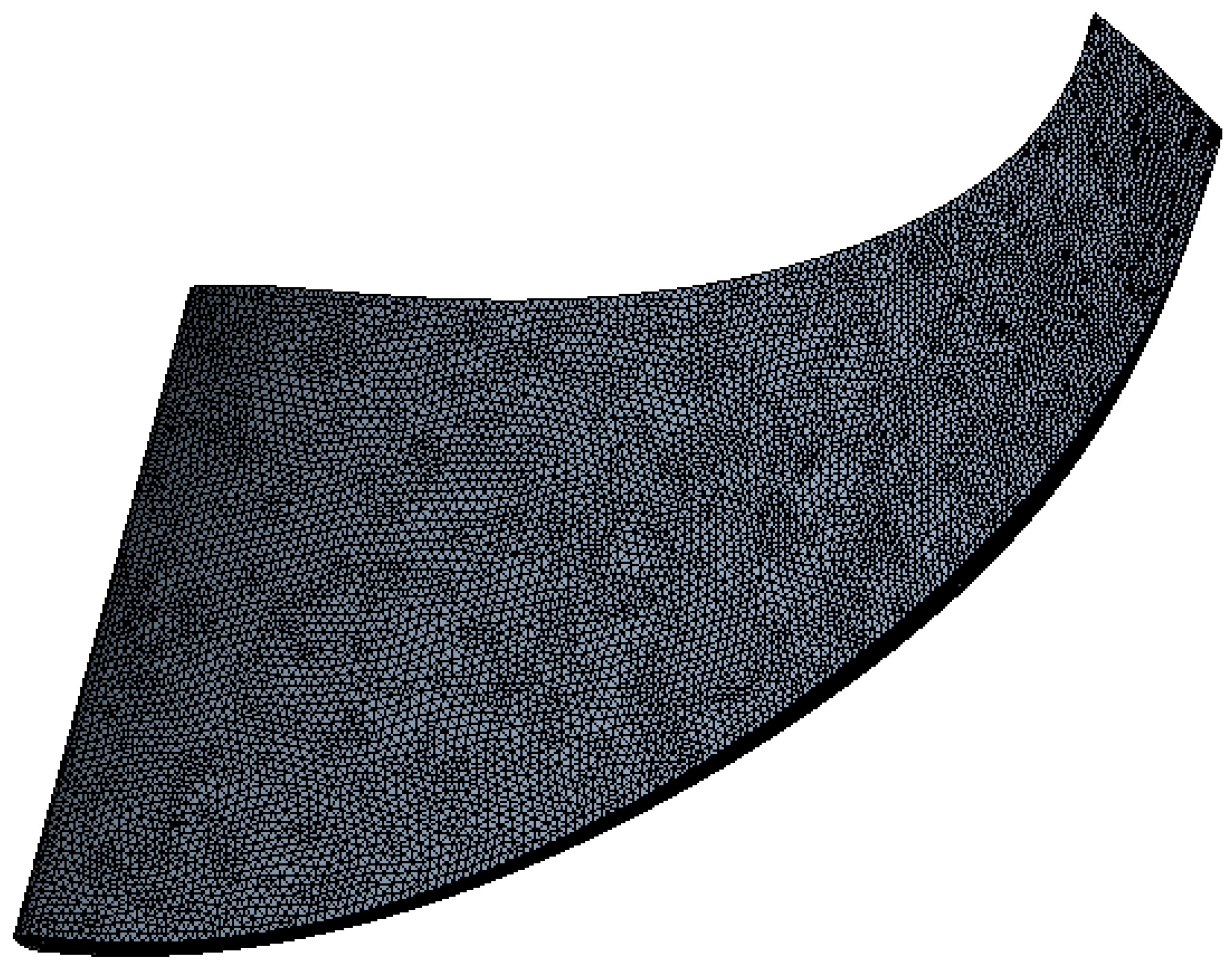
Like the CFD study, the independency study for FEA is carried out using different element sizes as shown in Table 5. Several meshes are generated with different node numbers. The deviation between two executive operations decreases till reaches 0.33% in von Mises stress and 0.002% in total deformation between operation 8 and operation 9. Therefore, the mesh in operation 8 is selected as the grid independence values. The mesh of the turbine rotor is generated with mapped face/tetrahedrons mesh type as shown in Figure 16.
6. Results and Discussions
6.1. Computational Fluid Dynamics (CFD) Results
6.1.1. Validation of the Numerical Analysis
Although CFD is a powerful and robust simulation tool, it still needs to be verified experimentally. The turbine model has already been manufactured and tested as shown in the previous studies of the authors [14,15]. Unfortunately, the test has been run at highly off-design conditions due to the technical issue of the engine dynamometer. Therefore, the test results cannot be directly used to verify the proposed mean-line model. However, the test results can be applied to validate the numerical analysis. Therefore, the test results of the study [14] are used to validate the CFD results in the current study.
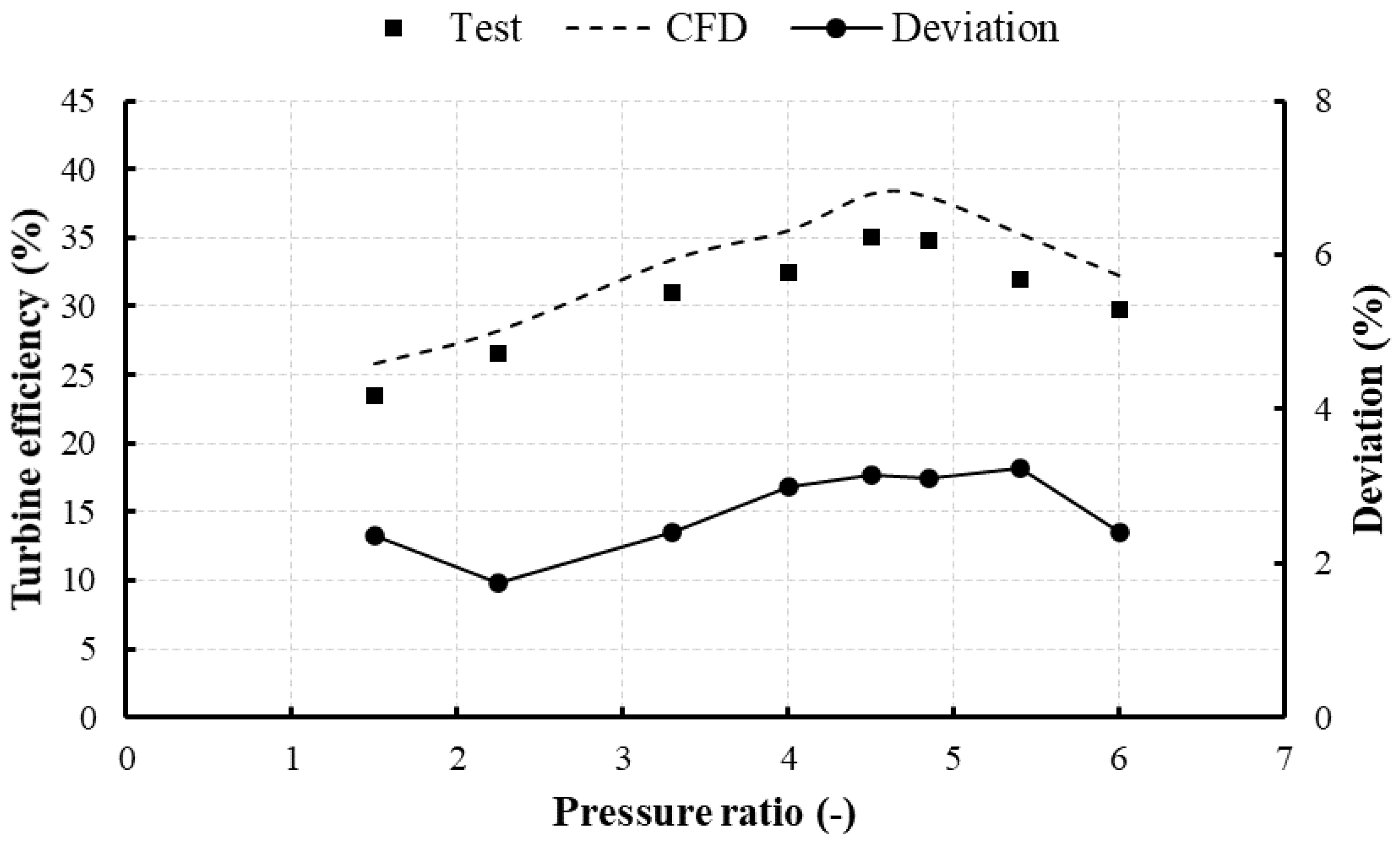
Figure 17 shows a comparison between the CFD and test results at 20,000 rpm for different pressure ratios. As seen in the figure, the CFD numerical results show very good agreement with the test results. A maximum deviation of 3.23% is noticed at a pressure ratio of 5.4, while the average deviation is 2.67%. Therefore, the current CFD model can be applied more confidently as a validation model for the proposed mean-line model.
6.1.2. Results at Design Point
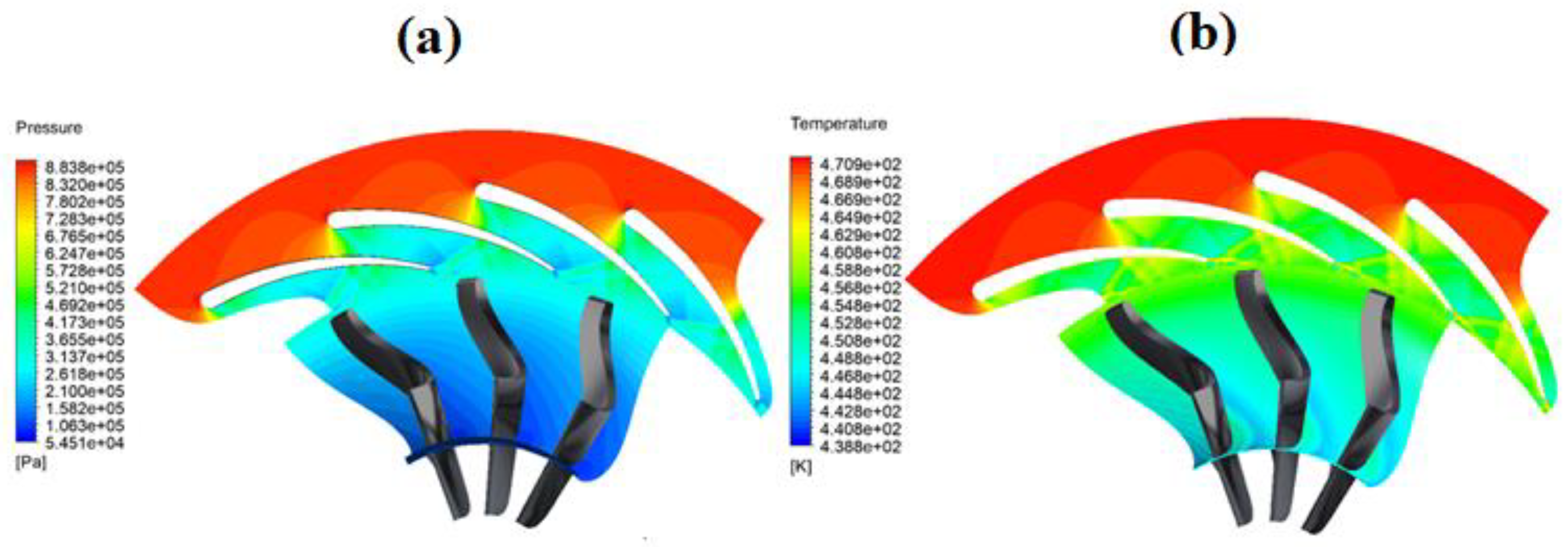
The results in this section are based on the boundary conditions presented in Table 1. Figure 18 depicts the contours of the total pressure and temperature through the turbine stage at a span of 50%. From the inlet of the stator to the exit of the rotor, the pressure decreases from 900 kPa to 130 kPa, while the temperature decreases from 471 K to 448 K. The pressure drop through the turbine stage satisfies the expansion requirement of the design point.
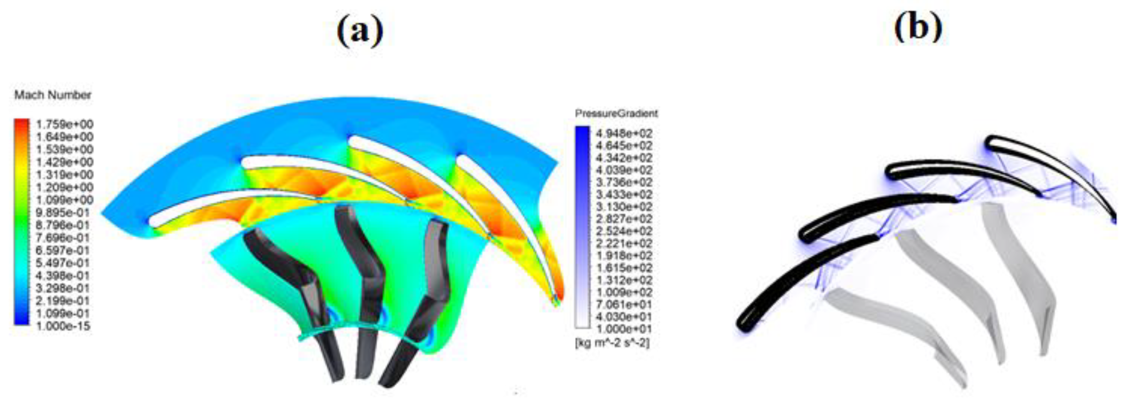
However, the high-pressure ratio results in high Mach number values at the stator exit and high loading on the turbine blades, resulting in higher friction losses and, therefore, lower efficiency, as shown in Figure 19 and Figure 20. However, this high value of Mach number is expected owing to the sudden expansion of flow at this area. Mach number is also influenced by the operating mass flow rate of the working fluid and the throat opening of the stator vanes. The pressure drop across the stator vanes is used to accelerate the organic fluid as it moves towards the circumferential direction. However, the pressure loss across the stator vane is significantly high and results in shock waves. Through the rotor blades, the values of Mach number are below unity. Figure 19 also shows the location of the shock waves, where a violent change in the pressure gradient occurred in the throat area. It is worth mentioning that the modelling approach accounting for the high Mach number values is presented in [31].
Figure 20 shows the blade loading. As the enclosed area by the pressure and suction surfaces increases, the turbine produces higher power output (net torque). At the three profiles, blade loading is uniform in the pressure and suction surfaces. The lower pressure values in the suction surface correspond to the location of the throat, where the area is the lowest and speed is the highest.
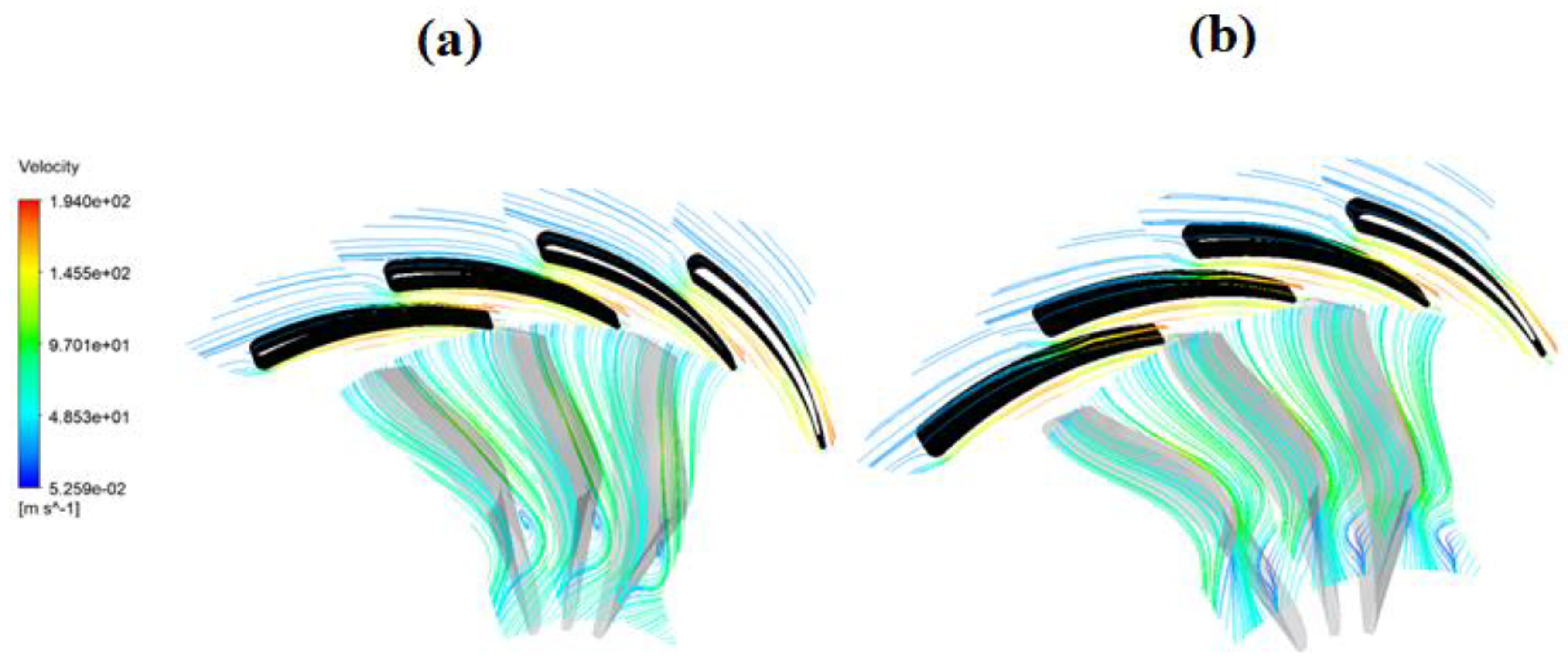
Flow recirculation is a common phenomenon in ORC turbines due to the high loading on the turbine blades. Figure 21 portrays the flow streamlines through the turbine stage. The fluid flows smoothly, and the velocity is homogenously distributed along the blade without any flow reversals at a span of 90%. The flow is smooth at the leading edge at a span of 50%, signifying that the incidence angle at the rotor leading edge is optimum. However, flow recirculation is observed downstream of the rotor blades at the suction side, resulting in a moderate level of diffusion at this area. Such flow recirculation occurs due to the difference between the actual and idealised flows in the blade passage. The fluid velocities in the end-wall boundary layers are lower than those of the mainstream, thereby causing the fluid to turn sharply and resulting in flow vortices. This indicates that this part of the blade needs to be further optimized.
6.1.3. Results at Off-Design Points
To evaluate the performance of the turbine at off-design conditions, the pressure ratio is varied from 3 to 6.9, and the turbine inlet temperature is varied from 400 K to 471.55 K, for two-speed lines (30,000 rpm and 40,000 rpm).
- Different Pressure ratios and Rotational Speeds
Mach number of the flow crucially influences the aerodynamic behaviour of turbines. It depends on the rotational speed, pressure ratio through the stage, and speed of sound of the working fluid. The results in the previous sub-section indicated that the flow choked at the interspace (the gap between stator and rotor). This means that the turbine operates at a fixed mass flow rate, regardless of the pressure ratio. This, in turn, results in shock waves and performance deterioration of the turbine. However, higher values of specific power are achieved at choked flow. Therefore, the turbine is designed to operate at choked conditions based on the simulation of the thermodynamic cycle. In the current CFD simulations, pressure ratio and turbine speed are under the control of the designer. For each run, they are changed and the simulation is re-run as shown in the next paragraphs.
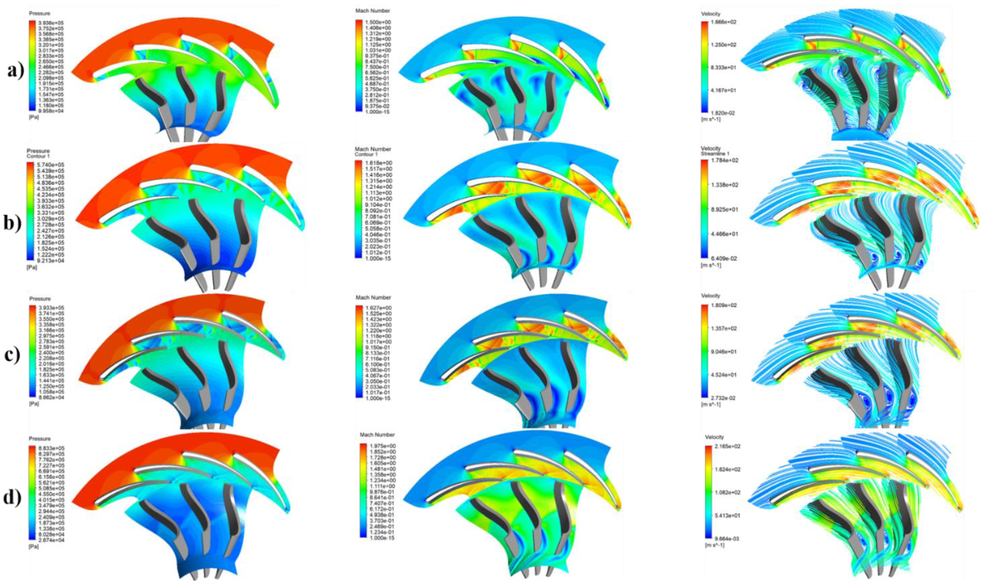
Figure 22 presents temperature distribution, Mach number distribution, and velocity streamlines through the turbine stage for different pressure ratios and rotational speeds. At PR = 3 and 40,000 rpm, Figure 22a clearly shows that there is no choking at the interspace between the stator exit and rotor inlet, and the Mach number at this region is lower than 0.93. However, running the turbine at off-design points results in a non-optimum turbine performance which results in deficient flow as depicted by the velocity streamlines in the figure. At 50% of the rotor blade, a flow recirculation is formed at the rotor leading edge in the pressure side (Figure 22a), because of the non-optimum incidence angle, before mixing out with the mainstream. The pressure ratio is then increased to 4.5 while the rotational speed is maintained constant. As shown in Figure 22b, Mach number increases significantly compared to PR = 3, reaching sonic condition (Ma = 1). Moreover, strong vortices are created downstream of the blade suction surface.
The simulation is then re-run again at two different pressure ratios ( with 30,000 rpm as shown in Figure 22c,d. It is known that turbine size is inversely proportional to the turbine speed. Therefore, the turbine size with 30,000 rpm is considered overestimated which makes the flow does not follow the blade passage properly as shown in Figure 22c,d. Mach numbers in these cases are higher than that in Figure 22a,b, although they have the same pressure ratio. However, this is justified by the higher absolute velocities. Figure 22d presents the results at and 30,000 rpm. Compared to the 40,000 rpm (Figure 22a), Mach numbers are higher due to the higher velocities as shown by the streamlines. In addition, the flow is more uniform in the 40,000 rpm case while strong vorticity is created in the 30,000 rpm.
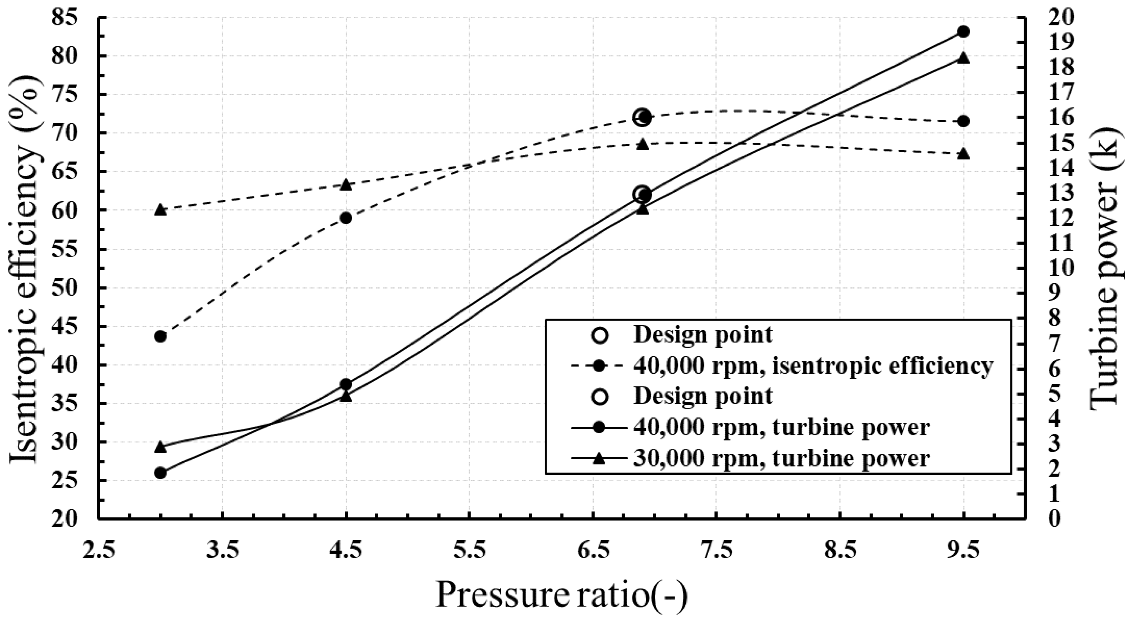
A parametric study is performed using ANSYS CFX to evaluate the turbine isentropic efficiency and power output at different pressure ratios and rotational speeds. The results are presented in Figure 23. It is clearly shown that the turbine operates more efficiently at off-design speeds 30,000 rpm than the design point 40,000 rpm at low pressure ratios. However, this is expected since the turbine is designed to operate under high-pressure ratios, which clarifies the high turbine efficiencies at high-pressure ratios. Figure 23 also shows that turbine efficiency increases with increasing the pressure ratio, reaching a maximum value and then decreases. The turbine power, on the other hand, is a function of the enthalpy drop and turbine speed, Equation (4). As shown in Figure 23, turbine power increases significantly with increasing the pressure ratio due to the increased enthalpy drop.
- Different Turbine Inlet Temperatures
Temperatures of exhaust gases in an internal combustion engine vary considerably according to vehicle’s operation. As mentioned in the previous study [14], the turbine inlet temperature increases linearly with increasing heat source temperature. Therefore, turbine performance is also investigated at different inlet temperatures and rotational speeds in the current study.
Like the design point, flow vortices are noticed downstream of the rotor blades at the suction side for all off-design points, as shown in Figure 24. This indicates that this part of the blade is not optimum. Figure 24 also indicates that flow pattern improves with increasing turbine inlet temperature for the same rotational speed. The closer inlet temperature gets to design point, the more uniform flow results as shown in Figure 24a,b. At off-design rotational speed (30,000 rpm), the flow is more uniform than that in design point speed (40,000) for low temperatures due to low fluid densities at the stator exit. In contrast, flow pattern improves better with 40,000 rpm than 30,000 rpm at high temperatures since the fluid density at the stator exit is 33% lower.
Figure 24 shows also that the Mach number at stator exit increases with increasing the turbine inlet temperature for the same rotational speed. Mach number is a function of flow absolute velocity and speed of sound. As temperature increases, flow velocity increases resulting in higher Mach number. Compared to Figure 24d, Mach number in Figure 24c decreases by 19.74% since the absolute velocity decreases by 31.87%. Figure 24 shows also that Mach number decreases with increasing rotational speed for the same temperature and pressure ratio, according to the flow velocity. At 30,000 rpm (Figure 24c), the flow velocity at the stator exit is 20.80% higher than that at 40,000 rpm (Figure 24a). The relationship between flow velocity and rotational speed is explained in the velocity triangle in a previous study [31]. Lowering the rotor rotational speed results in higher tangential velocity in the interspace which results in higher absolute velocity, and consequently, higher Mach number.
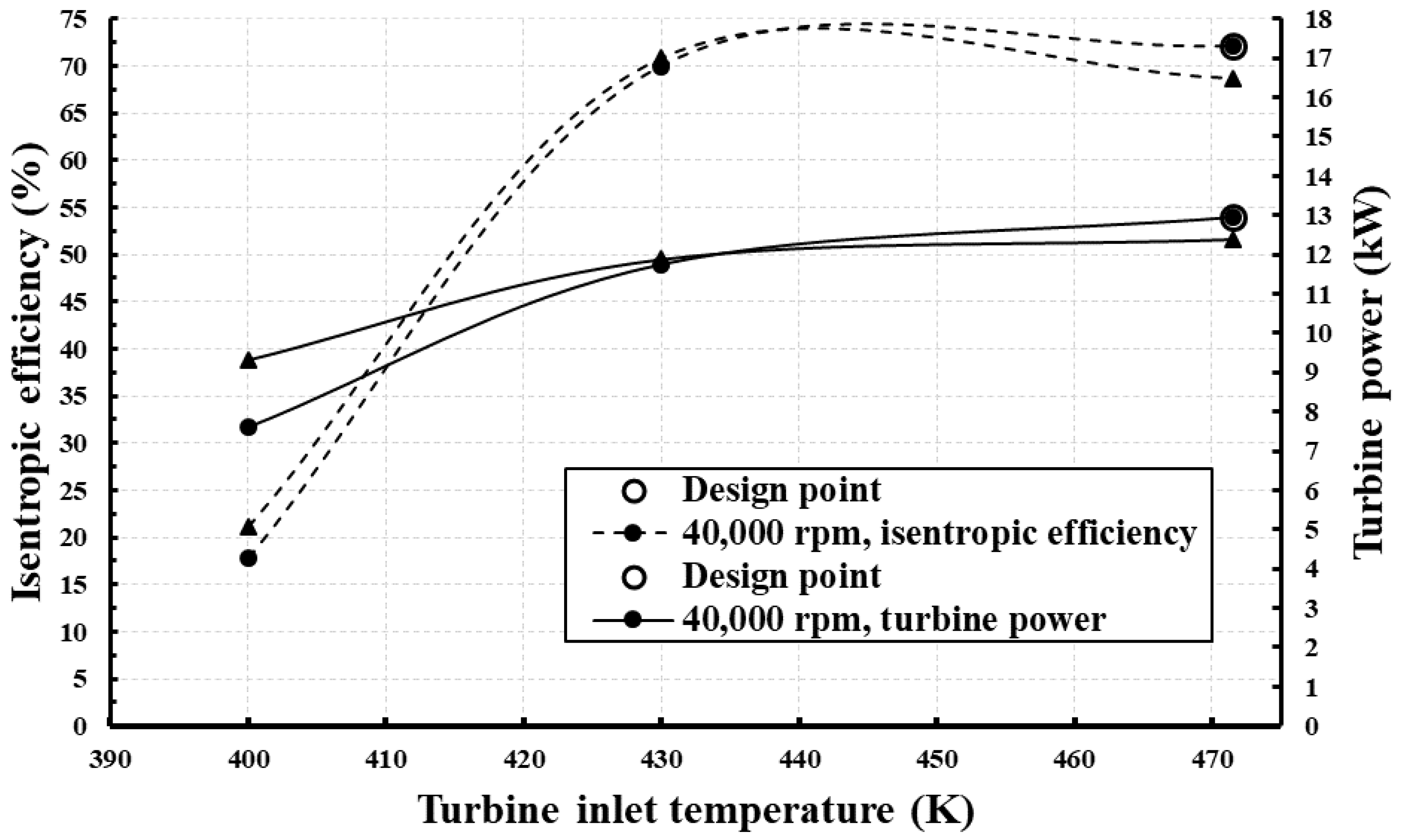
Turbine performance is explored at different turbine inlet temperatures and rotational speeds as shown in Figure 25. For the design point speed, turbine efficiency increases with increasing inlet temperature, reaching a maximum value at the design point inlet temperature (471.55 K). For the 30,000 rpm, turbine efficiency decreases linearly with increasing inlet temperature. At 430 K, enthalpy drop with 30,000 rpm is higher than that in 40,000 rpm clarifying the higher efficiency and power output at this point. As the temperature increase, the enthalpy drop with 40,000 rpm becomes higher which results in higher turbine efficiency and power output. Figure 25 shows also that turbine efficiency decreases with increasing turbine inlet temperature for 30,000 rpm. This is due to the flow deficiency downstream of the rotor blades at the suction side. Although flow vortices are created in both cases (Figure 24c,d), the latter results in lower flow velocity (compared to the upstream flow) which increases the strength of the vortices and consequently lower turbine efficiency.
6.2. Comparison between the Mean-Line Model and CFD Results
One of the main aims of the CFD simulation at the design point is to validate the mean-line model as presented in Table 6. ANSYS provides a summary of the mass averaged solution variables (total pressure, total temperature and static temperature), area-averaged solution variables (static pressure and velocities), and derived quantities (as total to static efficiency and power output). These variables are computed at the inlet and exit of each component of the turbine, as shown in Table 6. Such variables are selected as the comparison variables between the 1D and 3D simulations.
As seen in Table 6, the majority of the 1D parameters are in excellent agreement with 3D simulations. Maximum deviations of 15.39% can be noticed in rotor exit absolute velocity. This is justified by the assumption of the isentropic flow through the stator as shown in [31]. As a result, at a fixed mass flow rate, the meridional velocity, , increases to conserve the mass flow rate. This increase in the meridional velocity results in higher absolute velocity, and consequently, higher deviation in rotor relative velocity, . This is not the case in the CFD analysis where the stagnation pressure drop in the stator is considered; therefore, the flow is not isentropic as shown in Figure 18. The deviation in the turbine efficiency and work output are 2.28% and 5.10%, respectively. Overall, the CFD results indicate that the proposed 1D design methodology can accurately predict the turbine performance and flow features for high-pressure ratio ORC radial inflow turbines.
6.3. Results of the ORC System
Results of ORC System at Design and Off-Design Conditions
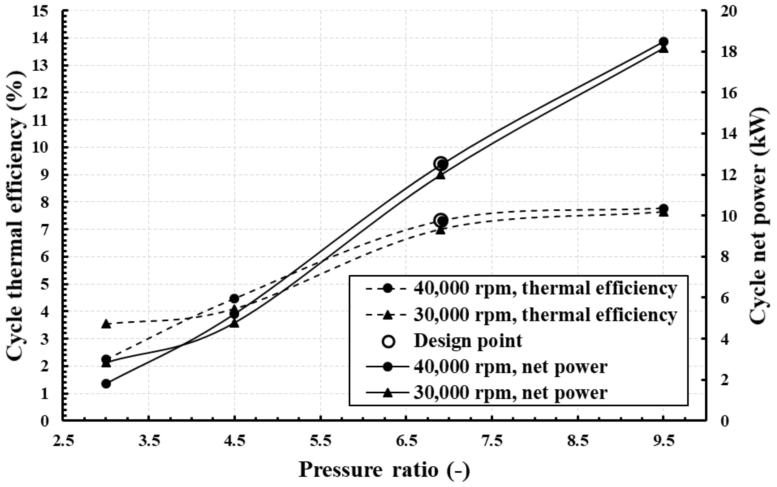
The effects of turbine operating conditions on cycle thermal efficiency and net power are also investigated as shown in Figure 26 and Figure 27. Increasing the pressure ratio results in higher cycle network due to the increased turbine power as discussed in Figure 23 Similarly, cycle efficiency increases as turbine pressure ratio increases. It is worth mentioning that cycle optimum point differs from the turbine one. The former is obtained at a pressure ratio equal to 9.5 while the latter results at a pressure ratio equal to 6.9. Cycle efficiency is a function of cycle net power that increases with increasing turbine pressure ratio.
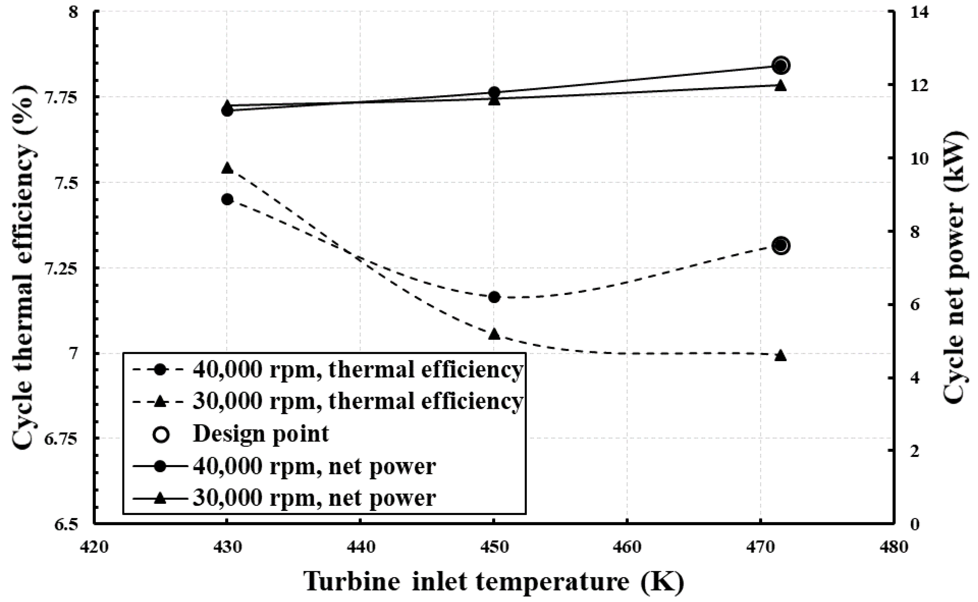
Figure 27 shows that cycle net power increases linearly with increasing turbine inlet temperature because of the increased turbine power, Figure 25. The cycle thermal efficiency, on the other hand, shows different trends. For 40,000 rpm, it decreases with increasing inlet temperature then increases, reaching the design point. For 30,000 rpm, the cycle efficiency decreases with increasing temperature. The different trend in both speeds is related to the definition of the cycle thermal efficiency. Cycle thermal efficiency is a function of cycle net power divided by heat input. The heat input increases with increasing the inlet temperature. For 30,000 rpm, the rate of increase of heat input is greater than that of cycle net power for all operating temperatures. For 40,000 rpm, on the other hand, the rate of increase of heat input from 430 to 450 K is 8.60% compared 4.17% of net power. From 450 to 471.55 K, the rate of increase in heat input is 4.07% compared to 5.80% of net power. This clarifies the trend of cycle thermal efficiency operating with 40,000 rpm.
6.4. Results of Finite Element Analyses (FEA)
For safe operation, the maximum von Mises stress and stress and total displacement should not exceed be the material tensile strength and the tip clearance gap between the rotor and casing. Figure 28 presents the results of the FEA at the design point using Fullcure 720. In addition, Table 7 summarizes the FEA at design and off-design points for the considered types of material. As can be seen in Figure 28, the maximum stress and deformation due to fluid pressure are 0.54 MPa and 0.001 mm which are well below the limits (60 MPa and 0.6 mm). However, it is apparent from Table 7 that maximum stress and deformation due to rotation increase significantly. Although the maximum stress (29.22 MPa) is still below the material tensile strength, the deformation at the blade tip is 0.48 mm which is very close to the assigned clearance gap (0.6 mm). Therefore, although Fullcure 720 is cost-effective, using such material in the current application is risky due to the possibility of metal fusion near the blade tip. It is evident from Figure 28 that the maximum stress occurs at the blade root in the hub for both fluid pressure and rotation. The maximum deformation, on the other hand, occurs at the at exit tip for both fluid pressure and rotation. Similar locations of maximum stress and deformation are also noticed for all considered types of materials and with different operating conditions (i.e., off-design operation). It is worth mentioning that the locations of maximum stress and deformation agree with locations mentioned in Moustapha et al. [68]. For other types of material, the maximum stress and deformation are well below limits for both fluid pressure and rotation.
At off-design operations, similar observations are noticed. However, reducing the rotational speed from 40,000 to 30,000 rpm results in lower blade tip deformation (0.27 mm compared to 0.48 mm). Table 7 also indicates that stainless steel is not appropriate for the current application due to high resulted stress. Therefore, the best option for the current application is either a titanium alloy or aluminium alloy. However, titanium alloy is typically 20 times more expensive than a corresponding aluminium part [69].
7. Conclusions
This paper presented the fluid–structure interaction of a high pressure-ratio backswept radial inflow turbine operating with high-dense working fluid at design and off-design points. The main conclusions of the current study are summarized below:
- The proposed mathematical modelling for generating 3D shapes of turbine blades and vanes is fast and accurate.
- The CFD simulations indicated the robustness of the proposed 1D mean-line model. The deviations between the 1D mean-line and 3D CFD in turbine efficiency and power output were 2.28% and 5.10%, respectively. In addition, the 3D CFD results confirmed the optimum blade angle value optimized by the 1D mean-line model.
- At the design point, the flow at the stator exit was supersonic as expected. However, it was smooth with no flow-vortices. In the rotor blades, the fluid was flowing smoothly, and the velocity was homogenously distributed at 90% span. At the 50% span, flow recirculation was observed downstream of the rotor blades at the suction side, resulting in a moderate level of diffusion at this area. The results also indicated that the curvature downstream the blade should be optimized.
- At off-design conditions, the performance of the turbine was non-optimum. In addition, strong flow vortices resulted in the passage of the rotor blade. Increasing the stage pressure ratio resulted in high Mach numbers which negatively affected the turbine performance while affected the output power positively. For low turbine inlet temperatures, the flow is more uniform at 30,000 rpm than that in design point speed (40,000 rpm). In contrast, flow pattern improves better with 40,000 rpm than 30,000 rpm at high temperatures since the fluid density at the stator exit is lower.
- The FEA indicated that material selection is a trade-off between its mechanical integrity and cost. Fullcure 720 should be avoided in the current application due to the possibility of metal fusion near the blade tip. Similarly, stainless steel is not appropriate for the current application due to high resulted stress. Titanium alloy and aluminium alloy can be used for the current applications, although the former is typically 20 times more expensive.
- Cycle thermal efficiency and net power were investigated at various pressure ratios and turbine inlet temperatures. As pressure ratio increases, cycle thermal efficiency and net power increases due to the increased turbine power output. The results also indicated that cycle net power increases linearly with increasing turbine inlet temperature while cycle thermal efficiency showed different trends according to the rotational speed.
Author Contributions
Conceptualization, F.A. and A.P.; methodology, F.A. and M.E.; software, F.A.; validation, A.P., M.E. and F.A.; formal analysis, M.E.; investigation, A.P. and F.A.; resources, A.P.; data curation, M.E.; writing—original draft preparation, F.A.; writing—review and editing, A.P. and M.E.; visualization, F.A.; supervision, A.P.; project administration, A.P. and F.A.; funding acquisition A.P. All authors have read and agreed to the published version of the manuscript.
Funding
This research was funded by Innovate UK, grant number TS/M012220/1.
Conflicts of Interest
The authors declare no conflict of interest.
Nomenclature
| 1–5 | Stations through turbine | Subscript | |
| a | Speed of sound (m/s) | h | hub |
| A | Area | hyd | hydraulic |
| b | blade height (m) | r | radial, rotor |
| C | Absolute velocity (m/s) | rms | root mean square |
| Cθ | Tangential velocity (m/s) | s | insentropic, stator |
| d | diameter (m) | t | tip, total |
| h | Enthalpy (kJ/kg) | x | axial |
| Ma | Mach number (-) | Greek Symbols | |
| m’ | Mass flow rate (kg/s) | η | Efficiency (-) |
| N | Rotational speed (RPM) | β | Relative angle (deg) |
| P | Pressure (kPa) | ρ | Density (kg/m3) |
| r | radius (m) | α | Absolute flow angle (deg) |
| s | Entropy (kJ/kg·k) | Setting angle | |
| T | Temperature (K) | Azimuth angle | |
| U | Tip speed (m/s) | Abbreviations | |
| w | Relative velocity (m/s) | BSFC | Break specific fuel consumption |
| W | work (kW) | CFD | Computational fluid dynamics |
| z | Axial length (m) | EoS | Equation of state |
| HCCI | homogeneous charge compression ignition | ||
| ICE | Internal combustion engine | ||
| NOx | Nitrogen Oxide | ||
| ORC | Organic Ranke cycle | ||
| PM | Particulate matter | ||
| WHR | Waste heat recovery |
References
- Climate Change: How Do We Know? Available online: https://climate.nasa.gov/evidence/ (accessed on 12 April 2020).
- Xu, W.; Zhao, L.; Mao, S.S.; Deng, S. Towards novel low temperature thermodynamic cycle: A critical review originated from organic Rankine cycle. Appl. Energy 2020, 270, 115186. [Google Scholar] [CrossRef]
- Energy Use for Transportation. 2018. Available online: https://www.eia.gov/energyexplained/use-of-energy/transportation.php (accessed on 23 April 2020).
- Sub-national Road Transport Consumption Data. Available online: https://www.gov.uk/government/collections/road-transport-consumption-at-regional-and-local-level (accessed on 19 April 2020).
- PETROLEUM & OTHER LIQUIDS. 2020. Available online: https://www.eia.gov/dnav/pet/pet_pri_gnd_dcus_nus_w.htm (accessed on 20 April 2020).
- Liu, L.; Wang, K.; Wang, S.; Zhang, R.; Tang, X. Assessing energy consumption, CO2 and pollutant emissions and health benefits from China’s transport sector through 2050. Energy Policy 2018, 116, 382–396. [Google Scholar] [CrossRef]
- Qiu, K.; Entchev, E. Development of an organic Rankine cycle-based micro combined heat and power system for residential applications. Appl. Energy 2020, 275, 115335. [Google Scholar] [CrossRef]
- Hoang, A.T. Waste heat recovery from diesel engines based on Organic Rankine Cycle. Appl. Energy 2018, 231, 138–166. [Google Scholar] [CrossRef]
- Karvountzis-Kontakiotis, A.; Pesiridis, A.; Zhao, H.; Alshammari, F.; Franchetti, B.; Pesmazoglou, I.; Tocci, L. Effect of an ORC Waste Heat Recovery System on Diesel Engine Fuel Economy for Off-Highway Vehicles. SAE Tech. Pap. Ser. 2017. [Google Scholar] [CrossRef]
- Srinivasan, K.K.; Mago, P.J.; Krishnan, S.R. Analysis of exhaust waste heat recovery from a dual fuel low temperature combustion engine using an Organic Rankine Cycle. Energy 2010, 35, 2387–2399. [Google Scholar] [CrossRef]
- Karvountzis-Kontakiotis, A.; Alshammari, F.; Pesiridis, A.; Franchetti, B.; Pesmazoglou, I.; Tocci, L. Variable Geometry Turbine Design for Off-Highway Vehicle Organic Rankine Cycle Waste Heat Recovery. In Proceedings of the THIESEL 2016 Conference on Thermo-and Fluid Dynamic Processes in Direct Injection Engines, Valencia, Spain, 13–16 September 2016. [Google Scholar]
- Zhang, Y.; Wu, Y.-T.; Xia, G.-D.; Ma, C.-F.; Ji, W.-N.; Liu, S.-W.; Yang, K.; Yang, F. Development and experimental study on organic Rankine cycle system with single-screw expander for waste heat recovery from exhaust of diesel engine. Energy 2014, 77, 499–508. [Google Scholar] [CrossRef]
- Guillaume, L.; Legros, A.; Wronski, J.; Lemort, V. Performance of a radial-inflow turbine integrated in an ORC system and designed for a WHR on truck application: An experimental comparison between R245fa and R1233zd. Appl. Energy 2017, 186, 408–422. [Google Scholar] [CrossRef]
- Alshammari, F.; Pesyridis, A.; Karvountzis-Kontakiotis, A.; Franchetti, B.; Pesmazoglou, Y. Experimental study of a small scale organic Rankine cycle waste heat recovery system for a heavy duty diesel engine with focus on the radial inflow turbine expander performance. Appl. Energy 2018, 215, 543–555. [Google Scholar] [CrossRef]
- Alshammari, F.; Pesyridis, A. Experimental study of organic Rankine cycle system and expander performance for heavy-duty diesel engine. Energy Convers. Manag. 2019, 199, 111998. [Google Scholar] [CrossRef]
- Lion, S.; Taccani, R.; Vlaskos, I.; Scrocco, P.; Vouvakos, X.; Kaiktsis, L. Thermodynamic analysis of waste heat recovery using Organic Rankine Cycle (ORC) for a two-stroke low speed marine Diesel engine in IMO Tier II and Tier III operation. Energy 2019, 183, 48–60. [Google Scholar] [CrossRef]
- Imran, M.; Haglind, F.; Lemort, V.; Meroni, A. Optimization of organic rankine cycle power systems for waste heat recovery on heavy-duty vehicles considering the performance, cost, mass and volume of the system. Energy 2019, 180, 229–241. [Google Scholar] [CrossRef]
- Nawi, Z.M.; Kamarudin, S.; Abdullah, S.S.; Lam, S. The potential of exhaust waste heat recovery (WHR) from marine diesel engines via organic rankine cycle. Energy 2019, 166, 17–31. [Google Scholar] [CrossRef]
- Ezoji, H.; Ajarostaghi, S.S.M. Thermodynamic-CFD analysis of waste heat recovery from homogeneous charge compression ignition (HCCI) engine by Recuperative organic Rankine Cycle (RORC): Effect of operational parameters. Energy 2020, 205, 117989. [Google Scholar] [CrossRef]
- Yue, C.; Tong, L.; Zhang, S. Thermal and economic analysis on vehicle energy supplying system based on waste heat recovery organic Rankine cycle. Appl. Energy 2019, 248, 241–255. [Google Scholar] [CrossRef]
- Liao, G.; E, J.; Zhang, F.; Chen, J.; Leng, E. Advanced exergy analysis for Organic Rankine Cycle-based layout to recover waste heat of flue gas. Appl. Energy 2020, 266, 114891. [Google Scholar] [CrossRef]
- Liu, X.; Nguyen, M.Q.; Chu, J.; Lan, T.; He, M.-G. A novel waste heat recovery system combing steam Rankine cycle and organic Rankine cycle for marine engine. J. Clean. Prod. 2020, 265, 121502. [Google Scholar] [CrossRef]
- Le Brun, N.; Simpson, M.; Acha, S.; Shah, N.; Markides, C.N. Techno-economic potential of low-temperature, jacket-water heat recovery from stationary internal combustion engines with organic Rankine cycles: A cross-sector food-retail study. Appl. Energy 2020, 274, 115260. [Google Scholar] [CrossRef]
- Ochoa, G.V.; Prada, G.; Duarte-Forero, J. Carbon footprint analysis and advanced exergo-environmental modeling of a waste heat recovery system based on a recuperative organic Rankine cycle. J. Clean. Prod. 2020, 274, 122838. [Google Scholar] [CrossRef]
- Palagi, L.; Sciubba, E.; Tocci, L. A neural network approach to the combined multi-objective optimization of the thermodynamic cycle and the radial inflow turbine for Organic Rankine cycle applications. Appl. Energy 2019, 237, 210–226. [Google Scholar] [CrossRef]
- Alshammari, M.; Alshammari, F.; Pesyridis, A. Electric Boosting and Energy Recovery Systems for Engine Downsizing. Energies 2019, 12, 4636. [Google Scholar] [CrossRef] [Green Version]
- Aungier, R.H. Turbine Aerodynamics: Axial-Flow and Radial-Inflow Turbine Design and Analysis, 1st ed.; ASME: New York, NY, USA, 2006. [Google Scholar]
- Da Lio, L.; Manente, G.; Lazzaretto, A. A mean-line model to predict the design efficiency of radial inflow turbines in organic Rankine cycle (ORC) systems. Appl. Energy 2017, 205, 187–209. [Google Scholar] [CrossRef]
- Zou, A.; Chassaing, J.-C.; Persky, R.; Gu, Y.T.; Sauret, E. Uncertainty Quantification in high-density fluid radial-inflow turbines for renewable low-grade temperature cycles. Appl. Energy 2019, 241, 313–330. [Google Scholar] [CrossRef]
- Song, H.; Zhang, J.; Huang, P.; Cai, H.; Cao, P.; Hu, B. Analysis of Rotor-Stator Interaction of a Pump-Turbine with Splitter Blades in a Pump Mode. Mathematics 2020, 8, 1465. [Google Scholar] [CrossRef]
- Alshammari, F.; Karvountzis-Kontakiotis, A.; Pesyridis, A.; Alatawi, I. Design and study of back-swept high pressure ratio radial turbo-expander in automotive organic Rankine cycles. Appl. Therm. Eng. 2020, 164, 114549. [Google Scholar] [CrossRef]
- Nguyen, D.V.; Jansson, J.; Goude, A.; Hoffman, J. Direct Finite Element Simulation of the turbulent flow past a vertical axis wind turbine. Renew. Energy 2019, 135, 238–247. [Google Scholar] [CrossRef]
- Colonna, P.; Rebay, S.; Harinck, J.; Guardone, A. Real-Gas Effects in ORC Turbine Flow Simulations: Influence of Thermodynamic Models on Flow Fields and Performance Parameters. In Proceedings of the ECCOMAS CFD 2006: Proceedings of the European Conference on Computational Fluid Dynamics, Egmond aan Zee, The Netherlands, 5–8 September 2006. [Google Scholar]
- Harinck, J.; Pasquale, D.; Pecnik, R.; Van Buijtenen, J.; Colonna, P. Performance improvement of a radial organic Rankine cycle turbine by means of automated computational fluid dynamic design. Proc. Inst. Mech. Eng. Part A J. Power Energy 2013, 227, 637–645. [Google Scholar] [CrossRef]
- Lemmon, E.W.; Huber, M.L.; McLinden, M.O. NIST Standard Reference Database 23: Reference Fluid Thermodynamic and Transport Properties-REFPROP, Version 9.0; National Institute of Standards and Technology, Standard Reference Data Program: Gaithersburg, MA, USA, 2010. [Google Scholar]
- Sauret, E.; Gu, Y. Three-dimensional off-design numerical analysis of an organic Rankine cycle radial-inflow turbine. Appl. Energy 2014, 135, 202–211. [Google Scholar] [CrossRef] [Green Version]
- Uusitalo, A.; Turunen-Saaresti, T.; Guardone, A.; Grönman, A. Design and Flow Analysis of a Supersonic Small Scale ORC Turbine Stator with High Molecular Complexity Working Fluid. Vol. 2D Turbomach. 2014. [Google Scholar] [CrossRef]
- White, M. The Design and Analysis of Radial Inflow Turbines Implemented within Low Temperature Organic Rankine Cycles. Ph.D. Thesis, City University London, London, UK, 2015. [Google Scholar]
- Verma, R.; Sam, A.; Ghosh, P. CFD Analysis of Turbo Expander for Cryogenic Refrigeration and Liquefaction Cycles. Phys. Procedia 2015, 67, 373–378. [Google Scholar] [CrossRef] [Green Version]
- Nithesh, K.; Chatterjee, D. Numerical prediction of the performance of radial inflow turbine designed for ocean thermal energy conversion system. Appl. Energy 2016, 167, 1–16. [Google Scholar] [CrossRef]
- Song, Y.; Sun, X.; Huang, D. Preliminary design and performance analysis of a centrifugal turbine for Organic Rankine Cycle (ORC) applications. Energy 2017, 140, 1239–1251. [Google Scholar] [CrossRef]
- Daabo, A.M.; Mahmoud, S.; Al-Dadah, R.; Al Jubori, A.M.; Ennil, A.B. Numerical analysis of small scale axial and radial turbines for solar powered Brayton cycle application. Appl. Therm. Eng. 2017, 120, 672–693. [Google Scholar] [CrossRef]
- Dong, B.; Xu, G.; Li, T.; Quan, Y.; Zhai, L.; Wen, J. Numerical prediction of velocity coefficient for a radial-inflow turbine stator using R123 as working fluid. Appl. Therm. Eng. 2018, 130, 1256–1265. [Google Scholar] [CrossRef]
- Sun, W.; Chen, S.; Hou, Y.; Bu, S.; Ma, Z.; Zhang, L.; Pan, L. Numerical studies on two-phase flow in cryogenic radial-inflow turbo-expander using varying condensation models. Appl. Therm. Eng. 2019, 156, 168–177. [Google Scholar] [CrossRef]
- Wang, Z.; Zhang, Z.; Xia, X.; Zhao, B.; He, N.; Peng, D. Preliminary design and numerical analysis of a radial inflow turbine in organic Rankine cycle using zeotropic mixtures. Appl. Therm. Eng. 2019, 162, 114266. [Google Scholar] [CrossRef]
- Schuster, S.; Markides, C.N.; White, A.J. Design and off-design optimisation of an organic Rankine cycle (ORC) system with an integrated radial turbine model. Appl. Therm. Eng. 2020, 174, 115192. [Google Scholar] [CrossRef]
- Al Jubori, A.M.; Al-Mousawi, F.N.; Rahbar, K.; Al-Dadah, R.; Mahmoud, S. Design and manufacturing a small-scale radial-inflow turbine for clean organic Rankine power system. J. Clean. Prod. 2020, 257, 120488. [Google Scholar] [CrossRef]
- Zhang, F.; Zhu, L.; Chen, K.; Yan, W.; Appiah, D.; Hu, B. Numerical Simulation of Gas–Liquid Two-Phase Flow Characteristics of Centrifugal Pump Based on the CFD–PBM. Mathematics 2020, 8, 769. [Google Scholar] [CrossRef]
- Vlase, S.; Nicolescu, A.E.; Marin, M. New Analytical Model Used in Finite Element Analysis of Solids Mechanics. Mathematics 2020, 8, 1401. [Google Scholar] [CrossRef]
- Wang, W.; Zhang, H.; Liu, P.; Li, Z.; Ni, W.; Uechi, H.; Matsumura, T. A finite element method approach to the temperature distribution in the inner casing of a steam turbine in a combined cycle power plant. Appl. Therm. Eng. 2016, 105, 18–27. [Google Scholar] [CrossRef]
- Chen, L.-J.; Xie, L.-Y. Prediction of high-temperature low-cycle fatigue life of aeroengine’s turbine blades at low-pressure stage. J. Northeast. Univ. 2005, 26, 673–676. [Google Scholar]
- Fu, N. Strength Analysis and Life Calculation of a Typical Aeronautical Engine Turbine Disc and Blade. Ph.D. Thesis, Northwestern Polytechnical University, Xi’an, China, 2006. [Google Scholar]
- Odabaee, M.; Shanechi, M.M.; Hooman, K. CFD simulation and FE analysis of a high pressure ratio radial inflow turbine. In Proceedings of the 19AFMC: 19th Australasian Fluid Mechanics Conference, Melbourne, Australia, 8–11 December 2014. [Google Scholar]
- Gad-El-Hak, I. Fluid⁻Structure Interaction for Biomimetic Design of an Innovative Lightweight Turboexpander. Biomimetics 2019, 4, 27. [Google Scholar] [CrossRef] [Green Version]
- Xie, Y.; Lu, K.; Liu, L.; Xie, G. Fluid-Thermal-Structural Coupled Analysis of a Radial Inflow Micro Gas Turbine Using Computational Fluid Dynamics and Computational Solid Mechanics. Math. Probl. Eng. 2014, 2014, 1–10. [Google Scholar] [CrossRef]
- Banaszkiewicz, M. On-line monitoring and control of thermal stresses in steam turbine rotors. Appl. Therm. Eng. 2016, 94, 763–776. [Google Scholar] [CrossRef]
- Wang, Z.; Ding, S.; Li, G. Failure risk control for aeroengine turbine disks based on active thermal management. Appl. Therm. Eng. 2017, 120, 367–377. [Google Scholar] [CrossRef]
- Atkinson, M.J. The Design of Efficient Radial Turbines for Low Power Applications. Ph.D. Thesis, University of Sussex, Brighton, UK, 1998. [Google Scholar]
- ANSYS Inc. ANSYS CFX-Solver Theory Guide, Release 18.0; ANSYS Inc.: Canonsburg, PA, USA, 2018. [Google Scholar]
- Fajardo, D.P. Methodology for the Numerical Characterization of a Radial Turbine under Steady and Pulsating Flow. Ph.D. Thesis, Universitat Politecnica De Valencia, Valencia, Spain, 2012. [Google Scholar]
- Menter, F.R. Two-equation eddy-viscosity turbulence models for engineering applications. AIAA J. 1994, 32, 1598–1605. [Google Scholar] [CrossRef] [Green Version]
- Bahr Ennil, A. Optimization of Small-Scale Axial Turbine for Distributed Compressed Air Energy Storage System. Ph.D. Thesis, University of Birmingham, Birmingham, UK, 2016. [Google Scholar]
- Kim, J.-S.; Kim, D.-Y.; Kim, Y. Experiment on radial inflow turbines and performance prediction using deep neural network for the organic Rankine cycle. Appl. Therm. Eng. 2019, 149, 633–643. [Google Scholar] [CrossRef]
- Kang, S.H. Design and experimental study of ORC (organic Rankine cycle) and radial turbine using R245fa working fluid. Energy 2012, 41, 514–524. [Google Scholar] [CrossRef]
- Kaczmarczyk, T.Z.; Żywica, G.; Ihnatowicz, E. Experimental study of a low-temperature micro-scale organic Rankine cycle system with the multi-stage radial-flow turbine for domestic applications. Energy Convers. Manag. 2019, 199, 111941. [Google Scholar] [CrossRef]
- Linnemann, M.; Priebe, K.-P.; Heim, A.; Wolff, C.; Vrabec, J. Experimental investigation of a cascaded organic Rankine cycle plant for the utilization of waste heat at high and low temperature levels. Energy Convers. Manag. 2020, 205, 112381. [Google Scholar] [CrossRef] [Green Version]
- Alshammari, F. Radial Turbine Expander Design, Modelling and Testing for Automotive Organic Rankine Cycle Waste Heat Recovery. Ph.D. Thesis, Brunel University, London, UK, 2018. [Google Scholar]
- Moustapha, H.; Zelesky, M.F.; Baines, N.C.; Japikse, D. Axial and Radial Turbines, 1st ed.; Concepts ETI, Inc.: White River Junction, VT, USA, 2003. [Google Scholar]
- U.S Department of Energy. Low-Cost Titanium Alloy Production. 2016. Available online: https://www.energy.gov/sites/prod/files/2016/08/f33/LowCostTitaniumAlloyProduction_0.pdf (accessed on 10 June 2020).
Figure 1.
Flowchart of the present study.

Figure 2.
Schematic of typical organic Rankine cycle (ORC) coupled internal combustion engine (ICE).
Figure 2.
Schematic of typical organic Rankine cycle (ORC) coupled internal combustion engine (ICE).

Figure 3.
Meridional view of the turbine stage.

Figure 4.
Creation of stator 3D model.

Figure 5.
Distributions of vane angle and thickness of stator.

Figure 6.
3D model of turbine stator.

Figure 7.
Meridional profiles of the turbine blade.

Figure 8.
Distribution of rotor blade angles.

Figure 9.
Definitions of blade thickness (a) and 3D model of turbine rotor blade (b).

Figure 10.
Flowchart of numerical analysis adopted.

Figure 11.
3D view of a radial turbine stage and boundary conditions.

Figure 12.
Mesh of the passage with 1.0 × 10⁶ elements.

Figure 13.
Mesh independence study using ANSYS TurboGrid.

Figure 14.
Computational fluid domains for stator and rotor.

Figure 15.
Specified boundary conditions for the finite element analysis (FEA), fixed support (a) and rotational speed and its axis (b).
Figure 15.
Specified boundary conditions for the finite element analysis (FEA), fixed support (a) and rotational speed and its axis (b).

Figure 16.
FEA mesh of point 8 in Table 5.
Figure 16.
FEA mesh of point 8 in Table 5.

Figure 17.
Comparison between numerical results and experimental results.

Figure 18.
Pressure (a) and temperature (b) distributions at design point (N = 40,000 rpm, PR = 6.9).
Figure 18.
Pressure (a) and temperature (b) distributions at design point (N = 40,000 rpm, PR = 6.9).

Figure 19.
Mach number distribution (a) and pressure gradient (b) at design point (N = 40,000 rpm, PR = 6.9).
Figure 19.
Mach number distribution (a) and pressure gradient (b) at design point (N = 40,000 rpm, PR = 6.9).

Figure 20.
Blade loading through the rotor blades.

Figure 21.
Velocity streamline at 50% span (a) and 90% span (b), at design point (N = 40,000 rpm, PR = 6.9).
Figure 21.
Velocity streamline at 50% span (a) and 90% span (b), at design point (N = 40,000 rpm, PR = 6.9).

Figure 22.
Pressure distributions, Mach numbers, and velocity streamlines at 50% span and 471.55 K, for (a) PR = 3, N = 40,000 rpm (b) PR = 4.5, N = 40,000 rpm (c) PR = 3, N = 30,000 rpm and (d) PR = 6.9, N = 30,000 rpm.
Figure 22.
Pressure distributions, Mach numbers, and velocity streamlines at 50% span and 471.55 K, for (a) PR = 3, N = 40,000 rpm (b) PR = 4.5, N = 40,000 rpm (c) PR = 3, N = 30,000 rpm and (d) PR = 6.9, N = 30,000 rpm.

Figure 23.
Turbine efficiency and power output at various pressure ratios.

Figure 24.
Temperature distributions, Mach numbers, and velocity streamlines at 50% span for (a) T = 430 K, N = 40,000 rpm, (b) T = 450 K, N = 40,000 and (c) T = 430 K, N = 30,000 (d) T = 450 K, N = 30,000 rpm.
Figure 24.
Temperature distributions, Mach numbers, and velocity streamlines at 50% span for (a) T = 430 K, N = 40,000 rpm, (b) T = 450 K, N = 40,000 and (c) T = 430 K, N = 30,000 (d) T = 450 K, N = 30,000 rpm.

Figure 25.
Turbine efficiency and power output at various turbine inlet temperatures.

Figure 26.
Cycle thermal efficiency and net power at various pressure ratios.

Figure 27.
Cycle thermal efficiency and net power at various turbine inlet temperatures.

Figure 28.
Distributions of von Mises and displacement due to fluid pressure (a) and rotation (b), using Fullcure 720.
Figure 28.
Distributions of von Mises and displacement due to fluid pressure (a) and rotation (b), using Fullcure 720.


Table 1.
Mean-line and computational fluid dynamics (CFD) input conditions.
| Engine Points | P3 |
|---|---|
| Inlet total pressure, (kPa) | 900 * |
| Inlet total temperature, (K) | 471.5 * |
| Pressure ratio, PR (-) | 6.9 * |
| Rotational speed, N (rpm) | 40,000 * |
| Mass flow rate, (kg/s) | 0.8 |
| Loading coefficient, | 1.25 |
| Flow coefficient | 0.25 |
* Input conditions for CFD analysis.
Table 2.
Basic equations for turbine and ORC applied in the current study.
| Equation | Equation # | Comments |
|---|---|---|
| (1) | is the heat transfer in the evaporator in kW. and are enthalpies in kJ/kg at exit and inlet of the evaporator. is the working fluid mass flow rate in kg/s. | |
| (2) | is the power consumed by pump in kW. , , and are outlet pressure, inlet pressure, inlet density and pump efficiency. | |
| (3) | is the actual enthalpy drop within the turbine stage. | |
| (4) | is the turbine power output in kW. and are the tip and tangential velocities. | |
| (5) | is the cycle thermal efficiency. | |
| (6) | is the cycle net power in kW. |
Table 3.
Definitions of blade thickness coefficients.
| Shroud | Hub |
|---|---|
Table 4.
Properties of considered materials.
| Properties | Unit | Fullcure 720 | Aluminium Alloy | Stainless Steel | Titanium Alloy |
|---|---|---|---|---|---|
| Density | kg/m3 | 1185 | 2770 | 7750 | 4620 |
| Tensile Strength | MPa | 60 | 280 | 207 | 930 |
| Poisson’s Ratio | - | 0.27 | 0.33 | 0.31 | 0.36 |
| Bulk Modulus | GPa | 2.08 | 69.61 | 169.3 | 114.29 |
| Shear Modulus | GPa | 1.13 | 26.7 | 73.66 | 35.294 |
Table 5.
Results of FEA mesh independence study.
| Operation | Number of Nodes | Max von Mises Stress (Pa) | Max Total Deformation (mm) |
|---|---|---|---|
| 1 | 1716 | 20,962,000.00 | 0.47207 |
| 2 | 2848 | 21,900,000.00 | 0.47897 |
| 3 | 8886 | 22,551,000.00 | 0.48278 |
| 4 | 13,257 | 23,120,000.00 | 0.48285 |
| 5 | 60,011 | 24,387,000.00 | 0.48256 |
| 6 | 116,155 | 26,519,000.00 | 0.48309 |
| 7 | 263,344 | 29,233,000.00 | 0.48345 |
| 8 | 268,477 | 30,057,000.00 | 0.48322 |
| 9 | 293,660 | 30,158,000.00 | 0.48323 |
Table 6.
Comparison between 1D mean-line and CFD results.
| Parameter | Mean-Line | CFD | Deviation (%) | |
|---|---|---|---|---|
| Thermodynamic data through turbine stage | (K) | 471.5 | 471.5 | 0.00 |
| (K) | 470.60 | 470.84 | 0.05 | |
| (K) | 470.60 | 470.35 | 0.05 | |
| (K) | 449.64 | 451 | 0.30 | |
| (bar) | 9.00 | 9.00 | 0.00 | |
| (bar) | 7.87 | 7.53 | 4.52 | |
| (bar) | 7.87 | 7.40 | 6.35 | |
| (bar) | 1.56 | 1.65 | 5.45 | |
| (K) | 469.79 | 471.06 | 0.27 | |
| (K) | 460.44 | 457.71 | 0.60 | |
| (K) | 459.24 | 457.28 | 0.43 | |
| (K) | 449.06 | 447.98 | 0.24 | |
| (bar) | 8.50 | 8.73 | 2.63 | |
| (bar) | 4.0 | 3.08 | 8.70 | |
| (bar) | 3.67 | 3.04 | 1.38 | |
| (bar) | 1.30 | 1.30 | 0.00 | |
| (-) | 1.35 | 1.38 | 2.17 | |
| (-) | 0.58 | 0.54 | 7.40 | |
| Velocity triangles | (deg) | 66.44 | 68.28 | 2.69 |
| (m/s) | 24.93 | 26.10 | 4.48 | |
| (m/s) | 89.84 | 96.70 | 7.09 | |
| (m/s) | 96.07 | 107.81 | 10.89 | |
| (m/s) | 24.57 | 35.04 | 15.39 | |
| (m/s) | 102.98 | 113.86 | 9.56 | |
| (m/s) | 26.56 | 31.02 | 14.38 | |
| (m/s) | 57.81 | 58.50 | 1.18 | |
| Performance | (-) | 0.517 | 0.49 | 5.51 |
| (kg/s) | 0.8 | 0.788 | 1.52 | |
| (%) | 74.4 | 72.10 | 2.28 | |
| 13.6 | 12.94 | 5.10 | ||
| (RPM) | 40,000 | 40,000 | 0.00 |
Table 7.
Minimum and maximum stresses and total deformations of rotor blades at design and off-design conditions.
Table 7.
Minimum and maximum stresses and total deformations of rotor blades at design and off-design conditions.
| Design Point, Due to Pressure (CFX Conditions: Inlet Pressure = 900 kPa, N = 40,000 rpm) | ||
|---|---|---|
| Material | Max. von Mises Stress (Pa) | Msx. Deformation (m) |
| Fullcure 720 | 5.41 × 10⁵ | 9.99 × 10⁻⁷ |
| Aluminium alloy | 4.79 × 10⁵ | 4.43 × 10⁻⁸ |
| Stainless steel | 5.00 × 10⁵ | 1.58 × 10⁻⁸ |
| Titanium alloy | 4.46 × 10⁵ | 3.41 × 10⁻⁸ |
| Design Point, Due to Rotation (CFX Conditions: Inlet Pressure = 900 kPa, N = 40,000 rpm) | ||
| Material | Max. von Mises Stress (Pa) | Max. Deformation (m) |
| Fullcure 720 | 2.92 × 10⁷ | 4.83 × 10⁻⁴ |
| Aluminium alloy | 7.20 × 10⁷ | 4.59 × 10⁻⁵ |
| Stainless steel | 1.98 × 10⁸ | 4.72 × 10⁻⁵ |
| Titanium alloy | 1.24 × 10⁸ | 5.67 × 10⁻⁵ |
| Off-Design, Due to Pressure (CFX Conditions: Inlet Pressure = 390 kPa, N = 30,000 rpm) | ||
| Material | von Mises Stress (Pa) | Deformation (m) |
| Fullcure 720 | 6.03 × 10⁵ | 1.13 × 10⁻⁶ |
| Aluminium alloy | 5.34 × 10⁵ | 4.99 × 10⁻⁸ |
| Stainless steel | 5.57 × 10⁵ | 1.79 × 10⁻⁸ |
| Titanium alloy | 4.98 × 10⁵ | 3.85 × 10⁻⁸ |
| Off-Design, Due to Rotation (CFX Conditions: Inlet Pressure = 390 kPa, N = 30,000 rpm) | ||
| Material | von Mises Stress (Pa) | Deformation (m) |
| Fullcure 720 | 1.64 × 10⁷ | 2.72 × 10⁻⁴ |
| Aluminium alloy | 4.05 × 10⁷ | 2.58 × 10⁻⁵ |
| Stainless steel | 1.11 × 10⁸ | 2.66 × 10⁻⁵ |
| Titanium alloy | 6.98 × 10⁷ | 3.19 × 10⁻⁵ |
Publisher’s Note: MDPI stays neutral with regard to jurisdictional claims in published maps and institutional affiliations. |
© 2020 by the authors. Licensee MDPI, Basel, Switzerland. This article is an open access article distributed under the terms and conditions of the Creative Commons Attribution (CC BY) license (http://creativecommons.org/licenses/by/4.0/).
Share and Cite
MDPI and ACS Style
Alshammari, F.; Pesyridis, A.; Elashmawy, M. Generation of 3D Turbine Blades for Automotive Organic Rankine Cycles: Mathematical and Computational Perspectives. Mathematics 2021, 9, 50. https://0-doi-org.brum.beds.ac.uk/10.3390/math9010050
AMA Style
Alshammari F, Pesyridis A, Elashmawy M. Generation of 3D Turbine Blades for Automotive Organic Rankine Cycles: Mathematical and Computational Perspectives. Mathematics. 2021; 9(1):50. https://0-doi-org.brum.beds.ac.uk/10.3390/math9010050
Chicago/Turabian StyleAlshammari, Fuhaid, Apostolos Pesyridis, and Mohamed Elashmawy. 2021. "Generation of 3D Turbine Blades for Automotive Organic Rankine Cycles: Mathematical and Computational Perspectives" Mathematics 9, no. 1: 50. https://0-doi-org.brum.beds.ac.uk/10.3390/math9010050
Note that from the first issue of 2016, this journal uses article numbers instead of page numbers. See further details here.