
An Improved Slime Mould Algorithm for Demand Estimation of Urban Water Resources

Department of Urban and Rural Planning, Academy of Architecture, Chang’an University, Xi’an 710061, China
*
Author to whom correspondence should be addressed.
Mathematics 2021, 9(12), 1316; https://0-doi-org.brum.beds.ac.uk/10.3390/math9121316
Submission received: 10 May 2021
/
Revised: 2 June 2021
/
Accepted: 2 June 2021
/
Published: 8 June 2021
(This article belongs to the Special Issue Artificial Intelligence with Applications of Soft Computing)
Abstract
:A slime mould algorithm (SMA) is a new meta-heuristic algorithm, which can be widely used in practical engineering problems. In this paper, an improved slime mould algorithm (ESMA) is proposed to estimate the water demand of Nanchang City. Firstly, the opposition-based learning strategy and elite chaotic searching strategy are used to improve the SMA. By comparing the ESMA with other intelligent optimization algorithms in 23 benchmark test functions, it is verified that the ESMA has the advantages of fast convergence, high convergence precision, and strong robustness. Secondly, based on the data of historical water consumption and local economic structure of Nanchang, four estimation models, including linear, exponential, logarithmic, and hybrid, are established. The experiment takes the water consumption of Nanchang City from 2004 to 2019 as an example to analyze, and the estimation models are optimized using the ESMA to determine the model parameters, then the estimation models are tested. The simulation results show that all four models can obtain better prediction accuracy, and the proposed ESMA has the best effect on the hybrid prediction model, and the prediction accuracy is up to 97.705%. Finally, the water consumption of Nanchang in 2020–2024 is forecasted.
1. Introduction
Water is a very precious natural resource, even called the source of life. With the continuous economic development and population growth, people’s demand for water is also increasing. However, due to the long regeneration cycle of water, the contradiction between the supply and demand of water resources is more and more tense, resulting in a serious shortage of water resources. Therefore, the optimal and reasonable allocation of water resources is the key to sustainable utilization of water resources [1]. Due to the randomness of water consumption and the influence of the economy, population, and other factors, water resources demand estimation has always been a very difficult problem.
At present, the methods of water resources prediction at home and abroad are varied [2]. From the spatial and temporal scale of the forecast, it can be divided into a short-term, medium-term, long-term, global, national forecast, and so on. From the range of the forecast, it can be divided into the whole forecast and partial forecast. From the approach of the forecast, it can be divided into grey correlation model [3], regression analysis model [4], and neural network prediction model [5]. Although the traditional forecast models can predict the demand for water resources by different approaches, the low predicted accuracy of those models might not apply to solving practical problems. Choosing the appropriate parameters in the models is an effective way to eliminate the effect of sparsity and uncertainty of historical data, and improve the accuracy of predicted results. The selection of parameters among so many candidates is a challenging task and can be regarded as an optimization problem. Therefore, intelligent optimization algorithms are used to solve such parametric optimization models. In order to effectively ameliorate the demand estimation of irrigation water, Pulido-Calvo and Gutiérrez-Estrada studied a hybrid model based on genetic algorithm and computational neural network, as well as fuzzy logic in [6]. Bai et al. [7] proposed a multi-scale urban water resources demand estimation method based on an adaptive chaotic particle swarm optimization algorithm to search weight factors. Romano and Kapelan [8] constructed a valid estimation model with an average error of about 5% using evolutionary algorithms and artificial neural networks. Similarly, Oliveira et al. [9] applied the harmonious search algorithm to the short-term water demand estimation and searched the parameters in the model by using the harmony search (HS) algorithm. Swarm intelligence optimization algorithms are research hotspots in the optimization field. Swarm intelligence optimization algorithms simulate biological, social behavior, among which the most classic algorithm is particle swarm optimization (PSO) [10]. In recent years, other swarm intelligence optimization algorithms proposed include whale optimization algorithm (WOA) [11], gray wolf optimizer (GWO) [12], harris hawk optimization (HHO) [13], firefly algorithm (FA) [14], manta rays foraging optimization (MRFO) [15], marine predators algorithm (MPA) [16], slime mould algorithm (SMA) [17], etc. Among them, the SMA is a new meta-heuristic algorithm proposed by Li et al. [17] in 2020, which is inspired by the diffusion and foraging behavior of slime mould. The SMA algorithm has the advantages of strong global search ability and strong robustness, so it has been applied to solve some practical engineering optimization problems [18,19,20,21,22,23,24,25,26]. But at the same time, the SMA also has some defects, such as low calculation accuracy and premature convergence on some benchmark functions. In order to improve the convergence accuracy and speed of the algorithm, a new, improved slime mould algorithm (ESMA) is proposed. In view of the four water resources estimation models (linear, logarithmic, exponential, and hybrid) established in Nanchang City, the ESMA is used to optimize the model parameters and test the models. In addition, the ESMA is compared with other intelligent algorithms in the models, and the future water consumption of Nanchang City in 2020–2024 is predicted.
The rest of this paper is organized as follows: In Section 2, an improved slime mould algorithm (ESMA) is proposed. In Section 3, the ESMA is compared with the other six optimization algorithms on 23 test functions, and the superiority of the ESMA is verified by experiments. In Section 4, four estimation models of linear, logarithmic, exponential, and hybrid are proposed to predict the water resources of Nanchang City. The ESMA is used to optimize the model parameters, and the models are tested, and the simulation results and discussion are given. Finally, the work is summarized in Section 5.
2. An Improved Slime Mould Algorithm
2.1. Slime Mould Algorithm
The slime mould algorithm (SMA) was proposed by Li et al. [17] in 2020, which was inspired by the diffusion and foraging behavior of slime mould in nature. In this paper, the “slime mould” refers to Physarum polycephalum, and the main study in this paper is the nutritional stage of the slime mould, in which the organic matter in the slime mould is responsible for finding, surrounding, and digesting food. The mathematical models for these stages are shown below.
2.1.1. Initialization
A single objective optimization model can be represented by Equation (1),
where f(x) is the optimization function, and are the lower and upper bound of the variable
For the above d-dimensional optimization problem, the initial slime mould population with n individuals is a n × d matrix called . Each individual in the population is a vector with d elements, which is initialized by Equation (2).
2.1.2. Approach Food
Since slime mould can approach food according to the smell in the air, and this approach behavior can be expressed by the following formula,
where, t represents the current iteration number, X represents the position of slime mould, is the individual position with the highest odor concentration, and are the two individuals randomly selected from the population. The selection behavior of slime mould is simulated by two parameters, vb and vc, and the value range of vb is , vc decreased linearly from 1 to 0. r is a random number between [0, 1], W represents the weight of the search agent.
The formula of p is expressed as follows,
where, S(i) represents the fitness value of the current individual, and DF represents the optimal fitness value in all the current iterations.
The expression of vb is as follows,
where, max_t represents the maximum number of iterations.
The weight W is given as follows,
where, r is a random number between [0, 1], condition represents the first half of the population. bF and wF, respectively, represent the optimal and worst value obtained in the current iteration, and SmellIndex denotes the sequence of fitness values sorted (ascends in the minimum value problem).
2.1.3. Wrap Food
This stage simulates the contraction mode of venous tissue structure of slime mould mathematically when searching. The slime mould can adjust its search patterns according to the quality of food. The specific mathematical formula of the slime mould updating its position can be expressed as
where, ub and lb are the upper and lower bounds of the search space, respectively, rand and r are random numbers between [0, 1]. z is a parameter of balancing algorithm’s exploration and exploitation capability, and different values can be selected according to specific problems. In this paper, z is 0.03.
Algorithm 1 gives the pseudo-code of the SMA.
| Algorithm 1. Slime mould algorithm |
| Input: Slime mould population Xi (i = 1,2,…,n) and related parameters such as n, dim, max_t; |
| Output: Optimal fitness value best_fitness and the corresponding optimal position Xb. |
| While (t < max_t) |
| Check if solutions go outside the search space and bring them back |
| Calculate fitness values of all individuals, update the best and worst fitness value |
| Calculate the weight W according to Equation (6) |
| Record the best fitness best_fitness and the corresponding Xb |
| For each search agent |
| Update the value of vb, vc, and p |
| Update the individual position according to Equation (8) |
| End For |
| t = t + 1 |
| End While |
2.2. The Proposed Improved Slime Mould Algorithm
2.2.1. Opposition-Based Learning
According to the idea of opposition-based learning (OBL) [27,28], in the optimization process, the current solution has a 50% probability of being far away from the optimal solution of the problem compared with its opposition solution. Therefore, selecting the better individual from the current solution population and the opposition solution population as the new generation population can accelerate the convergence to a certain extent, increase the diversity of the population, and improve the performance of the algorithm.
Suppose that the size of the population is n, then the population is represented as ub and lb represent the upper and lower bounds of the search agent, respectively. Let the algorithm generates n opposite solutions through the opposition-based learning, then the opposite population can be represented as the specific calculation formula of opposition-based learning is
The fitness values of the current solution population and the opposition solution population were calculated, respectively. Among the 2n individuals composed of the current solution population and the opposition solution population, that is , n individuals with better fitness values were selected as the new generation population.
2.2.2. Elite Chaotic Searching Strategy
Opposition-based learning strategy mainly emphasizes the exploration ability of the algorithm, and to improve the exploitation ability of the algorithm, an elite chaotic searching strategy is added. Through chaotic mutation of the elite individual, the algorithm can further update the elite individual, this can improve the exploitation ability of the algorithm. The specific update process for the elite chaotic searching strategy is as follows.
Firstly, the fitness value of all the individuals (n) in the current population are calculated and sorted, and the first m() individuals with better fitness value are selected as the elite individuals of the current population, where is the selected elite proportion, and in this paper. The selected elite individuals are denoted as and the upper and lower bounds of the j-th dimension are respectively:
Then, the elite individuals are mapped from the search space to the interval [0, 1] according to Equation (11), and the chaotic individuals are obtained, where d is the dimension of individuals.
Logistic chaotic mapping is iterated for according to the following equation
where, , constant , k represents the number of chaotic iterations, and is the maximum number of chaotic iterations. In this paper, the maximum number of current population iterations is taken as the maximum number of chaotic iterations.
When the chaotic iteration reaches , the chaotic individual are mapped to according to the following formula to get the i-th new elite individual .
Finally, a greedy selection is made between the elite individuals and , and the individuals with better fitness value are selected to enter the next generation, i.e.,
Due to the introduction of chaotic mutation in the strategy, the randomness of the position of the elite individuals is enhanced, and the local search ability of the algorithm is improved accordingly. The greedy selection of the elite individuals can accelerate the convergence speed of the algorithm. Experiments show that this strategy can improve the exploitation ability of the original algorithm.
2.2.3. The Improved Slime Mould Algorithm Combining the Two Strategies
This paper improves the original slime mould algorithm by adding opposition-based learning and an elite chaotic searching strategy into the SMA. The opposition-based learning increases the population diversity, while the elite chaotic searching strategy improves the exploitation ability of the algorithm. The proposed improved slime mould algorithm is called the ESMA for short. The concrete steps of the improved algorithm are given below.
Step1: Initialize some parameters related to the ESMA, such as population size n, variable dimension dim, upper and lower bounds of variables, maximum iteration times max_t, etc.;
Step2: Initialize the population randomly by Equation (2), calculate the opposition solution population of the current population according to Equation (9), and sort the fitness of the current solution population and the opposition solution population, and select the first n individuals with better fitness value as the current solution population;
Step3: When t < max_t, the fitness value of each individual is calculated, the best and the worst fitness values are updated;
Step4: Update the value of weight W with Equation (6), update the minimum fitness value as the optimal value best_fitness, and record the optimal individual Xb corresponding to the optimal value;
Step5: Update parameters p, vb, and vc for each individual, and update population position according to Equation (8);
Step6: Perform opposition-based learning operation for the current population according to Equation (9), then sort the fitness of the current solution population and the opposition solution population, select the first n individuals with better fitness value as the current population, and then execute elite chaotic searching strategy according to Equations (10)–(14);
Step7: Let t = t + 1, if t < max_t, returns Step3, otherwise, outputs the optimal value best_fitness and the optimal individual Xb.
In addition, Algorithm 2 gives the pseudo-code of the ESMA.
| Algorithm 2. Pseudo-code of the ESMA |
| Initialize related parameters such asn, dim, max_t, and Slime mould populationXi (i = 1,2,...,n); |
| Calculate opposition population of current population Xi (i = 1,2,…,n) by Equation (9) |
| Calculate the fitness of population , pick n individuals with better fitness value as the current population |
| While (t < max_t) |
| Calculate fitness values of all individuals, update the best and worst fitness value |
| Calculate the weight W according to Equation (6) |
| Record the best fitness best_fitness and the corresponding Xb |
| For i = 1: n |
| Update the value of vb, vc, and p |
| Update the population position according to Equation (8) |
| End For |
| Calculate by Equation (9), pick n individuals with better fitness value as the current population based on the fitness values of population |
| Select the first m individuals as elite individuals EXi |
| Calculate new elite individuals obtained by chaotic iteration through Equations (10)–(13) |
| Update the elite individuals’ position according to Equation (14) |
| Check if solutions go outside the search space and bring them back |
| t = t + 1 |
| End While |
| Return optimal fitness value best_fitness and the corresponding optimal position Xb |
3. Comparison of the ESMA with Other Algorithms
In order to further test the performance of the ESMA, it is compared with other intelligent algorithms. In this section, the ESMA is compared with other six algorithms in twenty-three test functions, and the six algorithms are the GWO [12], WOA [11], ant lion optimizer (ALO) [29], sine cosine algorithm (SCA) [30], moth-flame optimization (MFO) [31], and the original the SMA [17], the parameters setting in the Algorithms are shown in Table 1. To get unbiased experimental result, all the experiments are carried out on the same computer, and the detailed settings are shown in Table 2. Table 3, Table 4 and Table 5 show 23 benchmark test functions—they can effectively evaluate the ability of algorithms to explore, exploit and avoid falling into local optimum. Table 3 is unimodal test functions—it is mainly used to evaluate the exploitation ability of the algorithm. Table 4 is multimodal test functions—it can test the exploration performance of the algorithm, and the fixed-dimensional multimodal test functions in Table 5 can test the ability of the algorithm to jump out of local extremums in low dimensions.
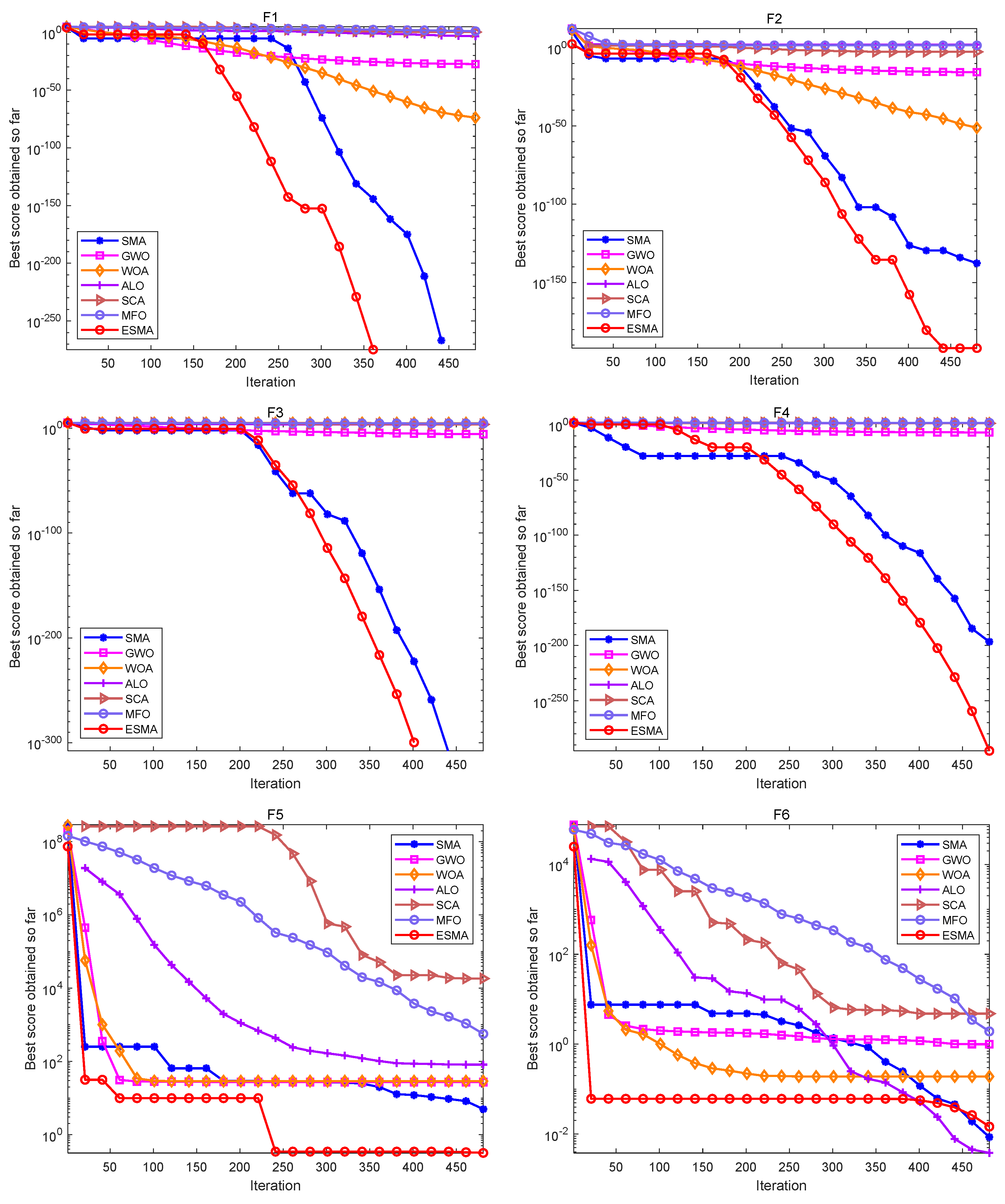
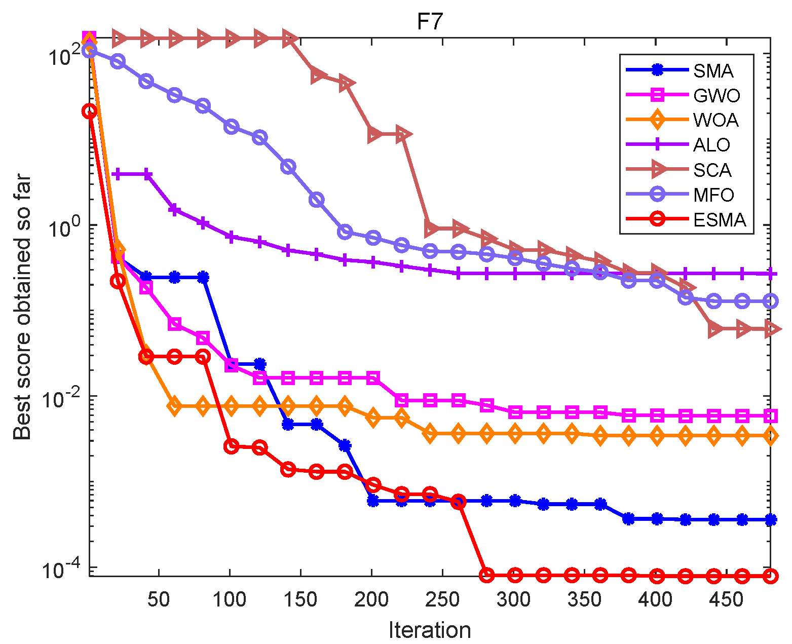
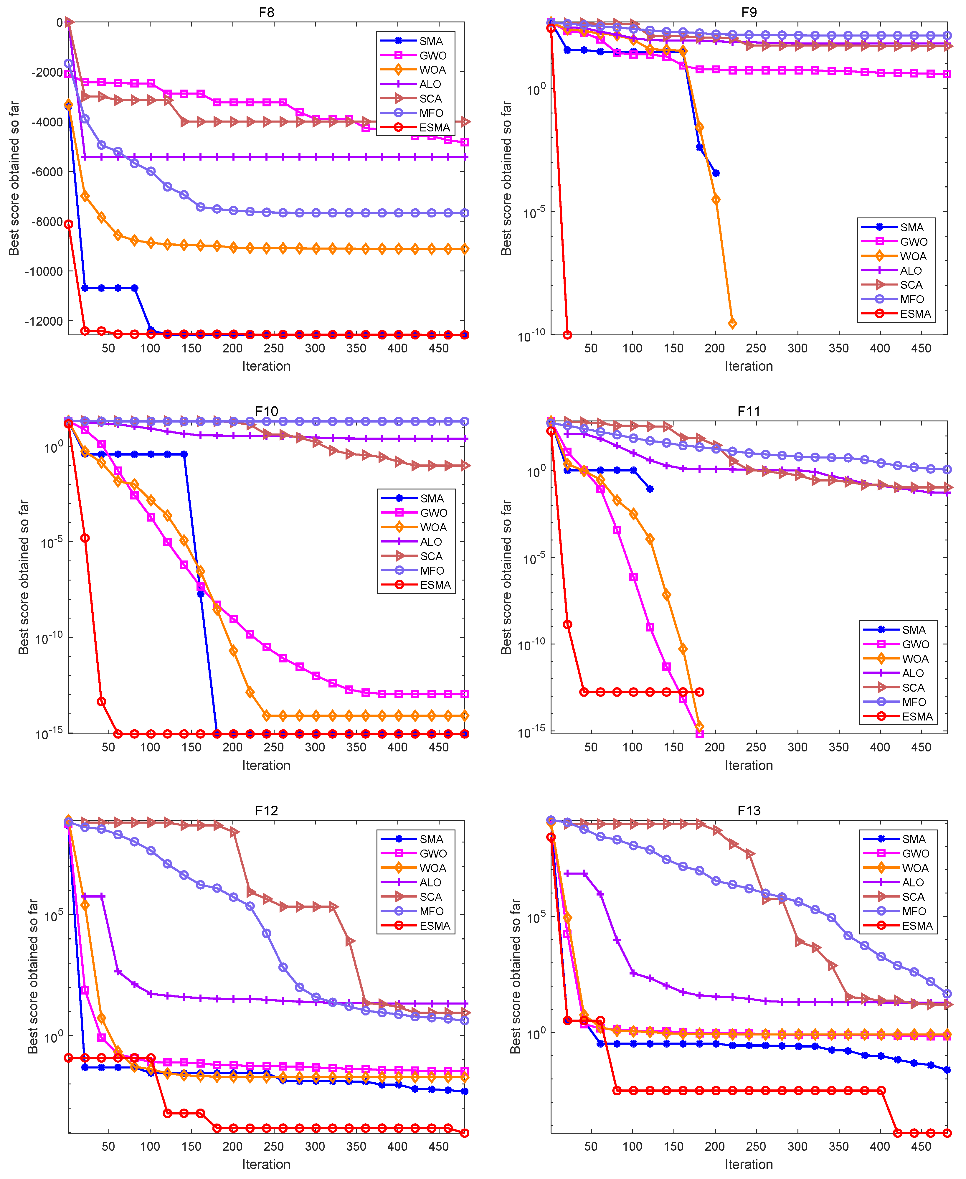
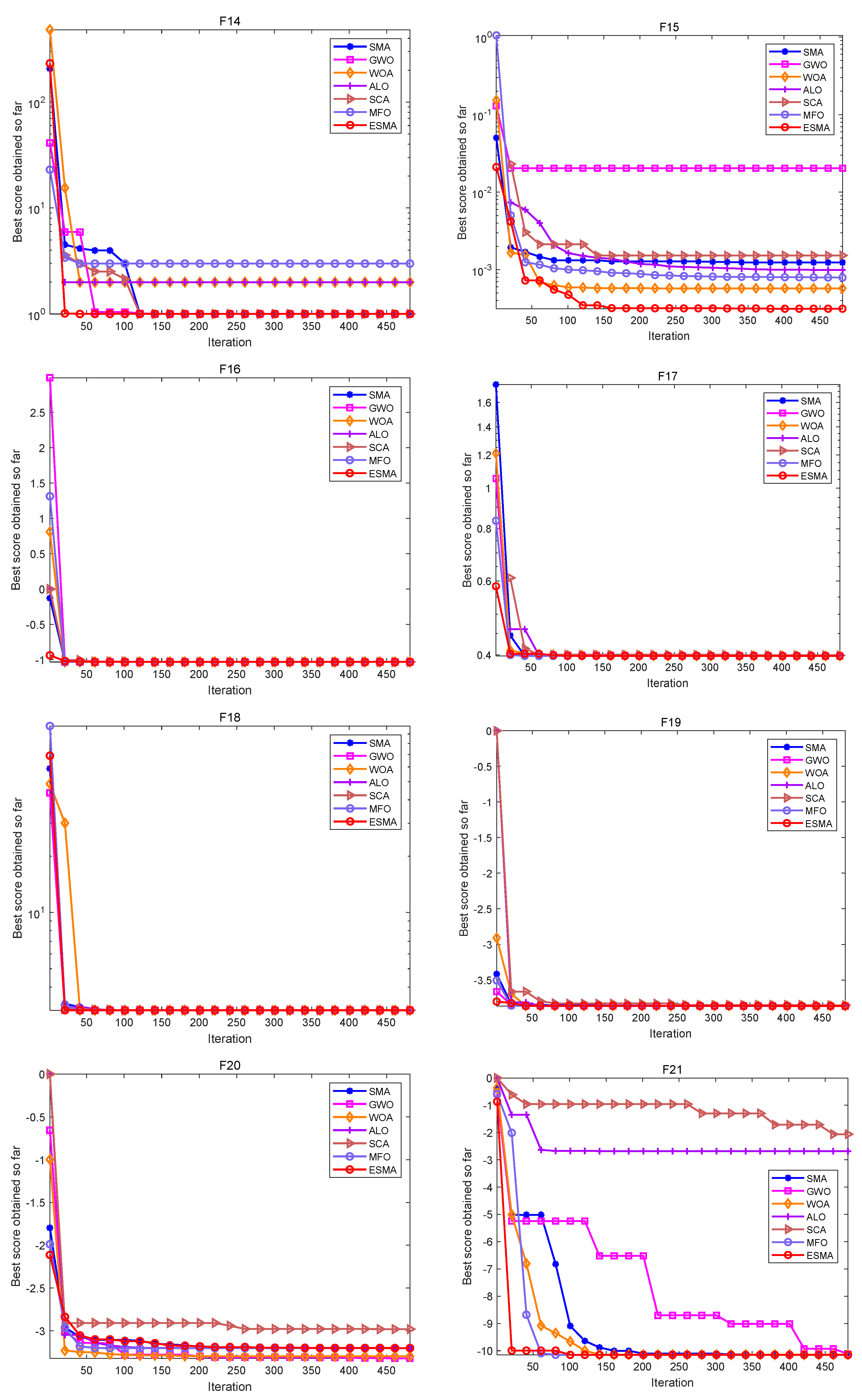
In the simulation experiment of the algorithms, set the population size n = 30, dimension dim = 30, and the maximum number of iterations max_t = 500. In order to eliminate the influence of random factors on the experimental results, and to carry out better statistical analysis on the algorithms, each algorithm runs independently on each benchmark function 20 times, and gives the best value (Best), worst value (Worst), mean value (Mean), standard deviation (Std) and the Rank obtained according to the average value of each algorithm. The specific algorithms comparison results are shown in Table 6 and Figure 1, Figure 2 and Figure 3.
As shown in Table 6, for the unimodal test functions, namely, F1–F7, the ESMA can accurately obtain the optimal value of the test functions on both F1–F4, showing good optimization performance. The ESMA is slightly inferior to ALO on function F6, but obviously superior to it on other unimodal test functions. For the multimodal test functions, namely, F8–F13, the ESMA can also accurately obtain the optimal value of the test functions on F9 and F11, and it is obviously better than other algorithms on other test functions. For the low-dimensional multimodal test functions, the ESMA can also accurately obtain the optimal value of the test functions on F14, F16, and F18, and the optimization results of the seven algorithms on F16 and F18 are basically the same. On function F16–F19, the mean value of the ESMA and MFO algorithm is the same, but the standard deviation of the ESMA is slightly lower than that of the MFO algorithm. The ESMA is obviously better than other algorithms in other low dimensional multimodal test functions. Considering all the test functions, the standard deviation of the ESMA is small, so it is relatively stable on the test functions. According to the final ranking, the ESMA performs well in the 23 benchmark test functions.
Wilcoxon rank sum test, as a nonparametric test, can effectively evaluate the significant differences between the two optimizers. Table 7 shows the values of p obtained by the Wilxocon rank sum test for the other six algorithms under the condition of significance level = 0.05 and taking the ESMA as the benchmark. In order to avoid Type I error, the p-value is corrected using Holm–Bonferroni correction method, and the process is as follows: First, the p-value of six comparison algorithms are sorted from small to large, if the sorting result is assumed to be , if , , , , , , it is considered that there are significant differences between the ESMA and the comparison algorithms. If a p-value is greater than the corresponding value, there is no significant difference between this algorithm corresponding to this p-value and the ESMA, and the subsequent comparison algorithm also has no significant difference from the ESMA whether the p-value is smaller than the corresponding value or not. The bold data in Table 7 are p-value data with no significant difference between the ESMA and its comparison algorithms. Combined with the data in Table 6, p-value are marked accordingly, where “+” means that the comparison algorithm is significantly better than the ESMA, “=“ means that the comparison algorithm has no significant difference with the ESMA, and “-” means that the comparison algorithm is significantly inferior to the ESMA.
From the last line of Table 7, the number of the SMA, GWO, WOA, ALO, SCA, and MFO superior to/similar to/inferior to the ESMA is 0/15/8, 0/2/21, 0/4/19, 4/4/15, 0/0/23, and 4/3/16, this shows that the ESMA is significantly better than comparison algorithm. Therefore, considering Table 6 and Table 7, the ESMA shows good competitiveness.
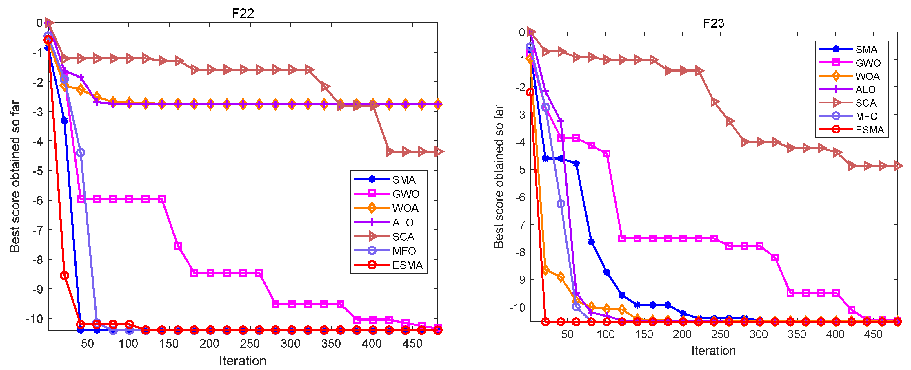
Figure 1, Figure 2 and Figure 3 are convergence curves plotted by the average fitness values obtained by each algorithm running 20 times on the test functions. As shown in Figure 1, for unimodal test functions, the ESMA is significantly better than other comparison algorithms in terms of convergence speed and convergence precision, except for the convergence precision of function F6, which is slightly inferior to the ALO algorithm. As shown in Figure 2, for multimodal test functions, the ESMA is also significantly better than other comparison algorithms in terms of convergence speed and convergence precision, and has good competitiveness. As shown in Figure 3, for the low-dimensional multimodal test functions, in the test function F16–F19, the difference between the seven algorithms is small, and they are basically close to the optimal value of the test function. For function F20, the ESMA is slightly inferior to the WOA and GWO in terms of convergence accuracy, while for other low-dimensional multimodal test functions, the ESMA performs better in terms of convergence speed and accuracy. In general, through the test of convergence curves, the proposed ESMA has obvious improvement in the convergence characteristics on the CEC-2005 benchmark functions.
4. The ESMA for Demand Estimation of Water Resources
4.1. Establishment of Water Resources Demand Estimation Model
In this section, the water resources demand forecasting model of Nanchang City, China, is established. The water resources demand of a city is related to many factors, such as ecological environment and economic development, so it is of great significance to forecast the water resources demand of a city. Table 8 shows the data of the total city water consumption, agricultural water consumption, industrial water consumption, residential water consumption, and ecological water consumption in Nanchang from 2004 to 2019.
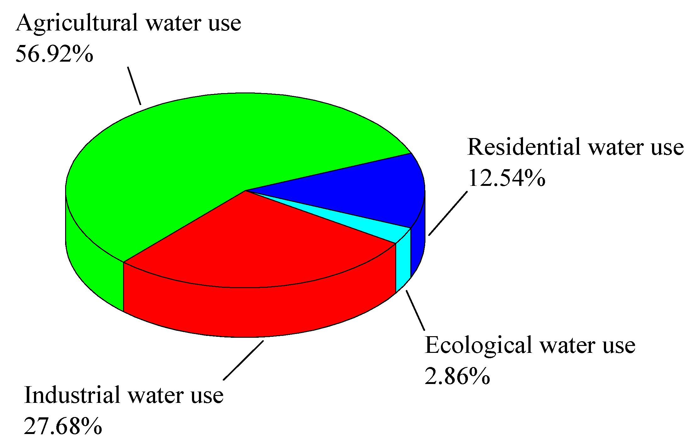
In order to show the relationship between water resources and regional economic development level, water consumption in different areas can be connected with the corresponding economic indicators and population size. For agricultural and industrial water consumption, the water is mainly used for crop irrigation and industrial production, respectively. Therefore, the gross agricultural production, and gross industrial production are appropriate indicators for agricultural and industrial water consumption. Residential water consumption refers to the water that residents need for daily life, including drinking, washing, and bathing, which is closely related to the population size of Nanchang City. However, ecological water consumption is the total amount of water needed to maintain the integrity of an ecosystem, which is not used as social and economic water. This factor is not applicable to explain the relationship between water consumption and the national economy. On the other hand, as shown in Figure 4, ecological water use occupies the smallest proportion of the total water consumption, only 2.86%. Therefore, this paper ignores the ecological water use when establishing the water resources estimation model, and only considers the influence of industrial water use, agricultural water use, and residential water use on the total water consumption.
Table 8 summarizes population size, gross industrial production, and gross agricultural production from 2004 to 2019, which are used to replace industrial water, agricultural water, and residential water.
In view of the relationship between total water consumption and population, gross industrial production, and gross agricultural production, the linear model, logarithmic model, and exponential model for forecasting the water resource of Nanchang City are respectively expressed as,
Linear model:
Logarithmic model:
Exponential model:
In the above model, is the parameter in the model, , , and , respectively represent the population, gross industrial production, and gross agricultural production of Nanchang, and is the water resources demand estimated by the model.
Hybrid model: By combining the above models, this paper obtains a hybrid water resources demand forecasting model based on a linear model, logarithmic model, and exponential model. The hybrid model is established as follows,
where, is the parameter to be estimated. , , and are consistent with Equations (15)–(17).
4.2. Optimization of Water Resources Demand Estimation Model
There are uncertain parameters in the above four water demand estimation models. The selection of parameters is closely related to the accuracy of model forecasting. Therefore, how to determine the parameters in the model is the main issue discussed in this section. The selection of model parameters can be regarded as an optimization problem. In order to evaluate the strengths and weaknesses of parameters in the water resources demand forecasting model, the sum of the squares of errors between the real value and the predicted value is used as the objective function, and its mathematical equation is as follows,
where, X is the parameter in the water resource demand forecasting model, k is the number of years used in the optimization model, is the real total water consumption in the i-th year, and is the estimated total water consumption in the i-th year. The smaller the value of the objective function is, the better the model parameters are, and the closer the predicted value is to the real value. Therefore, the mathematical model of the optimization problem of water demand estimation model can be defined as,
where, X is the D-dimensional decision variable, D is the number of parameters in the estimation model, and are the upper and lower bounds of parameters.
4.3. The ESMA Solves the Parameters of Water Demand Estimation Model
Section 4.2 establishes a specific mathematical model for solving water resources demand parameters. The following shows the specific steps of solving the model with the ESMA.
Step1: Initialize some parameters related to the ESMA, and take Equation (20) as the objective function;
Step2: Initialize the population randomly, and perform the opposition-based learning operation;
Step3: When t < max_t, the fitness value of each individual is calculated, the best and the worst fitness values are updated;
Step4: Update the value of weight W with Equation (6), update the minimum fitness value as the optimal value best_fitness, and record the optimal individual Xb corresponding to the optimal value;
Step5: Update parameters p, vb, and vc for each individual, and update population position according to Equation (8);
Step6: Perform opposition-based learning operation, and then execute elite chaotic searching strategy;
Step7: Let t = t + 1, if t < max_t, returns Step3, otherwise, outputs the optimal value best_fitness and the optimal individual Xb.
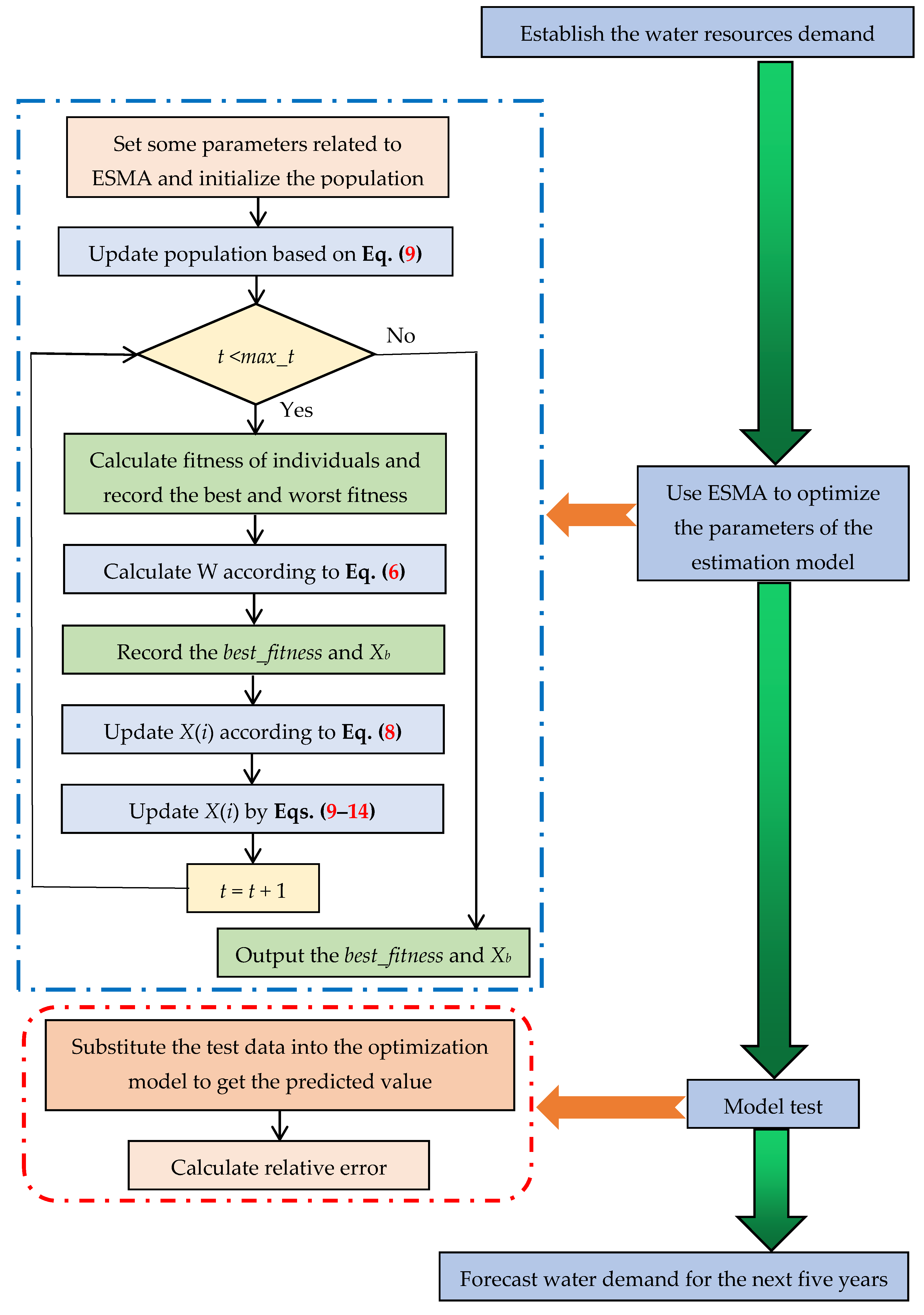
Figure 5 shows the flow chart of the ESMA for solving water resources estimation parameters.
4.4. The Experiment and Analysis of Water Resources Demand Estimation Model
Based on the water resources data of Nanchang City from 2004 to 2019 in Table 9, different optimization algorithms are used to optimize the parameters in different forecasting models, and the performance of different models and algorithms are obtained according to the error analysis between the optimized forecasting values and the real data.
4.4.1. Data Preprocessing
In order to eliminate the influence of magnitude among different data, the data in Table 9 is preprocessed firstly, and the data is normalized as follows,
In the formula, is the normalized data, xij is the j-th index in the i-th year. i = 1, 2, ..., 16 corresponds to 2004–2019, j = 1, 2, 3, 4 corresponds to the total water use, the population, the gross industrial production, and the gross agricultural production, and xjmin and xjmax are the maximum and minimum value of the j-th index, respectively.
4.4.2. Algorithm Parameters Setting
For all algorithms, the population number n is 30, the number of iterations T is 1000, and the dimension D is the number of parameters of the optimized model (Linear model D = 4; Logarithmic model D = 4; Exponential model D = 7; Hybrid model D = 17). To eliminate the influence of random factors, each algorithm is run 20 times independently on different models.
Meanwhile, seven other algorithms are employed to compare with the ESMA in solving the problem of water resources demand estimation. These comparison algorithms are the salp swarm algorithm (SSA) [32], WOA [11], HHO [13], biogeography based optimization (BBO) [33], multi-verse optimizer (MVO) [34], archimedes optimization algorithm (AOA) [35], and SMA [17]. The parameters in these algorithms are set as Table 10 shows.
4.4.3. Performance Evaluation Criteria of the Algorithms
In this paper, the relative error (RE) and mean relative error (MRE) between the real value and the predicted value are used to evaluate the performance of different algorithms in handling different optimization models.
The relative error is calculated by the following formula,
where, and are the real value and estimated value of water resources demand, respectively.
And the calculation formula of mean relative error is as follows,
where, is the real value of water resources demand in the i-th year, is the estimated value of water resources demand in the i-th year, and k is the number of years used in the optimization model.
4.4.4. Result and Analysis
Table 11, Table 12, Table 13 and Table 14 present the average relative error data obtained by the ESMA and seven other optimization algorithms on the four estimation models, including the optimal value, average value, maximum value, and standard deviation after 20 independent runs. The bold data represents the optimal data of all algorithms on the corresponding indexes.
From the perspective of the algorithm, the ESMA performs better on different models. In the linear model (Table 11), the worst value and standard deviation solved by the ESMA are small. In the logarithmic model (Table 12) and exponential model (Table 13), the mean value, maximum value, and standard deviation solved by the ESMA are all small, and the minimum value and mean value solved by the ESMA in the hybrid model (Table 14) are superior to other algorithms. This shows that the ESMA can solve the parameters to minimize the prediction error well in different models. At the same time, the smaller mean value and standard deviation can reflect that the algorithm has good stability when solving the optimization problem and is not easy to be affected by other factors. The worst value and standard deviation of the HHO in the hybrid model (Table 14) are small, indicating that the stability of the algorithm is good, but the results of solving the mean value and the optimal value are not ideal. Overall, the results of the ESMA are better than those of other algorithms.
From the perspective of the forecasting model, the minimum error of the hybrid water demand estimation model in the experimental is 2.2954%, which is better than the error value of other models, indicating that this model can reasonably solve the problem of water resources forecasting, but its stability is slightly weaker than that of logarithmic and exponential models.
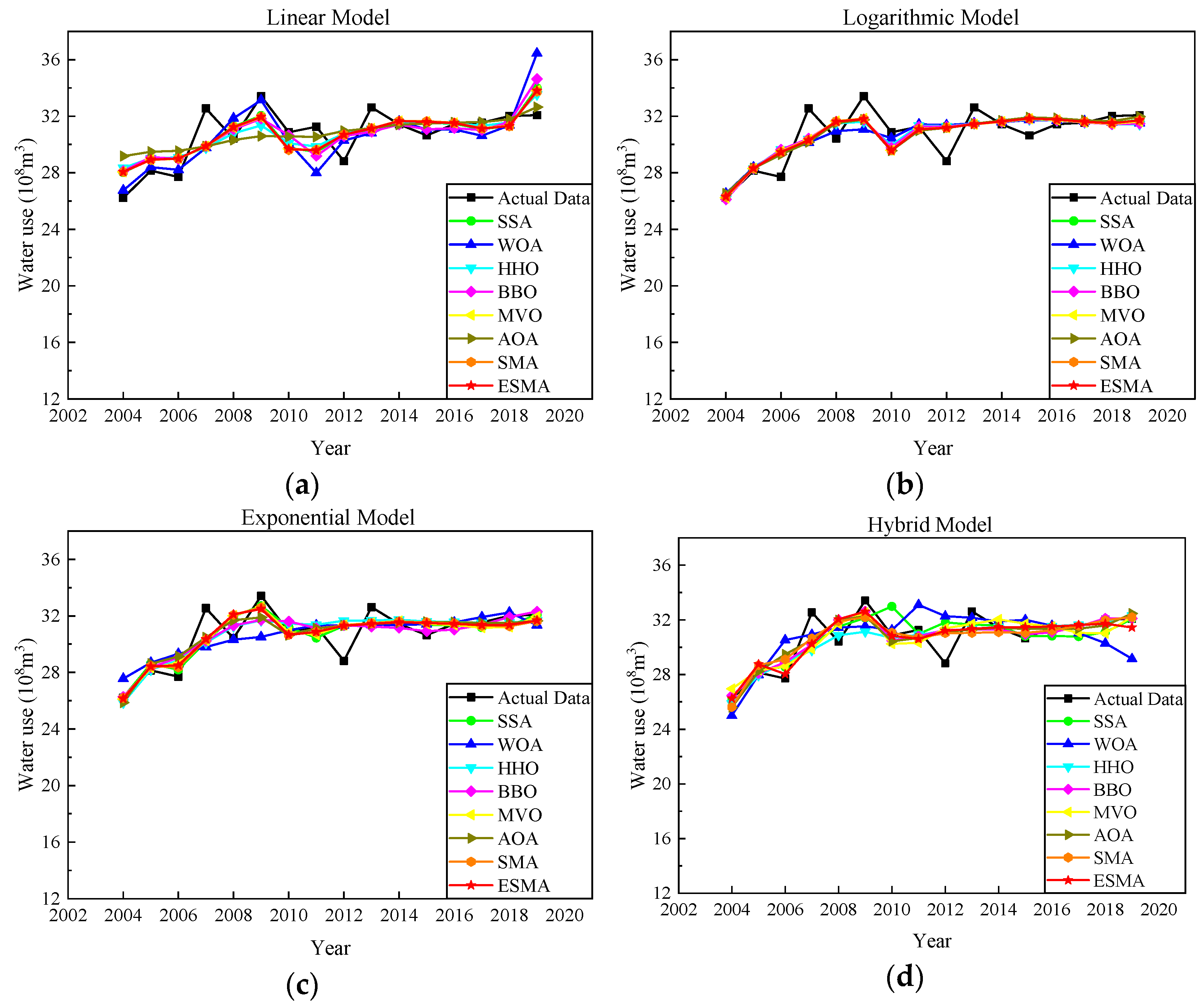
Figure 6 shows the comparison between the forecasting data obtained by substituting the average value of model parameters obtained from 20 runs of different algorithms into the four prediction models and the actual value. The red curve in the figure represents the forecasting data of the ESMA, which is close to the actual data.
4.5. Forecast of Water Resources Demand for 2020–2024
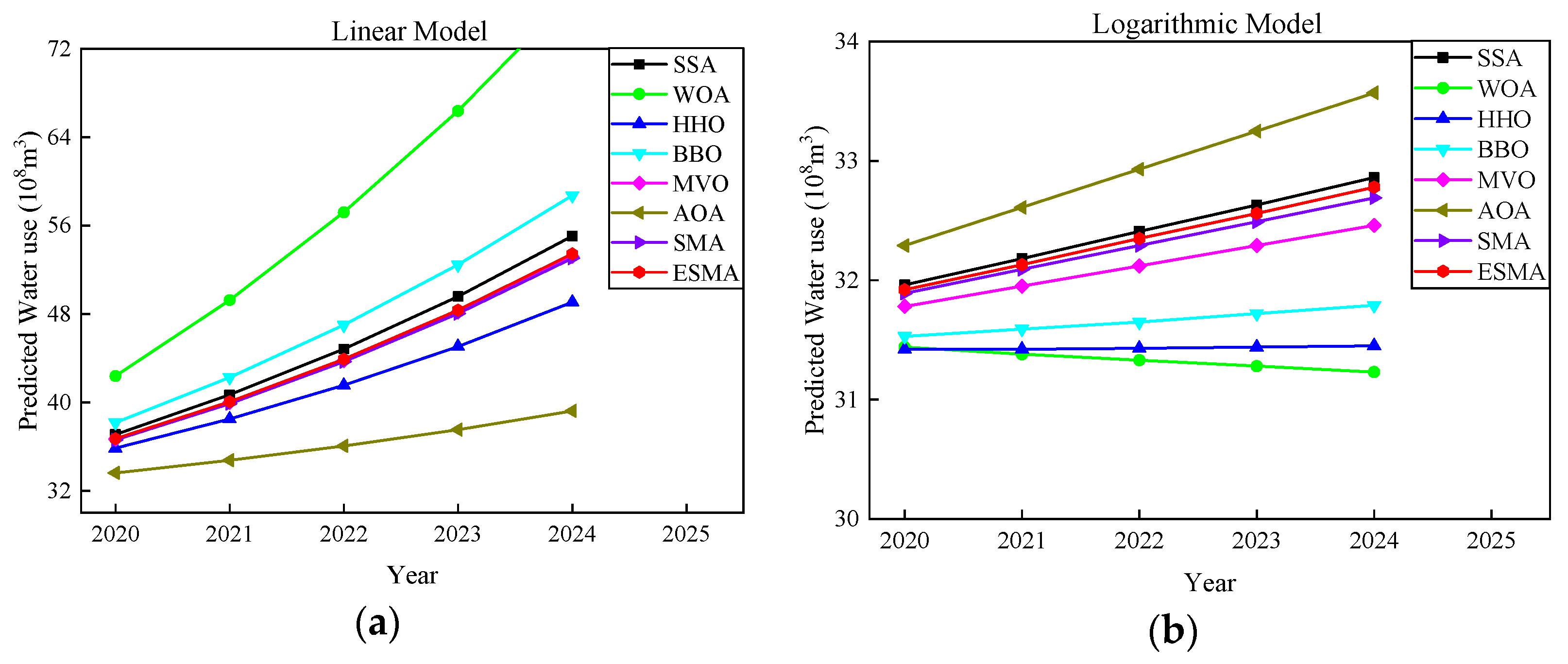
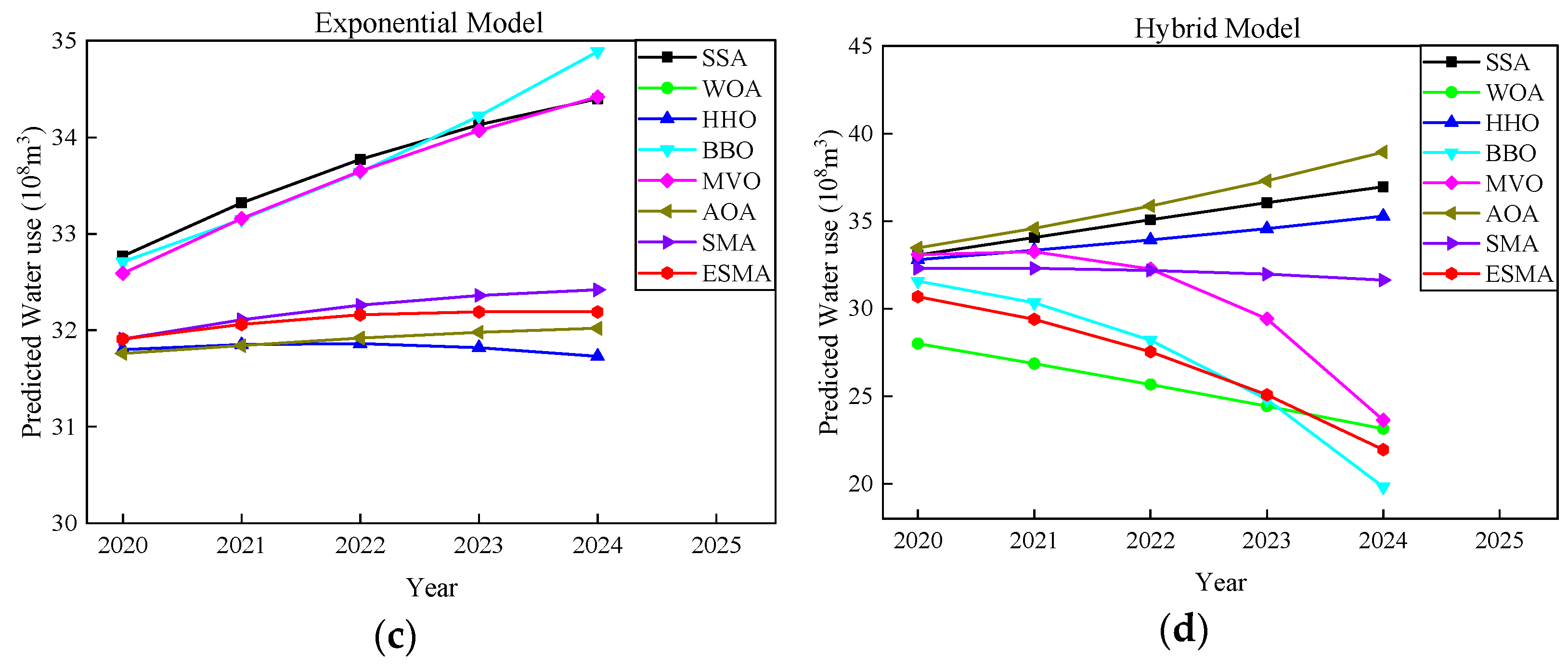
In order to forecast the demand for water resources in Nanchang in 2020–2024, the population, gross industrial production, and gross agricultural production of the above five years are first estimated based on the average annual growth rate. The results are shown in Table 15. Then, by using the parameters of different water demand estimation models obtained by the eight optimization algorithms, the predicted value of water resource demands in 2020–2024 can be obtained. The predicted results are shown in Table 16.
Figure 7 shows the forecast graph of water demand by different algorithms on the four models. Obviously, the prediction curves of the ESMA on each model are located between the results predicted by other algorithms, which may be more in line with the actual use of water resources.
5. Conclusions
In this paper, the ESMA is proposed to estimate the water demand of Nanchang City. In the ESMA, the opposition-based learning strategy is adopted to enhance the diversity of the population and improve the convergence accuracy of the algorithm. The implementation of the elite chaos searching strategy enhances the exploitation ability of the algorithm, which enables the ESMA to better approach the theoretical optimal value of the 23 benchmark functions. According to the relationship between the total water consumption, and the population, the gross industrial production, and the gross agricultural production, four forecasting models of linear, exponential, logarithmic, and hybrid prediction for the water resources in Nanchang City are put forward.
In the experiment, based on the water demand data of Nanchang City from 2004 to 2019, the ESMA is used to optimize the parameters in the estimation models, and the models are tested. The water consumption from 2004 to 2019 is estimated by the ESMA, and the performance of the ESMA is compared with the SMA, SSA, WOA, HHO, BBO, MVO, and AOA. The experimental results show that the ESMA can predict the water consumption with good accuracy on the four models, and it can achieve the highest accuracy in the hybrid estimation model, which is 97.705%. At the end of the experiment, the prediction data of the water demand of Nanchang from 2020 to 2024 by each algorithm are given.
Author Contributions
Conceptualization, K.Y.; Data curation, L.L. and Z.C.; Formal analysis, K.Y., L.L. and Z.C.; Funding acquisition, K.Y.; Investigation, K.Y., L.L. and Z.C.; Methodology, K.Y., L.L. and Z.C.; Resources, K.Y.; Software, L.L. and Z.C.; Supervision, K.Y.; Validation, L.L. and Z.C.; Visualization, Z.C.; Writing—original draft, K.Y., L.L. and Z.C.; Writing—review & editing, K.Y. All authors have read and agreed to the published version of the manuscript.
Funding
This work is supported by National Key R&D Program of China (Grant No. 2019YFD1100905).
Institutional Review Board Statement
Not applicable.
Informed Consent Statement
Not applicable.
Data Availability Statement
All data generated or analysed during this study are included in this published article.
Conflicts of Interest
The authors declare that there is no conflict of interests regarding the publication of this paper.
References
- Davijani, M.H.; Banihabib, M.E.; Anvar, A.N.; Hashemi, S.R. Optimization model for the allocation of water resources based on the maximization of employment in the agriculture and industry sectors. J. Hydrol. 2016, 533, 430–438. [Google Scholar] [CrossRef]
- Arbués, F.; García-Valiñas, M.Á.; Martínez-Espiñeira, R. Estimation of residential water demand: A state-of-the-art review. J. Soc. Econ. 2003, 32, 81–102. [Google Scholar] [CrossRef]
- Hang, L.; Chi, Z.; Dong, M.; Ming, Z. Water demand prediction of Grey Markov model based on GM(1,1). In Proceedings of the 2016 3rd International Conference on Mechatronics and Information Technology, Shenzhen, China, 9–10 April 2016. [Google Scholar]
- Brentan, B.M.; Luvizotto, E., Jr.; Herrera, M.; Lzquierdo, J.; Pérez-García, R. Hybrid regression model for near real-time urban water demand forecasting. J. Comput. Appl. Math. 2017, 309, 532–541. [Google Scholar] [CrossRef]
- Al-Zahrani, M.A.; Abo-Monasar, A. Urban Residential Water Demand Prediction Based on Artificial Neural Networks and Time Series Models. Water Resour. Manag. 2015, 29, 3651–3662. [Google Scholar] [CrossRef]
- Bai, Y.; Wang, P.; Li, C.; Xie, J.J.; Wang, Y. A multi-scale relevance vector regression approach for daily urban water demand forecasting. J. Hydrol. 2014, 517, 236–245. [Google Scholar] [CrossRef]
- Pulido-Calvo, I.; Gutiérrez-Estrada, J.C. Improved irrigation water demand forecasting using a soft-computing hybrid model. Biosyst. Eng. 2009, 102, 202–218. [Google Scholar] [CrossRef]
- Romano, M.; Kapelan, Z. Adaptive water demand forecasting for near real-time management of smart water distribution systems. Environ. Modell. Softw. 2014, 60, 265–276. [Google Scholar] [CrossRef] [Green Version]
- Oliveira, P.J.; Steffen, J.L.; Cheung, P. Parameter estimation of seasonal arima models for water demand forecasting using the harmony search algorithm. Procedia Eng. 2017, 186, 177–185. [Google Scholar] [CrossRef]
- Kennedy, J.; Eberhart, R.C. Particle swarm optimization. In Proceedings of the IEEE International Conference on Neural Networks, Perth, WA, Australia, 27 November–1 December 1995; pp. 1942–1948. [Google Scholar]
- Mirjalili, S.; Lewis, A. The whale optimization algorithm. Adv. Eng. Soft. 2016, 95, 51–67. [Google Scholar] [CrossRef]
- Mirjalili, S.; Mirjalili, S.M.; Lewis, A. Grey wolf optimizer. Adv. Eng. Soft. 2014, 69, 46–61. [Google Scholar] [CrossRef] [Green Version]
- Heidari, A.; Mirjalili, S.; Farris, H.; Aljarah, I.; Mafarja, M.; Chen, H. Harris hawks optimization: Algorithm and applications. Future Gener. Comput. Syst. 2019, 97, 849–872. [Google Scholar] [CrossRef]
- Yang, X.S. Firefly algorithm, stochastic test functions and design optimization. Int. J. Bio Inspir. Comput. 2010, 2, 78–84. [Google Scholar] [CrossRef]
- Zhao, W.G.; Zhang, Z.X.; Wang, L.Y. Manta ray foraging optimization: An effective bio-inspired optimizer for engineering applications. Eng. Appl. Artif. Intell. 2020, 87, 103300. [Google Scholar] [CrossRef]
- Faramarzi, A.; Heidarinejad, M.; Mirjalil, S.; Gandomi, A.H. Marine Predators Algorithm: A nature-inspired metaheuristic. Expert Syst. Appl. 2020, 152, 113377. [Google Scholar] [CrossRef]
- Li, S.M.; Chen, H.L.; Wang, M.J.; Heidari, A.A.; Mirjalili, S. Slime mould algorithm: A new method for stochastic optimization. Future Gener. Comput. Syst. 2020, 111, 300–323. [Google Scholar] [CrossRef]
- Vashishtha, G.; Chauhan, S.; Singh, M.; Kumar, R. Bearing defect identification by swarm decomposition considering permutation entropy measure and opposition-based slime mould algorithm. Measurement 2021, 178, 109389. [Google Scholar] [CrossRef]
- Mostafa, M.; Rezk, H.; Aly, M.; Ahmed, E.M. A new strategy based on slime mould algorithm to extract the optimal model parameters of solar PV panel. Sustain. Energy Techn. 2020, 42, 100849. [Google Scholar] [CrossRef]
- Abdel-Basset, M.; Mohamed, R.; Chakrabortty, R.K.; Ryan, M.J.; Mirjalili, S. An efficient binary slime mould algorithm integrated with a novel attacking-feeding strategy for feature selection. Comput. Ind. Eng. 2021, 153, 107078. [Google Scholar] [CrossRef]
- Kumar, C.; Raj, T.D.; Premkumar, M.; Raj, T.D. A new stochastic slime mould optimization algorithm for the estimation of solar photovoltaic cell parameters. Optik 2020, 223, 165277. [Google Scholar] [CrossRef]
- Rizk-Allah, R.M.; Hassanien, A.E.; Song, D.R. Chaos-opposition-enhanced slime mould algorithm for minimizing the cost of energy for the wind turbines on high-altitude sites. ISA Trans. 2021, in press. [Google Scholar] [CrossRef]
- Abdel-Basset, M.; Chang, V.; Mohamed, R. HSMA_WOA: A hybrid novel Slime mould algorithm with whale optimization algorithm for tackling the image segmentation problem of chest X-ray images. Appl. Soft Comput. 2020, 95, 106642. [Google Scholar] [CrossRef]
- Houssein, E.H.; Mahdy, M.A.; Blondin, M.J.; Shebl, D.; Mohamed, W.M. Hybrid slime mould algorithm with adaptive guided differential evolution algorithm for combinatorial and global optimization problems. Expert Syst. Appl. 2021, 174, 114689. [Google Scholar] [CrossRef]
- Djekidel, R.; Bentouati, B.; Javaid, M.S.; Bouchekara, H.R.E.H.; Bayoumi, A.S.; El-Sehiemy, R.A. Mitigating the effects of magnetic coupling between HV Transmission Line and Metallic Pipeline using Slime Mould Algorithm. J. Magn. Magn. Mater. 2021, 529, 167865. [Google Scholar] [CrossRef]
- El-Fergany, A.A. Parameters identification of PV model using improved slime mould optimizer and Lambert W-function. Energy Rep. 2021, 7, 875–887. [Google Scholar] [CrossRef]
- Tizhoosh, R.H. Opposition-based learning: A new scheme for machine intelligence. In Proceedings of the International Conference on Computational Intelligence for Modelling, Control & Automation and International Conference on Intelligent Agents, Vienna, Austria, 28–30 November 2005; pp. 695–701. [Google Scholar]
- Muthusamy, H.; Ravindran, S.; Yaacob, S.; Polat, K. An improved elephant herding optimization using sine-cosine mechanism and opposition based learning for global optimization problems. Expert Syst. Appl. 2021, 172, 114607. [Google Scholar] [CrossRef]
- Mirjalili, S. The ant lion optimizer. Adv. Eng. Soft. 2015, 83, 80–98. [Google Scholar] [CrossRef]
- Mirjalili, S. SCA: A Sine Cosine Algorithm for solving optimization problems. Knowl. Based Syst. 2016, 96, 120–133. [Google Scholar] [CrossRef]
- Mirjalili, S. Moth-flame optimization algorithm: A novel nature-inspired heuristic paradigm. Knowl. Based Syst. 2015, 89, 228–249. [Google Scholar] [CrossRef]
- Mirjalili, S.; Gandomi, A.H.; Mirjalili, S.Z.; Saremi, S.; Faris, H.; Mirjalili, S.M. Salp swarm algorithm: A bio-inspired optimizer for engineering design problems. Adv. Eng. Soft. 2017, 114, 163–191. [Google Scholar] [CrossRef]
- Xing, B.; Gao, W.J. Biogeography—Based Optimization Algorithm; Springer: Berlin/Heidelberg, Germany, 2014. [Google Scholar]
- Mirjalili, S.; Mirjalili, S.M.; Hatamlou, A. Multi-Verse Optimizer: A nature-inspired algorithm for global optimization. Neural Comput. Appl. 2015, 27, 495–513. [Google Scholar] [CrossRef]
- Hashim, F.A.; Hussain, K.; Houssein, E.H.; Mai, S.M.; Ai-Atabany, W. Archimedes optimization algorithm: A new metaheuristic algorithm for solving optimization problems. Appl. Intell. 2021, 51, 1531–1551. [Google Scholar] [CrossRef]
Figure 1.
Convergence curves of the ESMA and other algorithms on unimodal functions.


Figure 2.
Convergence curves of the ESMA and other algorithms on multimodal functions.

Figure 3.
Convergence curves of the ESMA and other algorithms on fixed-dimensional multimodal functions.
Figure 3.
Convergence curves of the ESMA and other algorithms on fixed-dimensional multimodal functions.


Figure 4.
The distribution of water use in different departments.

Figure 5.
The flow chart of the ESMA for solving water resources estimation parameters.

Figure 6.
Comparison between actual and estimated values for water demand in Nanchang city: (a) Linear model; (b) Logarithmic model; (c) Exponential model; (d) Hybrid model.
Figure 6.
Comparison between actual and estimated values for water demand in Nanchang city: (a) Linear model; (b) Logarithmic model; (c) Exponential model; (d) Hybrid model.

Figure 7.
Comparison for predicting water demand from 2020–2024 based on four models: (a) Linear model; (b) Logarithmic model; (c) Exponential model; (d) Hybrid model.
Figure 7.
Comparison for predicting water demand from 2020–2024 based on four models: (a) Linear model; (b) Logarithmic model; (c) Exponential model; (d) Hybrid model.


Table 1.
Initial parameter settings of all algorithms.
| Algorithm | Parameter Value | Popsize | Iterations of Number |
|---|---|---|---|
| SMA | z = 0.03 | 30 | 500 |
| ESMA | z = 0.03, selected elite proportion pr = 0.1 | 30 | 500 |
| GWO | Component of coefficient vectors: = [2, 0] | 30 | 500 |
| WOA | value of coefficient vectors : = [2, 0] | 30 | 500 |
| ALO | NA | 30 | 500 |
| SCA | The value of constant = 2 | 30 | 500 |
| MFO | b = 1 | 30 | 500 |
Table 2.
Details Settings.
| Classification | Name | Detailed Settings |
|---|---|---|
| Hardware | CPU | Intel(R) Core(TM) i5-8625U |
| Frequency | 1.60 GHz 1.80 GHz | |
| RAM | 8.00 GB | |
| Hard drive | 512 GB | |
| Software | Operating system | Windows 10 |
| Language | MATLAB R2018a |
Table 3.
Unimodal test functions.
| Function | D | Range | fopt |
|---|---|---|---|
| 30 | [−100, 100]n | 0 | |
| 30 | [−10, 10]n | 0 | |
| 30 | [−100, 100]n | 0 | |
| 30 | [−100, 100]n | 0 | |
| 30 | [−30, 30]n | 0 | |
| 30 | [−100, 100]n | 0 | |
| 30 | [−1.28, 1.28]n | 0 |
Table 4.
Multimodal test functions.
| Function | D | Range | fopt |
|---|---|---|---|
| 30 | [−500, 500]n | −12,569.5 | |
| 30 | [−5.12, 5.12]n | 0 | |
| 30 | [−32, 32]n | 0 | |
| 30 | [−600, 600]n | 0 | |
| 30 | [−50, 50]n | 0 | |
| 30 | [−50, 50]n | 0 |
Table 5.
Fixed-dimensional multimodal test functions.
| Function | D | Range | fopt |
|---|---|---|---|
| 2 | [−65.536, 65.536]n | 0.998 | |
| 4 | [−5, 5]n | 3.075 × 10⁻⁴ | |
| 2 | [−5, 5]n | −1.0316 | |
| 2 | [−5, 5]n | 0.398 | |
| 2 | [−2, 2]n | 3 | |
| 3 | [0, 1]n | −3.86 | |
| 6 | [0, 1]n | −3.322 | |
| 4 | [0, 10]n | −10.1532 | |
| 4 | [0, 10]n | −10.4028 | |
| 4 | [0, 10]n | −10.5363 |
Table 6.
Results of the ESMA and other optimization algorithms.
| Algorithms | ||||||||
|---|---|---|---|---|---|---|---|---|
| GWO | WOA | ALO | SCA | MFO | SMA | ESMA | ||
| F1 | Best | 4.31E-29 | 7.16E-82 | 2.00E-4 | 4.41E-3 | 7.01E-1 | 0 | 0 |
| Worst | 6.38E-27 | 7.28E-75 | 5.01E-3 | 4.52E+1 | 2.00E+4 | 0 | 0 | |
| Mean | 1.48E-27 | 9.44E-76 | 1.57E-3 | 1.09E+1 | 3.03E+3 | 0 | 0 | |
| Std | 2.01E-27 | 1.84E-75 | 1.21E-3 | 1.32E+1 | 5.70E+3 | 0 | 0 | |
| Rank | 3 | 2 | 4 | 5 | 6 | 1 | 1 | |
| F2 | Best | 3.37E-17 | 2.71E-55 | 2.3137 | 7.20E-6 | 4.07E-1 | 1.54E-284 | 0 |
| Worst | 4.36E-16 | 3.54E-50 | 1.20E+2 | 6.19E-2 | 8.00E+1 | 3.58E-151 | 0 | |
| Mean | 1.31E-16 | 1.87E-51 | 4.73E+1 | 1.23E-2 | 3.04E+1 | 1.79E-152 | 0 | |
| Std | 1.09E-16 | 7.88E-51 | 4.72E+1 | 1.78E-2 | 2.44E+1 | 8.04E-152 | 0 | |
| Rank | 4 | 3 | 7 | 5 | 6 | 2 | 1 | |
| F3 | Best | 2.84E-9 | 1.49E+4 | 1.22E+3 | 2.74E+3 | 1.72E+3 | 0 | 0 |
| Worst | 5.78E-4 | 5.90E+4 | 9.89E+3 | 2.28E+4 | 5.39E+4 | 6.47E-295 | 0 | |
| Mean | 3.37E-5 | 3.75E+4 | 4.12E+3 | 9.45E+3 | 2.08E+4 | 3.24E-296 | 0 | |
| Std | 1.28E-4 | 1.07E+4 | 2.03E+3 | 5.15E+3 | 1.25E+4 | 0 | 0 | |
| Rank | 3 | 7 | 4 | 5 | 6 | 2 | 1 | |
| F4 | Best | 9.21E-8 | 1.6832 | 7.3298 | 1.99E+1 | 5.56E+1 | 3.82E-288 | 0 |
| Worst | 2.10E-6 | 8.93E+1 | 2.71E+1 | 5.30E+1 | 8.48E+1 | 4.17E-156 | 0 | |
| Mean | 6.73E-7 | 5.18E+1 | 1.68E+1 | 3.74E+1 | 6.76E+1 | 2.09E-157 | 0 | |
| Std | 5.89E-7 | 2.81E+1 | 5.1065 | 9.5060 | 8.9481 | 9.33E-157 | 0 | |
| Rank | 3 | 6 | 4 | 5 | 7 | 2 | 1 | |
| F5 | Best | 2.61E+1 | 2.77E+1 | 2.70E+1 | 1.00E+2 | 2.36E+1 | 4.30E-1 | 2.48E-2 |
| Worst | 2.87E+1 | 2.88E+1 | 2.05E+3 | 1.10E+5 | 8.00E+7 | 2.83E+1 | 6.2473 | |
| Mean | 2.73E+1 | 2.82E+1 | 3.24E+2 | 1.69E+4 | 7.80E+6 | 8.8490 | 1.0764 | |
| Std | 8.32E-1 | 1.61E-1 | 2.99E+5 | 7.23E+8 | 5.75E+14 | 1.30E+2 | 2.0468 | |
| Rank | 3 | 4 | 5 | 6 | 7 | 2 | 1 | |
| F6 | Best | 8.26E-5 | 1.19E-1 | 2.68E-4 | 4.9784 | 3.56E-1 | 1.64E-3 | 3.53E-4 |
| Worst | 1.5139 | 1.0976 | 4.22E-3 | 1.68E+2 | 1.01E+4 | 2.08E-2 | 1.01E-2 | |
| Mean | 6.72E-1 | 3.68E-1 | 1.10E-3 | 1.96E+1 | 1.00E+3 | 6.67E-3 | 4.01E-3 | |
| Std | 1.44E-1 | 6.18E-2 | 1.45E-6 | 1.32E+3 | 9.47E+6 | 1.59E-5 | 6.64E-6 | |
| Rank | 5 | 4 | 1 | 6 | 7 | 3 | 2 | |
| F7 | Best | 8.91E-4 | 2.37E-4 | 1.56E-1 | 1.36E-2 | 9.39E-2 | 1.01E-05 | 1.95E-6 |
| Worst | 6.99E-3 | 4.02E-3 | 4.93E-1 | 1.8531 | 2.8949 | 6.07E-4 | 1.86E-4 | |
| Mean | 2.56E-3 | 1.54E-3 | 2.79E-1 | 1.98E-1 | 7.07E-1 | 2.23E-4 | 7.38E-5 | |
| Std | 1.34E-3 | 1.14E-3 | 8.70E-2 | 3.97E-1 | 9.82E-1 | 1.46E-4 | 5.19E-5 | |
| Rank | 4 | 3 | 6 | 5 | 7 | 2 | 1 | |
| F8 | Best | −7729.0907 | −12568.933 | −7095.6123 | −4391.8124 | −9972.9113 | −12,569.38 | −12,569.49 |
| Worst | −3476.3214 | −8256.6973 | −5417.6748 | −3425.6876 | −7105.0606 | −12,568.52 | −12,568.31 | |
| Mean | −5941.1712 | −10,238.026 | −5556.2584 | −3851.2001 | −8482.0979 | −12,569.01 | −12,569.11 | |
| Std | 1.07E+6 | 2.91E+6 | 1.37E+5 | 8.53E+4 | 5.48E+5 | 5.59E-2 | 1.38E-1 | |
| Rank | 5 | 3 | 6 | 7 | 4 | 2 | 1 | |
| F9 | Best | 5.68E-14 | 0 | 4.38E+1 | 4.51E-1 | 1.04E+2 | 0 | 0 |
| Worst | 1.44E+1 | 0 | 1.17E+2 | 1.06E+1 | 2.52E+2 | 0 | 0 | |
| Mean | 3.6616 | 0 | 7.91E+1 | 4.59E+1 | 1.62E+2 | 0 | 0 | |
| Std | 4.1227 | 0 | 1.84E+1 | 2.84E+1 | 3.33E+1 | 0 | 0 | |
| Rank | 2 | 1 | 4 | 3 | 5 | 1 | 1 | |
| F10 | Best | 7.55E-14 | 8.88E-16 | 1.7783 | 1.41E-2 | 1.3811 | 8.88E-16 | 8.88E-16 |
| Worst | 1.22E-13 | 7.99E-15 | 9.7666 | 2.04E+1 | 2.00E+1 | 8.88E-16 | 8.88E-16 | |
| Mean | 9.93E-14 | 3.91E-15 | 4.8695 | 1.52E+1 | 1.38E+1 | 8.88E-16 | 8.88E-16 | |
| Std | 1.33E-14 | 3.11E-15 | 2.5083 | 8.5952 | 7.7738 | 0 | 0 | |
| Rank | 3 | 2 | 4 | 6 | 5 | 1 | 1 | |
| F11 | Best | 0 | 0 | 3.55E-3 | 4.36E-1 | 6.15E-1 | 0 | 0 |
| Worst | 4.11E-2 | 1.10E-1 | 1.27E-1 | 1.3327 | 1.81E+2 | 0 | 0 | |
| Mean | 9.28E-3 | 7.82E-3 | 5.47E-2 | 8.52E-1 | 1.90E+1 | 0 | 0 | |
| Std | 1.33E-2 | 2.62E-2 | 2.87E-2 | 2.60E-1 | 4.71E+1 | 0 | 0 | |
| Rank | 3 | 2 | 4 | 5 | 6 | 1 | 1 | |
| F12 | Best | 1.93E-2 | 8.79E-3 | 7.8128 | 1.2833 | 3.4831 | 4.07E-5 | 1.38E-6 |
| Worst | 1.05E-1 | 4.51E-2 | 3.69E+1 | 1.28E+6 | 2.60E+1 | 1.51E-2 | 9.67E-3 | |
| Mean | 4.25E-2 | 2.13E-2 | 1.56E+1 | 6.44E+4 | 1.00E+1 | 4.91E-3 | 1.29E-3 | |
| Std | 5.75E-4 | 1.18E-4 | 5.44E+1 | 8.25E+10 | 5.31E+1 | 2.23E-5 | 5.61E-6 | |
| Rank | 4 | 3 | 6 | 7 | 5 | 2 | 1 | |
| F13 | Best | 4.46E-1 | 5.88E-2 | 8.49E-2 | 3.0307 | 9.4540 | 4.91E-4 | 2.30E-5 |
| Worst | 1.1132 | 1.1252 | 5.44E+1 | 2.25E+5 | 3.62E+2 | 7.06E-2 | 1.41E-2 | |
| Mean | 7.66E-1 | 4.68E-1 | 2.29E+1 | 1.24E+4 | 4.13E+1 | 1.14E-2 | 3.79E-3 | |
| Std | 3.57E-2 | 8.03E-2 | 3.64E+2 | 2.50E+9 | 5.83E+3 | 2.64E-4 | 1.41E-5 | |
| Rank | 4 | 3 | 5 | 7 | 6 | 2 | 1 | |
| F14 | Best | 0.998 | 0.998 | 0.998 | 0.998 | 0.998 | 0.998 | 0.998 |
| Worst | 12.6705 | 10.7632 | 6.9033 | 10.7632 | 7.874 | 0.998 | 0.998 | |
| Mean | 5.3046 | 3.7499 | 2.7291 | 2.0828 | 3.1201 | 0.998 | 0.998 | |
| Std | 1.95E+1 | 1.11E+1 | 3.0575 | 5.0233 | 5.3292 | 7.86E-24 | 3.30E-25 | |
| Rank | 7 | 6 | 4 | 3 | 5 | 2 | 1 | |
| F15 | Best | 3.075E-4 | 3.078E-4 | 6.404E-4 | 4.884E-4 | 7.295E-4 | 3.075E-4 | 3.077E-4 |
| Worst | 2.036E-2 | 2.194E-3 | 2.036E-2 | 1.535E-3 | 1.655E-3 | 1.227E-3 | 1.231E-3 | |
| Mean | 2.51E-3 | 8.72E-4 | 1.94E-3 | 9.78E-4 | 1.02E-3 | 5.93E-4 | 5.29E-4 | |
| Std | 3.74E-5 | 3.46E-7 | 1.89E-5 | 1.27E-7 | 1.32E-7 | 1.25E-7 | 7.58E-8 | |
| Rank | 7 | 3 | 6 | 4 | 5 | 2 | 1 | |
| F16 | Best | −1.0316 | −1.0316 | −1.0316 | −1.0316 | −1.0316 | −1.0316 | −1.0316 |
| Worst | −1.0316 | −1.0316 | −1.0316 | −1.0316 | −1.0316 | −1.0316 | −1.0316 | |
| Mean | −1.0316 | −1.0316 | −1.0316 | −1.0316 | −1.0316 | −1.0316 | −1.0316 | |
| Std | 5.53E-16 | 5.53E-19 | 5.94E-27 | 2.37E-9 | 5.19E-32 | 1.25E-18 | 3.97E-19 | |
| Rank | 6 | 4 | 2 | 7 | 1 | 5 | 3 | |
| F17 | Best | 0.39789 | 0.39789 | 0.39789 | 0.39789 | 0.39789 | 0.39789 | 0.39789 |
| Worst | 0.39791 | 0.39792 | 0.39789 | 0.40907 | 0.39789 | 0.39789 | 0.39789 | |
| Mean | 0.39789 | 0.39789 | 0.39789 | 0.40037 | 0.39789 | 0.39789 | 0.39789 | |
| Std | 2.62E-11 | 1.00E-10 | 1.17E-26 | 1.11E-5 | 0 | 9.22E-16 | 5.23E-16 | |
| Rank | 5 | 6 | 2 | 7 | 1 | 4 | 3 | |
| F18 | Best | 3 | 3 | 3 | 3 | 3 | 3 | 3 |
| Worst | 3 | 3.0006 | 3 | 3.0004 | 3 | 3 | 3 | |
| Mean | 3 | 3.0001 | 3 | 3.0001 | 3 | 3 | 3 | |
| Std | 1.66E-9 | 2.04E-8 | 6.35E-26 | 1.62E-8 | 7.71E-30 | 1.16E-20 | 1.84E-21 | |
| Rank | 5 | 7 | 4 | 6 | 1 | 3 | 2 | |
| F19 | Best | −3.8628 | −3.8626 | −3.8628 | −3.8549 | −3.8628 | −3.8628 | −3.8628 |
| Worst | −3.8549 | −3.8215 | −3.8628 | −3.8518 | −3.8628 | −3.8628 | −3.8628 | |
| Mean | −3.8611 | −3.852 | −3.8628 | −3.854 | −3.8628 | −3.8628 | −3.8628 | |
| Std | 7.17E-6 | 1.70E-4 | 3.18E-26 | 1.08E-6 | 5.19E-30 | 2.43E-13 | 6.37E-15 | |
| Rank | 5 | 7 | 2 | 6 | 1 | 4 | 3 | |
| F20 | Best | −3.322 | −3.3216 | −3.322 | −3.1454 | −3.322 | −3.322 | −3.322 |
| Worst | −3.1365 | −2.4512 | −3.2018 | −1.9187 | −3.1327 | −3.1974 | −3.1997 | |
| Mean | −3.2502 | −3.1889 | −3.2683 | −2.9488 | −3.2347 | −3.2559 | −3.2142 | |
| Std | 5.84E-3 | 4.05E-2 | 3.70E-3 | 7.15E-2 | 3.68E-3 | 3.76E-3 | 1.36E-3 | |
| Rank | 3 | 6 | 1 | 7 | 5 | 2 | 4 | |
| F21 | Best | −10.1528 | −10.1502 | −10.1532 | −7.7535 | −10.1532 | −10.1532 | −10.1532 |
| Worst | −2.6826 | −2.6271 | −2.6305 | −0.4982 | −2.6305 | −10.152 | −10.1521 | |
| Mean | −7.632 | −7.4809 | −6.3745 | −3.155 | −5.1376 | −10.1527 | −10.1529 | |
| Std | 8.6401 | 9.6374 | 1.09E+1 | 4.1255 | 9.8474 | 1.17E-7 | 1.30E-7 | |
| Rank | 3 | 4 | 5 | 7 | 6 | 2 | 1 | |
| F22 | Best | −10.4028 | −10.4016 | −10.4029 | −6.555 | −10.4029 | −10.4029 | −10.4029 |
| Worst | −10.3969 | -3.7181 | −1.8376 | −0.5239 | −2.7519 | −10.402 | −10.4017 | |
| Mean | −10.4012 | −8.197 | −5.9837 | −3.1307 | −7.5086 | −10.4025 | −10.4026 | |
| Std | 1.73E-6 | 7.6414 | 1.17E+1 | 3.37 | 1.35E+1 | 6.59E-8 | 9.85E-8 | |
| Rank | 3 | 4 | 6 | 7 | 5 | 2 | 1 | |
| F23 | Best | −10.5363 | −10.5357 | −10.5364 | −6.7648 | −10.5364 | −10.5364 | −10.5364 |
| Worst | −2.4217 | −2.4173 | −1.6766 | −0.94237 | −2.8711 | −10.5354 | −10.5351 | |
| Mean | −9.8612 | −7.3348 | −7.2174 | −3.6007 | −8.1616 | −10.5360 | −10.5361 | |
| Std | 4.4991 | 8.9562 | 1.47E+1 | 3.3493 | 1.12E+1 | 9.72E-8 | 8.31E-8 | |
| Rank | 3 | 5 | 6 | 7 | 4 | 2 | 1 | |
| Mean Rank | 4.0435 | 4.1304 | 4.2609 | 5.7826 | 4.8261 | 2.2174 | 1.4783 | |
| Result | 3 | 4 | 5 | 7 | 6 | 2 | 1 | |
Table 7.
The p-value of the Wilcoxon rank sum test, based on the ESMA.
| Function | ESMA vs. SMA | ESMA vs. GWO | ESMA vs. WOA | ESMA vs. ALO | ESMA vs. SCA | ESMA vs. MFO | ||||||
|---|---|---|---|---|---|---|---|---|---|---|---|---|
| F1 | 3.42E-1 | = | 8.01E-9 | - | 8.01E-9 | - | 8.01E-9 | - | 8.01E-9 | - | 8.01E-9 | - |
| F2 | 8.01E-9 | - | 8.01E-9 | - | 8.01E-9 | - | 8.01E-9 | - | 8.01E-9 | - | 8.01E-9 | - |
| F3 | 1.98E-2 | - | 8.01E-9 | - | 8.01E-9 | - | 8.01E-9 | - | 8.01E-9 | - | 8.01E-9 | - |
| F4 | 8.01E-9 | - | 8.01E-9 | - | 8.01E-9 | - | 8.01E-9 | - | 8.01E-9 | - | 8.01E-9 | - |
| F5 | 4.16E-4 | - | 6.80E-8 | - | 6.80E-8 | - | 6.80E-8 | - | 6.80E-8 | - | 6.80E-8 | - |
| F6 | 8.35E-3 | - | 1.20E-6 | - | 6.80E-8 | - | 5.90E-5 | - | 6.80E-8 | - | 6.80E-8 | - |
| F7 | 1.61E-4 | - | 6.80E-8 | - | 6.80E-8 | - | 6.80E-8 | - | 6.80E-8 | - | 6.80E-8 | - |
| F8 | 1.48E-1 | = | 6.80E-8 | - | 1.66E-7 | - | 4.95E-8 | - | 6.80E-8 | - | 6.80E-8 | - |
| F9 | NaN | = | 7.93E-9 | - | NaN | = | 8.01E-9 | - | 8.01E-9 | - | 8.01E-9 | - |
| F10 | NaN | = | 7.68E-9 | - | 1.57E-4 | - | 8.01E-9 | - | 8.01E-9 | - | 8.01E-9 | - |
| F11 | NaN | = | 2.09E-3 | - | 1.63E-1 | = | 8.01E-9 | - | 8.01E-9 | - | 8.01E-9 | - |
| F12 | 6.22E-4 | - | 6.80E-8 | - | 9.17E-8 | - | 6.80E-8 | - | 6.80E-8 | - | 6.80E-8 | - |
| F13 | 4.39E-2 | - | 6.80E-8 | - | 6.80E-8 | - | 6.80E-8 | - | 6.80E-8 | - | 6.80E-8 | - |
| F14 | 9.25E-1 | = | 6.80E-8 | - | 6.80E-8 | - | 3.13E-2 | = | 6.80E-8 | - | 1.06E-1 | = |
| F15 | 9.46E-1 | = | 8.18E-1 | = | 1.44E-2 | - | 2.30E-5 | - | 4.68E-5 | - | 3.71E-5 | - |
| F16 | 6.75E-1 | = | 1.06E-7 | - | 9.89E-1 | = | 6.80E-8 | + | 6.80E-8 | - | 8.01E-9 | + |
| F17 | 9.68E-1 | = | 5.23E-7 | - | 8.35E-3 | - | 6.79E-8 | + | 6.80E-8 | - | 8.01E-9 | + |
| F18 | 1.48E-1 | = | 6.80E-8 | - | 6.80E-8 | - | 9.13E-7 | - | 6.80E-8 | - | 5.71E-8 | + |
| F19 | 1.40E-1 | = | 6.80E-8 | - | 6.80E-8 | - | 6.80E-8 | + | 6.80E-8 | - | 8.01E-9 | + |
| F20 | 3.15E-2 | = | 5.61E-1 | = | 5.98E-1 | = | 6.56E-3 | + | 6.80E-8 | - | 1.29E-3 | - |
| F21 | 8.10E-2 | = | 7.95E-7 | - | 6.80E-8 | - | 2.85E-1 | = | 6.80E-8 | - | 6.93E-3 | - |
| F22 | 2.29E-1 | = | 1.10E-5 | - | 6.80E-8 | - | 1.08E-1 | = | 6.80E-8 | - | 2.83E-1 | = |
| F23 | 2.50E-1 | = | 5.87E-6 | - | 9.17E-8 | - | 5.98E-1 | = | 6.80E-8 | - | 1.04E-1 | = |
| +/=/- | 0/15/8 | 0/2/21 | 0/4/19 | 4/4/15 | 0/0/23 | 4/3/16 | ||||||
Table 8.
Historical water use in Nanchang city from 2004 to 2019.
| Year | Total Water Use (108 m3) | Industrial Water Use (108 m3) | Agricultural Water Use (108 m3) | Residential Water Use (108 m3) | Ecological Water Use (108 m3) |
|---|---|---|---|---|---|
| 2004 | 26.22 | 8.72 | 14.47 | 2.75 | 0.28 |
| 2005 | 28.14 | 8.30 | 16.92 | 2.60 | 0.32 |
| 2006 | 27.71 | 8.11 | 16.73 | 2.52 | 0.35 |
| 2007 | 32.55 | 7.51 | 21.27 | 2.92 | 0.85 |
| 2008 | 30.42 | 6.90 | 19.73 | 2.94 | 0.85 |
| 2009 | 33.42 | 6.57 | 20.15 | 3.21 | 3.49 |
| 2010 | 30.87 | 7.51 | 17.37 | 3.49 | 2.50 |
| 2011 | 31.26 | 8.97 | 17.70 | 4.03 | 0.56 |
| 2012 | 28.82 | 9.20 | 14.68 | 4.36 | 0.58 |
| 2013 | 32.62 | 9.35 | 18.23 | 4.45 | 0.59 |
| 2014 | 31.42 | 8.92 | 17.35 | 4.54 | 0.61 |
| 2015 | 30.64 | 9.17 | 16.21 | 4.64 | 0.62 |
| 2016 | 31.44 | 9.21 | 16.9 | 4.7 | 0.53 |
| 2017 | 31.54 | 9.28 | 16.84 | 4.78 | 0.64 |
| 2018 | 32.02 | 9.13 | 17.45 | 4.8 | 0.64 |
| 2019 | 32.08 | 9.09 | 17.51 | 4.83 | 0.65 |
| Total | 491.17 | 135.94 (27.68%) | 279.51 (56.92%) | 61.56 (12.54%) | 14.06 (2.86%) |
Table 9.
The total water, population, gross industrial production, and gross agricultural production in Nanchang city from 2004 to 2019.
Table 9.
The total water, population, gross industrial production, and gross agricultural production in Nanchang city from 2004 to 2019.
| Year | Total Water Use (108 m3) | Industrial Water Use (108 m3) | Agricultural Water Use (108 m3) | Residential Water Use (108 m3) | Ecological Water Use (108 m3) |
|---|---|---|---|---|---|
| 2004 | 26.22 | 8.72 | 14.47 | 2.75 | 0.28 |
| 2005 | 28.14 | 8.30 | 16.92 | 2.60 | 0.32 |
| 2006 | 27.71 | 8.11 | 16.73 | 2.52 | 0.35 |
| 2007 | 32.55 | 7.51 | 21.27 | 2.92 | 0.85 |
| 2008 | 30.42 | 6.90 | 19.73 | 2.94 | 0.85 |
| 2009 | 33.42 | 6.57 | 20.15 | 3.21 | 3.49 |
| 2010 | 30.87 | 7.51 | 17.37 | 3.49 | 2.50 |
| 2011 | 31.26 | 8.97 | 17.70 | 4.03 | 0.56 |
| 2012 | 28.82 | 9.20 | 14.68 | 4.36 | 0.58 |
| 2013 | 32.62 | 9.35 | 18.23 | 4.45 | 0.59 |
| 2014 | 31.42 | 8.92 | 17.35 | 4.54 | 0.61 |
| 2015 | 30.64 | 9.17 | 16.21 | 4.64 | 0.62 |
| 2016 | 31.44 | 9.21 | 16.9 | 4.7 | 0.53 |
| 2017 | 31.54 | 9.28 | 16.84 | 4.78 | 0.64 |
| 2018 | 32.02 | 9.13 | 17.45 | 4.8 | 0.64 |
| 2019 | 32.08 | 9.09 | 17.51 | 4.83 | 0.65 |
| Total | 491.17 | 135.94 (27.68%) | 279.51 (56.92%) | 61.56 (12.54%) | 14.06 (2.86%) |
Table 10.
The parameters in algorithms in solving the problem of water resource demand estimation.
| Algorithm | Parameter Value | Popsize | Iterations of Number |
|---|---|---|---|
| ESMA | z = 0.03, selected elite proportion pr = 0.1 | 30 | 1000 |
| WOA | value of coefficient vectors : = [2, 0] | 30 | 1000 |
| HHO | E0 randomly changes inside the interval [−1, 1] | 30 | 1000 |
| BBO | The largest immigration rate is 1, largest emigration rate is 1, Mutation rate is 0.1. | 30 | 1000 |
| MVO | Existence probability = [0.2, 1] Exploitation accuracy = 6 | 30 | 1000 |
| AOA | C1 = 2, C2 = 6, C3 = 1, C4 = 2. | 30 | 1000 |
| SMA | z = 0.03 | 30 | 1000 |
Table 11.
Results of the linear model.
| Algorithm | Best MRE | Mean MRE | Worst MRE | Std |
|---|---|---|---|---|
| SSA | 3.7057% | 3.7842% | 4.3348% | 1.3766E-03 |
| WOA | 3.7830% | 9.4189% | 17.6245% | 3.3848E-02 |
| HHO | 3.5682% | 3.8091% | 4.4485% | 2.0942E-03 |
| BBO | 3.6662% | 4.2208% | 6.3299% | 8.0511E-03 |
| MVO | 3.6962% | 3.7246% | 3.7450% | 9.2270E-05 |
| AOA | 3.5694% | 3.9084% | 5.1945% | 4.2159E-03 |
| SMA | 3.7204% | 3.7363% | 3.7643% | 1.3514E-04 |
| ESMA | 3.7084% | 3.7254% | 3.7347% | 5.3146E-05 |
Table 12.
Results of the logarithmic model.
| Algorithm | Best MRE | Mean MRE | Worst MRE | Std |
|---|---|---|---|---|
| SSA | 2.8369% | 2.8381% | 2.8576% | 1.6084E-04 |
| WOA | 2.7940% | 10.6478% | 24.2942% | 6.1449E-02 |
| HHO | 2.8149% | 3.2130% | 4.0381% | 3.5587E-03 |
| BBO | 2.8210% | 2.9604% | 3.4912% | 1.4766E-03 |
| MVO | 2.8132% | 2.8374% | 2.8862% | 1.8078E-04 |
| AOA | 2.8630% | 3.3421% | 4.3456% | 4.5821E-03 |
| SMA | 2.8249% | 2.8394% | 2.8503% | 6.0100E-05 |
| ESMA | 2.8309% | 2.8378% | 2.8489% | 4.9756E-05 |
Table 13.
Results of the exponential model.
| Algorithm | Best MRE | Mean MRE | Worst MRE | Std |
|---|---|---|---|---|
| SSA | 2.3868% | 3.1596% | 5.8017% | 7.8594E-03 |
| WOA | 2.9855% | 9.8939% | 17.1511% | 4.5313E-02 |
| HHO | 2.5645% | 2.9217% | 3.3943% | 2.0079E-03 |
| BBO | 2.4364% | 3.0591% | 4.2006% | 4.2337E-03 |
| MVO | 2.4067% | 2.9647% | 3.5502% | 3.1345E-03 |
| AOA | 2.5685% | 3.0042% | 3.6609% | 2.5527E-03 |
| SMA | 2.3783% | 2.6942% | 3.0273% | 1.6634E-03 |
| ESMA | 2.3803% | 2.6488% | 2.8450% | 1.3262E-03 |
Table 14.
Results of the hybrid model.
| Algorithm | Best MRE | Mean MRE | Worst MRE | Std |
|---|---|---|---|---|
| SSA | 2.8528% | 5.0161% | 9.6486% | 2.1377E-02 |
| WOA | 4.2606% | 16.3721% | 50.7506% | 1.2419E-01 |
| HHO | 2.4567% | 3.5252% | 4.5646% | 6.5378E-03 |
| BBO | 2.4485% | 3.4070% | 5.9116% | 1.0518E-02 |
| MVO | 2.9034% | 5.3989% | 12.8579% | 2.5195E-02 |
| AOA | 2.6473% | 5.7096% | 12.6856% | 3.1945E-02 |
| SMA | 2.4802% | 3.1261% | 4.7669% | 6.7312E-03 |
| ESMA | 2.2954% | 3.1235% | 5.7619% | 8.3033E-03 |
Table 15.
Estimates of the population, industrial production, and agricultural production in 2020−2024.
Table 15.
Estimates of the population, industrial production, and agricultural production in 2020−2024.
| Year | Population | Gross Industrial Production (108 yuan) | Gross Agricultural Production (108 yuan) |
|---|---|---|---|
| 2020 | 5656114 | 2023.08 | 404.92 |
| 2021 | 5712223 | 2161.82 | 454.77 |
| 2022 | 5768888 | 2310.07 | 510.75 |
| 2023 | 5826116 | 2468.48 | 573.63 |
| 2024 | 5883911 | 2637.76 | 644.25 |
Table 16.
Prediction of the total water consumption (108 m3) based on four models.
| Algorithm | SSA | WOA | HHO | BBO | MVO | AOA | SMA | ESMA |
|---|---|---|---|---|---|---|---|---|
| Method | Linear Model | |||||||
| 2020 | 37.09 | 42.38 | 35.85 | 38.17 | 36.67 | 33.63 | 36.59 | 36.71 |
| 2021 | 40.68 | 49.25 | 38.50 | 42.26 | 39.97 | 34.77 | 39.88 | 40.05 |
| 2022 | 44.82 | 57.20 | 41.55 | 47.00 | 43.78 | 36.06 | 43.68 | 43.91 |
| 2023 | 49.58 | 66.37 | 45.06 | 52.45 | 48.16 | 37.54 | 48.04 | 48.35 |
| 2024 | 55.05 | 76.93 | 49.08 | 58.73 | 53.19 | 39.22 | 53.04 | 53.44 |
| Method | Logarithmic Model | |||||||
| 2020 | 31.96 | 31.44 | 31.42 | 31.53 | 31.78 | 32.29 | 31.89 | 31.92 |
| 2021 | 32.18 | 31.38 | 31.42 | 31.59 | 31.95 | 32.61 | 32.09 | 32.13 |
| 2022 | 32.41 | 31.33 | 31.43 | 31.65 | 32.12 | 32.93 | 32.29 | 32.35 |
| 2023 | 32.63 | 31.28 | 31.44 | 31.72 | 32.29 | 33.25 | 32.49 | 32.56 |
| 2024 | 32.86 | 31.23 | 31.45 | 31.79 | 32.46 | 33.57 | 32.69 | 32.78 |
| Method | Exponential Model | |||||||
| 2020 | 32.77 | 29.18 | 31.80 | 32.71 | 32.59 | 31.76 | 31.91 | 31.91 |
| 2021 | 33.32 | 24.53 | 31.85 | 33.15 | 33.16 | 31.84 | 32.11 | 32.06 |
| 2022 | 33.77 | 15.13 | 31.86 | 33.64 | 33.65 | 31.92 | 32.26 | 32.16 |
| 2023 | 34.13 | −3.23 | 31.82 | 34.22 | 34.07 | 31.98 | 32.36 | 32.19 |
| 2024 | 34.40 | −38.35 | 31.73 | 34.89 | 34.42 | 32.02 | 32.42 | 32.19 |
| Method | Hybrid Model | |||||||
| 2020 | 33.06 | 28.01 | 32.80 | 31.58 | 33.09 | 33.47 | 32.31 | 30.68 |
| 2021 | 34.07 | 26.86 | 33.34 | 30.35 | 33.26 | 34.59 | 32.31 | 29.39 |
| 2022 | 35.08 | 25.67 | 33.93 | 28.20 | 32.27 | 35.87 | 32.19 | 27.54 |
| 2023 | 36.05 | 24.44 | 34.57 | 24.82 | 29.42 | 37.31 | 31.97 | 25.08 |
| 2024 | 36.96 | 23.14 | 35.29 | 19.82 | 23.64 | 38.95 | 31.63 | 21.95 |
Publisher’s Note: MDPI stays neutral with regard to jurisdictional claims in published maps and institutional affiliations. |
© 2021 by the authors. Licensee MDPI, Basel, Switzerland. This article is an open access article distributed under the terms and conditions of the Creative Commons Attribution (CC BY) license (https://creativecommons.org/licenses/by/4.0/).
Share and Cite
MDPI and ACS Style
Yu, K.; Liu, L.; Chen, Z. An Improved Slime Mould Algorithm for Demand Estimation of Urban Water Resources. Mathematics 2021, 9, 1316. https://0-doi-org.brum.beds.ac.uk/10.3390/math9121316
AMA Style
Yu K, Liu L, Chen Z. An Improved Slime Mould Algorithm for Demand Estimation of Urban Water Resources. Mathematics. 2021; 9(12):1316. https://0-doi-org.brum.beds.ac.uk/10.3390/math9121316
Chicago/Turabian StyleYu, Kanhua, Lili Liu, and Zhe Chen. 2021. "An Improved Slime Mould Algorithm for Demand Estimation of Urban Water Resources" Mathematics 9, no. 12: 1316. https://0-doi-org.brum.beds.ac.uk/10.3390/math9121316
Note that from the first issue of 2016, this journal uses article numbers instead of page numbers. See further details here.