Improving the Return Loading Rate Problem in Northwest China Based on the Theory of Constraints

Abstract

This paper introduces how to improve the return loading rate problem by integrating the Sub-Tour reversal approach with the method of the Theory of Constraints (TOC). The proposed model generates the initial solution derived by the Sub-Tour reversal approach in phase 1 and then applies TOC to obtain the optimal solution, meeting the goal of improving the return loading rate to more than 50% and then lowering the total transportation distance in phase 2. To see our model capability, this study establishes an original distribution layout to compare the performance of the Sub-Tour reversal approach with our model, based on the simulation data generated by the Monte Carlo simulation. We also conduct the pair t-test to verify our model performance. The results show that our proposed model outperforms the Sub-Tour reversal approach in a significant manner. By utilizing the available data, our model can be easily implemented in the real world and efficiently seeks the optimal solutions.

1. Introduction

Northwest China is fruitful, and its agriculture is productive. Northwest China includes the Shaanxi, Gansu, Qinghai, Ningxia, and Xinjiang provincial administrative regions. According to the vast distances of these five provinces and the actual situation regarding the demand for logistics and transport infrastructure, most companies face a return loading rate problem. The problem results from the logistics constructions and cold chain logistics lagging behind needs, restricting the development of agriculture in the region. Most companies schedule the forward loading rate of transport vehicles approximating to 99% from supplier to customer to gain operational efficiency and corporate profits. However, in reality, those companies cannot well schedule the backward loading rate of the transport vehicles, due to the lack of needs from the customer returning to supplier (Subulan et al. [1]; Soysal et al. [2]; Kim and Lee [3]; Konstantakopoulos et al. [4]). This encouraged us to study the transport routes assisting enterprises in reducing logistics costs, improving operational efficiency and ultimately maximizing corporate profits, especially logistics costs, accounting for a large proportion of a company’s total expenses. The establishment of improving the backward loading rate of transport vehicles can benefit industries and the northwest region. Thus, in this paper, we focus primarily on two factors: the total transport distance and the return loading rate, both of which are determinants in the design of transport routes. The total transport distance problem plays an important role in transport optimization since the minimization of the total transportation distance contributes to transport efficiency. In addition, the definition of return loading rate refers to the proportion of unused load capacity to the total load rate. In reality, there are many logistics operators whose side-pursuit is to shorten the delivery time; thus, the time for transport vehicles to design return routes is limited, which causes vehicles to return with no other goods, and leads to poor operational efficiency.

To solve the problem, we propose a two-phase solution procedure to derive the optimal solution. In phase 1, we apply the Sub-Tour reversal approach to obtain the initial solution based on Hillier and Lieberman [5]. By the available results, we further utilize the method of the Theory of Constraints (TOC) in phase 2 to quickly and accurately find the crux of the impact of the total transport distance and the return loading rate. To improve the return loading rate, we relax the total transportation distance adjustment to achieve optimization. The resulting outcome shows that the return loading rate is more than 50%, which results from the actual needs of northern China. Furthermore, this paper utilizes the simulation data to validate our model and adopts the Monte Carlo simulation method to test the deriving solutions. The reason why we apply Monte Carlo simulation is because Moroko and Caflisch [6] stated that numerically simulated stochastic processes can be done well by discretizing the process into small time steps and applying pseudo-random sequences to simulate the randomness. Huang et al. [7] indicated its efficiency and wide scope of applicability. This encouraged us to apply the Monte Carlo simulation to derive all simulation data throughout this paper. Based on the resulting outcomes, we know that the TOC effectively obtains the best routes design, and the standard return loading rate optimization objectives provide evidence of the superiority of the TOC method.

The remainder of this paper is organized as follows. In Section 2, a review of the literature related to the Sub-Tour reversal method, the TOC method and their operational performance measures is presented. Section 3 describes the Sub-Tour reversal model and the TOC method applied in this study. Section 4 presents the return loading rate problem in Northwest China and the simulation results. Finally, Section 5 concludes and points out the directions for future research.

2. Literature Review

With respect to the subject of logistics, numerous related issues and areas have been studied, such as route optimization, distribution center network layout and vehicle return issues. Efficient logistics management can be achieved if there is an understanding of the pros and cons of the concept. We systematically review the previous studies so as to capture the academic perspectives. Among them, distance is a primary concern of logistics. Daganzo [8] developed a simple formula to predict the distance traveled by fleets of vehicles with respect to physical distribution problems involving a depot and its area of influence. However, taking other factors into consideration, reverse logistics efficiency perhaps provides a better solution. Subulan et al. [1] claimed that reverse logistics and product recovery options, such as recycling, remanufacturing and reusing, are important issues due to the environmental and economic issues as well as the legal regulations. Kim and Lee [3] considered network design, capacity planning and vehicle routing for collection systems in reverse logistics. Dobos [9] stated that the aim of a reverse logistics system is to find optimal inventory policies with special structures, as they assumed that demand is a known continuous function in a given planning horizon and that the return rate of used items is a given function. Accordingly, they found that there is a constant delay between use and return processes. Ljungberg and Gebresenbet [10] mapped out city-center goods distribution in Uppsala and Sweden to see the possibility of reducing cost, congestion, and environmental impact by coordinating good distribution. Qualitative and quantitative data were collected via questionnaires, interviews and measurements at loading and unloading zones of retail shops. Soysal et al. [2] developed a multi-objective linear programming model for a generic beef logistics network problem. The objectives of the model are to minimize the total logistics costs and the total amount of greenhouse gas emissions due to transportation operations. Guo et al. [11] applied the Genetic Algorithm (GA) to solve the route design problem of China. As we can see, there are lots of studies invested into the logistics problems. One can refer to Konstantakopoulos et al. [4] for a detailed literature review in this field. In addition, Wang et al. [12] stated that the importance of logistics and supply chain has been amplified due to COVID-19. They proposed a hybrid multi-criteria model to evaluate third-party logistics (3PL). Duan et al. [13] claimed that agriculture decision support systems (DSSs) play an important role in improving agribusiness productivity. Thus, they presented a multicriteria analysis approach for evaluating and selecting the most appropriate agriculture DSS for sustainable agribusiness. Jiang and Zhou [14] established a supply chain utility model and discussed three different situations of supply chain members since the reasonable distribution can be a vital part in the supply chain. Paksoy et al. [15] developed a closed-loop supply chain model, describing the trade-offs between various costs considering emissions and transportations. They constructed the model in the form of linear programming formulations. Fahimnia et al. [16] studied the cost implications and carbon reduction potentials of the carbon-pricing scheme in Australia. A non-linear optimization model was constructed to depict the trade-off between transportation costs and the costs of carbon emission and fuel consumption. Özceylan et al. [17] integrated both strategic and tactical decisions among the closed-loop supply chain. The strategic level decisions consider the amounts of goods flowing in the supply chain, and tactical decisions concern balancing disassembly lines in the reverse supply chain. Özceylan et al. [18] mentioned that the increasing worldwide environmental and social concerns motivate manufacturers and consumers to implement recycling strategies. They proposed a linear programming to solve for the reverse material flows and further integrated results to forward the supply chain. Çil et al. [19] developed a mixed-model assembly line balancing (MMALB) problem with the collaboration between human workers and robots. They formulated the problem as a mixed-integer linear programming (MILP) model and further implemented the bee algorithm (BA) and artificial bee colony (ABC) algorithm to derive the solutions to a large-scale problem. Miraç and Özceylan [20] stated that the United Nations Humanitarian Response Depot UNHRD enables humanitarian actors to pre-position and stockpile relief items and support equipment for swift delivery in emergency situations. There are two different mathematical models to solve the minimization distance and maximization of the users covered. We find that the pro of these papers can be the optimal solution derived in an efficient manner, due to the single objective. The con of these papers can be the lack of taking other factors into consideration simultaneously. Therefore, the examination of previous studies indicates that there is a need to develop a model investigating not only the costs, but also the loading rate to solve the problem as mentioned earlier.

To define the result of the optimization, we introduce the loading rate of the vehicle factor. Based on the duality of the distribution costs, profits of logistics and reverse logistics to improve results, Ryu and Hyun [21] put forward an optimal modeling system that uses the push system and grouping method of effective logistics cost. We note that the TOC method can be utilized to solve the problem as mentioned, due to its efficiency. Lee et al. [22] presented an alternative method that enhances the system performance by the method of TOC. With the enhancement, they expected that the TOC methodology can be adopted by more companies, especially those that have the same characteristics. Chang and Huang [23] proposed an enhanced TOC for application in a re-entrant flow shop in which job processing times are generated from a discrete uniform distribution in which machine breakdowns are subject to an exponential distribution. As we can see, the TOC is a proven, useful approach for problems related to logistics. In this study, we consider two essential logistics factors, namely, the total transportation distance and the loading rates of transport vehicles. This paper utilizes these factors to show that the TOC further optimizes the results of the Sub-Tour reversal method and to determine the degree of improvement resulted from TOC.

3. Methodology

This paper integrates the Sub-Tour reversal and the TOC methods to optimize the logistics in improving the return loading rate problem. In phase 1, according to Hillier and Lieberman’s [5] research, the Sub-Tour reversal algorithm is a useful algorithm for finding the shortest distance. The Sub-Tour reversal algorithm selects the order of some distribution centers of nodes, then reverses the visit orders and adjusts the visit orders when visiting the cities. Then, it selects the maximum reduced distance and the smallest value as the optimal solution for the ranking among the data. This Sub-Tour reversal algorithm may consist of as few as two cities. In phase 2, the TOC is utilized to optimize the return loading rate problem. The transportation performance assessment is then composed of two major factors as the total transportation distance and the loading rates of transport vehicles when returning to the initial distribution center. The TOC procedure applies only the lowest return loading rate to select the capacity-constrained resource city with the lowest return loading rate then replaces the non-capacity-constrained resource city with the highest return loading rate as the optimal solution. The Sub-Tour reversal algorithm is a common method for finding the shortest path because it can accurately and scientifically find the shortest path of the total transportation distance between established demand points. As such, it is an appropriate model for north China to apply to solve general logistics network design issues in northwest China. The TOC, in phase 2, is a research method based on bottleneck orientation. In the following, this study introduces the concept of a capacity-constrained resource (CCR) oriented in the TOC and then further optimizes the Sub-Tour reversal model results. Unlike the Sub-Tour reversal model, to find the shortest path of the total transportation distance, the TOC considers the key effect of the CCR orientation. It should be noted that it not only reduces the total transportation distance, but also improves the return transport vehicle loading rate to more than 50% for the actual goal of northern China.

3.1. Establishment of a Mathematical Model

The notations used in this paper are given as follows:

C	:	The standard transport capacity for refrigerated vehicles assuming for 20 tons per vehicle;
N	:	The number of distribution centers and demand cities;
an	:	The demands to be transported to the destination distribution center;
bn	:	The demands to be transported return to the starting distribution center;
Ln	:	The loading rate of a single demand city n;
M1,n	:	Total forward path demand of overall cities located between starting distribution center and transit distribution center;
M2,n	:	Total return path demand of overall cities located between transit distribution center and destination distribution;
NVm	:	Numbers of vehicles on route m;
${\tau }_j$	:	Single demand city j of the lowest loading rate Ln;
RLRm	:	Return loading rates of refrigerated trucks driving route m returning to the starting distribution center;

We first established a mathematical model to describe the return loading rate problem as the following equation.

$$M_{1,n}={\displaystyle \sum _1^n{a}_n},$$

(1)

where M_1,n denotes the total forward path demands of demand points from a₁ to an, located between the starting distribution center and transit distribution center.

$$M_{2,n}={\displaystyle \sum _1^n{b}_n},$$

(2)

where M_2,n denotes the total return path demands of demand points from b₁ to b_n located between the transit distribution center and destination.

$$N{V}_m=\frac{M_{1,n}}{C}$$

(3)

The total numbers of vehicles on route m can be obtained from the total forward path demands divided by the standard transport capacity per vehicle.

$$N{V}_m=⌈N{V}_m⌉$$

(4)

If the number of vehicles on route n is not an integer number, we use the ceiling function maps NV_m to the least integer greater than or equal to NV_m.

$$RL{R}_m=( 1-\frac{( N{V}_m\cdot C-M_{2,n})}{(N{V}_m\cdot C)}) \cdot 100\%$$

(5)

The RLR_m of refrigerated trucks are the numbers of vehicles multiplied by the standard transport capacity per vehicle minus the total return path demands and then divided by the total capacity of vehicles.

3.2. Sub-Tour Reversal Model

The idea of the Sub-Tour reversal algorithm is to select the sub-sequence of some visiting cities, then simply reverse the visit sub-sequence of the cities and adjust the total visit sequence when lowering the total transportation distance of the visiting cities [5]. In this paper, there are two phases involved in optimizing logistics routes. Phase 1 utilizes the Sub-Tour reversal algorithm to find the shortest distance and then to calculate the corresponding loading rate. Suppose that if the return loading rate of more than 50% is not achieved, phase 2 applies the TOC to reach the optimal level.

After the initial mathematical model is obtained, we perform the following Sub-Tour reversal algorithm to find the shortest path of the total transportation distance. The concepts of the Sub-Tour reversal algorithm are as follows:

Step 1. Initialization: Select any feasible route as an initial solution. This initial solution does not need to pass through all of the cities but must pass through at least N/2 demand cities.

Step 2. Repeated: For the present solution, consider all possible sub-path reverse journeys that can be performed (except reversing the entire path) and then select the maximum reduced distance as a new solution (in case of a tie, make an arbitrary decision). Each execution is performed no more than three times, including initialization, repeated 1 and repeated 2.

Step 3. Stop rule: When there is no path to reverse to improve the current solution, stop and accept the best answer. Stop after three executions and select the smallest value as the optimal solution. Repeat up to three times. Choose the shortest route from the three repeated executions as the current optimal solution.

3.3. TOC Model

Suppose that the resulting sub-sequencing outcomes derived in phase 1 cannot meet the return loading rate by more than 50%. We perform the following TOC model to optimize the return loading rate problem. The principle of the TOC is to find out the CCR city embedded in the optimal transport route, and then the delivery vehicles substitute the CCR city to pass through non-CCRs cities to optimize the return transport vehicle loading rate. The CCR city in this study refers to the lowest return loading rate city among all of the transport points, whereas the non-CCRs cities are those with higher return loading rates. Accordingly, the non-CCRs cities can effectively replace a CCR city to optimize the results. The ideal of the TOC is to remove the CCR city and to replace it with the higher loading rate of the non-CCR cities. By doing so, we can quickly locate the CCR (i.e., lowest loading rate) city and accurately find the limitations of the route. After some iteration via replacing, the average loading rates of all cities can be balanced, achieving a return loading rate of more than 50%. The specific steps of the TOC are as follows:

Step 1. Find the CCR city. In Equation (6), the L_n represents the single loading rate of each demand city. The L_n of a single demand city can be obtained by 1 minus the standard transport capacity per vehicle minus its demand for return path, b_n, divided by the vehicle’s capacity. The CCR city is the demand city with the lowest single return loading rate and calculate by equation (7). The TOC intends to select the lowest return loading rate of the demand cities from 1 to n and is assigned a CCR city.

$$L_n=[1 -\frac{( C-b_n)}{C}] \cdot 100\%$$

(6)

$${\tau }_j=\mathrm{Min}\left\{L_1,L_2,L_3,\dots ,L_n\right\},\forall j$$

(7)

Step 2. Avoid the CCR city by deleting the demand city with the lowest single return loading rate in the current optimal solution.

Step 3. Successively replace CCRs cities having the lowest single return loading rate with non-CCRs cities and assess to determine a feasible solution that leads to the highest return loading rate and shortest route possible; substitute the CCR city with non-CCR cities if necessary.

Step 4. Stop if the return loading rate is more than 50%. Otherwise, go to step 1.

4. Results and Discussions

4.1. Problem Description

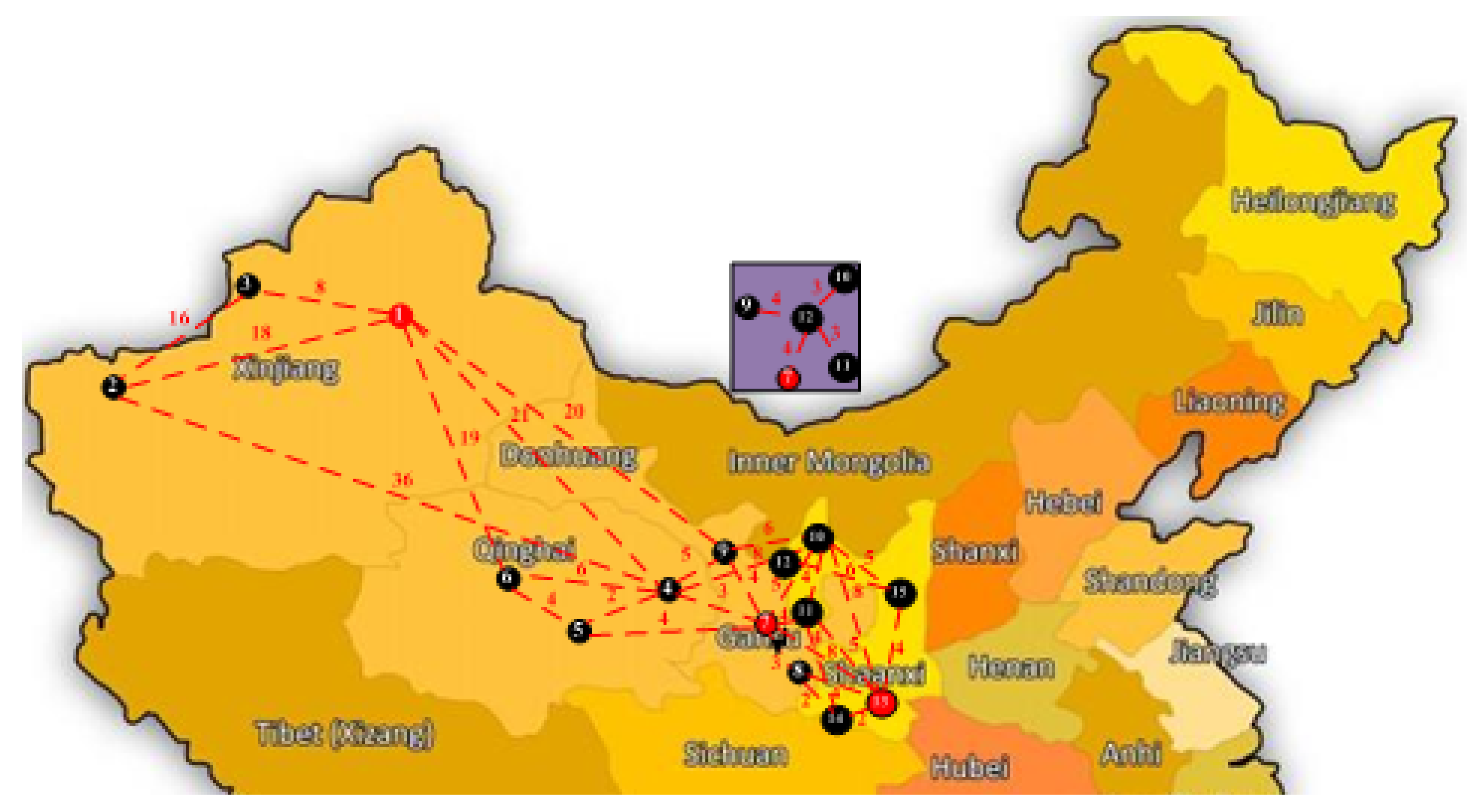
As mentioned earlier, northwest China is fruitful, and its agriculture is productive. Northwest China includes the Shaanxi, Gansu, Qinghai, Ningxia, Xinjiang provincial administrative regions. In

Table 1. Distances distribution of five provinces in northwest China (km = 1:80).

Province	City Node	(1)	(2)	(3)	(4)	(5)	(6)	(7)	(8)	(9)	(10)	(11)	(12)	(13)	(14)	(15)
Xinjiang	(1)	0	18	8	21	23	19	24	27	20	25	26	24	31	30	30
	(2)	18	0	16	36	34	30	38	42	35	41	41	39	46	44	45
	(3)	8	16	0	30	29	25	32	36	29	33	35	32	40	38	38
Qinghai	(4)	21	36	30	0	2	6	3	6	5	8	7	8	10	8	11
	(5)	23	34	29	2	0	4	4	8	4	9	8	7	12	10	13
	(6)	19	30	25	6	4	0	9	12	9	14	13	12	16	14	17
Gansu	(7)	24	38	32	3	4	9	0	3	4	5	4	4	8	6	8
	(8)	27	42	36	6	8	12	3	0	7	7	3	6	4	2	7
	(9)	20	35	29	5	4	9	4	7	0	6	6	4	11	9	9
Ningxia	(10)	25	41	33	8	9	14	5	7	6	0	4	3	8	8	5
	(11)	26	41	35	7	8	13	4	3	6	4	0	3	5	4	6
	(12)	24	39	32	8	7	12	4	6	4	3	3	0	8	6	6
Shanxi	(13)	31	46	40	10	12	16	8	4	11	8	5	8	0	2	4
	(14)	30	44	38	8	10	14	6	2	9	8	4	6	2	0	3
	(15)	30	45	38	11	13	17	8	7	9	5	6	6	4	3	0

Note (1): The 15 cities are (1) Wu-lu-mu-qi, (2) Ka-shi, (3) I-li, (4) Xi-ning, (5) Hai-nan, (6) Hai-xi,(7) Lan-zhou, (8) Tian-shui, (9) Wu-wei, (10) Yin-chuan, (11) Gu-yuan, (12) Zhong-wei, (13) Xi-an, (14) Bao-ji, (15) Yan-an. Note (2): Nodes 1, 7, and 13 as our distribution centers.

, because of the cold chain logistics costs, we assume that one can operate the routes as shown in Figure 1, where distribution of the distance of five provinces in northwest China is on a scale of 1:80 km. In addition, the actual distance data for cold chain logistics between 15 cities are measured from the Google map. We determine three cities, 1, 7, and 13, as our distribution centers, marked as red circles in Figure 1. Distribution centers 1 and 7 are located in the western region, and distribution center 13 is closer to the eastern region. It is necessary to consider the proximity of three distribution centers to other demands, and we mark the distribution centers with red circles in Figure 1. Connections between any two of the distribution centers indicate that it is feasible for these two distribution centers to connect to each other. Contrastingly, if there is no connection, it means that it is not feasible for these two distribution centers to connect. Digitals on the lines represent the distances between any two adjacent cities. To simplify the calculation, the real distances are divided by 80, and the unit of measurement is kilometers (km). In this study, we apply the Monte Carlo simulation to generate the demands of forward and return for cold chain logistics, following the uniform distribution as shown in

Table 2. The demands of the forward and return cities of the uniform distribution in the Monte Carlo simulation.

Demand Point (An)	Forward Demands (an)	Return Demands (bn)
[8,10]	[10,20]	[1,10]

. We further investigate the return loading rate problem in two manners, Long-Route and Short-Route.

Table 3. The demands of the forward and return cities of the Long-Route example in the Monte Carlo simulation.

Demand Point (An)	Forward Demands (an)	Return Demands (bn)	Load Rate (Ln) %
1	-	-	-
4	20	10	50%
5	12	7	35%
6	11	6	30%
7	-	-	-
8	15	8	40%
9	14	5	25%
10	10	6	30%
11	18	10	50%
13	-	-	-

Note: Exclusive of nodes 1, 7, and 13 as our distribution centers.

lists the Long-Route parameter setup derived by Table 2, and we denote A_n as 10 demanding cities: 1, 4, 5, 6, 7, 8, 9, 10, 11, 13. The a_n and b_n represent the demands of the forward and return cities such that a_n represents the demand to unload at this demand city; b_n represents the demands to be returned to the starting distribution center (node 1) and may also pass the interim distribution center (node 7). L_n represents the single point loading rate of each demand city calculated by Equation (7).

4.2. Mathematical Modeling

In this section, we utilize two scenarios to illustrate our proposed model. The first one is the Long-Route scenario, starting from city Wu-lu-mu-qi (city 1) to city Xi-an (end city 13) and returning to city Wu-lu-mu-qi. The second one is the Short-Route scenario, starting from city Lan-zhou (city 7) to city Xi-an (end city 13) and returning to city Lan-zhou.

4.2.1. The Illustrative Example of the Long-Route Scenario

Based on Equations (1)–(5), an initial mathematical model of return loading rate problem can be obtained by using entries of columns (1) to (5) in

Table 4. The illustrative example of the Long-Route in TOC model.

	Sub-Tour Reversal Model						TOC Model
	(1)	(2)	(3)	(4)	(5)	(6)	(7)	(8)	(9)	(10)
Iterations	Routes	M1	M2	NVm	Distance (km)	RLRm (%)	Routes	CCR	Distance (km)	RLRm (%)
1	1-6-4-7-8-13-10-11-9-1	46	21	3	73	35%	-	-	-	-
2	1-4-6-7-8-13-10-11-9-1	46	21	3	75	35%	-	-	-	-
3	1-4-6-7-8-13-11-10-9-1	46	21	3	72	35%	-	-	-	-
4	1-4-6-7-8-13-10-11-9-1	46	21	3	75	35%	-	-	-	-
5	1-4-6-7-8-13-11-10-9-1	46	21	3	72	35%	-	-	-	-
6	1-6-4-7-8-13-11-10-9-1	46	21	3	70 *	35% *	1-6-4-7-8-13-11-10-9-1	City 9 (25%)	-	-
7	-	-	-	-	70	35%	1-6-5-7-8-13-11-10-4-1	City 4 (50%)	72	60% *

. According to the initialization in Figure 1, the initial solution is 1-6-4-7-8-13-10-11-9-1 in the Long-Route scenario. In Table 4, due to the initial, random Long-Route pass through 10 cities, we measure M_1,10 = city 6 + city 4 + city 8 = 11 + 20 + 15 = 46, M_2,10 = city 10 + city 11 + city 9 = 6 + 10 + 5 = 21, NV₁₀ = 46/20 = 2.3 and maps NV₁₀ to the least integer = 3. Finally, RLR₁ = $\left[1-\left(3\cdot 20-21\right)/\left(3\cdot 20\right)\right]\cdot 100\%=35\%$. The initial distance from city 1 = 19 + 6 + 3 + 3 + 4 + 8 + 4 + 6 + 20 = 73 km and iteration 1 is completed.

Finally, we execute the step of the repeat and stop rule from the Sub-Tour reversal algorithm until iteration 6 is completed to find the optimal solution. When there is no path to reverse to improve the current solution in iteration 6 as 1-6-4-7-8-13-11-10-9-1, stopping and accepting the best answer of the distance is 70 km, and RLR₁ is 35% as the current optimal solution. We detail all the iterations in Table 4. The current optimal Long-Route in phase 1 is obtained; however, the return loading rate is not in excess of 50%. Then, we perform the following TOC model to optimize the return loading rate problem. The TOC finds the CCR city through the current, optimal Long-Route, where the demand city with the lowest single return loading rate is. According to Equation (6), L_n can be calculated in column 4 of Table 3. We get the following result:

$${\tau }_{10} =\mathrm{Min} \{\text{-}, 30\%, 45\%, \text{-}, 40\%, \text{-}, 50\%, 30\%, 25\%, \text{-}\}=25\%=\mathrm{city} 9.$$

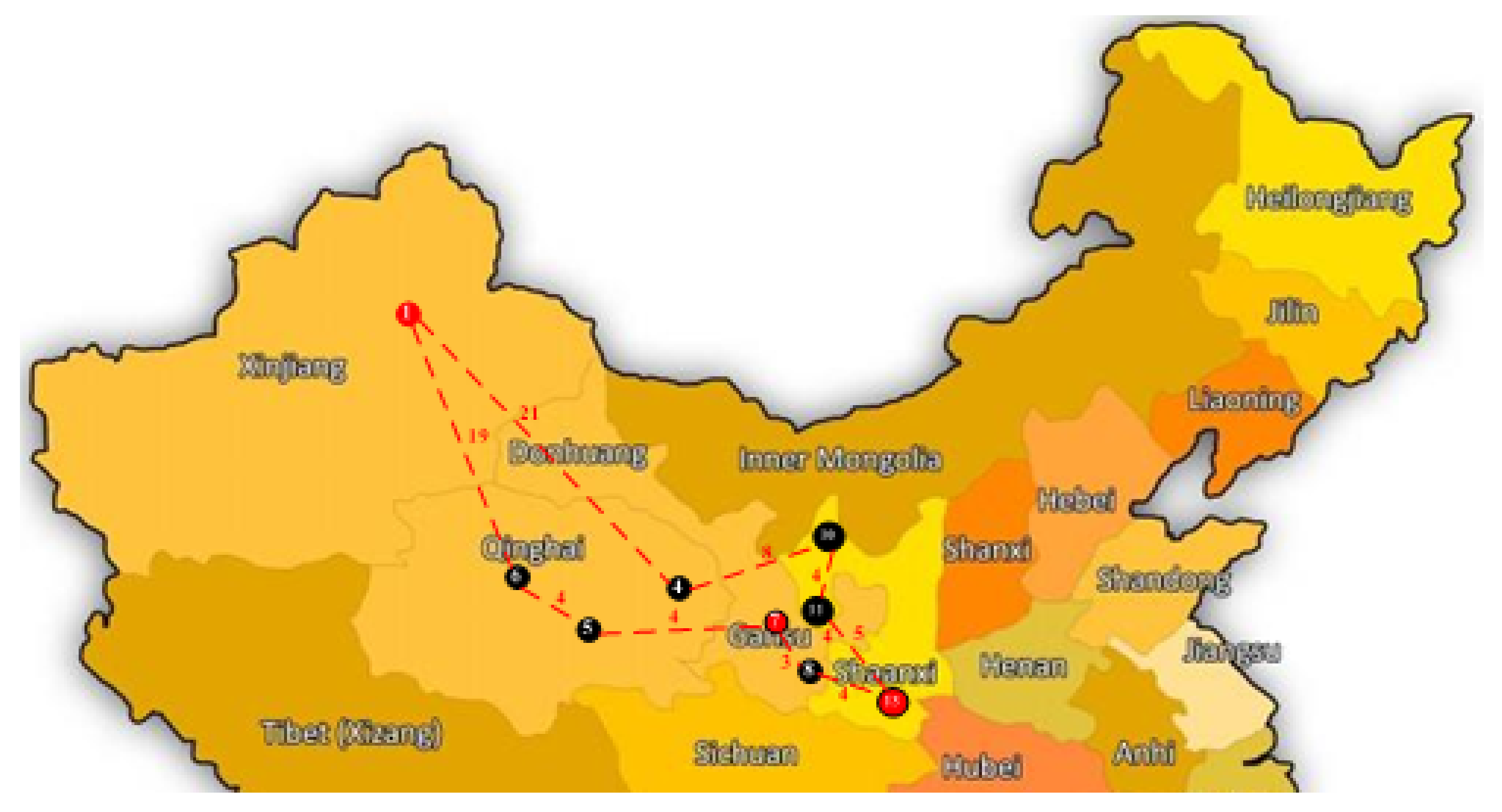
In order to substitute CCR city, we use non-CCRs cities 4 and 5 successively to replace CCR city 9 in iteration 6. Then, we obtain iteration 7 as 1-6-5-7-8-13-11-10-4-1. The solution of the total transport distance is 72 km and the current best RLR₇ is 60%, more than 50%. Thus, we obtain the optimize solution as 1-6-5-7-8-13-11-10-4-1 from the initial solution as shown in Figure 2.

4.2.2. The Illustrative Example of the Short-Route Scenario

To introduce our proposed solution procedure, we demonstrate the Short-Route in

Table 5. The demands of the forward and return cities of the Short-Route example in the Monte Carlo simulation.

Demand Point (An)	Forward Demands (an)	Return Demands (bn)	Load Rate (Ln) %
4	18	9	45%
7	-	-	-
9	13	3	15%
10	15	5	25%
11	19	7	35%
12	14	6	30%
13	-	-	-
15	19	7	35%

, where we denote A_n as 8 demanding cities: 4, 7, 9, 10, 11, 12, 13, 15. Now, suppose that the initial solution is 7-9-10-15-12-11-13-7 in the Short-Route scenario. In

Table 6. The illustrative example of the Short-Route in the TOC model.

	Sub-Tour Reversal Model						TOC Model
	(1)	(2)	(3)	(4)	(5)	(6)	(7)	(8)	(9)	(10)
Iterations	Routes	M1	M2	NVm	Distance (km)	RLRm (%)	Routes	CCR	Distance (km)	RLRm (%)
1	7-9-10-15-12-11-13-7	80	0	4	37	0%	-	-	-	-
2	7-9-10-12-15-11-13-7	80	0	4	37	0%	-	-	-	-
3	7-9-10-12-15-13-11-7	61	19	4	32	23.75%	-	-	-	-
4	7-9-10-15-12-13-11-7	61	19	4	32	23.75%	-	-	-	-
5	7-9-10-12-15-13-11-7	61	19	4	32	23.75% *	7-9-10-12-15-13-11-7	City 9 (15%)	-	-
6	-	-	-	-	32	23.75%	7-4-10-13-15-12-11-7	City 4 (45%)	36	47.5% *

, due to the initial, random Short-Route pass through 8 cities, we measured M_1,8 = city 9 + city 10 + city 15 + city 12 + city 11 = 80, M_2,10 = city 7 = 0, NV₈ = 80/20 = 4, and maps NV₈ to the least integer 4. Finally, RLR₁ = $\left[1-\left(4\cdot 20-0\right)/\left(4\cdot 20\right)\right]\cdot 100\%=0\%$. The initial distance from city 7 is 37 km, and iteration 1 is complete. Finally, we perform the Sub-Tour reversal algorithm until iteration 5 is done to find the optimal solution. When there is no path to reverse to improve the current solution in iteration 5 as 7-9-10-12-15-13-11-7, stopping and accepting the best answer of the distance is 32 km, and RLR₁ is 23.75% as the current optimal solution. We present all the iterations in Table 6. The current optimal Short-Route in phase 1 is obtained; however, the return loading rate of more than 50% is not met. We perform the TOC model to optimize the return loading rate problem. The TOC finds the CCR city through the current optimal Short-Route, where the demand city is with the lowest single return loading rate in Table 5. Then, we get the following:

$${\tau }_8=\mathrm{Min} \{\text{-}, 15\%, 25\%, 30\%, 35\%, \text{-}, 35\%, \text{-}\}=15\%=\mathrm{city} 9.$$

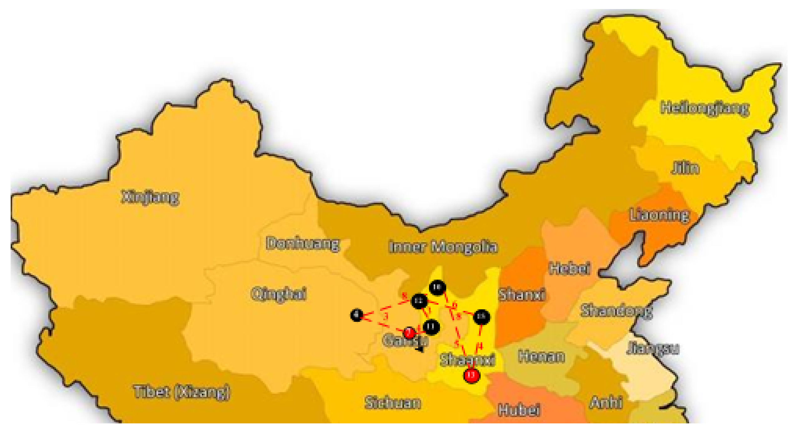
In order to avoid CCR cities, we use non-CCR city 4 to replace CCR city 9 in iteration 6. We obtain iteration 6 as 7-4-10-13-15-12-11-7. The solution of the total transport distance is 36 km and the current best RLR₆ is 47.5%, somehow less than 50%. Thus, we obtain the optimal solution as 7-4-10-13-15-12-11-7 from the initial solution as shown in Figure 3.

4.2.3. Discussion

To solve the return loading rate problem, this study further investigates the Long-Route and Short-Route scenarios. In the Long-Route scenario, Table 3 shows the demands of the forward and return cities, adopting the Monte Carlo simulation. To substitute CCR city 9, we use non-CCR city 4 with a loading rate of 50%, successively, to replace CCR city 9 with a loading rate of 25% and then determine a feasible solution that leads to the highest return loading rate of 60%. In Table 4, after iteration 6 of the Long-Route, the current best distance is 70 km, which is less than 73 km in the initial solution. This can be achieved by using the Sub-Tour reversal model and indicates a 4.1% reduction from the initial solution. However, the current best return loading rate (RLR₆) remains the same as in the initial solution, i.e., 35%. The expected goal of a return loading rate of more than 50% is not achieved by using the Sub-Tour reversal model. Therefore, we introduce the TOC model to optimize the return loading rate. By using the TOC model, we remove CCR city 9 and replace it with the higher return loading rate, i.e., non-CCR city 4. The final results indicate that as we consider the CCR city, the distance and its return loading rate are higher than the initial solution and outperform the Sub-Tour reversal model. In Figure 2, we obtain the optimal Long-Route, starting from Wu-lu-mu-qi (city 1) to Hai-xi (city 6), Hai-nan (city 5), Lan-zhou (city 7), Tian-shui (city 8), Xi-an (city 13), Gu-yuan (city 11), Yin-chuan (city 10), Xi-ning (city 4) and returning to Wu-lu-mu-qi (city 1). The optimal Long-Route derives the total transport distance of 72 km with the best return loading rate of 60%. In the Short-Route scenario, Table 5 shows the demands of the forward and return cities by applying the Monte Carlo simulation. To substitute CCR city 9, we use non-CCR city 4 with a loading rate of 45%, successively, to replace the CCR city 9 with a loading rate of 15% and then determine a feasible solution that leads to the highest return loading rate of 47.5%.

In Table 6, after iteration 1 of the Short-Route, the current best distance decreases from the initial solution of 37 km to 32 km. The current best return loading rate increases from the initial solution of 0% to 23.75%, for a 23.75% improvement via the Sub-Tour reversal model. With the goal of improving the return loading rate to more than 50%, this study achieves the goal by using the TOC model because of the final loading rate being 47.5%. The former route can be derived by the Sub-Tour reversal model but fails to meet expectations according to the results of a distance of 32 km and a return loading rate of 23.75%. Accordingly, this study achieves its goal by using the TOC model such that the final results can be a distance equal to 36 km and a return loading rate equal to 47.5%. In Figure 3, we obtain the optimal Short-Route starting from Lan-zhou (city 7) to Xi-ning (city 4), Yin-chuan (city 10), Xi-an (city 13), Yan-an (city 15), Zhong-wei (city 12), Gu-yuan (city 11) and returning to Lan-zhou (city 7). The optimal Short-Route gets the total transport distance of 36 km with the best return loading rate of 47.5%.

To see our model capability, this paper utilizes the simulation data to validate the TOC model and adopts the Monte Carlo simulation method to test the deriving solutions. Based on the resulting outcomes in

Table 7. The 30 replications simulation results of the Long-Route scenario in the Monte Carlo simulation.

	Sub-Tour Reversal Model						TOC Model
	(1)	(2)	(3)	(4)	(5)	(6)	(7)	(8)	(9)	(10)
Runs	Routes	M1	M2	NVm	Distance (km)	RLRm (%)	Routes	CCR	Distance (km)	RLRm (%)
1	1-4-12-7-8-13-11-14-5-1	42	22	3	82	36.67%	1-10-6-7-5-13-11-4-12-1	City 10	106	72.5%
2	1-2-4-10-14-13-12-9-8-1	49	10	3	118	16.67%	1-2-6-10-7-13-12-11-4-1	City 2	114	72.5%
3	1-11-6-7-3-13-14-8-4-1	46	17	3	151	28.33%	1-11-6-7-2-13-12-4-10-1	City 2	148	57.5%
4	1-7-8-12-6-13-2-15-14-1	41	10	3	185	16.67%	1-7-15-6-8-13-4-11-12-1	City 8	109	72.5%
5	1-8-2-14-4-13-6-3-12-1	49	19	3	228	31.67%	1-8-2-7-6-13-4-11-12-1	City 8	176	72.5%
6	1-2-11-3-12-13-5-8-4-1	65	17	4	181	21.25%	1-2-5-7-6-13-11-12-4-1	City 2	118	72.5%
7	1-6-7-12-5-13-10-14-2-1	45	12	3	129	20%	1-10-7-6-5-13-12-11-4-1	City 10	94	72.5%
8	1-9-4-15-10-13-12-8-14-1	49	16	3	95	26.67%	1-6-7-15-10-13-12-11-4-1	City 10	88	72.5%
9	1-15-9-2-4-13-11-14-12-1	49	25	3	159	41.67%	1-7-9-2-6-13-11-4-12-1	City 9	153	72.5%
10	1-12-14-2-5-13-10-4-8-1	61	15	4	169	18.75%	1-10-7-2-5-13-12-4-11-1	City 2	163	72.5%
11	1-11-12-7-4-13-5-3-2-1	49	11	3	121	18.33%	1-5-2-7-6-13-11-12-4-1	City 2	157	72.5%
12	1-3-9-5-2-13-15-10-12-1	54	15	3	157	25%	1-7-9-5-2-13-4-11-12-1	City 9	156	72.5%
13	1-7-8-11-3-13-4-5-6-1	45	23	3	140	38.33%	1-7-5-6-2-13-4-11-12-1	City 2	152	72.5%
14	1-10-11-9-7-13-6-5-14-1	39	19	2	107	47.5%	1-10-11-9-7-13-12-5-4-1	City 9	85	62.5%
15	1-7-11-9-15-13-12-14-6-1	44	22	3	94	36.67%	1-7-2-9-15-13-12-14-4-1	City 9	153	62.5%
16	1-12-3-11-5-13-10-7-8-1	69	5	4	154	6.25%	1-7-2-10-5-13-11-12-4-1	City 2	161	72.5%
17	1-12-7-3-2-13-5-11-15-1	48	18	3	178	30%	1-5-7-8-2-13-12-11-4-1	City 8	157	72.5%
18	1-10-15-11-7-13-9-4-8-1	42	11	3	97	18.33%	1-10-15-8-7-13-11-4-12-1	City 8	92	72.5%
19	1-6-3-9-4-13-8-14-15-1	53	9	3	127	15%	1-6-7-9-8-13-4-11-12-1	City 9	87	72.5%
20	1-15-7-10-8-13-9-14-2-1	35	8	2	136	20%	1-15-7-10-8-13-12-11-2-1	City 8	124	52.50%
21	1-5-15-3-4-13-8-9-11-1	59	11	3	157	18.33%	1-5-6-2-7-13-12-4-11-1	City 2	152	72.5%
22	1-3-11-14-5-13-6-9-4-1	66	17	4	120	21.25%	1-3-2-7-5-13-12-11-4-1	City 2	117	72.5%
23	1-15-10-3-5-13-2-14-4-1	57	18	3	228	30%	1-15-10-2-7-13-11-14-4-1	City 15	160	65%
24	1-7-10-15-6-13-8-4-5-1	36	17	2	102	42.5%	1-7-10-15-6-13-12-4-5-1	City 15	99	62.5%
25	1-3-4-10-6-13-11-5-14-1	51	22	3	129	36.67%	1-7-4-10-6-13-11-5-14-1	City 10	118	55%
26	1-11-9-2-15-13-14-3-7-1	54	9	3	180	15%	1-7-9-2-15-13-11-3-4-1	City 9	203	57.5%
27	1-10-8-4-6-13-7-2-9-1	43	2	3	161	3.33%	1-10-8-7-6-13-12-2-4-1	City 8	164	52.5%
28	1-5-12-6-14-13-3-2-7-1	62	5	4	174	6.25%	1-5-7-6-2-13-3-4-12-1	City 2	214	55%
29	1-14-3-11-10-13-12-6-7-1	62	16	4	168	20%	1-7-3-2-10-13-12-6-11-1	City 2	180	65%
30	1-11-8-3-15-13-7-6-2-1	60	9	3	139	15%	1-7-8-2-15-13-11-6-4-1	City 8	163	67.5%
				Avg.	145.53km	24.07%		Avg.	138.77km	67.33%

,

Table 8. The 30 replications simulation results of the Short-Route scenario in the Monte Carlo simulation.

	Sub-Tour Reversal Model						TOC Model
	(1)	(2)	(3)	(4)	(5)	(6)	(7)	(8)	(9)	(10)
Runs	Routes	M1	M2	NVm	Distance (km)	RLRm (%)	Routes	CCR	Distance (km)	RLRm (%)
1	7-15-8-12-13-14-10-7	45	10	3	44	16.67%	7-15-8-10-13-14-11-7	City 8	40	47.5%
2	7-12-14-10-13-15-11-7	47	12	3	40	20%	7-8-13-10-14-12-11-7	City 8	36	95%
3	7-14-15-12-13-10-11-7	52	14	3	39	23.33%	7-10-13-8-15-12-11-7	City 8	37	95%
4	7-11-8-9-13-14-10-7	39	10	2	40	16.67%	7-10-8-13-9-14-11-7	City 9	44	80%
5	7-8-9-12-13-11-15-7	42	12	3	41	20%	7-8-10-13-9-11-15-7	City 9	49	60%
6	7-10-12-9-13-8-11-7	42	11	3	34	18.33%	7-10-13-8-9-12-11-7	City 9	35	95%
7	7-8-12-14-13-11-9-7	47	10	3	32	16.67%	7-8-14-9-13-12-11-7	City 9	40	47.5%
8	7-9-11-8-13-10-12-7	39	13	2	32	32.5%	7-9-10-8-13-11-12-7	City 9	33	47.5%
9	7-10-9-8-13-11-15-7	32	12	2	41	30%	7-10-13-8-9-11-12-7	City 9	37	95%
10	7-11-10-8-13-14-15-7	37	8	2	32	20%	7-14-10-8-13-11-12-7	City 8	37	47.5%
11	7-10-11-14-13-12-8-7	44	10	3	32	16.67%	7-10-8-13-14-12-11-7	City 8	31	95%
12	7-14-9-10-13-8-12-7	39	10	2	43	16.67%	7-14-8-10-13-11-12-7	City 8	35	47.5%
13	7-8-15-14-13-12-9-7	42	9	3	31	15%	7-8-10-13-14-12-11-7	City 8	33	95%
14	7-15-14-11-13-9-12-7	49	9	3	38	15%	7-15-9-13-14-12-11-7	City 9	43	47.5%
15	7-12-8-10-13-15-11-7	40	12	2	39	30%	7-8-13-10-15-11-12-7	City 8	33	95%
16	7-10-9-14-13-15-12-7	39	11	2	36	27.5%	7-10-9-8-13-11-12-7	City 9	34	47.5%
17	7-8-11-10-13-14-15-7	37	8	2	31	20%	7-8-13-10-15-14-11-7	City 8	31	80%
18	7-15-12-8-13-11-9-7	45	10	3	39	16.67%	7-15-8-9-13-12-11-7	City 9	48	47.5%
19	7-11-9-10-13-12-8-7	39	10	2	41	16.67%	7-8-13-10-9-12-11-7	City 9	32	95%
20	7-14-15-10-13-8-11-7	42	11	3	33	18.33%	7-10-8-13-14-11-15-7	City 8	36	60%
21	7-12-14-8-13-10-11-7	47	14	3	32	23.33%	7-10-13-8-14-12-11-7	City 8	32	95%
22	7-9-15-14-13-11-8-7	44	11	3	29	18.33%	7-9-15-13-14-11-12-7	City 9	30	47.5%
23	7-11-8-14-13-9-12-7	44	9	3	30	15%	7-9-8-14-13-11-12-7	City 9	27	47.5%
24	7-9-14-10-13-15-12-7	39	11	2	43	27.5%	7-9-14-10-13-11-12-7	City 9	41	47.5%
25	7-8-9-10-13-15-11-7	32	12	2	38	30%	7-8-13-10-9-15-11-7	City 9	40	60%
26	7-15-8-11-13-10-12-7	42	13	3	38	21.67%	7-15-8-10-13-11-12-7	City 8	42	47.5%
27	7-12-9-8-13-15-11-7	42	12	3	33	20%	7-9-15-8-13-11-12-7	City 9	36	47.5%
28	7-10-12-15-13-11-9-7	45	10	3	33	16.67%	7-10-9-15-13-11-12-7	City 9	36	47.5%
29	7-15-12-9-13-10-14-7	47	10	3	43	16.67%	7-15-10-9-13-12-14-7	City 9	50	37.5%
30	7-15-11-8-13-12-10-7	42	13	3	37	21.67%	7-15-10-8-13-12-11-7	City 8	39	47.5%
				Avg.	36.47km	20.59%		Avg.	37.23km	64.83%

and

Table 9. The pair t-test result.

	Pair Difference		t Statistics	p Value	df
	Mean	Std. Deviation
(1) Long-Route scenario	0.4326	0.1294	18.3190	0.001 <	29
(2) Short-Route scenario	0.4425	0.2199	11.0203	0.001 <	29

, the TOC model effectively obtains the best routes design. Later, we discuss the simulation and its statistics in detail.

4.2.4. The Simulation and Its Statistics

Furthermore, this paper utilizes the simulation data to validate our model and adopts the Monte Carlo simulation method, following the uniform distribution in Table 2 to test the deriving solutions. It simulates 30 replications of datasets for certain demand cities (A_n) 10 and 8, forward (a_n) with a range between 10 and 20 tons and a return (b_n) with a range between 1 and 10 tons in Table 2. By our proposed model, we summarize our results as shown in Table 7 and Table 8.

We know that the average return loading rate derived by the Sub-Tour reversal model is 24.07% and by TOC model, it is 67.33%, based on northwest China’s Long-Route scenario shown in Table 7. This study further employs the pair t-test to see whether the mean difference is significant or not. Based on the data, the t statistic is 18.3190 and the p value is less than 0.05. It means that there exists a significant difference among the two models, and our model leads to an improvement of 43.26% compared to that obtained by the Sub-Tour reversal model. Following the same procedure, the TOC model results in an improvement of 44.02%, comparing to that obtained by the Sub-Tour reversal model from the Short-Route scenario in Table 8. The t statistic is 11.0204 and the p value is less than 0.05. Obviously, our proposed solution procedure can be applied to solve the return loading rate problem in an efficient manner. The resulting outcomes are arranged in Table 9. By the resulting outcomes, our proposed solution procedure successfully integrates the Sub-Tour reversal model and TOC. The results show the superiority of the TOC model in solving issues in logistics and answering the question mentioned by previous studies (see Schragenheim and Dettmer [24]; Lee et al. [13]; Chang and Huang [14]; Benavides and Landeghem [25]; Chakravorty and Hales [26]). The TOC model achieves the logistics goal for increasing the return loading rate by increasing by more than 50%. Logistics companies would benefit substantially from the application of the TOC model.

5. Conclusions

This study intends to propose a solution procedure to reduce the total transportation distance and to improve the return transportation vehicle loading rate by more than 50% in northern China. Our research contributes to developing the model considering two factors: the total transportation distance and the return loading rates of transport vehicles, which are different from previous studies mainly focusing on minimizing total logistics costs. The TOC model further optimizes the results of the Sub-Tour reversal method to determine the degree of improvement resulted from the TOC model. Based on bottleneck orientation, this paper broadens the view of the existing research field. We integrated the Sub-Tour reversal model and the TOC methodology, as the two-phase solution procedure solves the problem of the return loading rate. Usually, the Sub-Tour reversal model is applied to solve the minimization transportation distance problem. Our model adopts the deriving results of the Sub-Tour reversal model as the initial solution. Next, we applied the TOC model, employing the CCR concept to further optimize the current solution since the TOC model can quickly locate the CCR city (i.e., lowest return loading rate) and accurately find the limitations of the route. It should be noted that to find the optimal solution by maximizing the utility of the CCR in this study means replacing the CCR city with a non-CCR. In order to demonstrate our model capability, we further utilized two scenarios and employed the Monte Carlo simulation. In the northwest logistics network design, as presented in Table 7 and Table 8, the return loading rate is significantly improved by our proposed solution procedure, and this shows that our proposed model outperforms the conventional Sub-Tour reversal method. Note that our solution procedure can be implemented in real-world situations in a simple manner. The limitations of the study are calculating the total logistics costs of the optimized transportation distance. For future work, we suggest a number of issues for future researchers. (1) Our research investigated the deterministic manner. For future investigations, we may take uncertainty factors into account. (2) Our future model would further consider other factors, such as environmental protection, carbon pricing or emission. (3) In this research, we integrated the Sub-Tour reversal model with TOC. We can employ other approaches in future research.

References

- Subulan, K.; Baykasoğlu, A.; Saltabas, A. An improved decoding procedure and seeker optimization algorithm for reverse logistics network design problem. J. Intell. Fuzzy Syst. 2014, 27, 2703–2714. [Google Scholar] [CrossRef]
- Soysal, M.; Bloemhof-Ruwaard, J.M.; van der Vorst, J.G.A.J. Modelling food logistics networks with emission considerations: The case of an international beef supply chain. Int. J. Prod. Econ. 2014, 152, 57–70. [Google Scholar] [CrossRef]
- Kim, J.S.; Lee, D.L. An integrated approach for collection network design, capacity planning and vehicle routing in reverse logistics. J. Oper. Res. Soc. 2015, 66, 76–85. [Google Scholar] [CrossRef]
- Konstantakopoulos, G.D.; Gayialis, S.P.; Kechagias, E.P. Vehicle routing problem and related algorithms for logistics distribution: A literature review and classification. Oper. Res. 2020, 1–30. [Google Scholar] [CrossRef]
- Hillier, F.S.; Lieberman, G.J. Introduction to Operations Research; McGraw-Hill, Inc.: New York, NY, USA, 2006. [Google Scholar]
- Moroko, W.; Caflisch, R. Quasi-Monte Carlo Simulation of Random Walks in Finance. In Athens Conference on Applied Probability and Time Series Analysis; Niederreiter, H., Hellekalek, P., Larcher, G., Zinterhof, P., Eds.; Springer: New York, NY, USA, 1998; Volume 127, pp. 340–352. [Google Scholar]
- Huang, W.-T.; Chen, P.-S.; Liu, J.J.; Chen, Y.-R.; Chen, Y.-H. Dynamic configuration scheduling problem for stochastic medical resources. J. Biomed. Inform. 2018, 80, 96–105. [Google Scholar] [CrossRef]
- Daganzo, C.F. The distance traveled to visit n points with a maximum of c stops per vehicle: An analytic model and an application. Transp. Sci. 1984, 18, 331–350. [Google Scholar] [CrossRef] [Green Version]
- Dobos, I. Optimal production–inventory strategies for a HMMS-type reverse logistics system. Int. J. Prod. Econ. 2003, 81-82, 351–360. [Google Scholar] [CrossRef]
- Ljungberg, D.; Gebresenbet, G. Mapping out the potential for coordinated goods distribution in city centres: The case of Uppsala. Int. J. Transp. Manag. 2004, 2, 161–172. [Google Scholar] [CrossRef]
- Guo, R.; Guan, W.; Zhang, W. Route design problem of customized buses: Mixed integer programming model and case study. J. Transp. Eng. Part A Syst. 2018, 144, 04018069. [Google Scholar] [CrossRef]
- Wang, C.-N.; Nguyen, N.-A.-T.; Dang, T.-T.; Lu, C.-M. A Compromised Decision-Making Approach to Third-Party Logistics Selection in Sustainable Supply Chain Using Fuzzy AHP and Fuzzy VIKOR Methods. Mathematics 2021, 9, 886. [Google Scholar] [CrossRef]
- Duan, S.X.; Wibowo, S.; Chong, J. A multicriteria analysis approach for evaluating the performance of agriculture decision support systems for sustainable agribusiness. Mathematics 2021, 9, 884. [Google Scholar] [CrossRef]
- Jiang, X.; Zhou, J. The Impact of Rebate Distribution on Fairness Concerns in Supply Chains. Mathematics 2021, 9, 778. [Google Scholar] [CrossRef]
- Paksoy, T.; Bektaş, T.; Özceylan, E. Operational and environmental performance measures in a multi-product closed-loop supply chain. Transp. Res. Part E: Logist. Transp. Rev. 2011, 47, 532–546. [Google Scholar] [CrossRef]
- Fahimnia, B.; Reisi, M.; Paksoy, T.; Özceylan, E. The implications of carbon pricing in Australia: An industrial logistics planning case study. Transp. Res. Part D: Transp. Environ. 2013, 18, 78–85. [Google Scholar] [CrossRef]
- Özceylan, E.; Paksoy, T.; Bektas, T. Modeling and optimizing the integrated problem of closed-loop supply chain network design and disassembly line balancing. Transp. Res. Part E Logist. Transp. Rev. 2014, 61, 142–164. [Google Scholar] [CrossRef]
- Özceylan, E.; Demirel, N.; Çetinkaya, C.; Demirel, E. A closed-loop supply chain network design for automotive industry in Turkey. Comput. Ind. Eng. 2017, 113, 727–745. [Google Scholar] [CrossRef]
- Çil, Z.A.; Li, Z.; Mete, S.; Özceylan, E. Mathematical model and bee algorithms for mixed-model assembly line balancing problem with physical human–robot collaboration. Appl. Soft Comput. 2020, 93, 106394. [Google Scholar] [CrossRef]
- Miraç, E.; Özceylan, E. P-median and maximum coverage models for optimization of distribution plans: A case of United Nations Humanitarian response depots. In Smart and Sustainable Supply Chain and Logistics—Trends, Challenges, Methods and Best Practices; Golinska-Dawson, P., Tsai, K.M., Kosacka-Olejnik, M., Eds.; EcoProduction (Environmental Issues in Logistics and Manufacturing); Springer: Cham, Switzerland, 2020. [Google Scholar]
- Ryu, B.W.; Hyun, P.J. The study of logistics optimization model with empty transfer rate of reverse logistics. J. Korea Saf. Manag. Sci. 2006, 8, 125–141. [Google Scholar]
- Lee, J.-H.; Chang, J.-G.; Tsai, C.-H.; Li, R.-K. Research on enhancement of TOC Simplified Drum-Buffer-Rope system using novel generic procedures. Expert Syst. Appl. 2010, 37, 3747–3754. [Google Scholar] [CrossRef]
- Chang, Y.-C.; Huang, W.-T. An enhanced model for SDBR in a random reentrant flow shop environment. Int. J. Prod. Res. 2014, 52, 1808–1826. [Google Scholar] [CrossRef]
- Schragenheim, E.; Dettmer, H.W. Manufacturing at Warp Speed: Optimizing Supply Chain Financial Performance; CRC Press: Boca Raton, FL, USA, 2000. [Google Scholar]
- Benavides, M.B.; Landeghem, H.V. Implementation of S-DBR in four manufacturing SMEs: A research case study. Prod. Plan. Control 2015, 26, 1110–1127. [Google Scholar] [CrossRef]
- Chakravorty, S.S.; Hales, D.N. Improving labor relations performance using a Simplified Drum Buffer Rope (S-DBR) technique. Prod. Plan. Control 2016, 27, 102–113. [Google Scholar] [CrossRef] [Green Version]
Figure 1.
The northwest regional distribution centers and cities’ distance (Km = 1:80).
Figure 2.
The optimizing solution of Long-Route scenario in TOC (Km = 1:80).
Figure 3.
The optimizing solution of Short-Route scenario in TOC (km = 1:80).