Damped Newton Stochastic Gradient Descent Method for Neural Networks Training

Abstract

First-order methods such as stochastic gradient descent (SGD) have recently become popular optimization methods to train deep neural networks (DNNs) for good generalization; however, they need a long training time. Second-order methods which can lower the training time are scarcely used on account of their overpriced computing cost to obtain the second-order information. Thus, many works have approximated the Hessian matrix to cut the cost of computing while the approximate Hessian matrix has large deviation. In this paper, we explore the convexity of the Hessian matrix of partial parameters and propose the damped Newton stochastic gradient descent (DN-SGD) method and stochastic gradient descent damped Newton (SGD-DN) method to train DNNs for regression problems with mean square error (MSE) and classification problems with cross-entropy loss (CEL). In contrast to other second-order methods for estimating the Hessian matrix of all parameters, our methods only accurately compute a small part of the parameters, which greatly reduces the computational cost and makes the convergence of the learning process much faster and more accurate than SGD and Adagrad. Several numerical experiments on real datasets were performed to verify the effectiveness of our methods for regression and classification problems.

1. Introduction

First-order methods are popularly used to train deep neural networks (DNNs), such as stochastic gradient descent (SGD) [1] and its variants which use momentum and acceleration [2] and an adaptive learning rate [3]. At each iteration, SGD calculates the gradient on only a small batch instead of the whole training data. Such randomness introduced by sampling the small batch can lead to the better generalization of the DNNs [4]. Recently, there is a lot of work attempting to come up with more efficient first-order methods beyond SGD [5]. First-order methods are easy to implement and only require moderate computational cost per iteration; however, the requirement of adjusting their hyper-parameters (such as learning rate) becomes a complex task, and they are often slow to flee from areas when the loss function’s Hessian matrix is ill-conditioned [6].

Second-order stochastic methods were also proposed for training DNNs because they take far fewer iterations. Second-order stochastic methods especially have the ability to escape from regions where the Hessian matrix of the loss function is ill-conditioned and provide adaptive learning rates. However, the main problem here is that it is practically impossible to compute and invert a full Hessian matrix due to the massive parameters of DNNs and the Hessian matrix is not always positive definite  [7]. Efforts to conquer this problem include Kronecker-factored approximate [8,9,10], Hessian-free inexact Newton methods [11,12,13,14], stochastic L-BFGS methods, Gauss–Newton [15] and natural gradient methods [16,17,18] and diagonal scaling methods [19] which cut the cost by approximating the Hessian matrix. In addition, at the base of these methods, more algorithms are generated, such as SMW-GN and SMW-NG, which use the Sherman–Morrison–Woodbury formula to cut the cost of computing the inverse matrix [20] and GGN that combining GN and NTK [21]. There are also some variances of the Quasi–Newton methods for approximating the Hessian matrix [22,23,24,25]. However, most of these second-order methods lose too much information of the Hessian matrix. They lose a part of information by obtaining the approximate Hessian matrix, and further loss by adding regular terms to make the Hessian matrix positive definite.

1.1. Our Contributions

Our main contribution is the development of methods to train DNNs that combine first-order information and some second-order information, while keeping the computational cost of each iteration comparable to that required by first-order methods. To achieve this, we propose new damped Newton stochastic gradient descent methods that can be efficiently implemented. Our methods adjust the iteration of SGD by changing the iteration of the parameters of the last layer of DNNs. We used the damped Newton method for the iteration of the parameters of the last layer of DNNs, which makes the loss function decrease more rapidly. In addition, a quicker descent can exceed the cost of computing the Hessian matrix of the parameters of the layer. We elaborated the availability of our methods with numerical experiments, and compared these with those of the first-order method (SGD) and Adagrad.

The novelty of our work is that we computed the Hessian matrices of the last layer parameters and the penultimate layer of the loss function by mathematical formula and mathematically and rigorously demonstrated that the Hessian matrices are positive semi-definite. Furthermore, we then propose the DN-SGD and SGD-DN algorithms, which let the parameters of the last layer iterate with the variational damped Newton method.

To the best of our knowledge, we were the first to directly calculate the loss function of the last layer and the penultimate layer parameters of the Hessian matrix with mathematical expressions, and demonstrate the property of the semi-positive definite of the Hessian matrix, and then use the property of the semi-positive definite to put forward our algorithms. Most other works have sought to approximate the whole Hessian matrix of all parameters by various methods, and then make it positive definite by adding a quantitative matrix.

1.2. Related Work

SMW-GN and SMW-NG [20] adjust the Gauss–Newton method (GN) and natural gradient method (NG) which use the Sherman–Morrison–Woodbury (SMW) formula to compute the inverse matrix to cut the cost of computing second-order information. Goldfarb [22] approximates the Hessian matrix by a block-diagonal matrix and uses the structure of the gradient and Hessian to further approximate these blocks, each of which corresponds to a layer, as the Kronecker product of two much smaller matrices. KF-QN-CNN [23] approximates the Hessian matrix by a layer-wise block diagonal matrix and each layer’s diagonal block is further approximated by a Kronecker product corresponding to the structure of the Hessian restricted to that layer.

The Adagrad algorithm [3] individually adapts to the learning rate of all model parameters by scaling all model parameters inversely to the square root of the sum of their historical square values. The learning rate of the parameter with the largest loss partial derivative decreases rapidly, while the learning rate of the parameter with the smallest partial derivative decreases relatively little. The net effect is a greater advance in the flat direction of the parameter space [26].

2. Main Results

2.1. Feed-Forward Neural Networks

Consider a simple fully connected neural network with $L+1$ layers. For each layer, the number of nodes is $n_l,0\le l\le L$. In the following expressions, we put the bias into the weights for simplicity. Given an input x, add a component for x to make the input as $x^{\left(0\right)}={(1,x^T)}^T$ for the first layer. For the l-th layer, add a component for $x^{(l-1)}$, so $x^{\left(l\right)}={\sigma }^{\left(l\right)}\left(W^{\left(l\right)}{x}^{(l-1)}\right)$, where $W^{\left(l\right)}={(w_1^{\left(l\right)},w_2^{\left(l\right)},\dots ,w_{n_l}^{\left(l\right)})}^T\in R^{n_l\times (n_{l-1}+1)},w_j^{\left(l\right)}={(w_{0j}^{\left(l\right)},w_{1j}^{\left(l\right)},\dots ,w_{n_{l-1}j}^{\left(l\right)})}^T\in R^{n_{l-1}+1}$ which denote the parameters between the $(l-1)$-th layer and the j-th node of l-th layer, ${\sigma }^{\left(l\right)}:R\to R$ is a nonlinear activation function and when ${\sigma }^{\left(l\right)}$ is used on a vector, which means ${\sigma }^{\left(l\right)}$ operates on every component of the vector, and the output $f(\theta ,x)={\sigma }^{\left(L\right)}\left(W^{\left(L\right)}{x}^{(L-1)}\right)$ where $\theta ={\left(\mathrm{vec}({(W^{\left(1\right)})}^T),\mathrm{vec}({(W^{\left(2\right)})}^T),\dots ,\mathrm{vec}({(W^{\left(L\right)})}^T)\right)}^T$ in which $\mathrm{vec}\left(W\right)$ vectorizes the matrix W by concatenating its columns.

Given the training data $(\mathit{X},\mathit{Y})=\{(x_1,y_1),(x_2,y_2),\dots ,(x_m,y_m)\}$, for training the neural networks, the loss function for minimization is generally defined as

$$L\left(\theta \right)={\displaystyle \frac{1}{m}}\sum _{i=1}^m{L}_i(\theta ,\mathit{X},\mathit{Y})={\displaystyle \frac{1}{m}}\sum _{i=1}^{m}l(f(\theta ,x_i),y_i),$$

(1)

where $l(f(\theta ,x_i),y_i)$ is a loss function. For the learning tasks, the standard mean square error (MSE) is always used for the regression problems and the cross-entropy loss (CEL) is used for the classification problems. Note $\theta \in R^n$ where $n={\sum }_{i=1}^L{n}_l(n_{l-1}+1)$.

2.2. Convexity of Partial Parameters of the Loss Function

Theorem 1.

Given a neural network such as the one above using MSE for a loss function of regression problems, then the number of the nodes for the L-th layer is one. In the last layer, the activation function is used as identical function for regression problems. Then, the Hessian matrix of $L\left(\theta \right)$ to the parameters of last layer is positive semi-definite. When ${\sigma }^{(L-1)}\left(x\right)=relu\left(x\right)=max(0,x)$, the Hessian matrix of $L\left(\theta \right)$ to the parameters of last but one layer is also positive semi-definite.

Proof of Theorem 1

For simplicity, consider one single input first. Given the input $x_i$, the loss function should be:

$$L(W^{\left(L\right)})={\left(W^{\left(L\right)}{x}_i^{(L-1)}-y_i\right)}^2$$

and its gradient vector as well as Hessian matrix should be:

$${\displaystyle \frac{\partial L\left(W^{\left(L\right)}\right)}{\partial W^{\left(L\right)}}}=2\left(W^{\left(L\right)}{x}_i^{(L-1)}-y_i\right)x_i^{(L-1)},$$

(2)

$${\displaystyle \frac{{\partial }^{2}L\left(W^{\left(L\right)}\right)}{\partial {\left(W^{\left(L\right)}\right)}^2}}=2x_i^{(L-1)}{\left(x_i^{(L-1)}\right)}^T=A.$$

(3)

With the knowledge of matrix [27], if $x_i^{(L-1)}$ is not a null vector, it can easily be obtained that A is a positive semi-definite matrix with rank one. As for multiple inputs, the Hessian is the addition of several positive semi-definite matrices, so the Hessian matrix is also positive semi-definite.

If the activation function ${\sigma }^{(L-1)}\left(x\right)=max(0,x)$, we can obtained the loss function:

$$L(W^{(L-1)})={(W^{\left(L\right)}{\sigma }^{(L-1)}(W^{(L-1)}{x}_i^{(L-2)})-y_i)}^2$$

and the gradient vector as well as the Hessian matrix:

$${\displaystyle \frac{\partial L}{\partial w_j^{(L-1)}}}=2(W^{\left(L\right)}{\sigma }^{(L-1)}(W^{(L-1)}{x}_i^{(L-2)})-y_i)W_j^{\left(L\right)}{\sigma }^{{}^{\prime }}({(w_j^{(L-1)})}^T{x}_i^{(L-2)})x_i^{(L-2)},$$

(4)

$${\displaystyle \frac{{\partial }^{2}L}{\partial w_j^{(L-1)}\partial w_k^{(L-1)}}}=2W_j^{\left(L\right)}{W}_k^{\left(L\right)}{\sigma }^{{}^{\prime }}({(w_j^{(L-1)})}^T{x}_i^{(L-2)}){\sigma }^{{}^{\prime }}({(w_k^{(L-1)})}^T{x}_i^{(L-2)})x_i^{(L-2)}{(x_i^{(L-2)})}^T,$$

(5)

$${\displaystyle \frac{{\partial }^{2}L}{\partial {\left(v^{L-1}\right)}^2}}=B⨂C,$$

(6)

where ⨂ denotes Kronecker product and:

$$v^{(L-1)}={({(w_1^{(L-1)})}^T,{(w_2^{(L-1)})}^T,\cdots ,{(w_{n_{L-1}}^{(L-1)})}^T)}^T,$$

$$B\in R^{n_{L-1}\times n_{L-1}},B_{jk}=2W_j^{\left(L\right)}{W}_k^{\left(L\right)}{\sigma }^{{}^{\prime }}({(w_j^{(L-1)})}^T{x}_i^{(L-2)}){\sigma }^{{}^{\prime }}({(w_k^{(L-1)})}^T{x}_i^{(L-2)}),$$

$$C=x_i^{(L-2)}{(x_i^{(L-2)})}^T.$$

Let $u_j=W_j^{\left(L\right)}{\sigma }^{{}^{\prime }}({(w_k^{(L-1)})}^T{x}_i^{(L-2)}),u={(u_1,u_2,\cdots ,u_{n_{L-1}})}^T$, we can obtain $B=2u{u}^T$. Thus, it is easy to see that B and C are positive semi-definite matrix. Since the Kronecker product of positive semi-definite matrices is also positive semi-definite [28], the Hessian matrix $B⨂C$ is positive semi-definite. Hence, the Hessian of the multiple inputs is also positive semi-definite.    □

Theorem 2.

We take a neural network such as the one above using CEL for loss function of classification problems. In the last layer, $softmax$ is used as an activation function for classification problems. Then, the Hessian matrix of $L\left(\theta \right)$ to the parameters of last layer is positive semi-definite.

Proof of Theorem 2

For simplicity, consider one single input first. Given the input $x_i$, the loss function should be:

$$L=-\sum _{j=1}^{n_L}{Y}_{j}ln{x}_{ij}^{\left(L\right)},$$

where $Y_j$ is 1 when $x_i$ is the j-th class, otherwise 0. $x_{ij}^{\left(L\right)}={\displaystyle \frac{e^{{(w_j^{\left(L\right)})}^T{x}_i^{(L-1)}}}{{\sum }_{j=1}^{n_L}{e}^{{(w_j^{\left(L\right)})}^T{x}_i^{(L-1)}}}},$ so

$$L=-\sum _{j=1}^{n_L}{Y}_j{(w_j^{\left(L\right)})}^T{x}_i^{(L-1)}+ln\left(D\right),$$

where $D={\sum }_{j=1}^{n_L}{e}^{{(w_j^{\left(L\right)})}^T{x}_i^{(L-1)}}.$

Then, compute the gradient vector as well as Hessian matrix:

$${\displaystyle \frac{\partial L}{\partial w_j^{\left(L\right)}}}=\left({\displaystyle \frac{e^{{(w_j^{\left(L\right)})}^T{x}_i^{(L-1)}}}{D}}-Y_j\right)x_i^{(L-1)},$$

(7)

$${\displaystyle \frac{{\partial }^{2}L}{\partial w_j^{\left(L\right)}\partial w_k^{\left(L\right)}}}=\left\{\begin{array}{c}{\displaystyle \frac{e^{{(w_j^{\left(L\right)})}^T{x}_i^{(L-1)}}(D-e^{{(w_j^{\left(L\right)})}^T{x}_i^{(L-1)}})}{D^2}}{x}_i^{(L-1)}{(x_i^{(L-1)})}^T,j=k,\hfill \\ -{\displaystyle \frac{e^{{(w_j^{\left(L\right)})}^T{x}_i^{(L-1)}}{e}^{{(w_k^{\left(L\right)})}^T{x}_i^{(L-1)}}}{D^2}}{x}_i^{(L-1)}{(x_i^{(L-1)})}^T,j\ne k.\hfill \end{array}\right.$$

(8)

Let $v^{\left(L\right)}={({(w_1^{\left(L\right)})}^T,{(w_2^{\left(L\right)})}^T,\dots ,{(w_{n_L}^{\left(L\right)})}^T)}^T,$ then we have:

$${\displaystyle \frac{{\partial }^{2}L}{\partial {\left(v^{\left(L\right)}\right)}^2}}=E⨂F,$$

(9)

where:

$$F={\displaystyle \frac{1}{D^2}}{x}_i^{(L-1)}{(x_i^{(L-1)})}^T,$$

$$E\in R^{n_L\times n_L},E_{jk}=\left\{\begin{array}{c}{e}^{{(w_j^{\left(L\right)})}^T{x}_i^{(L-1)}}(D-e^{{(w_j^{\left(L\right)})}^T{x}_i^{(L-1)}}),j=k,\hfill \\ -e^{{(w_j^{\left(L\right)})}^T{x}_i^{(L-1)}}{e}^{{(w_k^{\left(L\right)})}^T{x}_i^{(L-1)}},j\ne k.\hfill \end{array}\right.$$

(10)

For any vector $z={(z_1,z_2,\cdots ,z_{n_L})}^T\in R^{n_L}:$

$$z^{T}Ez=\sum _{jk}^{n_L}{z}_j{z}_k{E}_{jk}={\displaystyle \frac{1}{2}}\sum _{jk}^{n_L}{e}^{{(w_j^{\left(L\right)})}^T{x}_i^{(L-1)}}{e}^{{(w_k^{\left(L\right)})}^T{x}_i^{(L-1)}}{(z_j-z_k)}^2\ge 0.$$

(11)

Thus, E and F are positive semi-definite matrices. Because the Kronecker product of positive semi-definite matrices is also positive semi-definite [28], the Hessian matrix $E⨂F$ is positive semi-definite and the Hessian matrix of the condition of multiple inputs is also positive semi-definite.    □

3. Our Innovation: Damped Newton Stochastic Gradient Descent

As for the property of the loss function, the convexity of the loss function can be determined for the last layer of DNNs. Thus, we can use the damped Newton method for the parameters of the last layer and SGD for other layers. For each iteration, if the damped Newton method is used before SGD, it is called damped Newton stochastic gradient descent (DN-SGD). Otherwise, if SGD is used before the damped Newton method, wit is called stochastic gradient descent damped Newton method (SGD-DN).

The difficulty of neural network optimization is that the loss function is a non-convex function and there is no good method for the optimization of a non-convex function. One of the methods commonly used at present is the stochastic gradient descent method, however, the speed of the gradient descent method is slow. Our method improves the stochastic gradient descent method and accelerates its convergence speed.

Our method combines the advantages of the stochastic gradient descent and damped Newton. On the one hand, the main part of the parameters of DNNs using the SGD method for training guarantees that the computing cost changes little. On the other hand, the parameters of the last layer using DN-SGD or SGD-DN for training can make the learning process converge more quickly with just a little more computing cost. When the training data are numerous, a lesser number of iterations can significantly cut time for training the DNNs and overcome the cost of computing the second-order information of the last layer.

3.1. Defect of Methods Approximating the Hessian Matrix

The quasi-Newton method, similarly to others, approximates the Hessian matrix to cut the computing cost, however, all these methods consider the whole Hessian matrix and lose significant information to approximate. In addition, they add the scalar matrix to make the Hessian matrix positive definite.

In traditional damped Newton method, adding scalar matrix is also used to make the Hessian matrix positive definite. The iteration is

$${\theta }^{(t+1)}={\theta }^{\left(t\right)}-{(H^{\left(t\right)}+\lambda I)}^{-1}{g}^{\left(t\right)}.$$

This method is hard to put into practice for the uncertainty of $\lambda$. We cannot know the eigenvalues of the Hessian matrix so that we cannot precisely set $\lambda$. If $\lambda$ is set too big, the Hessian matrix is close to a scalar matri; however, if $\lambda$ is too small, the Hessian matrix is not sufficient to be positive definite.

3.2. Set $\lambda$ Precisely

Our optimization method was based on a more elaborated analysis for the Hessian matrix, in which the Hessian matrix was not entirely used for accelerating the training. We only used the last layer’s Hessian matrix by damped Newton method. The iteration was

$${\theta }^{(t+1)}={\theta }^{\left(t\right)}-{(H^{\left(t\right)}+\lambda I)}^{-1}{g}^{\left(t\right)},$$

where $\lambda =\beta H_{max}^{\left(t\right)}+\alpha$ in which $H_{max}^{\left(t\right)}$ is the maximum value of the element of the $H^{\left(t\right)}$ and $\alpha$ is the damping coefficient. $H_{max}^{\left(t\right)}$ is to make the matrix positive definite and lower the conditional number at the same time, and $\beta$ is to more precisely adjust the conditional number. $\alpha$ is only to prevent the condition that $H^{\left(t\right)}$ is too bad to be a null matrix or very close to a null matrix, such as the results obtained for the dataset of Shot Selection.

3.3. Last Layer Makes Front Layers Converge Better

We use the chain rule to obtain:

$${\delta }^{\left(l\right)}=(w^{(l+1)T}{\delta }^{(l+1)})\odot {\sigma }^{{}^{\prime }}(x^{\left(l\right)}),$$

where ${\delta }^{\left(l\right)}={\displaystyle \frac{\partial L}{\partial x^{\left(l\right)}}}$. We use the damped Newton method to train the last layer so that they can quickly obtain the stationary point. When the parameters of the last layer almost obtain the stationary point, the gradient almost turns zero. Thus, the gradient of the parameters of front layers are almost zero, so that they also almost the stationary point.

4. Algorithm

In this section, the DN-SGD and SGD-DN methods are summarized in Algorithms 1 and 2.

Algorithm 1: DN-SGD.

Input: Training Set $S_M=\{(x_1,y_1),(x_2,y_2),\dots ,(x_M,y_M)\}$, hyper-parameter $\beta$, $\alpha$, learning rate l, batchsize N 1 Initialize the network parameter ${\theta }^{\left(0\right)},t=0$ 2 for$t=0,1,2,\dots$do 3  Randomly select a mini-batch $S_N\subset S_M$ of size N 4  Compute $H_{last}^{\left(t\right)},g_{last}^{\left(t\right)}$ for the last layer and $H_{max}^{\left(t\right)}=max(H_{last}^{\left(t\right)})$ 5  Compute $p^{\left(t\right)}={(H_{last}^{\left(t\right)}+\lambda I)}^{-1},\lambda =\beta H_{max}^{\left(t\right)}+\alpha$ 6  Set ${\theta }_{last}^{(t+1)}={\theta }_{last}^{(t+1)}-p^{\left(t\right)}{g}_{last}^{\left(t\right)}$ 7  Compute $g_{front}^{\left(t\right)}$ for other layers 8  Set ${\theta }_{front}^{(t+1)}={\theta }_{front}^{\left(t\right)}-l{g}_{front}^{\left(t\right)}$ 9 end for

The only difference between the DN-SGD (Algorithm 1) and SGD-DN (Algorithm 2) methods is that in each iteration, the damped Newton method or the stochastic gradient descent is used first.

5. Numerical Example

5.1. Regression Problem

The performance of the algorithms DN-SGD and SGD-DN was compared with SGD and Adagrad, and the experiments were performed on several regression problems, and both training loss and testing loss are provided. The datasets are scaled to have normal distribution.

Algorithm 2: SGD-DN.

Input: Training Set $S_M=\{(x_1,y_1),(x_2,y_2),\dots ,(x_M,y_M)\}$, hyper-parameter $\beta$, $\alpha$, learning rate l, batchsize N 1 Initialize the network parameter ${\theta }^{\left(0\right)},t=0$ 2 for$t=0,1,2,\dots$do 3  Randomly select a mini-batch $S_N\subset S_M$ of size N 4  Compute $g_{front}^{\left(t\right)}$ for other layers 5  Set ${\theta }_{front}^{(t+1)}={\theta }_{front}^{\left(t\right)}-l{g}_{front}^{\left(t\right)}$ 6  Compute $H_{last}^{\left(t\right)},g_{last}^{\left(t\right)}$ for the last layer and $H_{max}^{\left(t\right)}=max(H_{last}^{\left(t\right)})$ 7  Computer $p^{\left(t\right)}={(H_{last}^{\left(t\right)}+\lambda I)}^{-1},\lambda =\beta H_{max}^{\left(t\right)}+\alpha$ 8  Set ${\theta }_{last}^{(t+1)}={\theta }_{last}^{(t+1)}-p^{\left(t\right)}{g}_{last}^{\left(t\right)}$ 9 end for

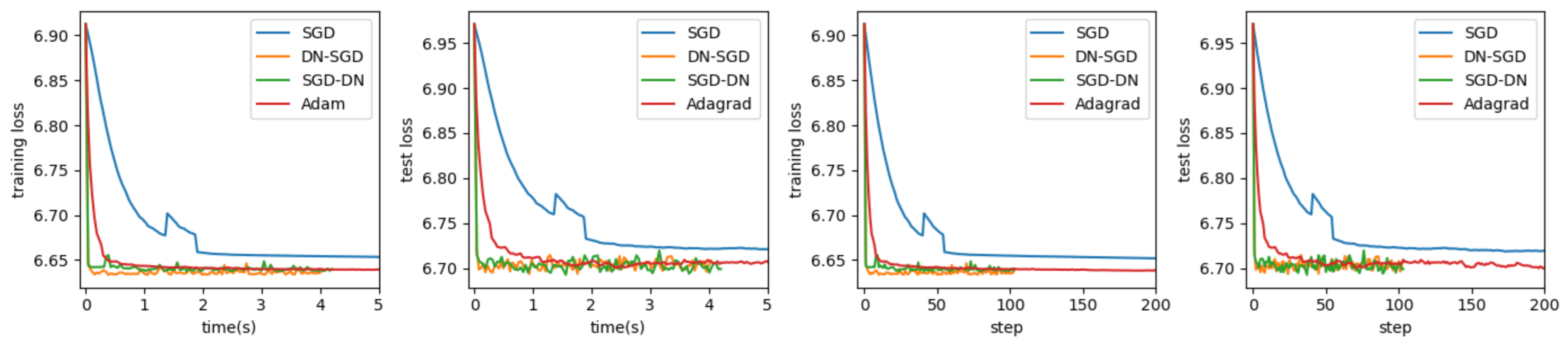
House Prices: The training set is of size 1361, and the test set is of size 100. A neural network with one hidden layer of size 5 and sigmoid activation function was used, i.e., $(n_0,n_1,n_2)=(288,5,1)$, where the first and last layers are the size of the input and output, respectively. The output layer has no activation function except with MSE, and the learning rate for SGD was set to be 0.01—the same as other methods for comparison purposes. Each algorithm was run for 20 epochs. The website is https://www.kaggle.com/c/house-prices-advanced-regression-techniques/data (accessed on 25 March 2021). The results are presented in Figure 1.

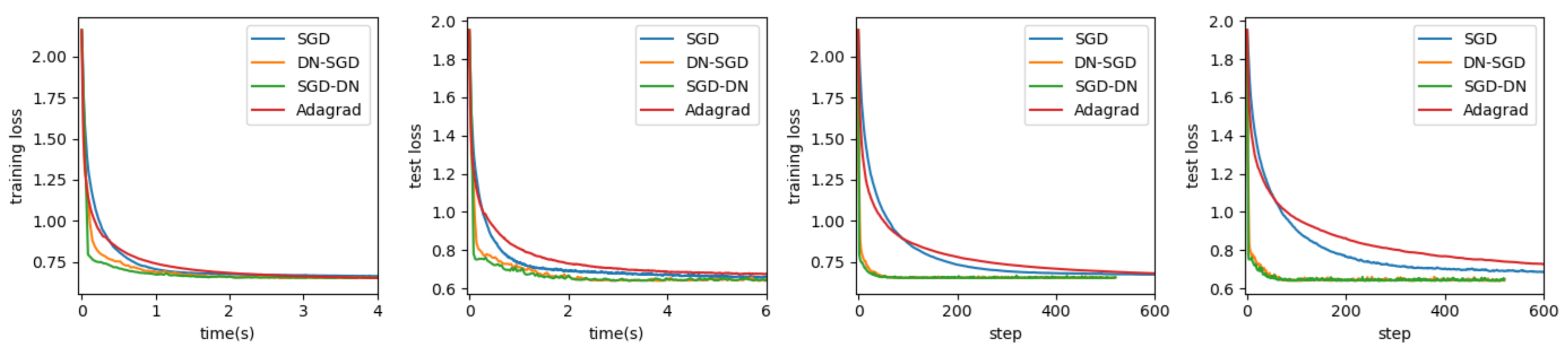
Housing Market: The training set is of size 20,473, and the test set is of size 10,000. A neural network with one hidden layer of size 4 and sigmoid activation function was used, i.e., $(n_0,n_1,n_2)=(451,4,1)$, where the first and last layers are the size of the input and output, respectively. The output layer has no activation function except with MSE, and the learning rate for SGD was set to be 0.001—the same as other methods for comparison purposes. Each algorithm was run for five epochs. The website is https://www.kaggle.com/c/sberbank-russian-housing-market/data (accessed on 25 March 2021). The results are presented in Figure 2.

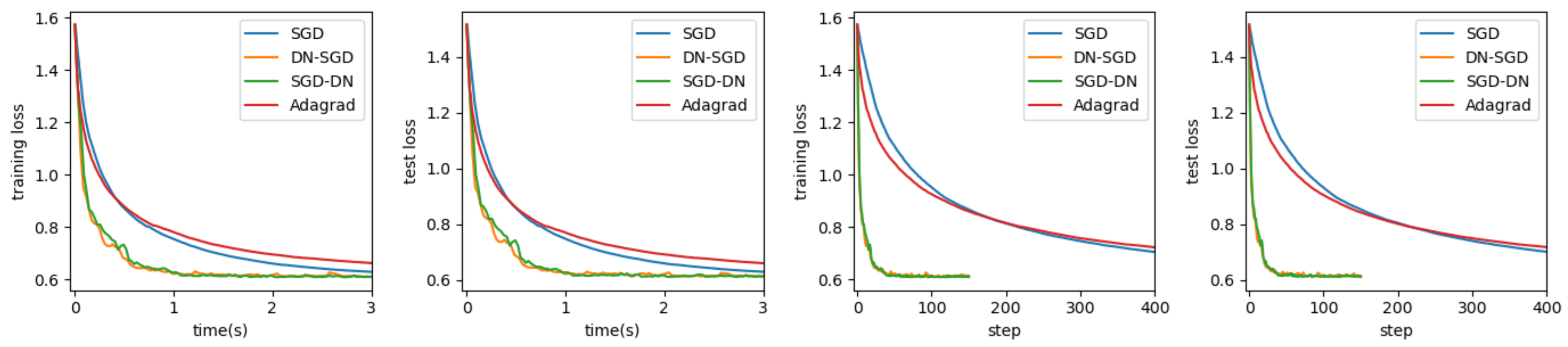
Cabbage Price: The training set is of size 2423, and the test set is of size 500. A neural network with one hidden layer of size 6 and sigmoid activation function was used, i.e., $(n_0,n_1,n_2)=(4,6,1)$, where the first and last layers are the size of the input and output, respectively. The output layer has no activation function except with MSE, and the learning rate for SGD was set to be 0.01—the same as other methods for comparison purposes. Each algorithm was run for five epochs. The website is https://www.kaggle.com/c/regression-cabbage-price/data (accessed on 25 March 2021). The results are presented in Figure 3.

5.2. Classification Problem

The performance of the algorithms DN-SGD and SGD-DN was compared with SGD Adagrad, the experiments were performed on several classification problems, and both training loss and testing loss are provided. The datasets were scaled to have normal distribution.

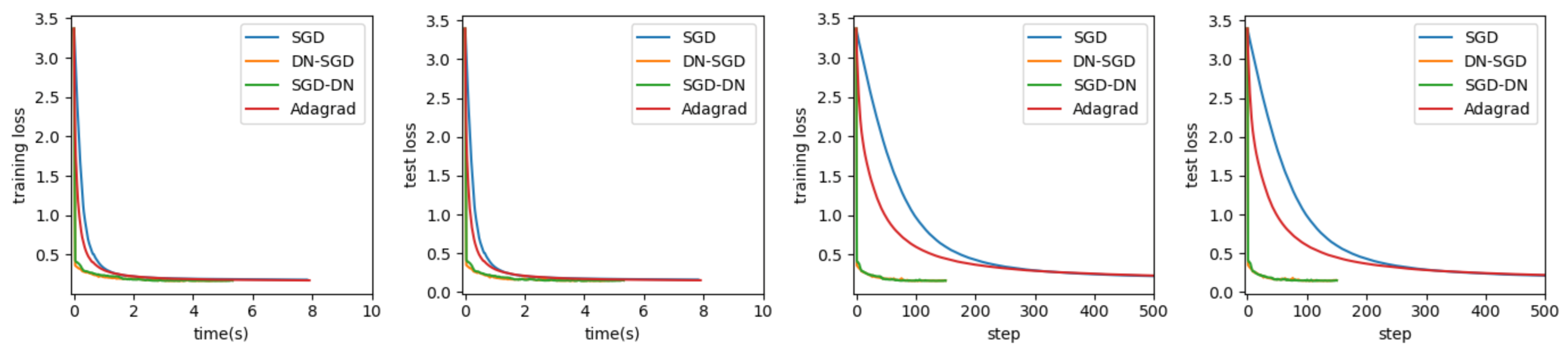
Shot Selection: The training set is of size 20,698, and the test set is of size 10,000. A neural network with one hidden layer of size 6 and sigmoid activation function was used, i.e., $(n_0,n_1,n_2)=(228,6,2)$, where the first and last layers are the size of the input and output, respectively. The output layer has softmax with cross entropy, and the learning rate for SGD was set to be 0.01—the same as other methods for comparison purposes. Each algorithm was run for 25 epochs. The website is https://www.kaggle.com/c/kobe-bryant-shot-selection/data (accessed on 25 March 2021). The results are presented in Figure 4.

Categorical Feature Encoding: The training set is of size 30,000, and the test set is of size 10,000. A neural network with one hidden layer of size 6 and sigmoid activation function was used, i.e., $(n_0,n_1,n_2)=(96,4,2)$, where the first and last layers are the size of the input and output, respectively. The output layer has softmax with cross entropy, and the learning rate for SGD was set to be 0.01—the same as other methods for comparison purposes. Each algorithm was run for 20 epochs. The website is https://www.kaggle.com/c/cat-in-the-dat/data (accessed on 25 March 2021). The results are presented in Figure 5.

Santander Customer Satisfaction: The training set is of size 30,000, and the test set is of size 10,000. A neural network with one hidden layer of size 4 and sigmoid activation function was used, i.e., $(n_0,n_1,n_2)=(369,4,2)$, where the first and last layers are the size of the input and output, respectively. The output layer has softmax with cross entropy, and the learning rate for SGD was set to be 0.01—the same as other methods for comparison purposes. Each algorithm was run for 20 epochs. The website is https://www.kaggle.com/c/santander-customer-satisfaction/data (accessed on 25 March 2021). The results are presented in Figure 6.

6. Discussion of Results

From the experimental results, it can be seen that DN-SGD and SGD-DN are always faster than SGD and Adagrad in terms of both steps and time, which is consistent with the provided analysis. In addition, when the dataset is huge, the DN-SGD and SGD-DN can be more efficient because the advantage of quick descent can exceed the cost of computing the second-order information. DN-SGD is to find the optimal point for the parameters of last layer and then update other parameters using SGD in each iteration. SGD-DN is to update parameters, except the last layer using SGD, and then find the optimal point for the parameters of the last layer in each iteration. They both make full use of the convergence and rate of convergence of convexity of the last layer. We will analyze the experimental results in detail below.

6.1. Regression Problem

We performed our experiments on three real datasets: House Price, Housing Market, and Cabbage Price. In every experiment, we maintained the same DNNs model and initialization parameters to train DNNs using SGD, Adagrad, DN-SGD and SGD-DN. In

Table 1. Running time, iteration steps and minimum loss for regression problem. The numbers in bold are the optimal values.

Algorithm		House Prices			Housing Market			Cabbage Price
		Time (s)	Steps	Loss	Time (s)	Steps	Loss	Time (s)	Steps	Loss
Training	SGD	0.15	49	4.91	3.09	104	6.66	0.12	32	3.11
	DN-SGD	0.06	5	4.69	0.15	5	6.63	0.05	5	3.10
	SGD-DN	0.15	22	4.81	0.73	39	6.64	0.048	5	3.10
	Adagrad	0.05	23	4.91	2.97	86	6.64	0.10	48	3.10
Test	SGD	0.12	51	4.86	3.91	147	6.72	0.14	46	3.30
	DN-SGD	0.05	5	4.62	0.17	6	6.70	0.04	7	3.28
	SGD-DN	0.15	23	4.78	0.96	42	6.70	0.10	25	3.21
	Adagrad	0.05	23	4.86	3.23	75	6.70	0.11	41	3.30

, we can see that DN-SGD and SGD-DN perform consistently and they both perform better than SGD and Adagrad in terms of time and steps in both training datasets and testing datasets. The training loss curves and test loss curves of different optimization algorithms for regression tasks are shown in Figure 1, Figure 2 and Figure 3. Our proposed methods converge much faster than SGD and Adagrad. We can see from Figure 1 that the loss of using our DN-SGD method quickly decreases to a minimum point in no more than ten steps in both training loss and test loss in all three datasets. In the dataset House Price, on the contrary, using SGD, the loss decays much slower than our method in terms of clock time and steps and the minimum point is higher than DN-SGD. At the same time, Adagrad takes about the same amount of time to arrive a higher minimum point than DN-SGD. SGD-DN takes more time but also has a lower minimum point than Adagrad. Thus, DN-SGD and SGD-DN have a better generalization than SGD and Adagrad. In the dataset Housing Market, DN-SGD is nearly 20 times faster in converging to the stationary point than SGD and Adagrad in terms of time and steps in both training loss and test loss. In the dataset Cabbage Price, DN-SGD and SGD-DN also perform better than SGD and Adagrad in almost half the time and one-sixth of the steps. All of this suggests that SGD-DN and DN-SGD have a better convergence than SGD and Adagrad.

6.2. Classification Problem

For the classification task, we also experimented on three real datasets: Shot Selection, Categorical Feature Encoding, and Santander Customer Satisfaction. In every experiment, we also maintained the same DNNs model and initialization parameters to train DNNs using SGD, Adagrad, DN-SGD and SGD-DN. Obviously, we can see from

Table 2. Running time, iteration steps and minimum loss for classification problem. The numbers in bold are the optimal values.

Algorithm		Shot Selection			Categorical Feature			Santander Customer
		Time (s)	Steps	Loss	Time (s)	Steps	Loss	Time (s)	Steps	Loss
Training	SGD	2.89	476	0.70	2.76	451	0.64	1.98	451	0.23
	DN-SGD	1.49	39	0.69	1.13	49	0.62	1.93	73	0.22
	SGD-DN	1.43	37	0.69	1.13	49	0.62	1.93	74	0.22
	Adagrad	3.11	531	0.70	2.73	432	0.67	1.95	446	0.23
Test	SGD	4.13	425	0.71	2.74	447	0.64	1.97	448	0.23
	DN-SGD	2.19	51	0.64	1.09	49	0.62	1.92	71	0.22
	SGD-DN	2.15	49	0.64	1.09	49	0.62	1.92	73	0.22
	Adagrad	4.27	437	0.73	2.71	425	0.67	1.94	439	0.23

that SGD-DN and DN-SGD perform better than SGD and Adagrad, however, the performance is worse than for regression task. This is because the Hessian matrix for the classification task has a bigger size than the regression task so computing the inverse matrix takes more time. In addition, we can see that DN-SGD and SGD-DN perform consistently in both time and steps. In the datasets Shot Selection and Categorical Feature Encoding, the loss of using our DN-SGD method quickly decreases to a minimum point in several steps. On the contrary, using SGD and Adagrad, the loss decays much slower than our method in terms of clock time and steps and the minimum point is higher than DN-SGD and SGD-DN. Thus, DN-SGD and SGD-DN have a better generalization than SGD and Adagrad. In the dataset Santander Customer Satisfaction, DN-SGD, SGD-DN, SGD and Adagrad take almost the same time to reach the same stationary point, however, DN-SGD and SGD-DN take less steps than SGD and Adagrad. Anyway, SGD-DN and DN-SGD perform better in convergence and generalization. In Table 2, what we have in bold is the optimal value.

7. Conclusions and Future Research Directions

In this paper, we propose the DN-SGD and SGD-DN methods combining the stochastic gradient descent and damped Newton method, which perform better than SGD and Adagrad in several datasets for training neural networks. These methods also have the potential for application on more sophisticated models such as CNNs, ResNet and even GNNs which are proposed on the basis of multilayer neural network (MLP). These complicated models can have convexity for the parameters of the last layer with a high probability, therefore we can make full use of the convexity to come up with the corresponding efficient algorithms. However, it is very hard to do this mathematically due to the complexity of computing the Hessian matrix in mathematical symbols and the great difficulty of using the naked eye to determine whether the Hessian matrix is positive definite or semi-positive definite. Nonetheless, we think it is a challenging and attracting topic in the area of deep learning optimization. Another promising future research topic is the study of the convexity of the Hessian matrix for each hidden layer, which is more difficult to do in rigorous mathematical methods.

References

- Gardner, W.A. Learning characteristics of stochastic-gradient-descent algorithms: A general study, analysis, and critique. Signal Process. 1984, 6, 113–133. [Google Scholar] [CrossRef]
- Qian, N. On the momentum term in gradient descent learning algorithms. Neural Netw. 1999, 12, 145–151. [Google Scholar] [CrossRef]
- Duchi, J.; Hazan, E.; Singer, Y. Adaptive subgradient methods for online learning and stochastic optimization. J. Mach. Learn. Res. 2011, 12, 2121–2159. [Google Scholar]
- Hardt, M.; Recht, B.; Singer, Y. Train faster, generalize better: Stability of stochastic gradient descent. In Proceedings of the 33rd International Conference on Machine Learning, New York, NY, USA, 19–24 June 2016; pp. 1225–1234. [Google Scholar]
- Liu, L.; Jiang, H.; He, P.; Chen, W.; Liu, X.; Gao, J.; Han, J. On the variance of the adaptive learning rate and beyond. arXiv 2019, arXiv:1908.03265. [Google Scholar]
- Ge, R.; Huang, F.; Jin, C.; Yuan, Y. Escaping from saddle points—Online stochastic gradient for tensor decomposition. In Proceedings of the 28th Conference on Learning Theory, Paris, France, 2–6 July 2015; pp. 797–842. [Google Scholar]
- Alain, G.; Roux, N.L.; Manzagol, P.A. Negative eigenvalues of the hessian in deep neural networks. arXiv 2019, arXiv:1902.02366. [Google Scholar]
- Grosse, R.; Martens, J. A kronecker-factored approximate fisher matrix for convolution layers. In Proceedings of the 33rd International Conference on Machine Learning, New York, NY, USA, 20–22 June 2016; pp. 573–582. [Google Scholar]
- Martens, J.; Grosse, R. Optimizing neural networks with kronecker-factored approximate curvature. In Proceedings of the 32nd International Conference on Machine Learning, Lille, France, 6–14 July 2015; pp. 2408–2417. [Google Scholar]
- Martens, J.; Ba, J.; Johnson, M. Kronecker-factored curvature approximations for recurrent neural networks. In Proceedings of the 6th International Conference on Learning Representations, Vancouver, BC, Canada, 30 April–3 May 2018; pp. 1–25. [Google Scholar]
- Martens, J. Deep learning via hessian-free optimization. In Proceedings of the 27th International Conference on International Conference on Machine Learning, Haifa, Israel, 21–24 June 2010; pp. 735–742. [Google Scholar]
- Xu, P.; Roosta, F.; Mahoney, M.W. Newton-type methods for non-convex optimization under inexact hessian information. Math. Program. 2020, 184, 35–70. [Google Scholar] [CrossRef] [Green Version]
- Kiros, R. Training neural networks with stochastic hessian-free optimization. arXiv 2013, arXiv:1301.3641. [Google Scholar]
- Martens, J.; Sutskever, I. Training deep and recurrent networks with hessian-free optimization. In Neural Networks: Tricks of the Trade; Springer: Berlin/Heidelberg, Germany, 2012; pp. 479–535. [Google Scholar]
- Botev, A.; Ritter, H.; Barber, D. Practical gauss-newton optimisation for deep learning. In Proceedings of the 2017 International Conference on Machine Learning, Sydney, Australia, 6–11 August 2017; pp. 557–565. [Google Scholar]
- George, T.; Laurent, C.; Bouthillier, X.; Ballas, N.; Vincent, P. Fast approximate natural gradient descent in a kronecker-factored eigenbasis. arXiv 2018, arXiv:1806.03884. [Google Scholar]
- Amari, S.i.; Park, H.; Fukumizu, K. Adaptive method of realizing natural gradient learning for multilayer perceptrons. Neural Comput. 2000, 12, 1399–1409. [Google Scholar] [CrossRef] [PubMed]
- Pascanu, R.; Bengio, Y. Revisiting natural gradient for deep networks. arXiv 2013, arXiv:1301.3584. [Google Scholar]
- Bottou, L.; Curtis, F.E.; Nocedal, J. Optimization methods for large-scale machine learning. Siam Rev. 2018, 60, 223–311. [Google Scholar] [CrossRef]
- Ren, Y.; Goldfarb, D. Efficient subsampled Gauss–Newton and natural gradient methods for training neural networks. arXiv 2019, arXiv:1906.02353. [Google Scholar]
- Cai, T.; Gao, R.; Hou, J.; Chen, S.; Wang, D.; He, D.; Zhang, Z.; Wang, L. A gram-gauss-newton method learning overparameterized deep neural networks for regression problems. arXiv 2019, arXiv:1905.11675. [Google Scholar]
- Goldfarb, D.; Ren, Y.; Bahamou, A. Practical quasi-Newton methods for training deep neural networks. arXiv 2020, arXiv:2006.08877. [Google Scholar]
- Ren, Y.; Goldfarb, D. Kronecker-factored Quasi–Newton Methods for Convolutional Neural Networks. arXiv 2021, arXiv:2102.06737. [Google Scholar]
- Byrd, R.H.; Hansen, S.L.; Nocedal, J.; Singer, Y. A stochastic quasi-Newton method for large-scale optimization. SIAM J. Optim. 2016, 26, 1008–1031. [Google Scholar] [CrossRef]
- Wang, X.; Ma, S.; Goldfarb, D.; Liu, W. Stochastic quasi-Newton methods for nonconvex stochastic optimization. SIAM J. Optim. 2017, 27, 927–956. [Google Scholar] [CrossRef] [Green Version]
- Goodfellow, I.; Bengio, Y.; Courville, A.; Bengio, Y. Deep Learning; MIT Press: Cambridge, MA, USA, 2016. [Google Scholar]
- Horn, R.A.; Johnson, C.R. Matrix Analysis; Cambridge University Press: Cambridge, UK, 2012. [Google Scholar]
- Steeb, W.H.; Shi, T.K. Matrix Calculus and Kronecker Product with Applications and C++ Programs; World Scientific: Singapore, 1997. [Google Scholar]
Figure 1.
Results on House Price regression problem with .
Figure 2.
Results on Housing Market regression problem with .
Figure 3.
Results on Cabbage Price regression problem with .
Figure 4.
Results on Shot Selection classification problem with .
Figure 5.
Results on Categorical Feature Encoding classification problem with .
Figure 6.
Results on Santander Customer Satisfaction classification problem with .